This document describes an experiment that analyzed when combining two visual cognition systems can lead to better performance than the individual systems. The experiment involved 20 trials where pairs of participants observed an object being thrown and independently guessed its landing location. The document discusses: 1) How the individual guesses and confidence levels were used to establish scoring systems and calculate statistical means for combining the systems. 2) The concept of cognitive diversity, which measures how distinct the scoring systems are from each other, and performance ratio, which compares the relative accuracy of the individual systems. 3) The results showed that on average, combining two visual cognition systems leads to better performance than the individual systems only if the systems have high performance ratio and cognitive diversity.

1. When to Combine Two Visual Cognition Systems?
Darius A. Mulia1, Charles R. Skelsey1, Lihan Yao1, Dougan J. McGrath1, and D. Frank Hsu2
Laboratory of Informatics and Data Mining
Department of Computer and Information Science
Fordham University
New York, NY 10023
Email:
{dmulia,cskelsey,lyao1, dmcgrath}@fordham.edu1
hsu@cis.fordham.edu2
Abstract—In computing, informatics and other scientific disci-
plines, combinations of two or more systems have been shown to
perform better than individual systems. Although combinations
of multiple systems can be better than each individual system,
it is not known when and how this is the case. In this paper,
we focus on visual cognition systems. In particular, we conduct
an experiment consisting of twenty trials, each focused on a pair
of visual cognition systems. The data set is then analyzed using
combinatorial fusion. Our results demonstrate that on average,
combination of two visual cognition systems can perform better
than individual systems only if the individual systems have high
performance ratio and cognitive diversity. These results provide
a necessary condition as to when two cognition systems should
be combined to achieve better outcomes. These results provide a
necessary condition as to when two cognition systems should be
combined to achieve better outcomes.
I. INTRODUCTION
Research in decision-making carries wide-reaching applica-
tions such as visual screening, image analysis, task allocation,
etc. Recent work by Bahrami [1] has focused on studying
how decisions made by pairs of individuals can contribute to
a better performing joint decision in perceptual and visually-
oriented tasks. Ernst et al. [5] expanded Bahrami’s study
into a hypothetical example. Two referees freely exchange
information to aid in their decision of whether the ball crosses
the goal line. More recently, Koriat [9] stipulated that choosing
the more confident participant in a pair, without information
exchange between the two individuals, could outperform either
participant. While Koriat analyzes joint decisions between
non-communicating participants, Batallones et al. [2], [3],
McMunn-Coffran [13], [14], and Paolercio et al. [11] expand
the works of Bahrami and Ernst by further optimizing joint
visual cognition decisions.
Combinatorial fusion, a new information fusion paradigm,
was proposed and studied by Hsu et al [6]–[8]. It has been
successfully applied to domains such as feature selection and
combination [4], [10], skeleton pruning, target tracking [11],
[12], ChIP sequence peak detection [18], and virtual screening
[19]. Combinatorial fusion entails the combination of multiple
scoring systems. Cognitive diversity between two scoring
systems is used to decide when and how to combine these
systems. Other fusions have also been studied and discussed
[15], [16].
In this paper, we conduct an experiment of twenty trials.
Subjects observe a small object being thrown in a fashion
similar to previous experiments [2], [3], [13], [14], [17], where
they are separately asked of the object’s perceived landing
point. These subjects are treated as two visual cognition
systems in the physical space, and are connected to two scoring
systems in the common visual space. Both score combination
and rank combination are used to improve the combined
system. The concept of cognitive diversity is used to determine
when to combine and how to combine multiple systems.
Section II gives a framework for the combination if vi-
sual cognition systems. Section III describes the concept of
cognition diversity and performance ratios, both are used to
distinguish positive cases from negative cases in section V.
Section IV focus on our experiment results and remarks.
Section V describes the problem of when is the combination
of p and q better than each individual p and q using cognitive
diversity and performance ratio. In particular, the relation
between cognitive diversity and performance is explored using
two examples. Section VI concludes the paper with suggestion
for further work.
II. COMBINING TWO COGNITION SYSTEMS
A. Computing Statistical Means
Within the pair of participants, each individual, when tasked
with determining the location of an object, independently con-
siders a region of possible choices before making their deci-
sion and its corresponding confidence value. The decisions are
P,Q, representing the individual’s decision regarding where
the object A landed. The confidence factors of the individuals
is recorded as [σ = 0.5*r]. Here, r represents the radius of
the circle centered about each participants guess location of
A. [ maybe say that the larger the circle the less confident
and vice versa]. These confidence factors are emphasized to
varying degrees in the generation of the statistical means M0,
M1, and M2, calculated by:
Mi =
P
σi
P
+ Q
σi
Q
1
σi
P
+ 1
σi
Q
i = 0, 1, 2, (1)
where P, Q are the individual decisions, and σP , σQ are the
respective confidence values of P and Q.

2. P QP QM0
P QP QM1
P QP QM2
Fig. 1. Visualization of the CVS for M0, M1, and M2. Here, the line P Q
displays how the values i = 0, 1, 2 can affect the position of the statistical
mean Mi in relation to P and Q.
Each trial contains three calculations of a statistical means,
M0, M1 and M2. As the index of i increases, the weight of
the confidence factor values increases for each participants
decision. This increase of weight will exhibit a greater effect
on determining the statistical mean.
B. Constructing Common Visual Space
Each participant is treated as a visual cognition system
and their decisions were recorded as x- and y-coordinates.
This generated a Cartesian plane with points (Px,Py) and
(Qx,Qy). To evaluate this system, a line segment PQ is created
with points(Px,Py) and (Qx,Qy). To ensure that all of the
confidence factors σP , σQ, are counted, the line segment PQ
needs to be extended. The common visual space is constructed
from an extension of the line segment PQ where the larger
value PM (or QM) is extended by 50PM (or 1.5QM). MQ
is also extended to Q so that Mi is the midpoint of P Q .
The line segment P Q is divided into 63 intervals with
d1, d2, . . . , d63 as their midpoints. Since location P and Q are
two points in the common visual space P Q , we will construct
two scoring systems p and q based on P and Q respectively.
C. Establishing Scoring System
The line segment P Q is divided into 63 intervals with
d1, d2, . . . , d63 as their midpoints. Since location P and Q
are two points in the common visual space P Q , we will
construct two scoring systems p and q based on P and Q
respectively. It is assumed that each participant assigns the
highest score to the location where they think the object A
landed. Therefore, as we move away from this point, the score
decreases at a rate based on the participant?s confidence factor.
A higher score means a higher probability that their guess
is where A actually landed. A lower score indicates a lower
probability that their guess is where A landed. Each of the two
scoring systems p and q is then assigned a score to each of
the midpoints di, i = 1, 2, . . . , 63, according to the following
probability model by normal distribution based on P and Q
respectively.
f(x, µ, σ) =
1
σ
√
2π
e−
(x−µ)2
2σ2
(2)
Where x is a normal random variable, µ is the perceived
location of P (or Q), σ is the confidence radius of P (or
Q).
Each system p (or q) has a score function sp (or sq) on
D = {d1, d2, , d63}. Ranking di highest to lowest. The highest
rank will receive the lowest number, while the lower rank will
have a higher number. This creates our rank functions rP (or
rQ).
D. Rank and Score Combination
Once all the scores and ranks are calculated, the score
combination C, and the rank combination D, are calculated.
This function is defined as the following:
sC(dj) =
sp(dj) + sq(dj)
2
, j ∈ [1, 63] (3)
Where sp(dj) (or sq(dj) is the score function of p (or q). The
rank function D is defined as:
sD(dj) =
rp(dj) + rq(dj)
2
, j ∈ [1, 63] (4)
where rp(dj) (or rq(dj)) is the rank function.
The rank and score combinations produce points C(x,y)
and D(x,y) that are obtained from choosing the di in the
score combination and rank combination respectively with
rank one. These points will be used to calculate the distance
between C and A (actual) and also D and A (actual). These
distances between points are used to calculate the performance
of each location. Therefore, the performance of P, Q, M, D,
and C can be calculated and used to measure the accuracy of
combinatorial fusion.
III. COGNITIVE DIVERSITY AND PERFORMANCE RATIO
A. Computing Cognitive Diversity
Let sA and rA be the score function and rank function of the
scoring system A respectively. The Rank-Score Characteristic
(RSC) Function is defined as:
fA(i) = sA ◦ r−1
A (i) = sA r−1
A (i) (5)
where sA and rA are the score function and rank function of
the system A respectively [6]–[8]. The calculation of fA can
also be viewed as a transformation from the domain D for the
score function sA to the domain N for the RSC function [7],
[8].
The rank-score characteristics function can be computed by
sorting the score values in sA(dj), where j ∈ [1, 63], using
the rank values as the key. The cognitive diversity between
systems p and q, d(p, q), defined by the two RSC functions
fp, fq of the scoring systems p and q measures how distinct
each scoring systems relative to other scoring systems. We
calculate d(p, q) = d(fp, fq) by:
d(p, q) =
63
i=1
(fp(i) − fq(i))2
63
(6)
Hsu and Taksa [6] showed that under certain condition
including high cognitive diversity, rank combination is better
than score combination results.

3. B. Calculating Performance Ratio
The relative performance of individual systems within a trial
is called the Performance Ratio. Let A and B be two scoring
systems with performance P(A) and P(B) respectively. Let
Pl and Ph be the minimum (and maximum) of {P(A), P(B)}
respectively. The ratio Pl/Ph is then normalized to (0, 1].
C. Positive vs. Negative Cases
As in formula (3) and (4), if performance of C, PC (or
performance of D, PD) is better than or equal to the best
of PA and PB, the combination C (or D) is a positive case.
Otherwise, the combination is of a negative case. We will plot
positive cases and negative cases against performance ratio as
the x- axis and diversity as the y- axis in Section V .
IV. EXPERIMENT
A. Data Collection
For experimental data acquisition, a 300 by 360 inch grid
is constructed in a public park. 20 pairs of participants were
randomly selected from individuals in the park, with pairs of
2 participants constituting each experimental set. Each pair is
led to a line 40 feet back from the marked grid, where they are
instructed to observe a coordinator throwing a 1.5 by 1.5 inch
circular object into the grid. The coordinator is standing 40 feet
back from the grid, situated directly between the participants.
The object is constructed of metal washers connected together
in an irregular manner to minimize movement upon reaching
the ground, while being large enough to be visible while
airborne. This landscape and test environment is modeled on
the one used in [2], [3], [13], [14], [17], but with enhanced
visual clarity for the participant. The rectangular grid is
marked by yellow flags so that observers can clearly see the
boundary of the region.
After the object is thrown, each participant is asked to
independently direct two researchers, who are positioned at the
farthest opposite ends of the grid, to the location they believe
the object has landed. To avoid a bias occurring by having
one guess influence another, each of the two participants
moves a researcher simultaneously and independently. Once
both decisions are made, a token is placed at the point
chosen by each participant. The participants are then asked to
determine the confidence of their guess, with researchers using
an apparatus to aid the participants visually. Less confidence
would produce a wider radius, while more confidence would
result in a smaller radius, centered on their respective token
locations. These radii are projected visually onto the grid with
the aid of the apparatus, as to assist the participants with
making an appropriate confidence determination.
Once the confidence radii were recorded, the participants
were shown their token locations on the grid and dismissed.
The x- and y- coordinates for P, Q, and A are recorded
respectively by using distances determined from the edges of
the grid. Table I lists the 20 trials, coordinates of P, Q, and A,
and confidence radii for P and Q. This data set is labeled as
#111613.
TABLE I
EXPERIMENTAL DATA FROM DATA SET #111613
Trial (Px,Py) σP (Qx,Qy) σQ (Ax,Ay)
1 (95,326) 12 (90,406) 14 (93,413)
2 (267,346) 12 (270,323) 8 (258,331)
3 (156,279) 12 (157,279) 6 (166,283)
4 (175,185.5) 8 (157,177) 6 (161,180)
5 (200.5,304) 16 (206,357) 18 (203,344)
6 (101.5,258) 10 (92.5,288) 8 (108,288)
7 (232,288) 10 (238,298.5) 15 (253,297)
8 (25,92) 14 (35,394.5) 22 (10,427)
9 (215.5,165) 12 (172,187) 8 (159.5,222)
10 (106,120) 14 (83,152) 10 (88,154.5)
11 (279,158) 6 (272,160) 14 (284,163)
12 (128,148) 9 (137.5,221) 8 (137.5,227)
13 (233,256) 12 (248.5,201.5) 12 (233,256)
14 (214.5,363) 14 (221,360) 17 (227,266)
15 (148.5,154.5) 14 (90,120) 12 (112,145)
16 (49,128) 11 (88.5,133) 10 (62.5,153)
17 (190,124) 6 (172,154) 16 (190,125)
18 (257,257) 8 (246,258) 14 (245,251)
19 (96,270) 8 (83.5,231) 12 (99,231.5)
20 (95.5,255) 20 (77,271) 20 (79,270)
B. Combination of Scoring Systems p and q
After the data was obtained, the decision of Participant P,
marked as P, and the decision of Participant Q, marked as Q,
are used to obtain line segment PQ. We located the weighted
confidence mean of M0, M1, and M2 by using the confidence
radii of P and Q as the two sigma values, as in Section(II)(A).
Then we extended the line segment to P Q . In order to
join the two visual cognition systems, we need to establish
a common visual space that account for the visual space of
both participants. The 63 intervals along the P Q line serve
as the common visual space to be scored (see Section(II)(B).
When PQ has been divided into the 63 intervals based on
each of Mi, i = 0, 1, 2, the intervals are scored according to
the normal distribution of P and Q by using the location of P
and Q as the mean and σP and σQ as the standard deviation
respectively (see Section(II)(C)). Both systems assume the
set of common interval midpoints [d1, . . . , d63]. The score
functions sp(dj) and sq(dj) map each interval, dj to a score
in systems p and q respectively. The rank function rp(dj)
and rq(dj) map each dj to a positive integer j ∈ [1, 63] by
assigning 1 to the highest score and 63 to the lowest score to
each of the intervals dj.
For each of the three M0, M1, M2 analysis, we apply the
score combination C and rank combination D given by formula
(3) and (4). The highest score combination in the interval is
chosen as C and the lowest rank combination is chosen as D.
Then, we calculated the performance of each points P, Q, Mi,
C, D, for i = 0, 1, and 2 by calculating the distance of these
five points to the actual landing site A. The performances of
each point are ranked from 1 to 5. The point with the shortest
distance from the target is ranked 1 (see Figure.2).

4. Summary Result for Dataset #111613
M0 M1 M2 P Q M0 C D P Q M1 C D P Q M2 C D
Trial 1 (87,7.6) (12,14) 1 2 3 3 1 2 3 3 3 1 2 3 3 5 1 3 1 4
Trial 2 (17.5,14.4) (12,8) 2 1 3 4 2 1 2 4 5 3 1 3 2 5 4 1 2 2
Trial 3 (10.8,9.8) (12,6) 3 2 1 4 1 3 1 4 5 1 4 2 2 5 1 4 2 2
Trial 4 (15,5) (8,6) 3 2 1 4 1 3 1 4 4 3 1 4 2 4 3 1 4 2
Trial 5 (40.1,13.3) (16,18) 1 2 3 3 1 2 3 3 4 1 3 1 5 4 1 3 1 5
Trial 6 (30.7,15.5) (10,8) 3 2 1 4 1 3 1 4 4 2 3 4 1 4 2 3 4 1
Trial 7 (22.8,15.1) (10,15) 1 2 3 3 1 2 3 3 3 1 2 3 3 5 1 2 3 3
Trial 8 (38.1,41) (14,22) 3 2 1 1 5 4 1 1 1 5 4 2 2 2 5 4 3 1
Trial 9 (79.9,37.2) (12,8) 3 2 1 4 1 3 1 4 5 1 4 1 1 4 1 3 4 2
Trial 10 (38.9,5.6) (14,10) 3 2 1 4 1 3 1 4 5 2 4 2 1 4 2 3 4 1
Trial 11 (7.1,12.4) (6,14) 3 2 1 1 5 4 1 1 1 5 4 1 1 3 5 4 1 1
Trial 12 (79.6,6) (9,8) 3 2 1 3 1 2 3 3 4 1 3 4 2 4 1 3 4 2
Trial 13 (0,56.7) (12,12) 2 1 2 1 5 4 2 2 1 4 3 4 2 1 5 4 2 2
Trial 14 (97.8,94.2) (14,17) 1 2 3 3 1 2 3 3 5 1 2 3 3 5 1 2 3 3
Trial 15 (37.7,33.3) (14,12) 2 1 3 4 2 1 2 4 5 2 1 2 2 4 3 1 4 2
Trial 16 (28.4,32.8) (11,10) 1 2 3 2 4 1 4 2 2 5 1 2 4 2 5 1 2 4
Trial 17 (1,34.1) (6,16) 3 2 1 3 5 4 1 1 1 5 4 2 2 1 5 4 2 2
Trial 18 (13.4,7.1) (8,14) 1 2 3 3 1 2 3 3 3 1 2 3 3 3 1 2 4 4
Trial 19 (38.6,15.5) (8,12) 1 2 3 3 1 2 3 3 3 1 2 3 3 5 1 3 1 4
Trial 20 (22.3,2.2) (20,20) 2 3 1 3 1 2 3 3 4 1 3 1 4 3 1 2 3 3
Combination Results from Data set #111613 with 20 trials
Trial (a): Per (P,Q) (b): Conf.Rad(P,Q)
(c): Rank (d):Rank(P,Q,Mi,C,D) for i= 0,1, 2
Fig. 2. Results from Data Set #111613 with 20 trials
C. Results and Remarks
The first column labeled Trial is the specific trial that was
analyzed. Column (a) provides the performances of P and Q
in inches, which is the distance between P and the actual A,
and the distance between Q and actual A.
Column (b) provides the confidence radii of P and Q. In
(b), there are green, white, and gray cells. The green cells
indicate that choosing the more confident system would lead
to the more optimal decision (by Koriats criteria). The gray
cells indicate that confidence radii are equal, implying that
Koriats criteria does not apply. The white cells indicate that
choosing the more confident system (P or Q) does not lead to
an optimal decision.
In column (c), we rank the relative performance of weighted
means M0, M1, and M2 against one another, within the scope
of each trial. A yellow cell indicates that the weighted mean
is the highest ranked performer among P, Q, Mi, C, and D.
White cells indicate that the weighted mean is not the highest
ranked performer among its respective values of P, Q, Mi, C,
and D.
Column (d) is divided up into 3 sub-columns. Each sub-
column ranks P, Q, Mi, C, and D in descending order of
performance for i = 0, 1, and 2. The number 1 indicates
the best (or closest) performance to actual A, while the
number 5 indicates the worst (or farthest) performance from
A. Multiple occurring values imply that a tie has occurred
for a performance ranking. If, for example, both C and D
have the same interval di’s their optimal decision, then they
will share the same performance. Subsequently, they share the
same performance rank. Red cells indicate when the score
combinations (D) (or the rank combination (C)) are superior
to the individual performances of P and Q. Gray cells indicate
when C (or D) shares the same performance as the best
performer of P and Q. White cells (in the columns of C and
D) indicate when C (or D) fails to provide a superior decision
when compared to P and Q.
Our results demonstrate that CFA is a viable method to
combine two visual cognition systems. 15 out of 20 total trials
perform better than or equal to the best performer of P or
Q. This gives an improvement rate of approximately 75%.
Koriat’s Criterion only gives 65% correct rate (13 out of 20
trials). The only case not covered by Koriat?s criterion or by
the CFA framework is Trial 7, 14, and 18. Trial 1, 5, 16,
and 19, which cannot be covered by Koriat?s criterion can be
improved by CFA method, while Trial 12, on which CFA does
not perform well, can be covered by Koriat?s criterion.
Overall, CFA method compares favorably to the statistical
mean Mi, i = 0,1,2. M0 improves P,Q in 3 out of 20 trials,
while CFA improves M0 in 14 out of 20 trials. M1 improves
P,Q in 4 out of 20 trials, while CFA improves M1 in 14 out of
20 trials. Finally, M2 improves P,Q in 4 out of 20 trials, while
CFA improves M2 in 13 out of 20 trials. This demonstrates
that the CFA framework compares favorably with the statistical
means Mi, i = 0,1,2.

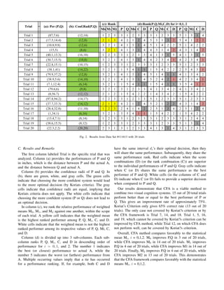
5. In M0 and M1, combination systems perform at least as well
as the better individual system of the trial, denoted by grey
cells in column (b) of Figure.2, Combination improvements
become more drastic with higher confidence emphasis. CFA
only improves Trial 17 in M0, and Trial 2, 4, 6, 10 in M1.
When the confidence is weighted more, CFA improves Trial
8, 11, and 15 in addition to improved trial in M1. With
increasing variance, the frequency of strictly positive cases
(where combination systems outperform individual systems)
increases, denoted by red cells.
In the comparison between rank combinations and score
combinations across statistical means, there is a direct rela-
tionship between variance and the amount of positive cases
for rank, i.e. four positive cases M0, seven positive cases for
first power variance M1, and seven positive cases for second
power variance M2. In contrast, the amount of positive cases
for score combinations diminish with increasing variance, i.e.
ten positive cases for no variance M0, eight positive cases for
first power variance, and six positive cases for second power
variance M2. This signifies, when performing combinatorial
fusion, that score combination is preferred without knowledge
of confidence measurements. Rank combination is preferred
with accurate knowledge of the confidence measurement.
Although M0 shows more successes than other WCS of
i = 1,2, but most of the outcomes are similar to the in-
dividual systems. This is clearly shown in ten trials where
the score combination and rank combination is in majority
just a duplicate of the individual systems. However, when we
take into account the individuals confidences, there are slight
improvement with the outcome in which the combinations
actually improve the individual performances. Note that only
system D that improve overall individual performances by
four trials while score combination remains not improving
individual systems. When we intensify the confidences even
more, the performance of both C and D improve more trials.
Score combination improves two trials while rank combination
improves all seven trials that show improvement. Overall, rank
combination seems to perform better than score combination.
V. WHEN IS COMBINATION OF P AND Q BETTER?
As mentioned in Paolercio et al. [17], the fusion of two
visual cognition systems can be better than each of the
individual when the two systems perform relatively good and
they are cognitively diverse. In our result, we test this argument
by plotting the performance ratio of the individual systems vs.
the cognitive diversity in Figure.3.
Figure.3 depicts positive cases and negative cases with
respect to criteria, i.e. Cognitive Diversity vs. performance
ratio calculated in Section III. Circle ”o” is the center of all
positive cases where combinations of P and Q are better or
equal to the best of P and Q. ”x” denotes the center of all
negative cases where the combined system of P and Q are
but a positive case. Overall, we see that Cognitive Diversity
and performance ratio can be used to discriminate positive vs.
negative cases. v
Performance Ratio(plow/phigh)
0.3 0.4 0.5 0.6 0.7 0.8
Cognitive Diversity d(P, Q)
0.2
0.3
0.4
0.5
0.6
0.7
0.8
x
x
x
M0
M1
M2
Positive Cases
Negative Cases
Fig. 3. Positive and Negative Cases on Cognitive Diversity vs Performance
Ratio
Figure.3 presents the positive cases having higher perfor-
mance ratio and cognitive diversity than the negative cases
overall. This is shown in M0 in which the positive case has
performance ratio and cognitive diversity of approximately 0.5
while the negative case has performance ratio of approximately
0.28 and cognitive diversity of approximately 0.22. In M1 and
M2, the cognitive diversity is lower than the cognitive diversity
in M1 but it is still relatively higher than the negative case of
the respective Mi values. The same understanding also applies
to the performance ratio of the individual systems. Overall, the
fusion of two visual perception systems is positive if the pair
has a higher performance ratio and cognitive diversity.
For all trials, by averaging cognitive diversity values and
relative performance ratios according to statistical means,
Figure 3 verifies the conditions for positive cases posed in
Yang et. al. [19].
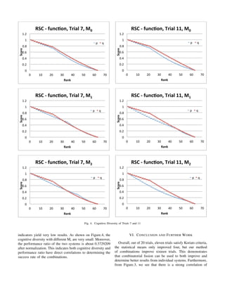
Figure. 4 gives cognition diversity of Trials 7 and 11
based on Mi, i = 0,1,2. In trial 11, combination performance
gives satisfactory outcome and the more we emphasize the
confidence of the individuals, the better the result. When
weighted sharing mean with i = 0, combination agrees on the
best of the two individual systems. As we put more weight
on the confidence, combination produces a better result than
each individual systems. This result falls according to our
assumption that if there is a high cognitive diversity and higher
performance ratio, combination can work better. Trial 11 has a
high cognitive diversity, where we observe cognitive diversity
increasing as shown in Figure 4 as we add more consideration
to the confidence. Trial 11 also has a high performance ratio of
1 after normalized, which means that trial 11 has the highest
performance ratio than all the other trials.
On the contrary, we can see the opposite in trial 7 in
which combination does not improve any of the individual
systems. We can argue that the failure of combinations is due
to the system with higher confidence performs poorly than
the other system. However, when we dissect more closely
on the cognitive diversity and the relative performance, both

6. 1"
"
"
!
"
"
"
"
"
"
!
"
"
"
"
"
0"
0.2"
0.4"
0.6"
0.8"
1"
1.2"
0" 10" 20" 30" 40" 50" 60" 70"
Score!
Rank!
RSC!,!func/on,!Trial!7,!M0!
p" q"
0"
0.2"
0.4"
0.6"
0.8"
1"
1.2"
0" 10" 20" 30" 40" 50" 60" 70"
Score!
Rank!
RSC!,!func/on,!Trial!7,!M1!
p" q"
0"
0.2"
0.4"
0.6"
0.8"
1"
1.2"
0" 10" 20" 30" 40" 50" 60" 70"
Score!
Rank!
RSC!,!func/on,!Trial!7,!M2!
p" q"
0"
0.2"
0.4"
0.6"
0.8"
1"
1.2"
0" 10" 20" 30" 40" 50" 60" 70"
Score!
Rank!
RSC!,!func/on,!Trial!11,!M0!
p" q"
0"
0.2"
0.4"
0.6"
0.8"
1"
1.2"
0" 10" 20" 30" 40" 50" 60" 70"
Score!
Rank!
RSC!,!func/on,!Trial!11,!M1!
p q"
0"
0.2"
0.4"
0.6"
0.8"
1"
1.2"
0" 10" 20" 30" 40" 50" 60" 70"
Score!
Rank!
RSC!,!func/on,!Trial!11,!M2!
p" q"
Fig. 4. Cognitive Diversity of Trials 7 and 11
indicators yield very low results. As shown on Figure.4, the
cognitive diversity with different Mi are very small. Moreover,
the performance ratio of the two systems is about 0.3729209
after normalization. This indicates both cognitive diversity and
performance ratio have direct correlations to determining the
success rate of the combinations.
VI. CONCLUSION AND FURTHER WORK
Overall, out of 20 trials, eleven trials satisfy Koriats criteria,
the statistical means only improved four, but our method
of combinations improve sixteen trials. This demonstrates
that combinatorial fusion can be used to both improve and
determine better results from individual systems. Furthermore,
from Figure.3, we see that there is a strong correlation of

7. cognitive diversity and performance ratio with the success rate
of combinatorial fusion.
Although our results apply to combination of visual cogni-
tion systems, it can be also applied to joint decision making
between two decision systems. In addition, the result can be
applied to the scenario where two sensors S1 and S2 are used
to detect the target T (which can be toxic waste or a destructive
object). The aim is to combine the evidence or findings from
S1 and S2 in order to improve the detection accuracy rate.
For further study, we will continue to add more trials to
the data pool and use the combination algorithm to analyze
different aspects of the data and how it affects decision
making, like gender or occupation. We look to conduct trials
where more people are added to each experiment as well. Our
research has demonstrated that combinatorial fusion can serve
as a useful tool in understanding and analyzing how to derive
the best decision from a pair of individually made decisions,
including visual cognition systems.
REFERENCES
[1] Bahrami, B., Olsen, K., Latham, P. E., Roepstorff, A., Rees, G., & Frith,
C. D. (2010). Optimally interacting minds. Science, 329(5995), 1081-
1085.
[2] Batallones, A., McMunn-Coffran, C., Sanchez, K., Mott, B., & Hsu,
D. F. (2012). Comparative study of joint decision-making on two
visual cognition systems using combinatorial fusion. In Active Media
Technology (pp. 215-225). Springer Berlin Heidelberg.
[3] Batallones, A., Sanchez, K., Mott, B., McMunn-Coffran, C., & Hsu, D.
F. (2013). Combining Two Visual Cognition Systems Using Confidence
Radius and Combinatorial Fu-sion. In Brain and Health Informatics (pp.
72-81). Springer International Publishing.
[4] Deng, Y., Wu, Z., Chu, C. H., Zhang, Q., & Hsu, D. F. (2013).
Sensor Feature Selection and Combination for Stress Identification
Using Combinatorial Fusion.International Journal of Advanced Robotic
Systems, 10, 1-10.
[5] Ernst, M. O. (2010). Decisions made better. Science(Washington),
329(5995), 1022-1023.
[6] Hsu, D. F., & Taksa, I. (2005). Comparing rank and score combination
methods for data fusion in information retrieval. Information Retrieval,
8(3), 449-480.
[7] Hsu, D. F., Chung, Y. S., & Kristal, B. S. (2006). Combinatorial fusion
analysis: methods and practice of combining multiple scoring systems.
Advanced Data Mining Technologies in Bioinformatics, 1157-1181.
[8] Hsu, D. F., Kristal, B. S., & Schweikert, C. (2010). Rank-score char-
acteristics (RSC) function and cognitive diversity. In Brain Informatics
(pp. 42-54). Springer Berlin Heidelberg.
[9] Koriat, A. (2012). When Are Two Heads Better than One and Why?.
Science,336(6079), 360-362.
[10] Lin, K. L., Lin, C. Y., Huang, C. D., Chang, H. M., Yang, C. Y., Lin,
C. T., & Hsu, D. F. (2007). Feature selection and combination criteria
for improving accuracy in protein structure prediction. NanoBioscience,
IEEE Transactions on, 6(2), 186-196.
[11] Liu, H., Wu, Z. H., Zhang, X., & Frank Hsu, D. (2013). A skeleton
pruning algorithm based on information fusion. Pattern Recognition
Letters.1138-1145.
[12] Lyons, D. M., & Hsu, D. F. (2009). Combining multiple scoring systems
for target track-ing using rankscore characteristics. Information Fusion,
10(2), 124-136.
[13] McMunn-Coffran, C., Paolercio, E., Liu, H., Tsai, R., & Hsu, D.
F. (2011, August). Joint decision making in visual cognition using
Combinatorial Fusion Analysis. In Cognitive Informatics & Cognitive
Computing (ICCI* CC), 2011 10th IEEE International Conference on
(pp. 254-261). IEEE.
[14] McMunn-Coffran, C., Paolercio, E., Fei, Y., & Hsu, D. F. (2012,
August). Combining multiple visual cognition systems for joint decision-
making using combinatorial fusion. In Cognitive Informatics & Cogni-
tive Computing (ICCI* CC), 2012 IEEE 11th International Conference
on (pp. 313-322). IEEE.
[15] Mohammed, S., & Ringseis, E. (2001). Cognitive diversity and consen-
sus in group deci-sion making: The role of inputs, processes, and out-
comes.Organizational Behavior and Human Decision Processes, 85(2),
310-335.
[16] Ng, K. B., & Kantor, P. B. (2000). Predicting the effectiveness of
naive data fusion on the basis of system characteristics. Journal of the
American Society for Information Sci-ence, 51(13), 1177-1189.
[17] Paolercio, E., McMunn-Coffran, C., Mott, B., Hsu, D. F., & Schweikert,
C. (2013, July). Fusion of two visual perception systems utilizing
cognitive diversity. In Cognitive Informatics & Cognitive Computing
(ICCI* CC), 2013 12th IEEE International Conference on (pp. 226-235).
IEEE.
[18] Schweikert, C., Brown, S., Tang, Z., Smith, P. R., & Hsu, D. F.
(2012). Combining multiple ChIP-seq peak detection systems using
combinatorial fusion. BMC genomics, 13(Suppl 8), S12.
[19] Yang, J. M., Chen, Y. F., Shen, T. W., Kristal, B. S., & Hsu, D. F.
(2005). Consensus scoring criteria for improving enrichment in virtual
screening. Journal of Chemical Information and Modeling, 45(4), 1134-
1146.