MRQAP	
tutorial	
Fariba	Karimi	
Fariba.karimi@gesis.org	
24.11.2015
Mul=ple	Regression	Quadra=c	
Assignment	Procedure
Why	regression	in	network	analysis?	
•  Inferen=al	sta=s=cs	have	proven	to	have	very	
useful	applica=ons	to	social	network	analysis.	
At	a	most	general	level,	the	ques=on	of	
"inference"	is:	how	much	confidence	can	I	
have	that	the	pa6ern	I	see	in	the	data	I've	
collected	is	actually	typical	of	some	larger	
popula?on,	or	that	the	apparent	pa6ern	is	
not	really	just	a	random	occurrence?
OLS	(Ordinary	Least	Square)	
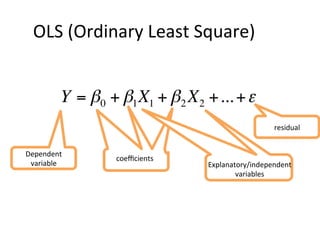
Y = β0 + β1X1 + β2 X2 +...+ε
Dependent	
variable		


coefficients	


Explanatory/independent	
variables	
residual
OLS	(Ordinary	Least	Square)	-	test	
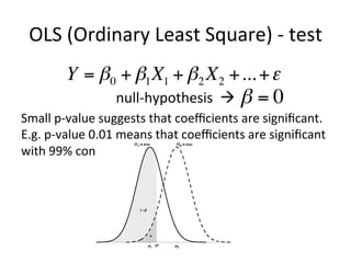
null-hypothesis		à			
Small	p-value	suggests	that	coefficients	are	significant.	
E.g.	p-value	0.01	means	that	coefficients	are	significant	
with	99%	confidence	interval.	
	
	
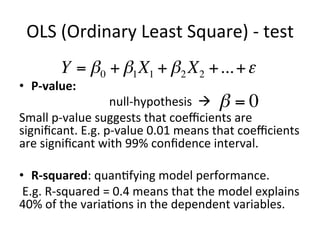
Y = β0 + β1X1 + β2 X2 +...+ε
β = 0
OLS	(Ordinary	Least	Square)	-	test	
•  P-value:		
null-hypothesis		à			
Small	p-value	suggests	that	coefficients	are	
significant.	E.g.	p-value	0.01	means	that	coefficients	
are	significant	with	99%	confidence	interval.	
	
•  R-squared:	quan=fying	model	performance.	
	E.g.	R-squared	=	0.4	means	that	the	model	explains	
40%	of	the	varia=ons	in	the	dependent	variables.	
Y = β0 + β1X1 + β2 X2 +...+ε
β = 0
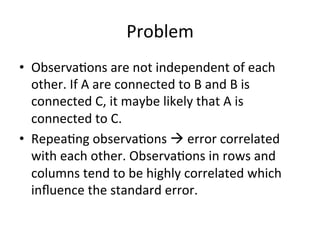
Problem		
•  Observa=ons	are	not	independent	of	each	
other.	If	A	are	connected	to	B	and	B	is	
connected	C,	it	maybe	likely	that	A	is	
connected	to	C.	
•  Repea=ng	observa=ons	à	error	correlated	
with	each	other.	Observa=ons	in	rows	and	
columns	tend	to	be	highly	correlated	which	
influence	the	standard	error.
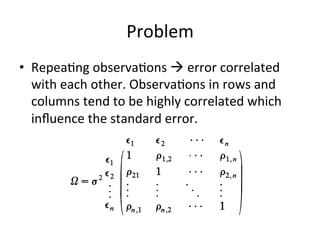
Problem		
•  Repea=ng	observa=ons	à	error	correlated	
with	each	other.	Observa=ons	in	rows	and	
columns	tend	to	be	highly	correlated	which	
influence	the	standard	error.
What	does	QAP	do?	
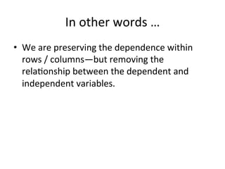
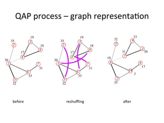
•  Essen=ally,	what	the	QAP	does	is	to	“scramble”	
the	dependent	variable	data	through	several	
permuta?ons.		By	taking	the	data,	and	
“scrambling”	it	repeatedly,	resul=ng	in	mul=ple	
random	datasets	with	the	dependent	variable—
and	then	mul=ple	analyses	can	be	performed.	
•  Those	datasets	and	analyses	form	an	empirical	
sampling	distribu=on,	and	we	can	compare	our	
coefficient	with	this	sampling	distribu?on	of	
coefficients	from	all	the	permuted	datasets.
In	other	words	…	
•  We	are	preserving	the	dependence	within	
rows	/	columns—but	removing	the	
rela=onship	between	the	dependent	and	
independent	variables.
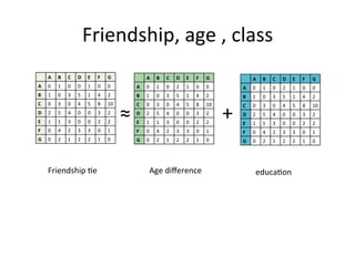
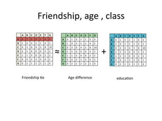
Friendship,	age	,	class	
A	 B	 C	 D	 E	 F	 G	
A	 0	 1	 0	 0	 1	 0	 0	
B	 1	 0	 3	 5	 1	 4	 2	
C	 0	 3	 0	 4	 5	 8	 10	
D	 2	 5	 4	 0	 0	 3	 2	
E	 1	 1	 3	 0	 0	 2	 2	
F	 0	 4	 2	 3	 3	 0	 1	
G	 0	 2	 1	 2	 2	 1	 0	
A	 B	 C	 D	 E	 F	 G	
A	 0	 1	 0	 2	 1	 0	 0	
B	 1	 0	 3	 5	 1	 4	 2	
C	 0	 3	 0	 4	 5	 8	 10	
D	 2	 5	 4	 0	 0	 3	 2	
E	 1	 1	 3	 0	 0	 2	 2	
F	 0	 4	 2	 3	 3	 0	 1	
G	 0	 2	 1	 2	 2	 1	 0	
A	 B	 C	 D	 E	 F	 G	
A	 0	 1	 0	 2	 1	 0	 0	
B	 1	 0	 3	 5	 1	 4	 2	
C	 0	 3	 0	 4	 5	 8	 10	
D	 2	 5	 4	 0	 0	 3	 2	
E	 1	 1	 3	 0	 0	 2	 2	
F	 0	 4	 2	 3	 3	 0	 1	
G	 0	 2	 1	 2	 2	 1	 0	
≈	 +	
Friendship	=e	 Age	difference	 educa=on
A	 B	 C	 D	 E	 F	 G	
A	 0	 1	 0	 0	 1	 0	 0	
B	 1	 0	 3	 5	 1	 4	 2	
C	 0	 3	 0	 4	 5	 8	 10	
D	 2	 5	 4	 0	 0	 3	 2	
E	 1	 1	 3	 0	 0	 2	 2	
F	 0	 4	 2	 3	 3	 0	 1	
G	 0	 2	 1	 2	 2	 1	 0	
A	 B	 C	 D	 E	 F	 G	
A	 0	 1	 0	 2	 1	 0	 0	
B	 1	 0	 3	 5	 1	 4	 2	
C	 0	 3	 0	 4	 5	 8	 10	
D	 2	 5	 4	 0	 0	 3	 2	
E	 1	 1	 3	 0	 0	 2	 2	
F	 0	 4	 2	 3	 3	 0	 1	
G	 0	 2	 1	 2	 2	 1	 0	
A	 B	 C	 D	 E	 F	 G	
A	 0	 1	 0	 2	 1	 0	 0	
B	 1	 0	 3	 5	 1	 4	 2	
C	 0	 3	 0	 4	 5	 8	 10	
D	 2	 5	 4	 0	 0	 3	 2	
E	 1	 1	 3	 0	 0	 2	 2	
F	 0	 4	 2	 3	 3	 0	 1	
G	 0	 2	 1	 2	 2	 1	 0	
≈	 +	
Friendship	=e	 Age	difference	 educa=on	
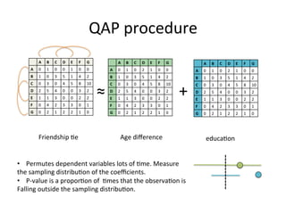
•  Permutes	dependent	variables	lots	of	=me.	Measure	
the	sampling	distribu=on	of	the	coefficients.			
•  P-value	is	a	propor=on	of		=mes	that	the	observa=on	is	
Falling	outside	the	sampling	distribu=on.	
QAP	procedure
QAP	process	–	graph	representa=on	
before	 reshuffling	 ajer
Available	func=ons	
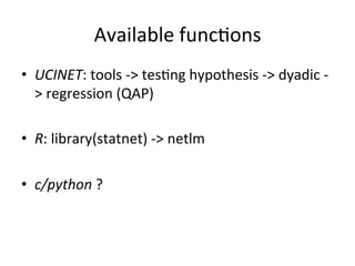
•  UCINET:	tools	->	tes=ng	hypothesis	->	dyadic	-
>	regression	(QAP)	
	
•  R:	library(statnet)	->	netlm	
	
•  c/python	?
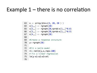
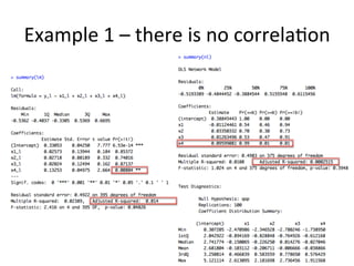
Example	1	–	there	is	no	correla=on
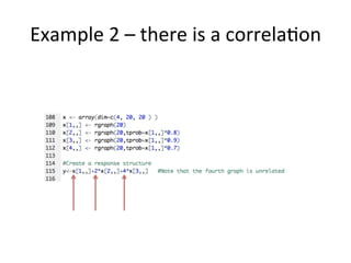
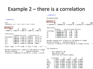
Example	2	–	there	is	a	correla=on
Recap		
•  QAP	is	useful	when	we	have	dyadic	
rela=onship	in	the	data.	
•  Use	netlm	func=on	in	R	for	the	regression	
analysis.	
•  Disadvantage:	it	is	slow	for	large	network	size
References	
•  Predic=ng	with	networks:	nonparametric	
mul=ple	regression	analysis	of	dyadic	data,	D.	
Krackhardt	(1981)	
•  The	SNA	package,	CT	Buos	(2014)	
•  hop://svitsrv25.epfl.ch/R-doc/library/sna/html/
qaptest.html	
•  hop://www.stata.com/mee=ng/1nasug/
simpson.pdf	
•  hop://www.erikgjesqeld.net/uploads/
3/7/6/8/37685481/
sna_code_(gjesqeld_and_phillips_2013).pdf