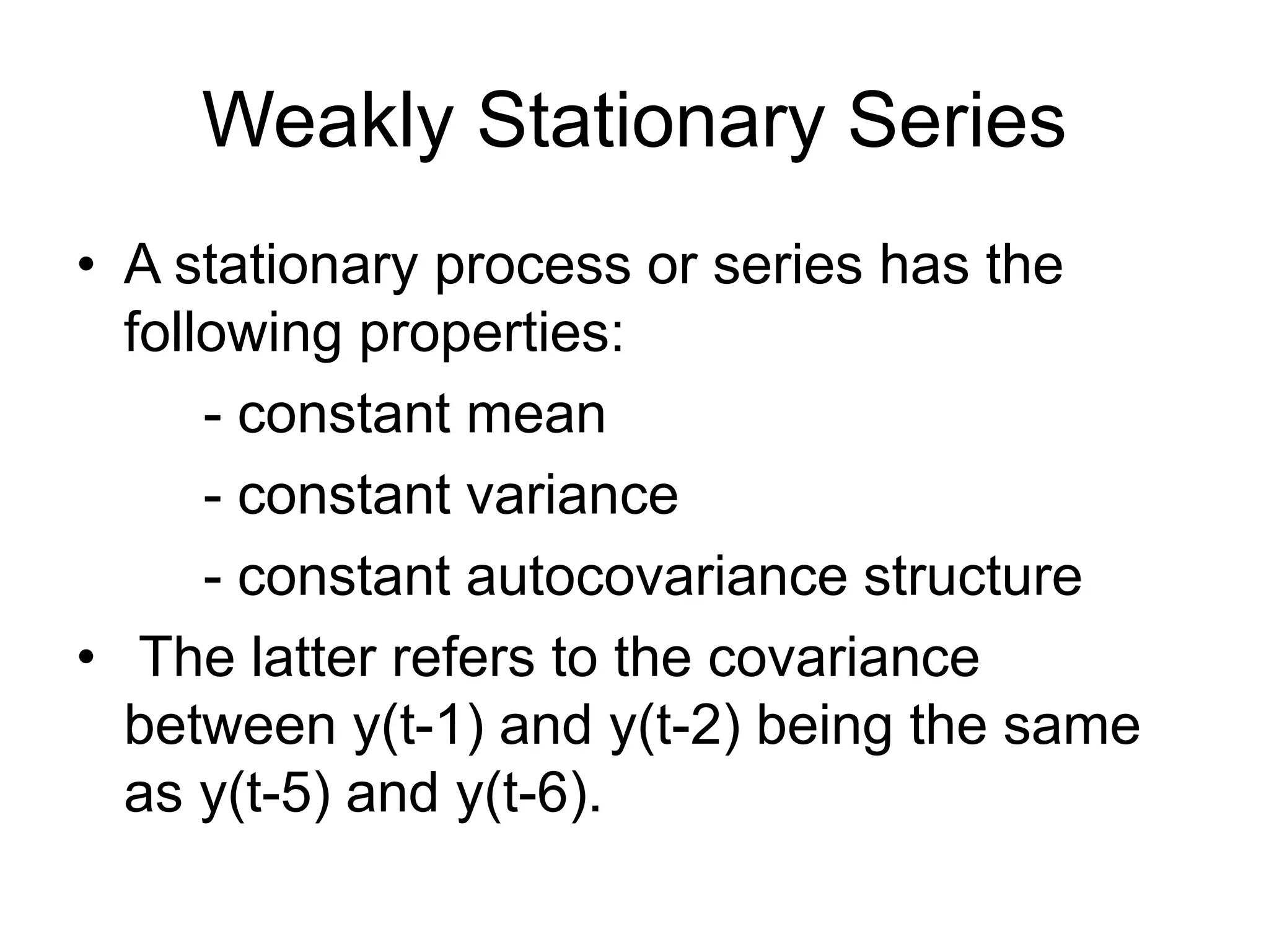
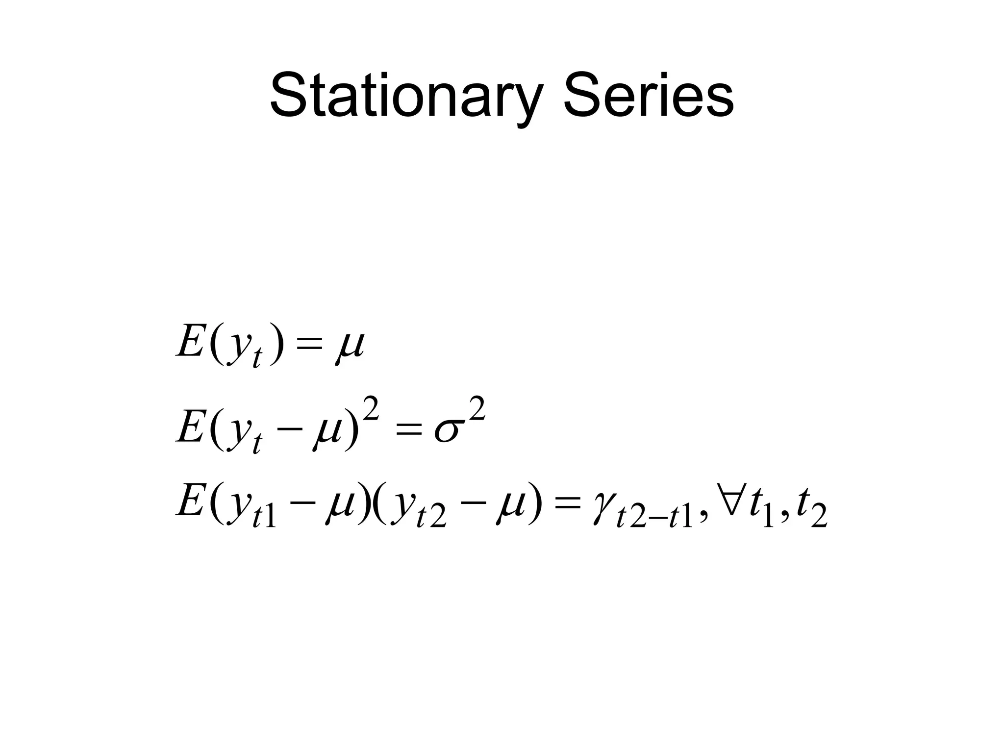
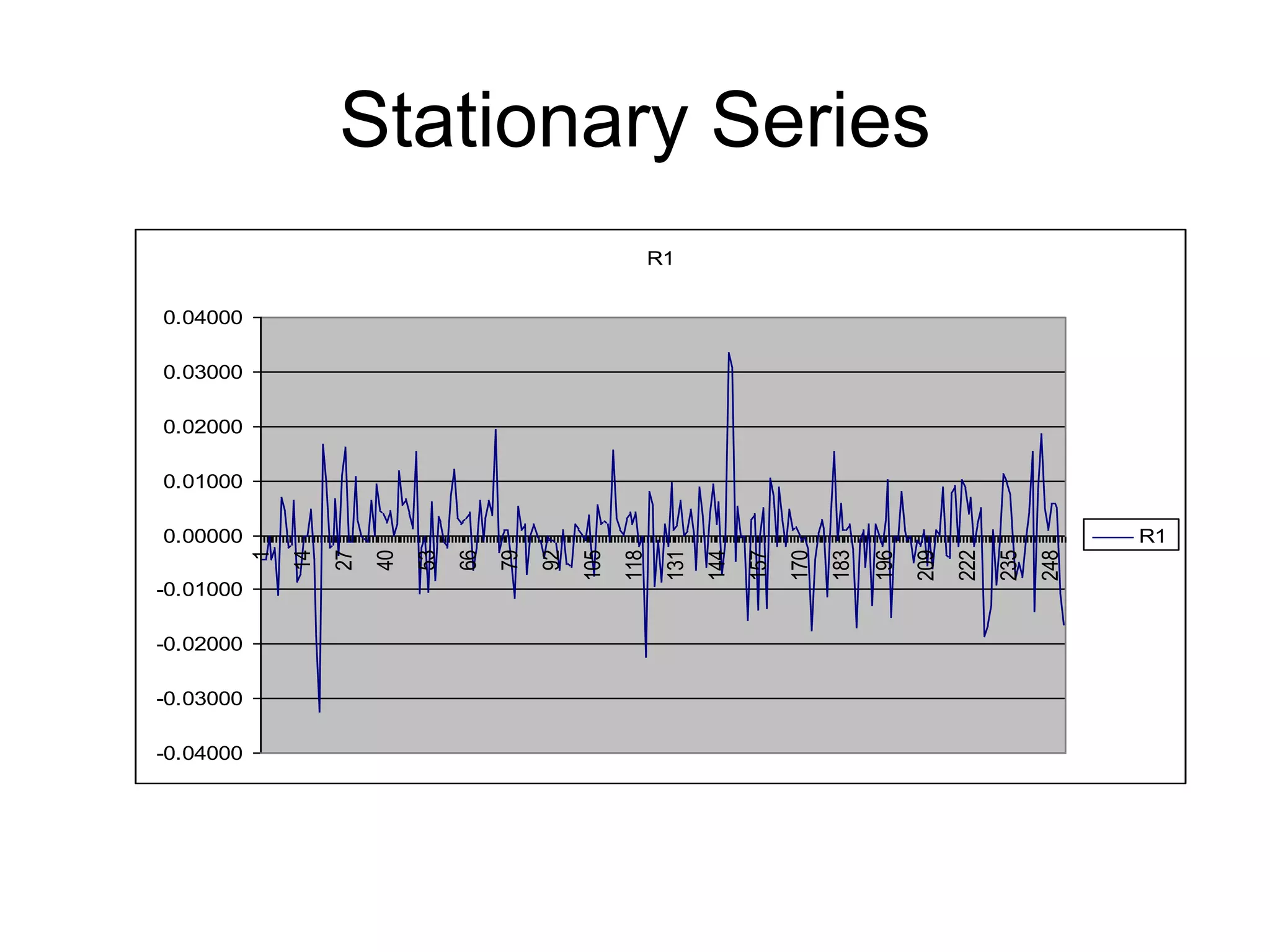
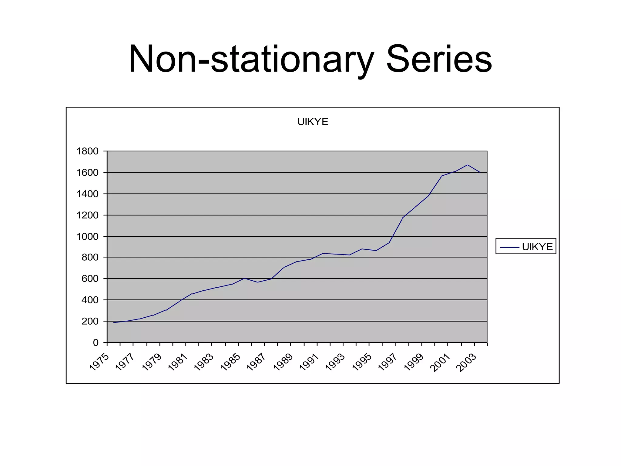
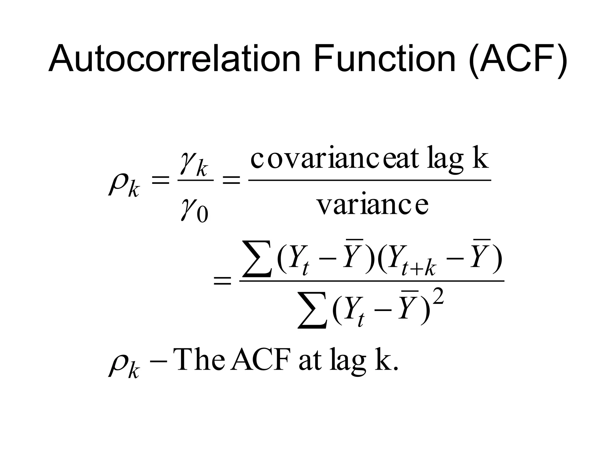
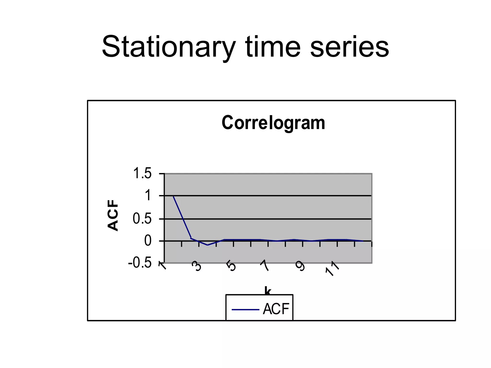
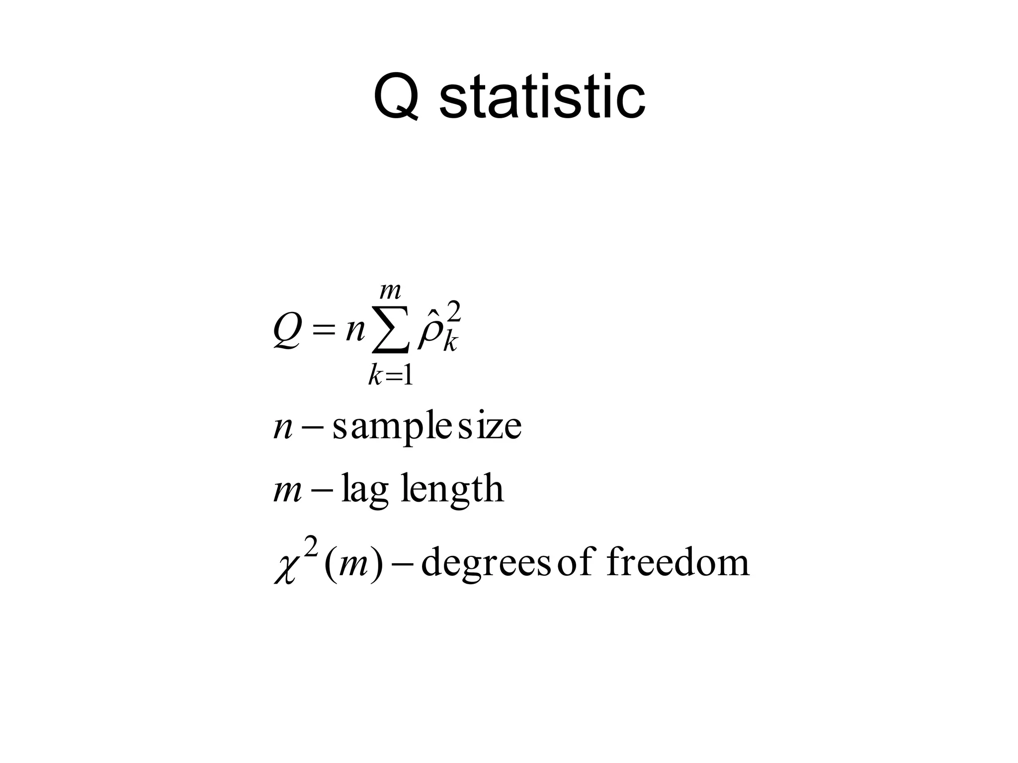
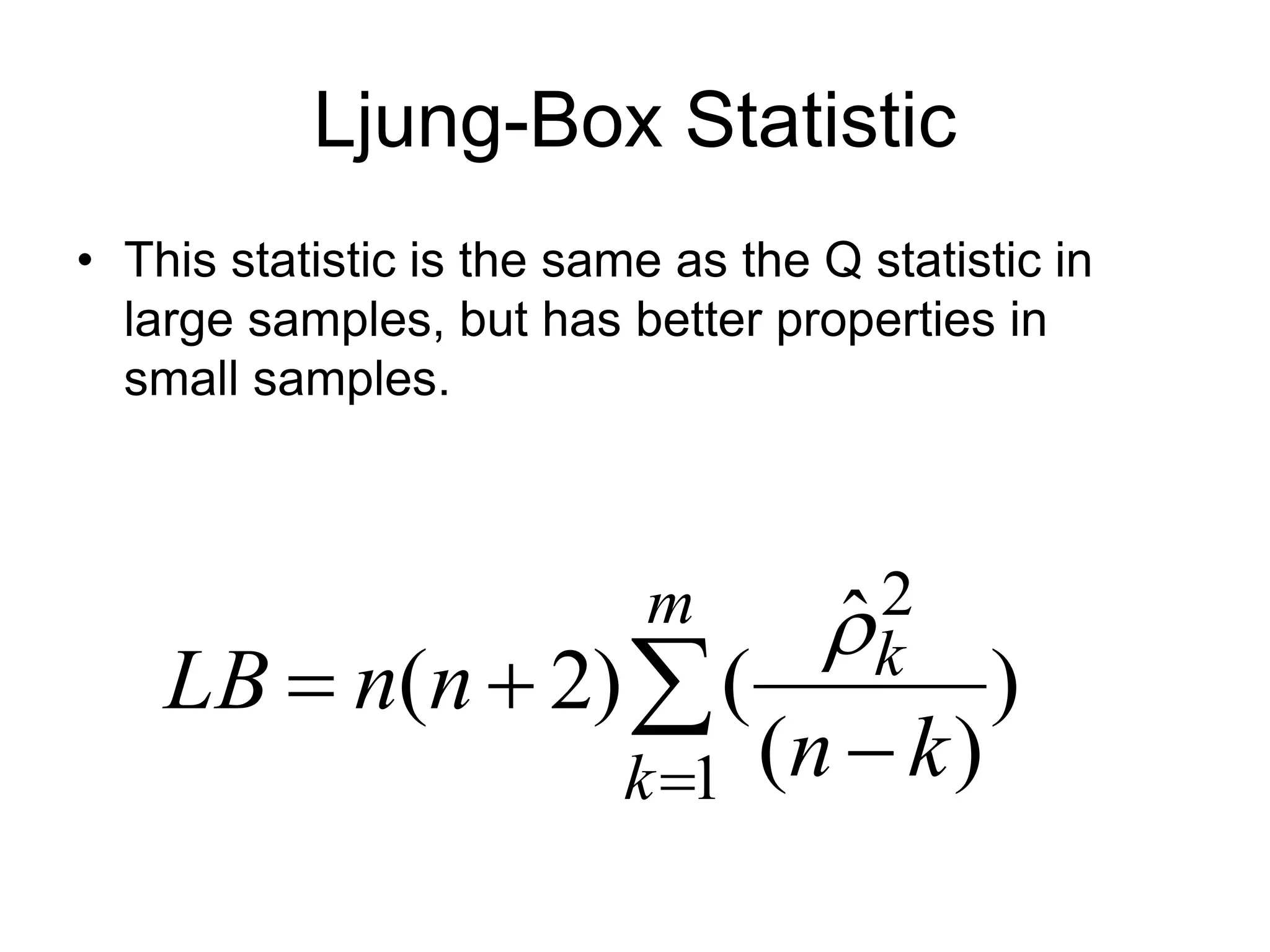
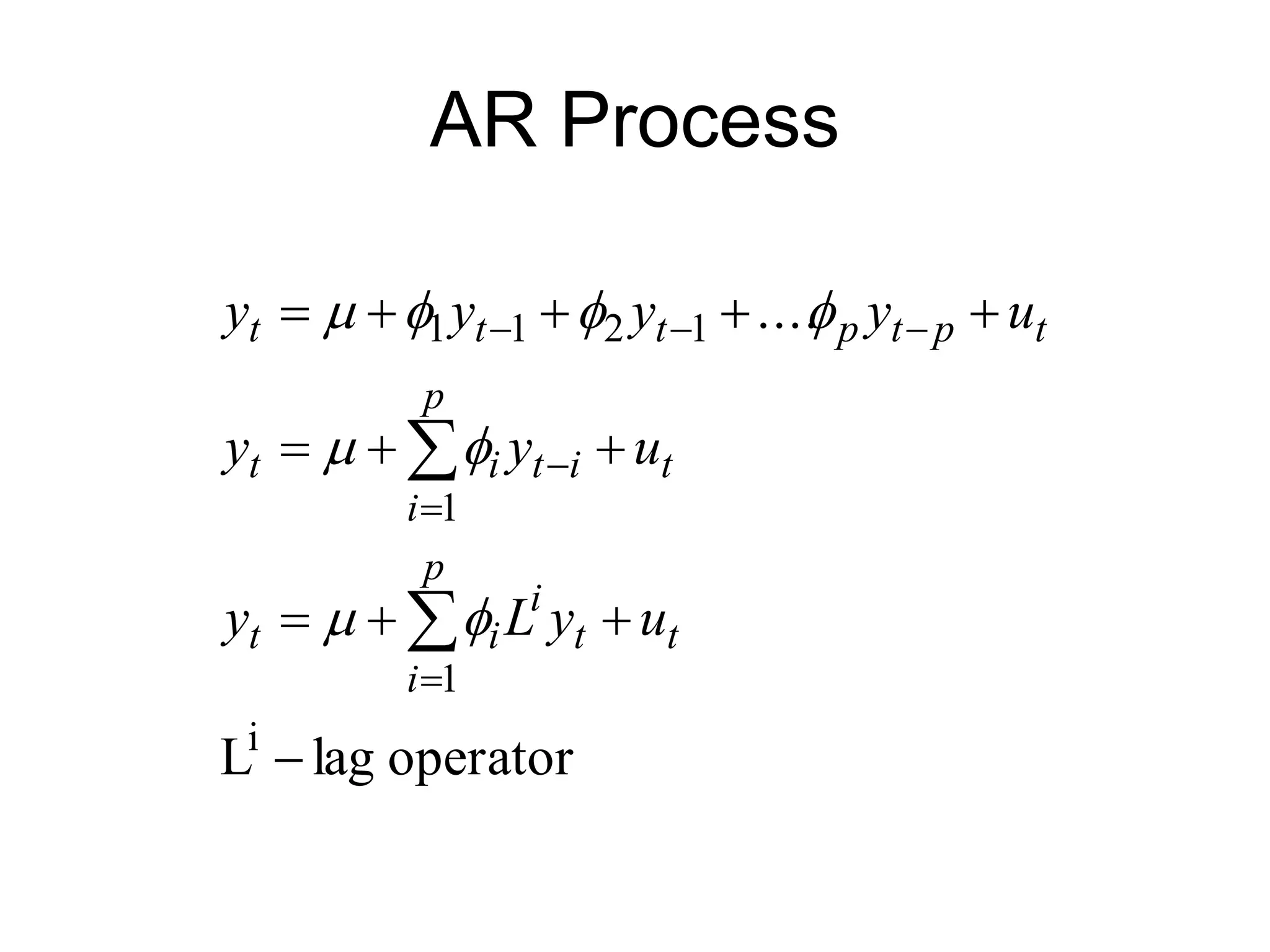
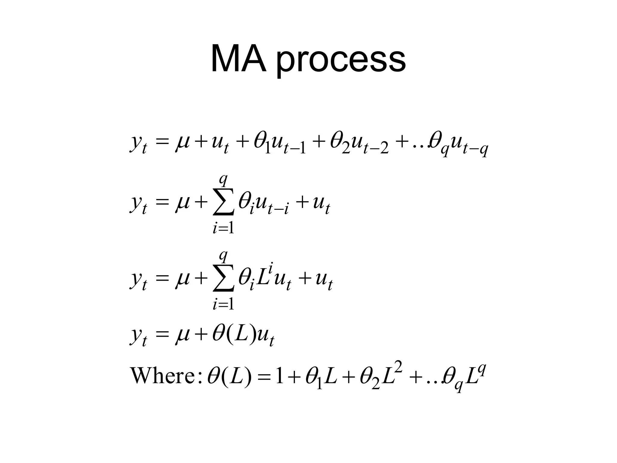
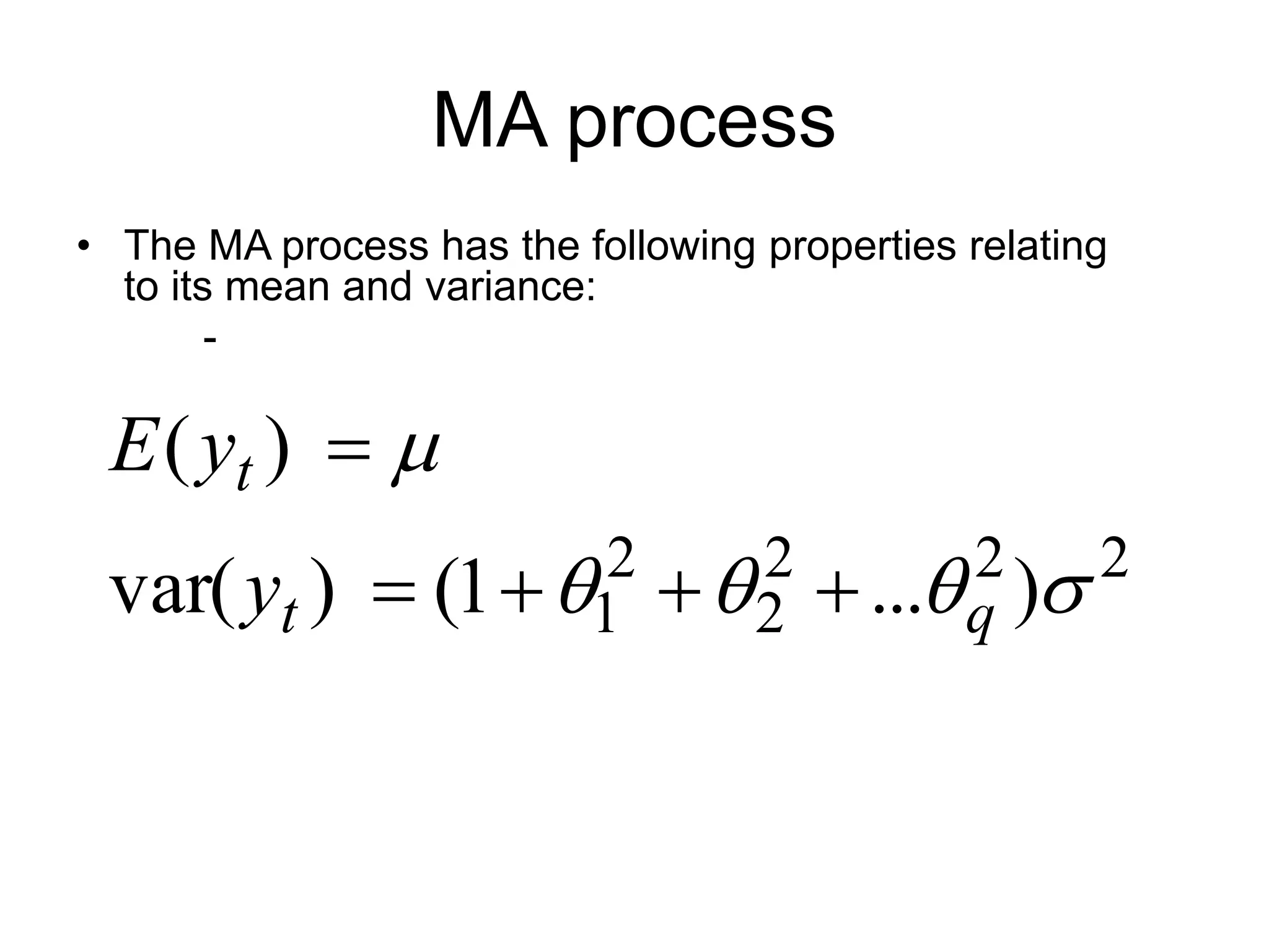
This document discusses stationarity, autocorrelation functions, and autoregressive integrated moving average (ARIMA) models. It defines stationarity and describes autocorrelation coefficients and the Q-statistic for evaluating stationarity. The components of an ARIMA model are autoregressive (AR) processes involving lagged dependent variables and moving average (MA) processes involving lagged error terms. The document provides examples of AR and MA processes and discusses interpreting their coefficients.

1. Autocorrelation Functions and
ARIMA Modelling

2. Introduction
• Define what stationarity is and why it is so
important to Econometrics
• Describe the Autocorrelation coefficient
and its relationship to stationarity
• Evaluate the Q-statistic
• Describe the components of an
Autoregressive Integrated Moving Average
Model (ARIMA model)

3. Stationarity
• A strictly stationary process is one where
the distribution of its values remains the
same as time proceeds, implying that the
probability lies in a particular interval is the
same now as at any point in the past or
the future.
• However we tend to use the criteria
relating to a ‘weakly stationary process’ to
determine if a series is stationary or not.

4. Weakly Stationary Series
• A stationary process or series has the
following properties:
- constant mean
- constant variance
- constant autocovariance structure
• The latter refers to the covariance
between y(t-1) and y(t-2) being the same
as y(t-5) and y(t-6).

5. Stationary Series
2
1
1
2
2
1
2
2
,
,
)
)(
(
)
(
)
(
t
t
y
y
E
y
E
y
E
t
t
t
t
t
t















6. Stationary Series
R1
-0.04000
-0.03000
-0.02000
-0.01000
0.00000
0.01000
0.02000
0.03000
0.04000
1
14
27
40
53
66
79
92
105
118
131
144
157
170
183
196
209
222
235
248
R1

7. Non-stationary Series
UIKYE
0
200
400
600
800
1000
1200
1400
1600
1800
1
9
7
5
1
9
7
7
1
9
7
9
1
9
8
1
1
9
8
3
1
9
8
5
1
9
8
7
1
9
8
9
1
9
9
1
1
9
9
3
1
9
9
5
1
9
9
7
1
9
9
9
2
0
0
1
2
0
0
3
UIKYE

8. Implications of Non-stationary data
• If the variables in an OLS regression are
not stationary, they tend to produce
regressions with high R-squared statistics
and low DW statistics, indicating high
levels of autocorrelation.
• This is caused by the drift in the variables
often being related, but not directly
accounted for in the regression, hence the
omitted variable effect.

9. Stationary Data
• It is important to determine if our data is
stationary before the regression. This can
be done in a number of ways:
- plotting the data
- assessing the autocorrelation function
- Using a specific test on the
significance of the autocorrelation
coefficients.
- Specific tests to be covered later.

10. Autocorrelation Function (ACF)
k.
lag
at
ACF
The
)
(
)
)(
(
variance
k
lag
at
covariance
2
0








 
k
t
k
t
t
k
k
Y
Y
Y
Y
Y
Y





11. Correlogram
• The sample correlogram is the plot of the ACF
against k.
• As the ACF lies between -1 and +1, the
correlogram also lies between these values.
• It can be used to determine stationarity, if the
ACF falls immediately from 1 to 0, then equals
about 0 thereafter, the series is stationary.
• If the ACF declines gradually from 1 to 0 over a
prolonged period of time, then it is not stationary.

12. Stationary time series
Correlogram
-0.5
0
0.5
1
1.5
1
3
5
7
9
1
1
k
ACF
ACF

13. Statistical Significance of the ACF
• The Q statistic can be used to determine if
the sample ACFs are jointly equal to zero.
• If jointly equal to zero we can conclude
that the series is stationary.
• It follows the chi-squared distribution,
where the null hypothesis is that the
sample ACFs jointly equal zero.

14. Q statistic
freedom
of
degrees
)
(
length
lag
size
sample
ˆ
2
1
2



 

m
m
n
n
Q
m
k
k



15. Ljung-Box Statistic
• This statistic is the same as the Q statistic in
large samples, but has better properties in
small samples.
)
)
(
ˆ
(
)
2
(
1
2

 


m
k
k
k
n
n
n
LB


16. Partial ACF
• The Partial Autocorrelation Function
(PACF) is similar to the ACF, however it
measures correlation between
observations that are k time periods apart,
after controlling for correlations at
intermediate lags.
• This can also be used to produce a partial
correlogram, which is used in Box-Jenkins
methodology (covered later).

17. Q-statistic Example
• The following information, from a specific
variable can be used to determine if a time
series is stationary or not.
60
32
.
0
ˆ
4
1
2




n
k
k


18. Q-statistic
0.
to
different
tly
significan
jointly
are
ACFs
the
as
stationary
not
is
series
The
488
.
9
2
.
19
488
.
9
)
4
(
2
.
19
32
.
0
*
60
0
2
H
reject
Q








19. Autoregressive Process
• An AR process involves the inclusion of
lagged dependent variables.
• An AR(1) process involves a single lag, an
AR(p) model involves p lags.
• AR(1) processes are often referred to as
the random walk, or driftless random walk
if we exclude the constant.

20. AR Process
operator
lag
L
....
i
1
1
1
2
1
1




















t
t
i
p
i
i
t
t
i
t
p
i
i
t
t
p
t
p
t
t
t
u
y
L
y
u
y
y
u
y
y
y
y









21. Moving Average (MA) process
• In this simple model, the dependent
variable is regressed against lagged
values of the error term.
• We assume that the assumptions on the
mean of the error term being 0 and having
a constant variance etc still apply.

22. MA process
q
q
t
t
t
t
q
i
i
i
t
t
i
t
q
i
i
t
q
t
q
t
t
t
t
L
L
L
L
u
L
y
u
u
L
y
u
u
y
u
u
u
u
y














...
1
)
(
:
Where
)
(
...
2
2
1
1
1
2
2
1
1


























23. MA process
• To estimate moving average processes,
involves interpreting the coefficients and t-
statistics in the usual way
• It is possible to have a model with lags on
the 1st but not 2nd, then 3rd lags. This
produces the problem of how to determine
the optimal number of lags.

24. MA process
• The MA process has the following properties relating
to its mean and variance:
-
2
2
2
2
2
1 )
...
1
(
)
var(
)
(





q
t
t
y
y
E






25. Example of an MA Process
term
error
u
output
y
LM
u
y
y t
t
t
47
.
2
)
1
(
,
15
.
0
R
(0.1)
(0.2)
(0.1)
3
.
0
8
.
0
7
.
0
ˆ
2
1
1






 


26. Example
• In the previous slide we have estimated a
model using an AR(1) process and MA(1)
process or ARMA(1,1) model, with a lag
on the MA part to pick up any inertia in
adjustment in output.
• The t-statistics are interpreted in the same
way, in this case only one MA lag was
significant.

27. Conclusion
• Before conducting a regression, we need to
consider whether the variables are stationary or
not.
• The ACF and correlogram is one way of
determining if a series is stationary, as is the Q-
statistic
• An AR(p) process involves the use of p lags of
the dependent variable as explanatory variables
• A MA(q) process involves the use of q lags of
the error term.