Downloaded 704 times
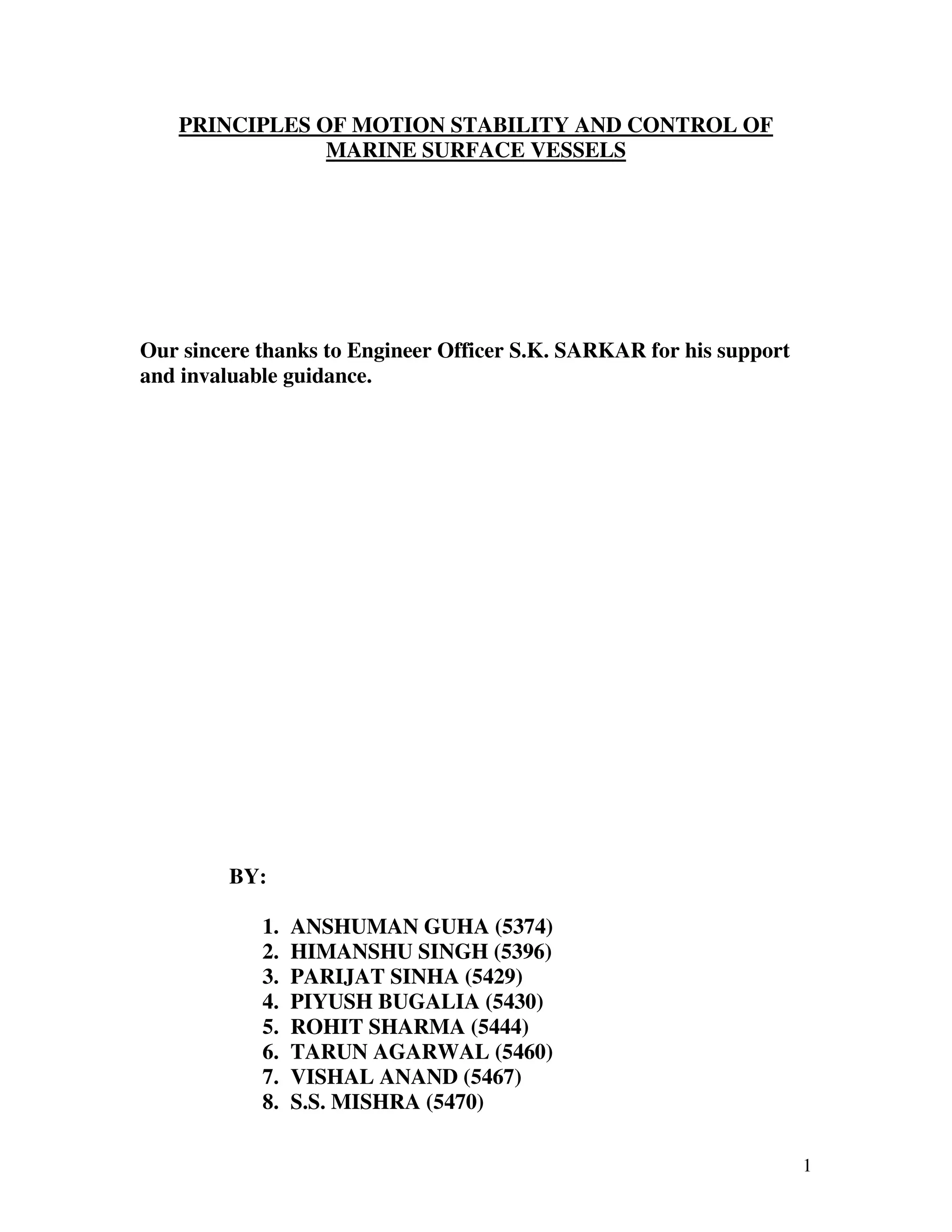
![X = X 0 cosψ + Y0 sinψ
Y = Y0 cosψ − X 0 sinψ − − − − − − − − − −(2)
likewise
x0G = u cosψ + v sinψ
&
y 0G = v cosψ − u cosψ − − − − − − − − − − − (3)
&
then
&&0G = u cosψ − v sin ψ − (u sin ψ + v sin ψ )ψ
x & &
&&0G = u sin ψ + v cosψ + (u cosψ − v sin ψ )ψ − − − − − − − (4)
y & &
Substituting equation (4) in equation (1) and inserting the resulting values of Xo and Yo
in equation (2) yields the simple expressions:
X = m(u − vψ )
& &
Y = m ( v + uψ )
& &
For completeness:
X = m(u − vψ ) − − − − − − − − surge
&
Y = m(v + uψ ) − − − − − − − − sway − − − − − −(5)
&
N = I zψ& − − − − − − − − − − − yaw
&
Note the existence of the term muψ in the equation of Y and mvψ .In the equation for
& &
X, whereas terms like these are not present in equation (1). These are the so-called
centrifugal force terms which exist when systems with moving axes are considered, but
do not exist when the axes are fixed in the earth.
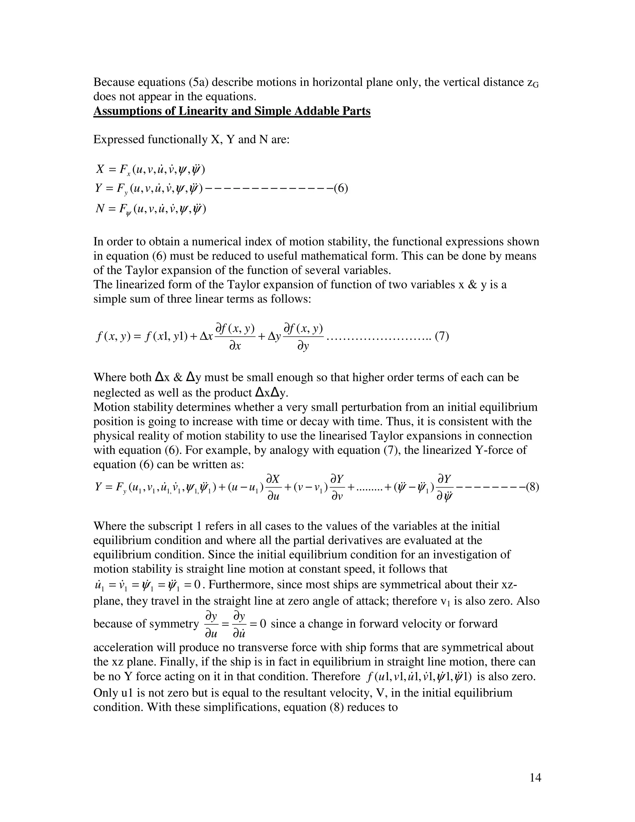
Equations (5) have been developed for the case where the origin of the axes, O, is at the
C.G. of the ship. Suppose we chose an origin, O, which is located a distance RG from the
CG of the ship, where RG has components xG, yG and zG along the x,y and z axes which
are parallel to the principal axes of inertia through G. xG will be positive if the CG is
forward of the origin and negative if it is aft. Similarly yG will be positive if G is to
starboard of O and zG will be positive if G is below O. Abkowitz has shown that for the
choice of position for the origin, equations (5) become:
X = m(u − ψv − y Gψ& − xGψ 2 )
& &
Y = m(v + uψ − y Gψ 2 + xGψ&) − − − − − − − − − − − − − − − − − (5a )
& &
N = I zψ& + m[ xG (v + uψ ) − y G (u − ψv)]
& & &
13](https://image.slidesharecdn.com/final1-091028042342-phpapp02/75/Motion-stability-and-control-in-marine-surface-vessels-13-2048.jpg)
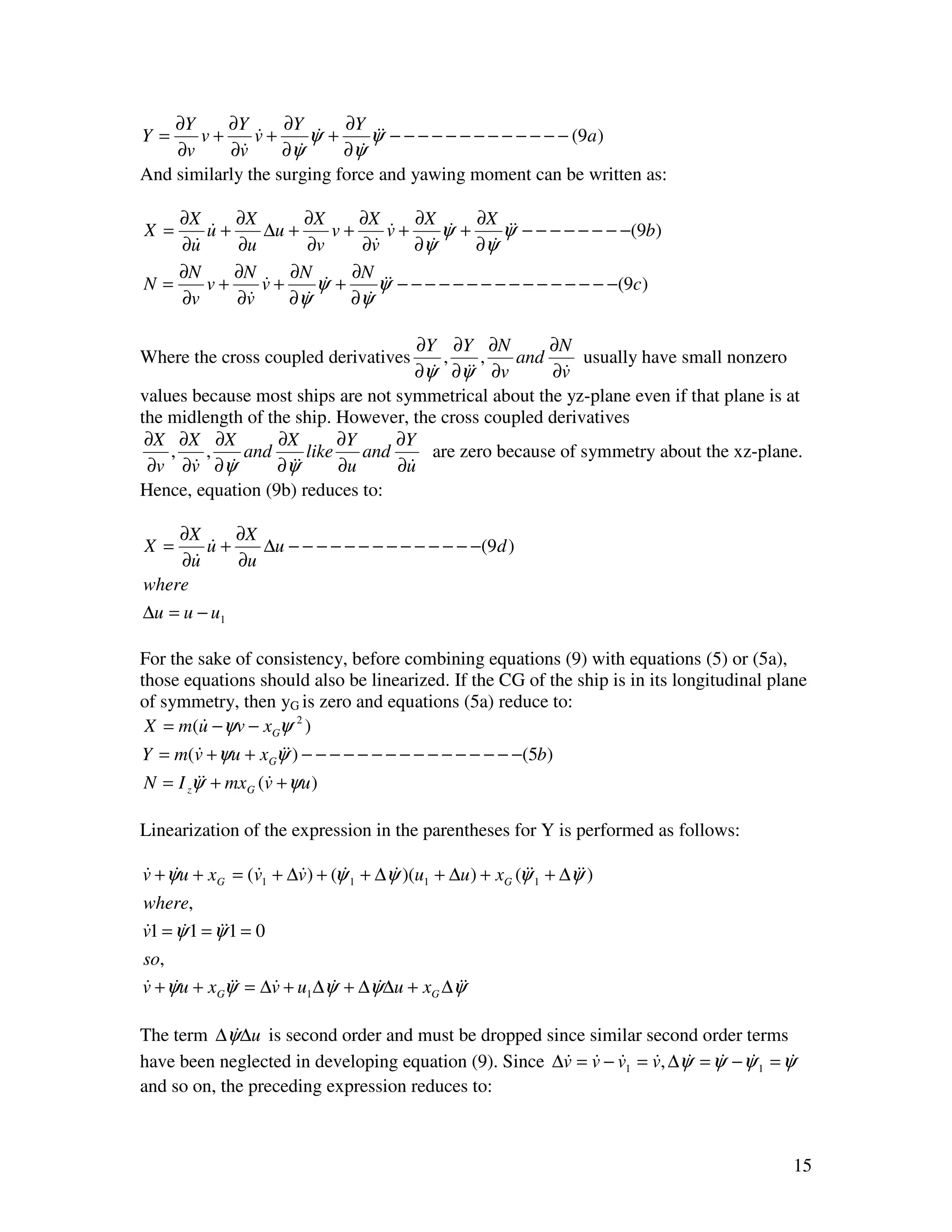
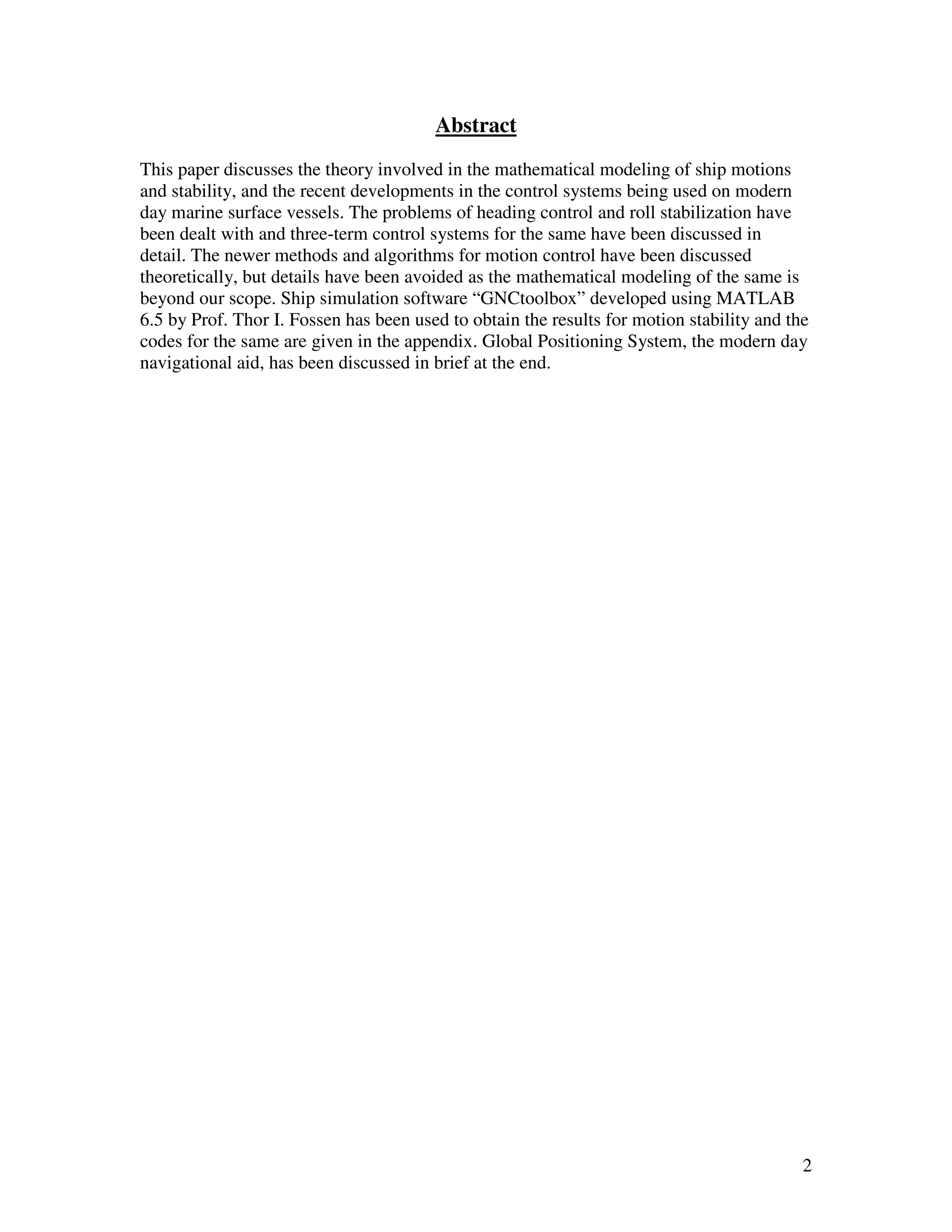
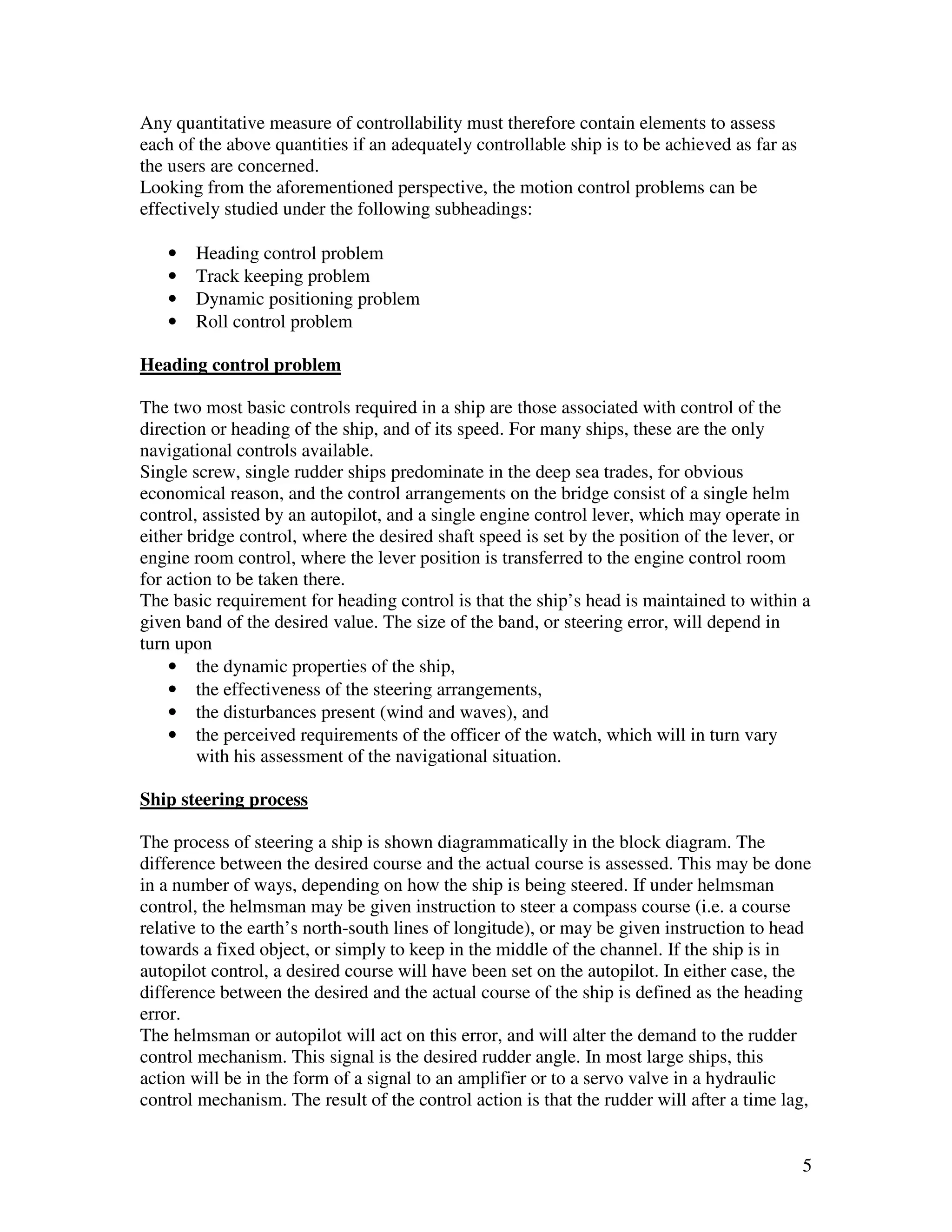
![where t is the time lag of the control system.
Following equation (7) the linearized form of the Taylor expansion of equation (15) is
δ (t ) = k1 [ψ (t ) − tψ (t )] + k 2 [ψ (t ) − tψ&(t )]
& & &
Nondimensionalizing this equation, substituting it in equation (11a), and dropping the
functional notation (t) which is implicit in equation (11a), the following is obtained:
Yv′v ′ + (Yv&′ − m ′)v ′ + k1Yδ′ψ + (Yψ′ − m′ + k 2Yδ′ − k1 t ′Yδ′ )ψ ′ + (Yψ′& − m′xG − k 2 t ′Yδ′ )ψ&′ = 0
& & & ′ &
N v v ′ + ( N v& − m′xG )v ′ + k1 N δψ + ( Nψ& − m′xG + k 2 N δ − k1 t N ′δ )ψ ′ + ( Nψ& − I z − k 2 t ′N δ )ψ&′ = 0
′ ′ ′ & ′ ′ ′ & ′& ′ ′ &
Where t ′ = (t )(V / L)
Again comparing with criterion, C, equation (12), it is noted that the term (Yr′ − m′) now
appears as (Yr′ − m′ + k 2Yδ′ − k1 t ′Yδ′ ) and the term ( N r′ − m′xG ) appears as
′
( N r′ − m′xG + k 2 N δ − k1 t ′N δ ) .
′ ′ ′
Two important facts emerge from these comparisons:
• The existence of the time lag, t , detracts from the stability of the ship compared
to zero time lag.
• If automatic controls were made sensitive only toψ , and not toψ , (k2=0) and a
&
time lag existed, the stability of the ships with controls would be less than
without controls. It is conceivable that this decrease in stability could cause a
ship that was stable without controls to become unstable with controls.
A more accurate and realistic, but much more complicate, analysis of the lags in the
control systems can be accomplished by writing the equations which describe the actual
operation of the various mechanisms involved in the system. For example, the equation
describing the build-up of voltage (or amperage) as a function of the quantitiesψandψ , &
the equations describing the actual method of amplification of the signal to produce the
power to activate the rudder motor, the equations describing the electromechanical
response of the electric motor activating the rudder system and the equations of motion of
the rudder system itself can all be written. These equations can then be coupled with the
ship motion equations and the overall response analyzed. The results will give a complete
test of the stability of the overall system, ship and controls. The controls themselves can,
as shown earlier, introduce instability into the system if they are not properly designed.
One solution proposed to remove the time lag from the system is to use some form of
ship-board sensor to determine the presence of disturbances like a large wave. This could
be achieved by some form of laser based device which would be aligned up weather, and
used to sense the presence of a wave or disturbance some seconds before it strikes the
ship.
20](https://image.slidesharecdn.com/final1-091028042342-phpapp02/75/Motion-stability-and-control-in-marine-surface-vessels-20-2048.jpg)
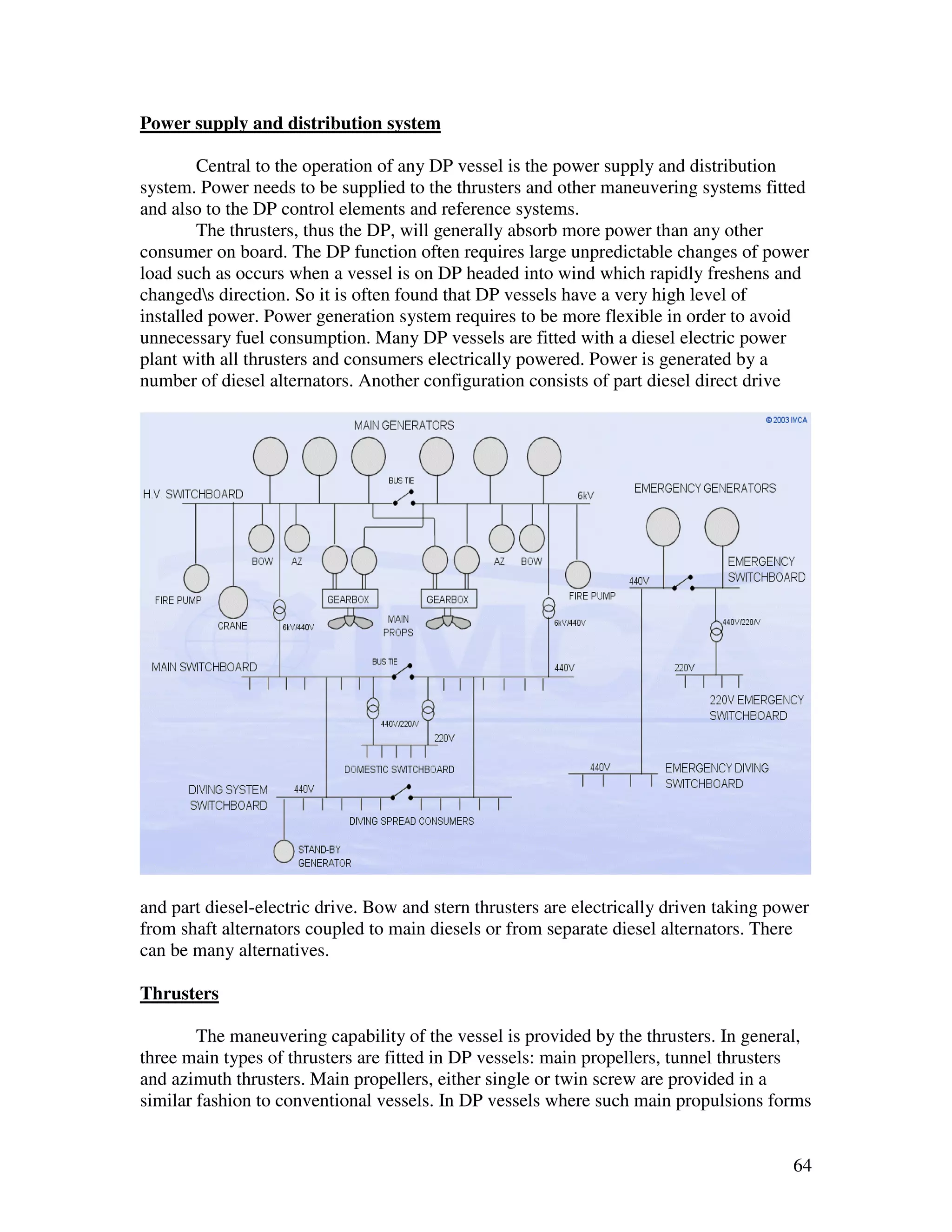
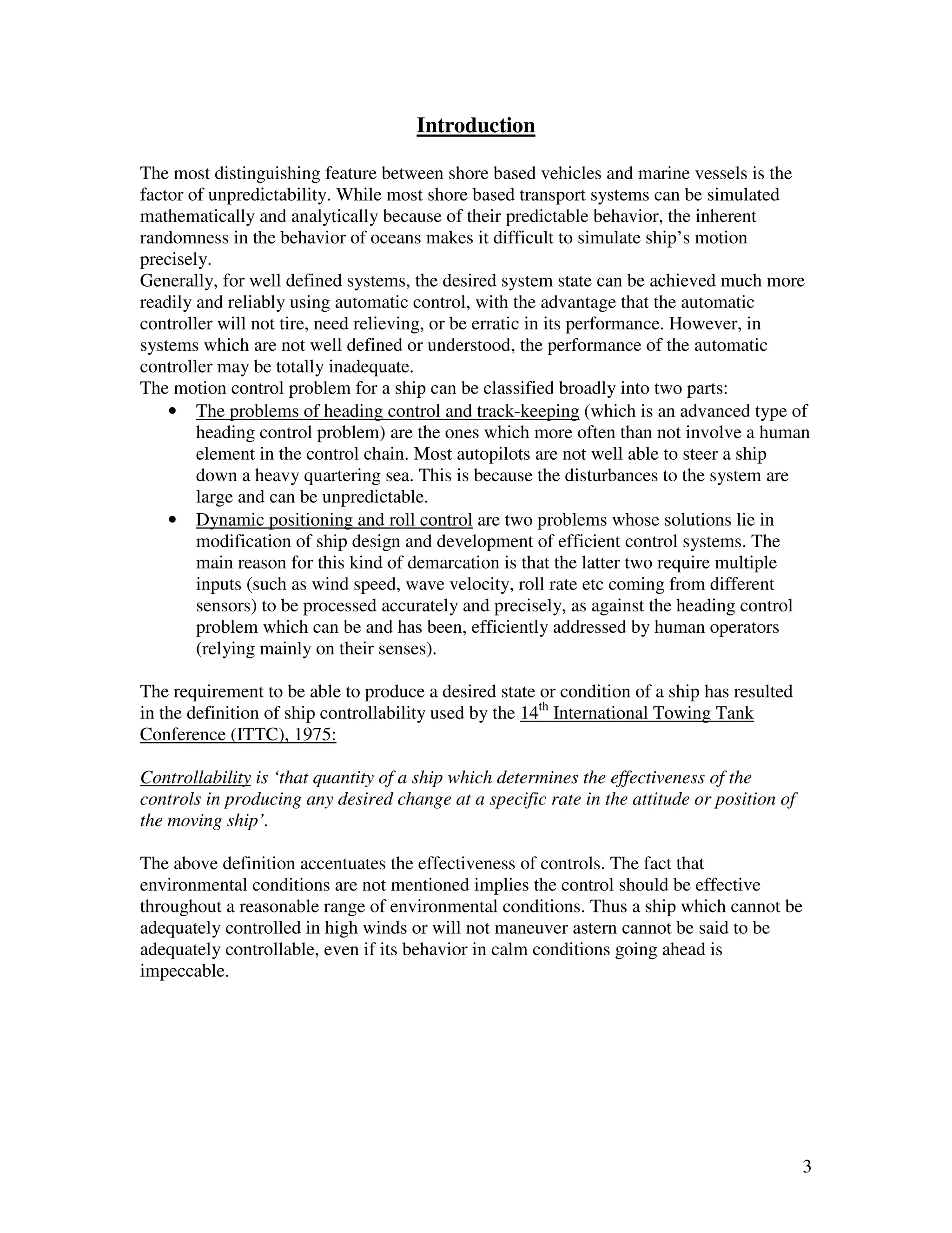
![part of the DP function propellers are usually controllable pitch running at
constant rpm. This facilitates the use of shaft driven alternators as these could not be used
if the shaft drive is not at constant rpm; the DP function is not best served by fixed pitch
propellers continually starting, stopping and reversing, particularly if the power source is
direct drive diesel. Main propellers are usually accompanied by conventional rudders and
steering gear. Generally (though not exclusively) the DP system does not include rudder
control; the autopilot being disconnected and the rudder set amidships when in DP mode.
DP Control Modeling
Dynamic positioning of floating vessels is a technique for maintaining the position and
heading of the vessel without the use of mooring system [1]. In a conventional floating
vessel the forces required to overcome the effects of wind, waves and current are
provided by the mooring system. The most significant limitation of that solution is the
difficulty of mooring in deep water. In fact, at some water depth the multipoint mooring
system is totally impractical. In a dynamically positioned vessel the forces are provided
by thrust devices.
65](https://image.slidesharecdn.com/final1-091028042342-phpapp02/75/Motion-stability-and-control-in-marine-surface-vessels-65-2048.jpg)
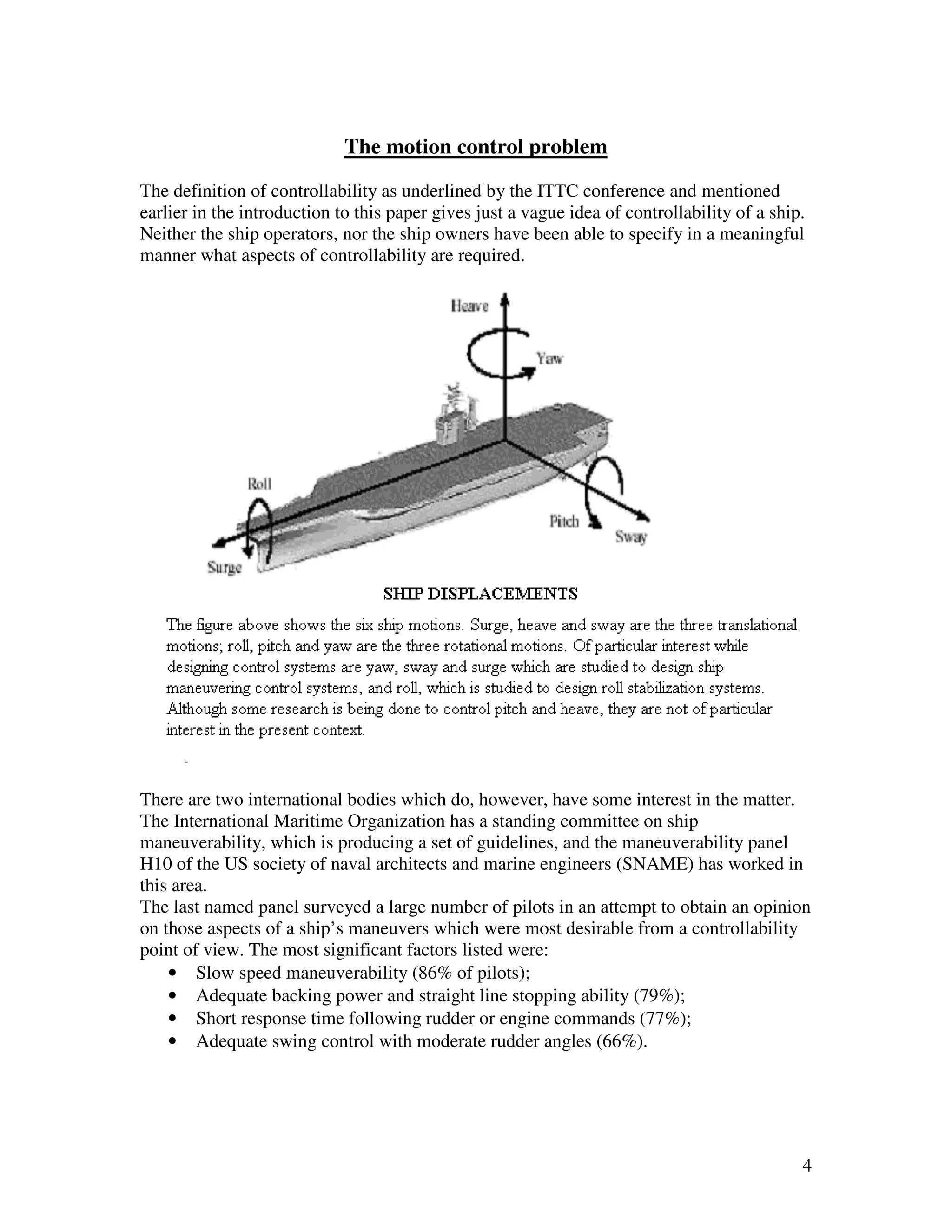
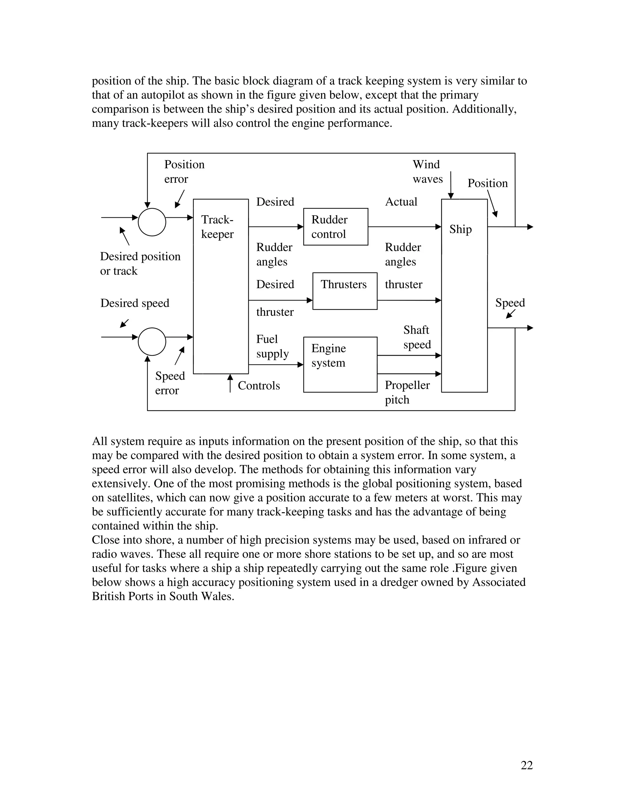
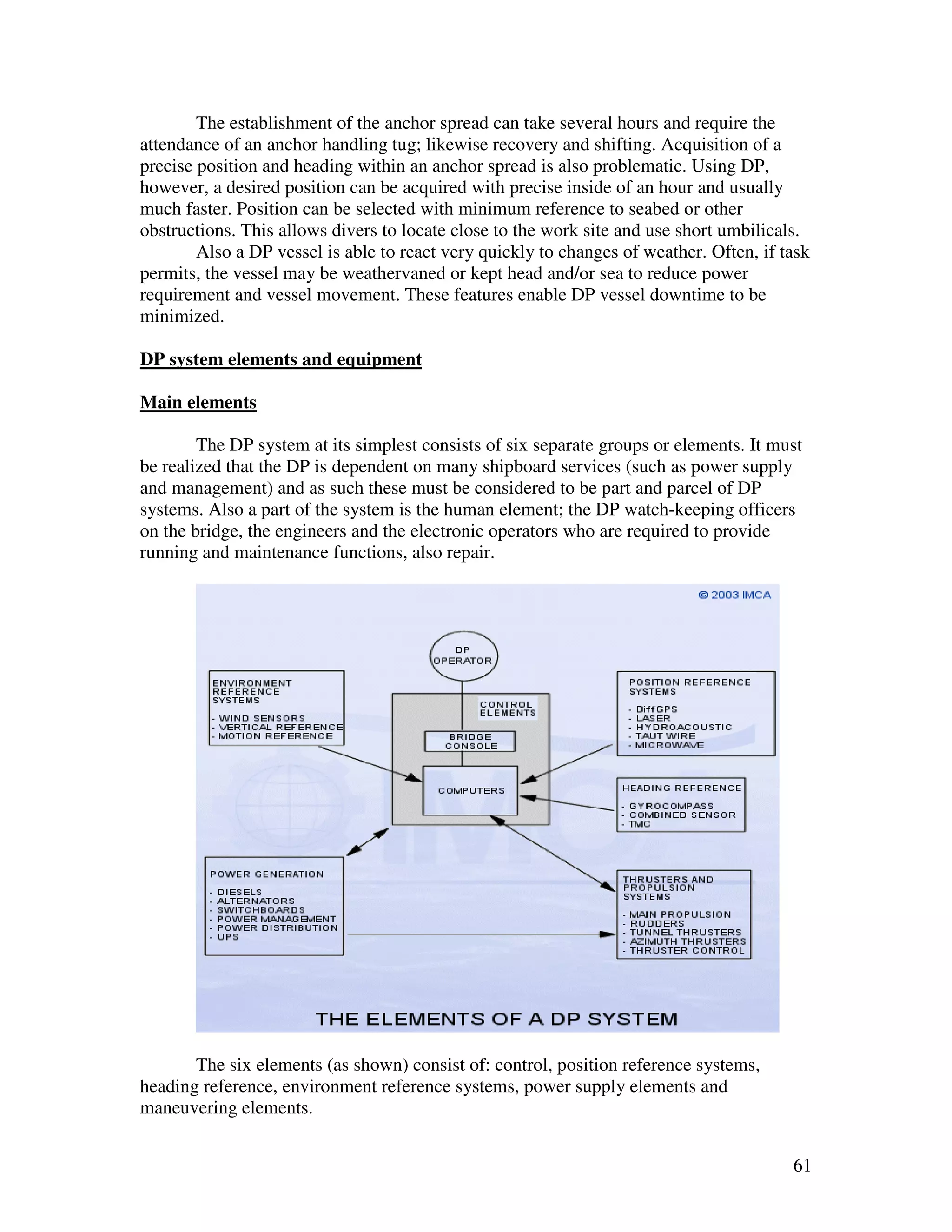
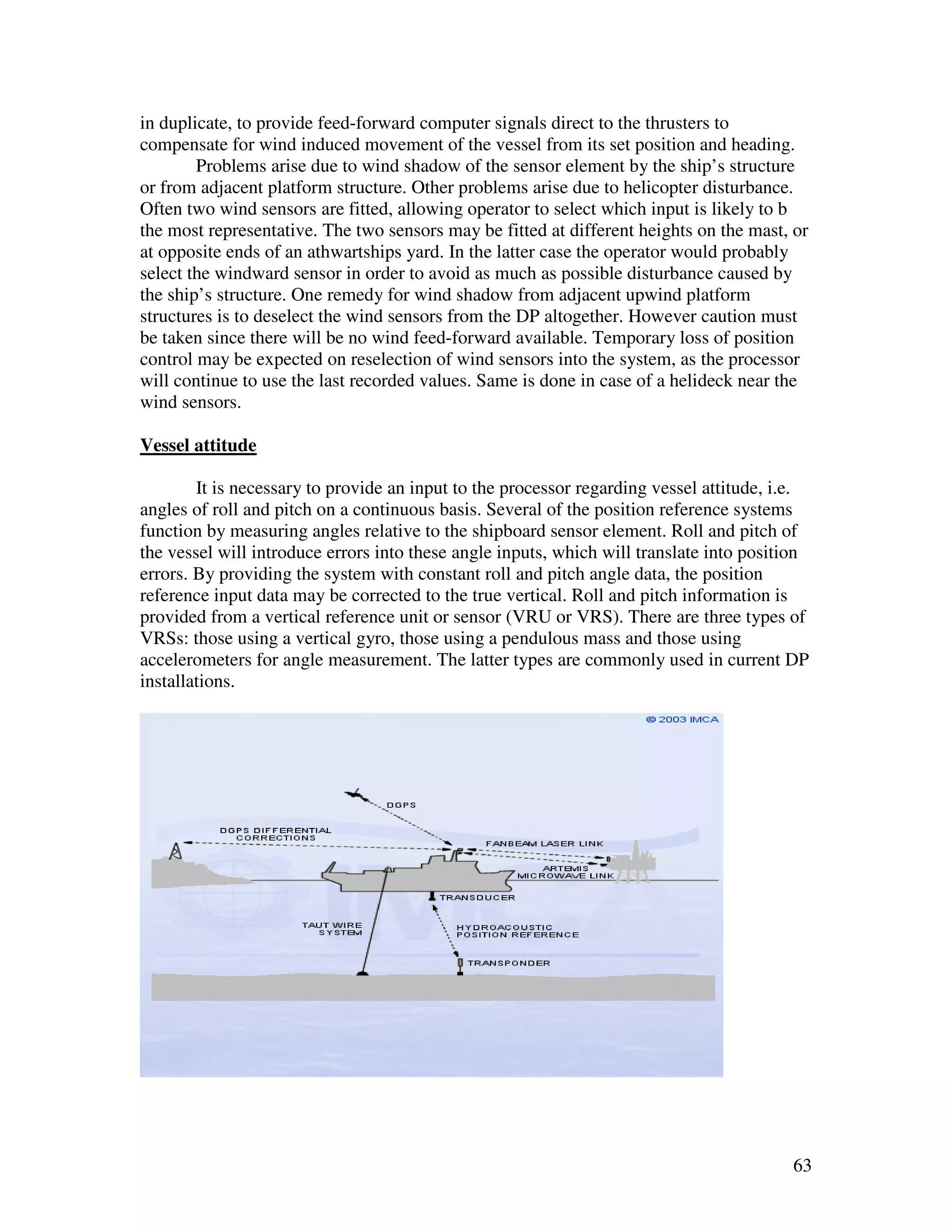
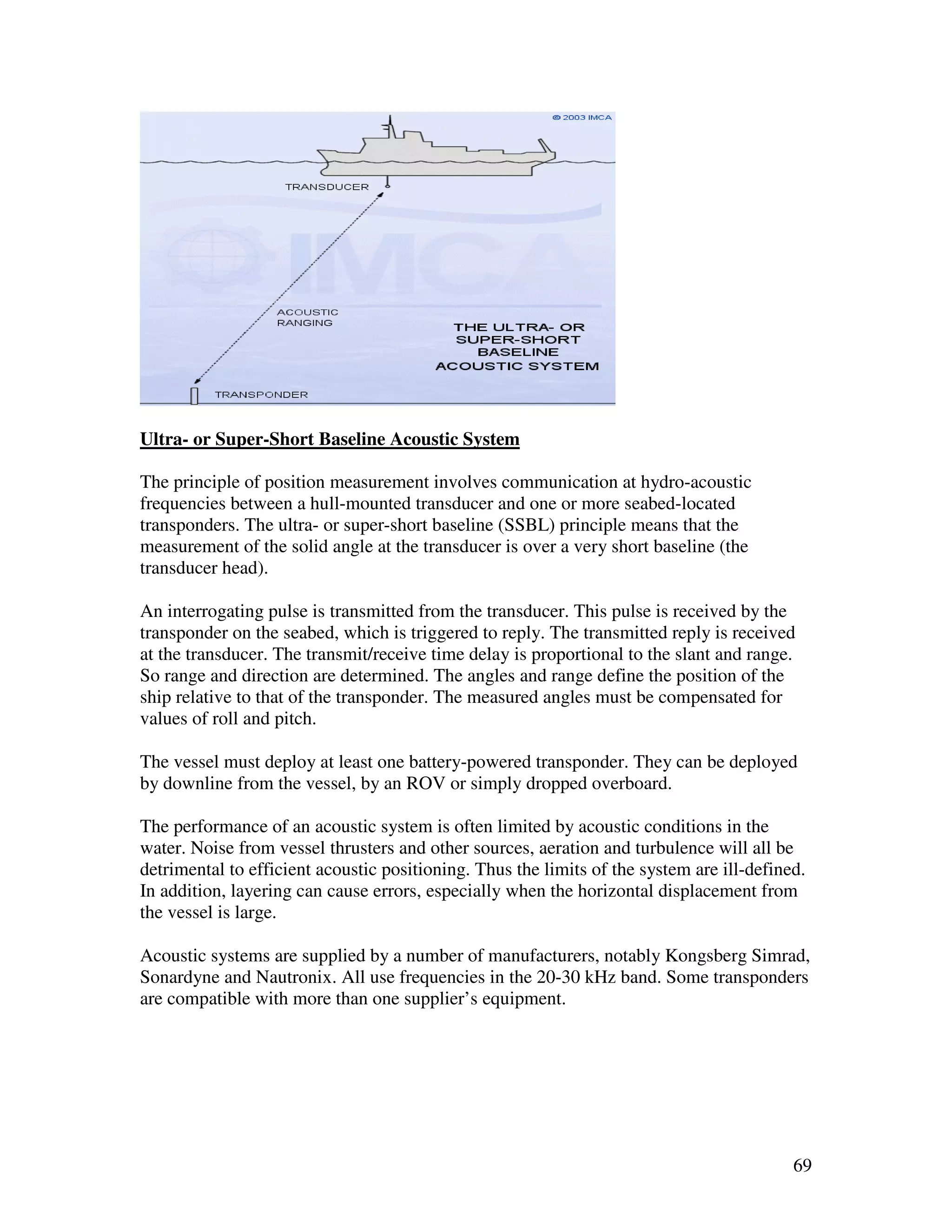
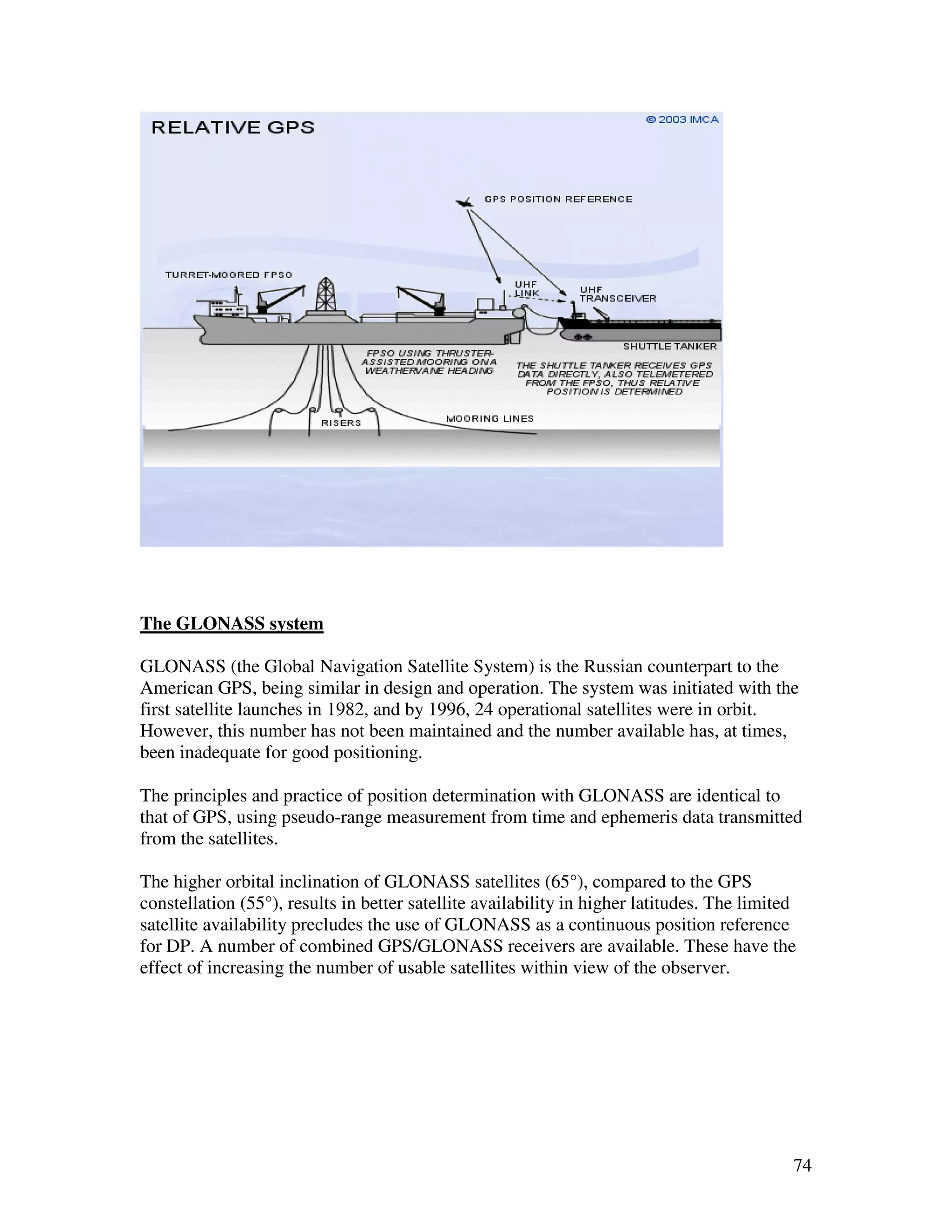
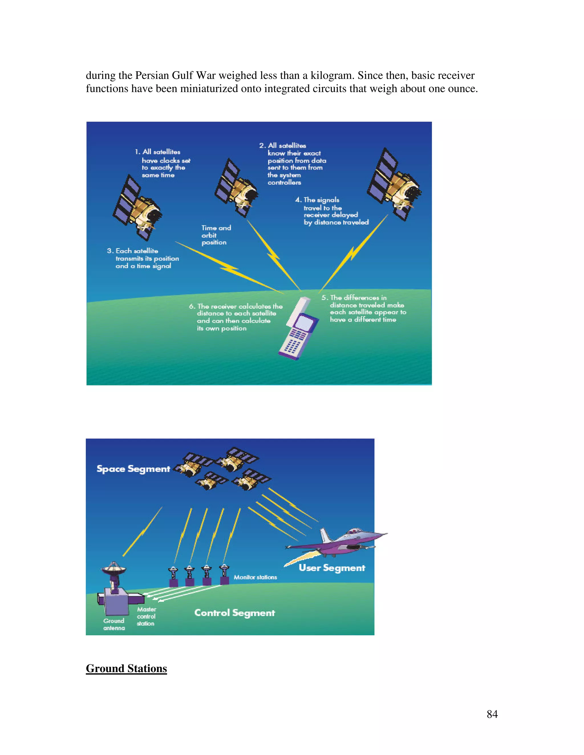
![The main elements of a dynamic positioning system are the position reference system, the
propulsion system and the control system. The position of the vessel can be measured
using either an hydro-acoustic system (beacon), a taut-wire system, a micro-wave radio
system, GPS or a combination of them. The deviation of the vessel heading is measured
by a gyrocompass. The direction and magnitude of wind are measured by a wind sensor
(anemometer). The propulsion system can be composed of various combinations of main
engine, tunnel thrusters, steerable thrusters and cycloidal propellers. The control system
receives signals of the position reference system and heading deviations, compares with
ordered values and calculates the output commands for thrust magnitude and direction of
thrust devices.
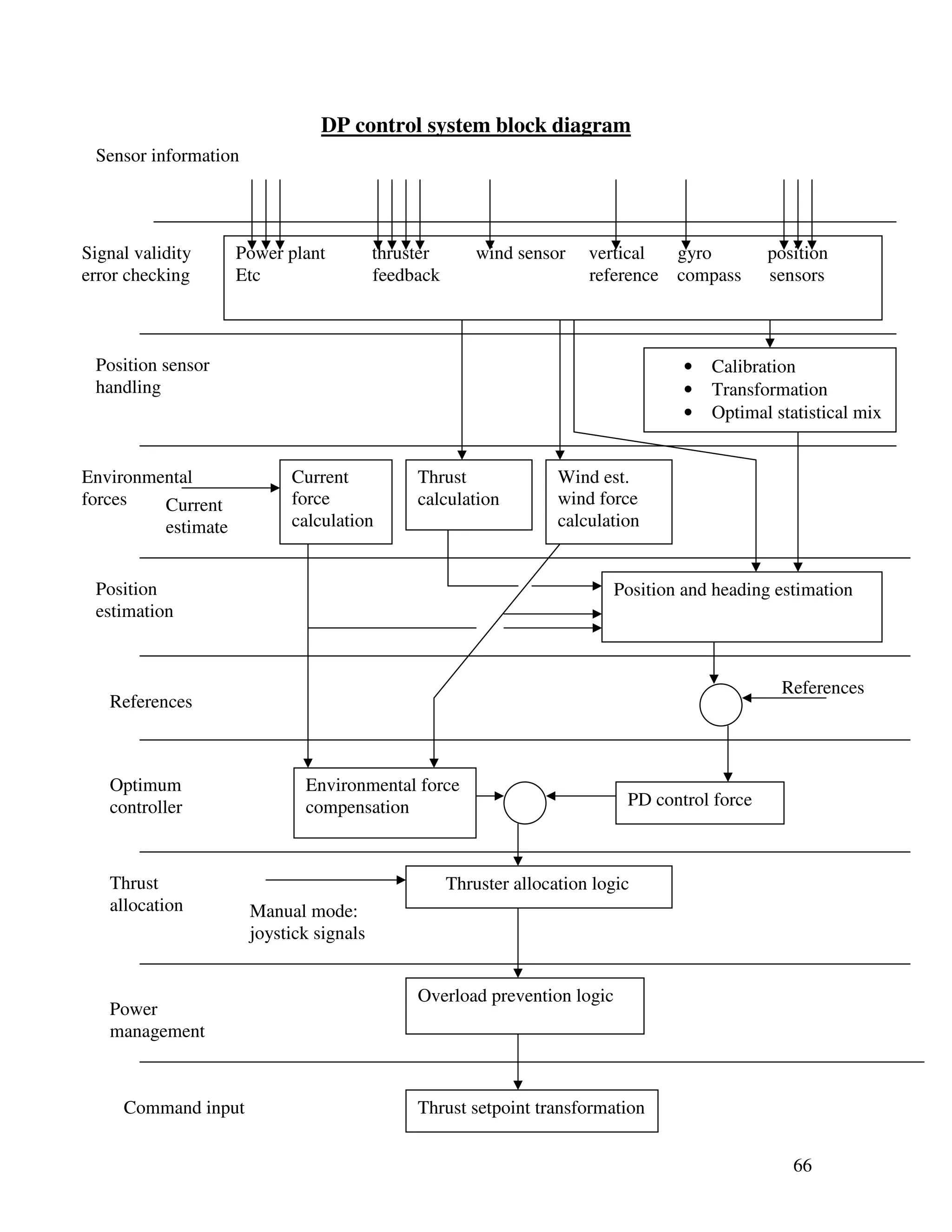
The DP system is an example of closed loop or feedback control using mathematical
modeling. A separate model is required for the dynamic of the vessel hull, the thrusters,
each position reference system, and also the various other sensors used. The ultimate
function of the control system is to compute thruster command that will, when applied to
the thrusters, maintain the vessel on station or return the vessel to the set position and
heading. The optimal control strategy for the dynamic positioning design can be split into
the following distinct procedures, [2]:
• Find the optimal feedback; the use of modeling techniques allows for combination
of several position reference systems in a pooling arrangement; observed position
spreads allow a bias to be calculated to each system so that optimum value for the
ship’s position is continuously calculated.
• The magnitude and direction of the wind are measured, converted to ship
coordinate system, filtered and input into the wind feed-forward loop (feed-
forward problem);
• The thruster allocation algorithm calculates thruster output level and azimuth
angle commands to an arbitrary combination of working propulsion plant
(contribution problem).
One of the most important forces that must be compensated for is that resulting from
wind. Since the wind speed and direction are subject to very rapid changes and since the
vessel is rapidly influenced by wind forces, it is necessary to provide direct thruster
compensation for measured wind variations. This is referred to as feed-forward and
requires an accurate wind sensor input in order to function. Without wind feed-forward,
changes in wind speed and direction would not be compensated for until the model was
fully updated.
POSITION REFERENCE SYSTEMS
Accurate, reliable and continuous position information is essential for dynamic
positioning. Some DP operations require better than 3m relative accuracy. A DP control
system requires data at a rate of once per second to achieve high accuracy. Reliability is,
of course, of vital importance, to operations where life and property may be put at
extreme risk through incorrect position data.
67](https://image.slidesharecdn.com/final1-091028042342-phpapp02/75/Motion-stability-and-control-in-marine-surface-vessels-67-2048.jpg)
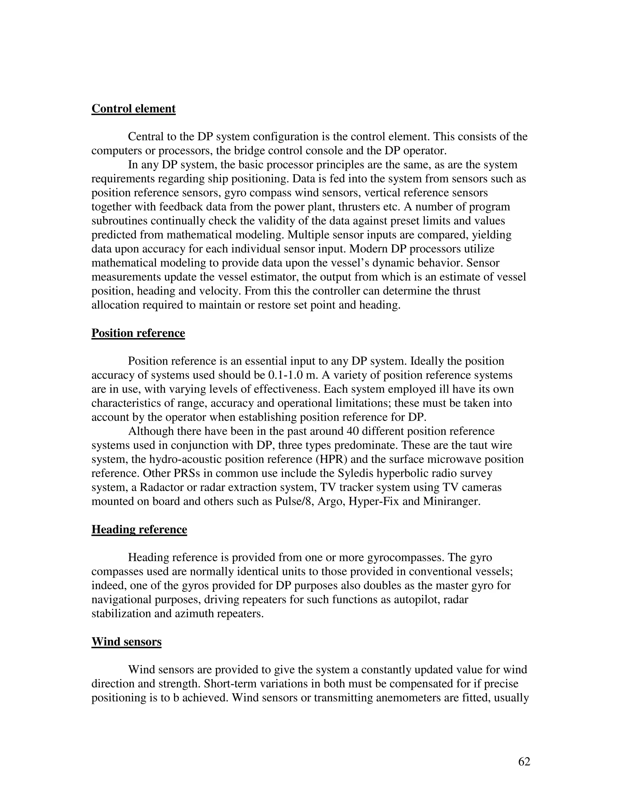
![APPENDIX – A
Code for the ship simulation program for motion stability
N = 6000; % number of samples break
h = 0.1; % sampling time end
w = 0;
% cargo ship if i==1000, w = 1; end % impulse w(t) at time
K = 0.185; T = 107.3; uo = 5.0; t = 100 (s)
No = menu('Choose maneuver','Straight- r = r + h*(-r + K*delta + w)/T; % Euler
line stability',... integration
'Directional stability (critical psi = psi + h*r;
damped)',... x = x + h*uo*cos(psi);
'Directional stability y = y + h*uo*sin(psi);
(underdamped)',... end
'Positional motion stability',...
'Exit'); % plots
if No~=5,
% main loop t = h*(0:N)';
r=0; psi=10; x=0; y=0; delta = 0; z=0; r=(180/pi)*xout(:,1); psi=(180/pi)*xout(:,2);
xout = zeros(N+1,5); x=xout(:,3); y=xout(:,4);
delta=(180/pi)*xout(:,5);
for i=1:N+1,
xout(i,:) = [r psi x y delta]; clf;figure(1),figure(gcf)
subplot(211);plot(x,y,'b','linewidth',2),hold on
if No==1,
delta = 0; plot(x,0*zeros(length(x),1),'r','linewidth',2),hold
elseif (No==2 | No==3), off
if No==2, zeta = 1; wn = 3/T; end grid
if No==3, zeta = .1; wn = 3/T; end if No==1, title('XY-Plot: Straight-line
Kp = (T/K)*wn*wn; % PD- stability');
control elseif No==2, title('XY-Plot: Directional
Kd = (T/K)*(2*zeta*wn+1/T); stability (critical damped)');
delta = -Kp*(psi)-Kd*r; elseif No==3, title('XY-Plot: Directional
elseif No==4, stability (underdamped)');
zeta = 1; wn = 7/T; elseif No==4, title('XY-Plot: Positional motion
Kp = (T/K)*wn*wn; stability');
Kd = (T/K)*(2*zeta*wn+1/T); end
Ki = Kp*wn/10; subplot(223);plot(t,r,'linewidth',2),grid,title('r
delta = -Kp*(psi)-Kd*r-Ki*z; % (deg/s)'),xlabel('sec')
PID-control
z = z + h*psi; subplot(224);plot(t,psi,'linewidth',2),grid,title('psi
else (deg)'),xlabel('sec')
stabdemo
else
close all
end
81](https://image.slidesharecdn.com/final1-091028042342-phpapp02/75/Motion-stability-and-control-in-marine-surface-vessels-81-2048.jpg)

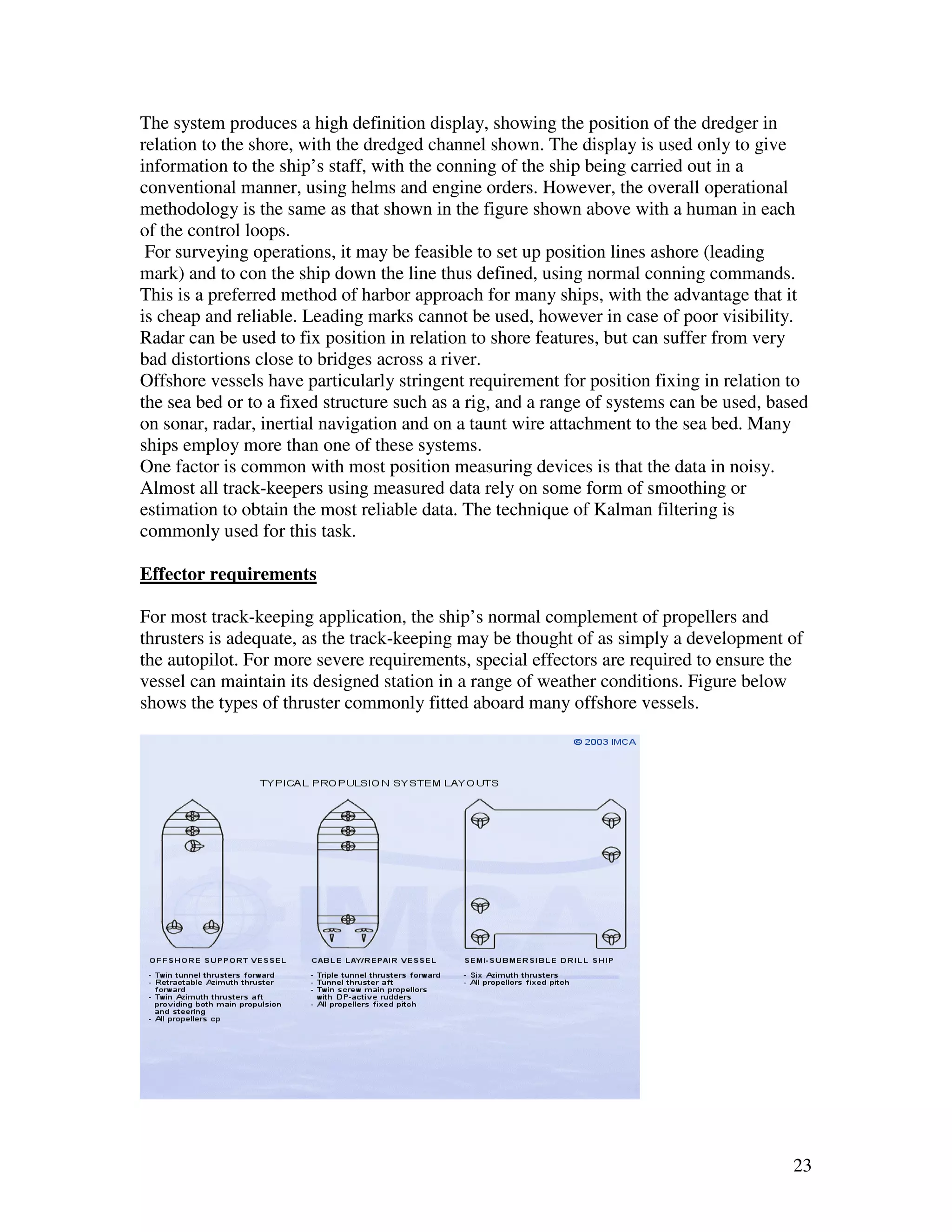
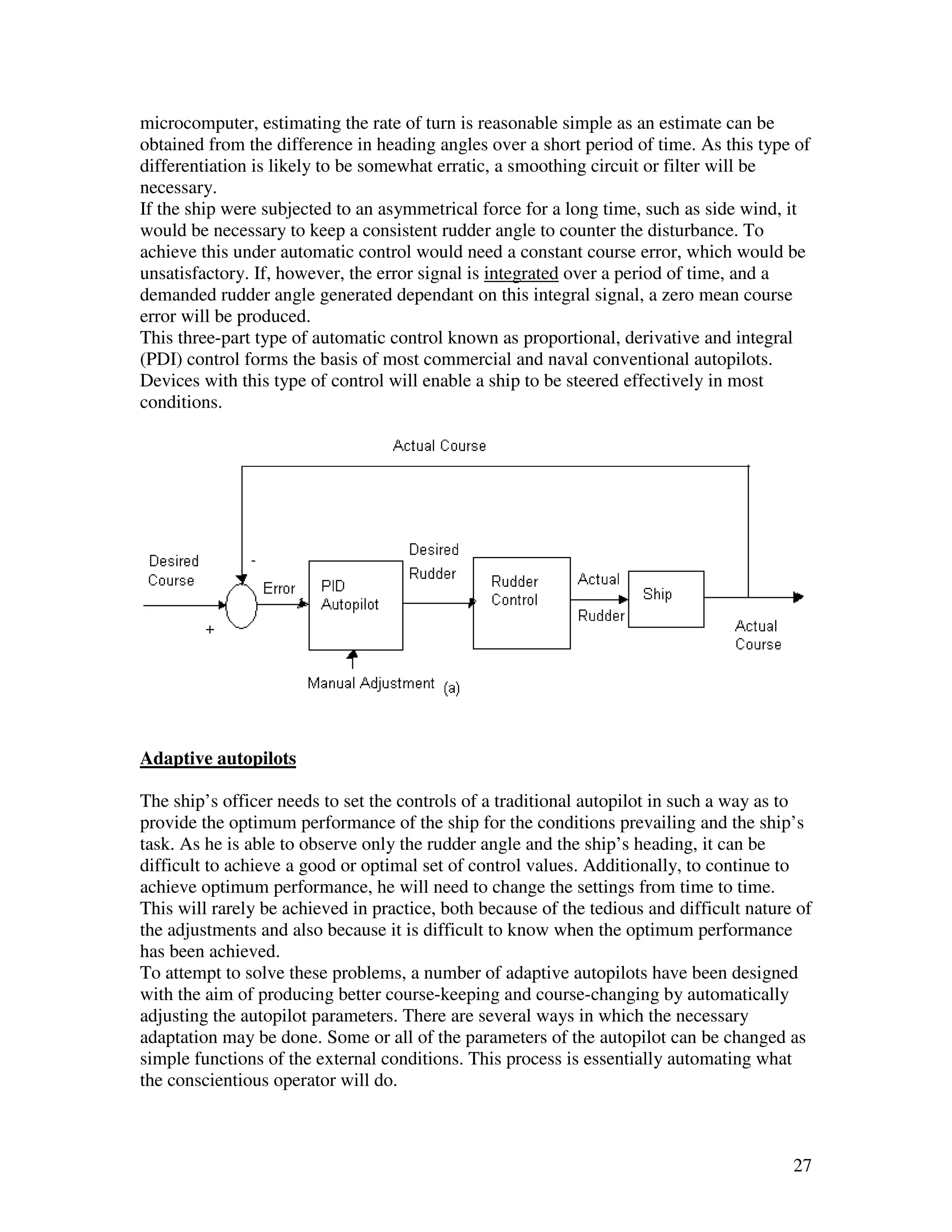
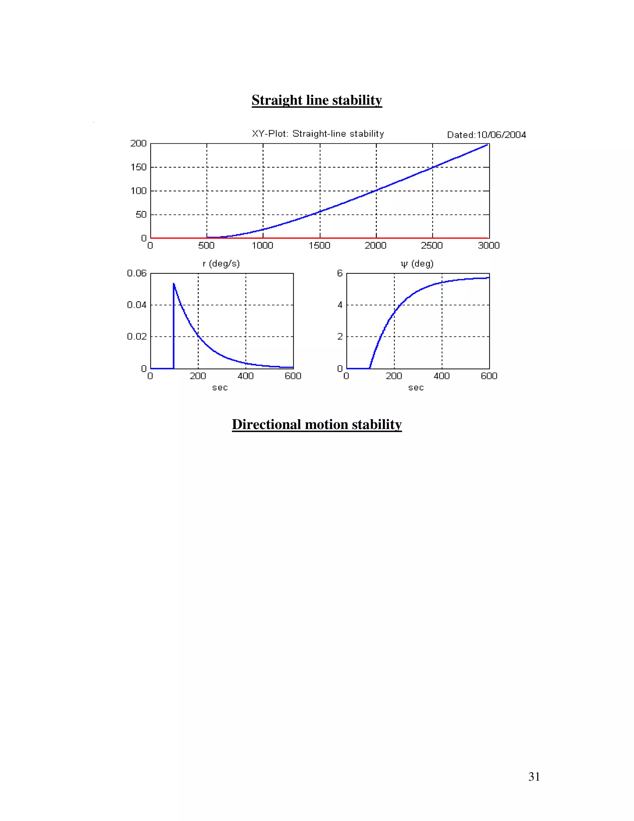
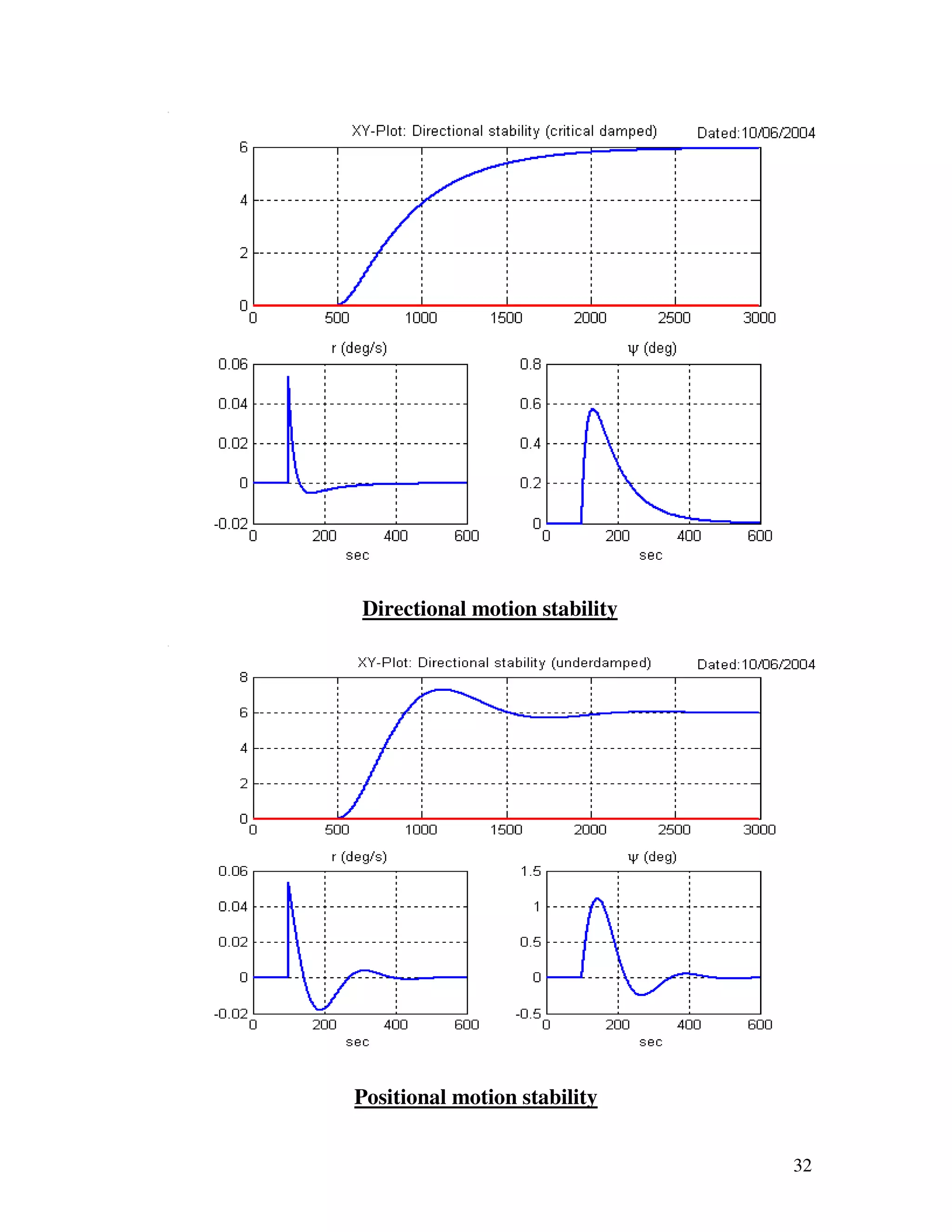
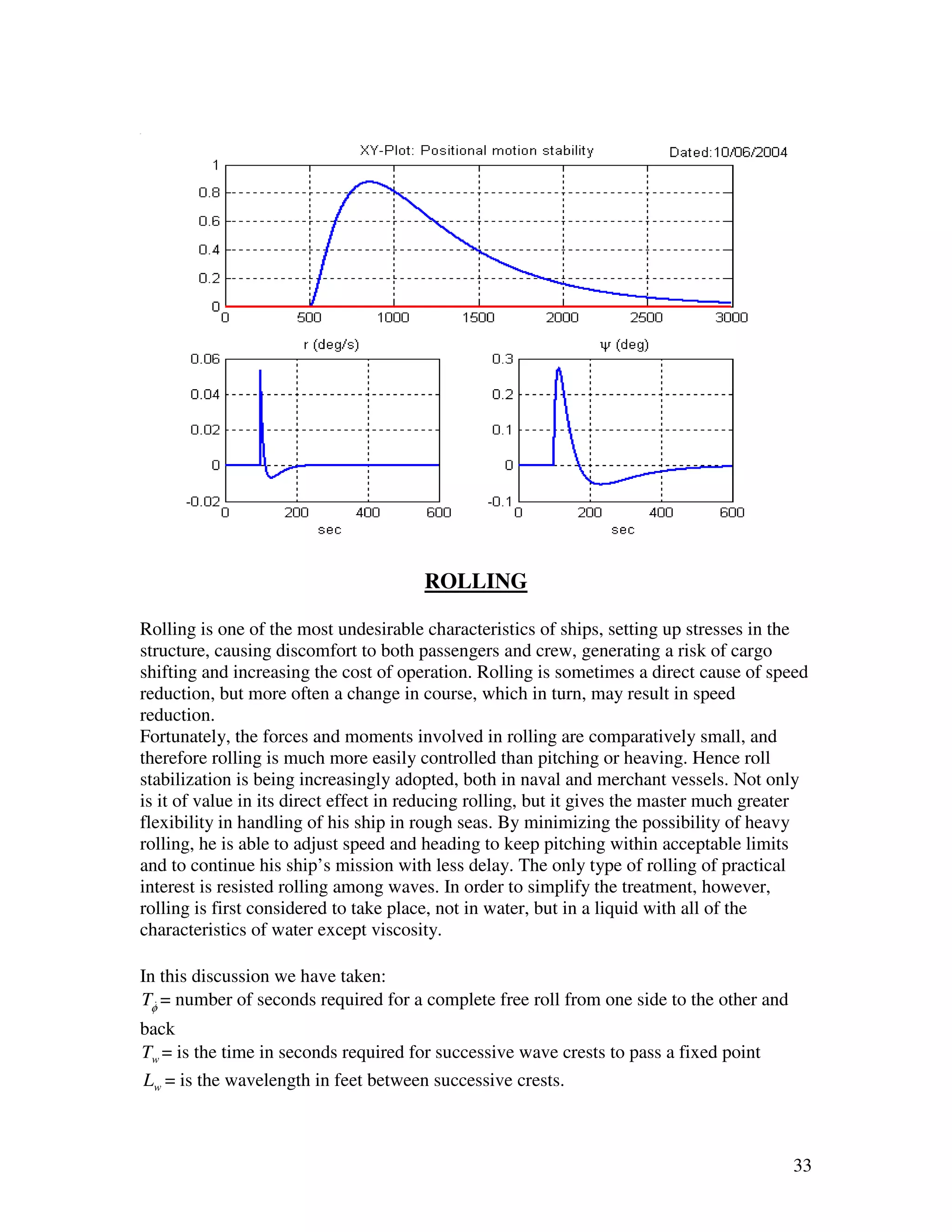
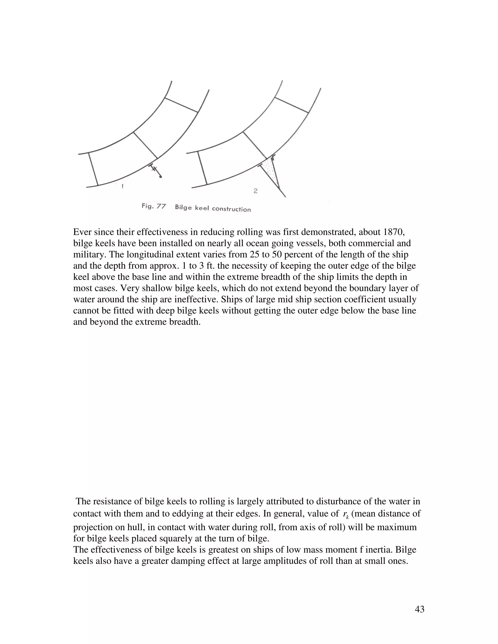
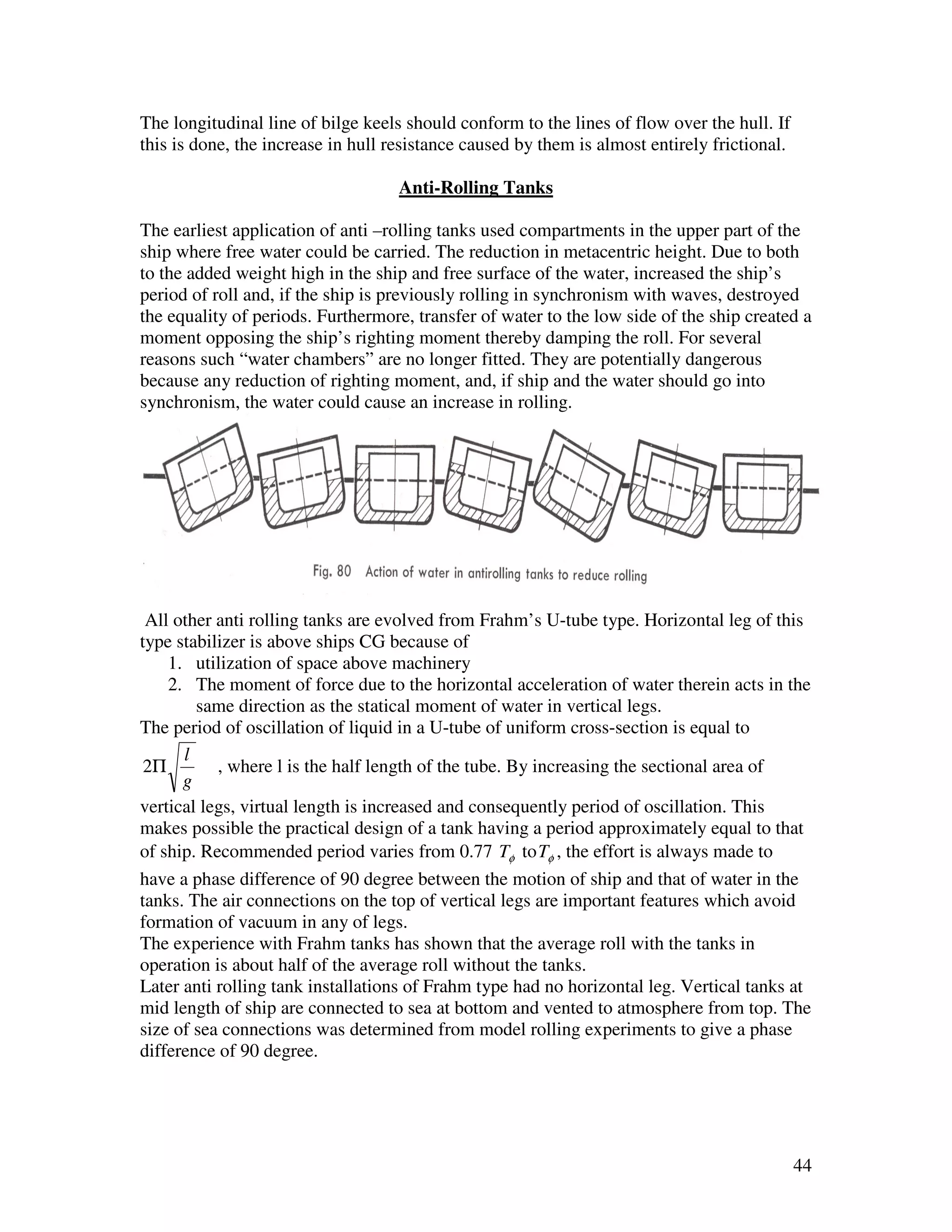
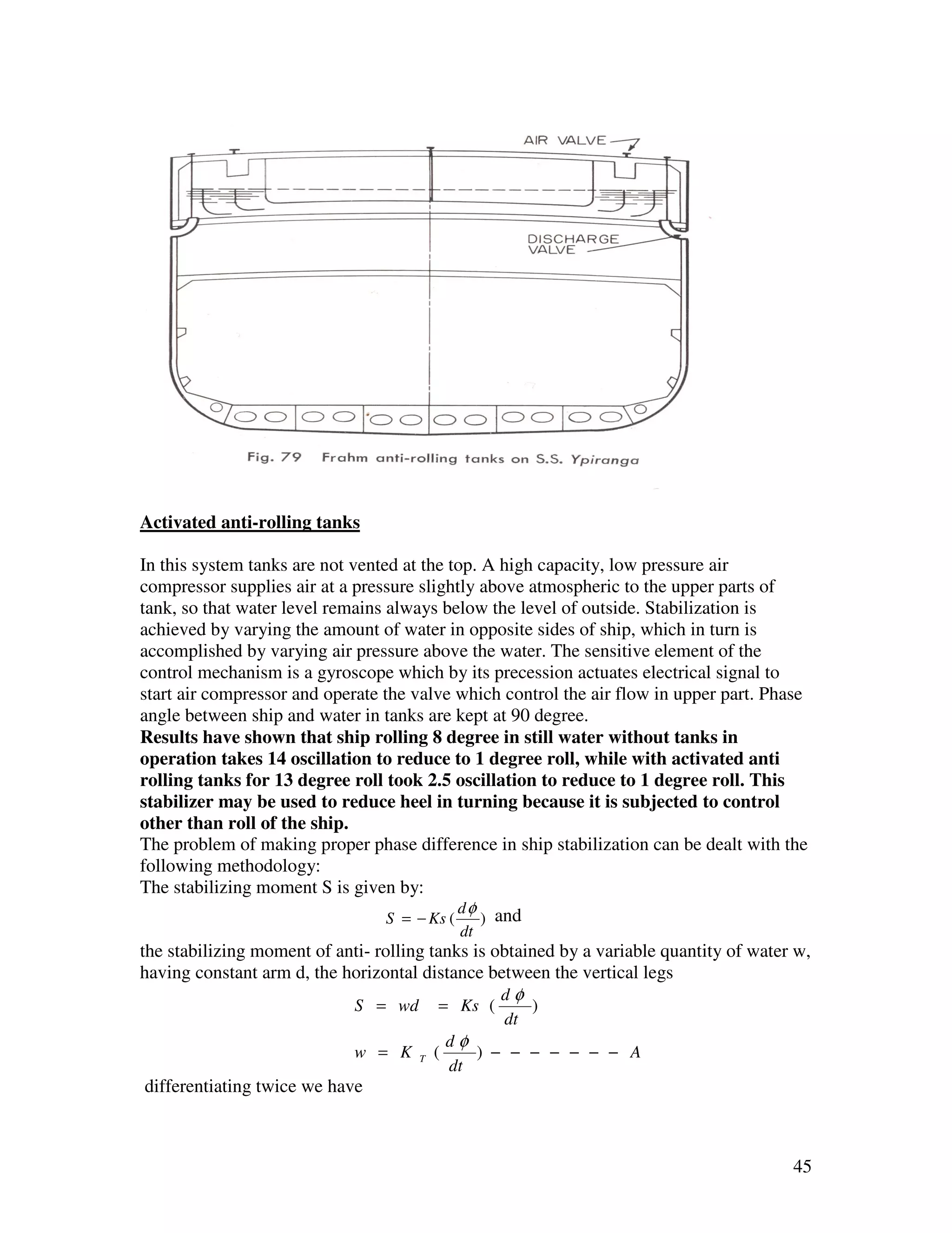
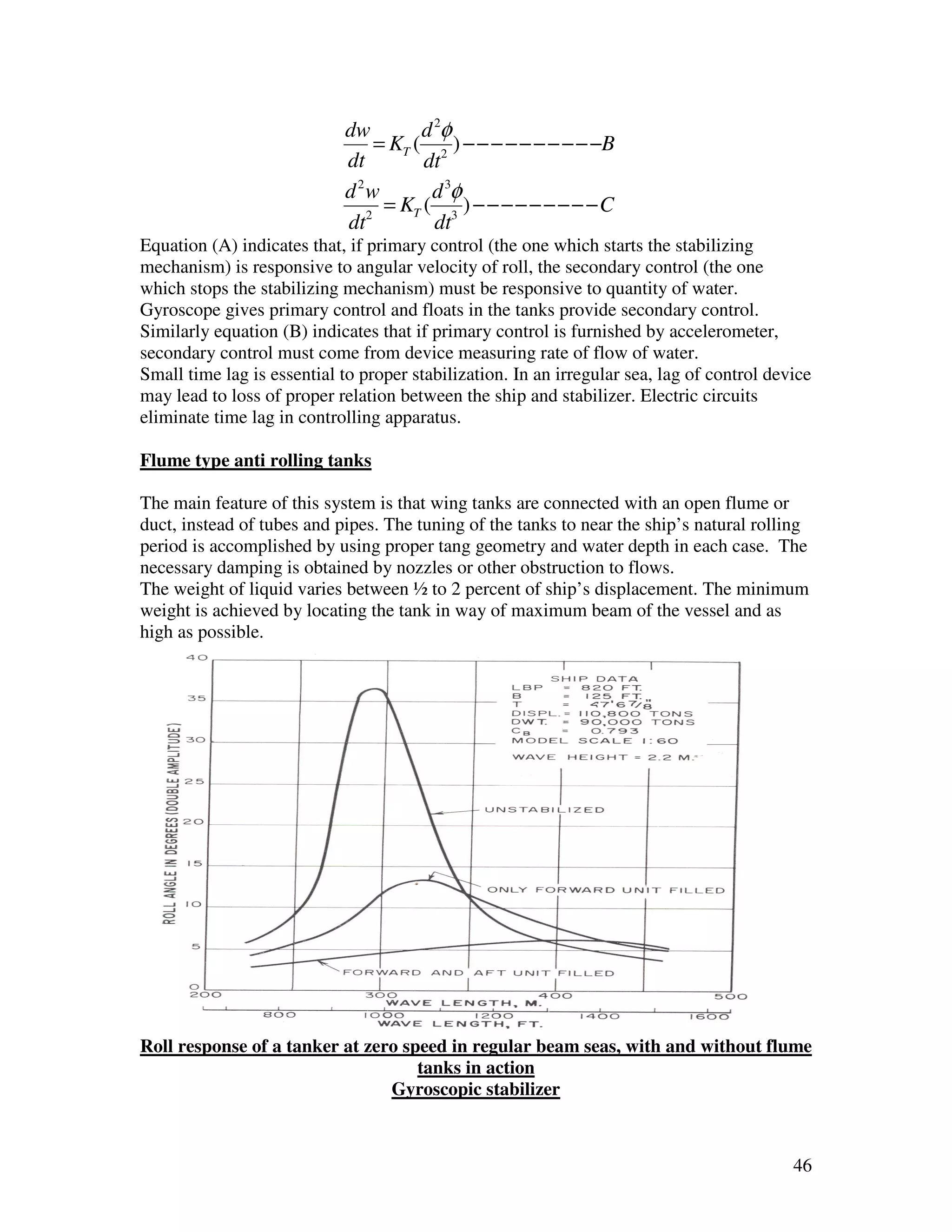
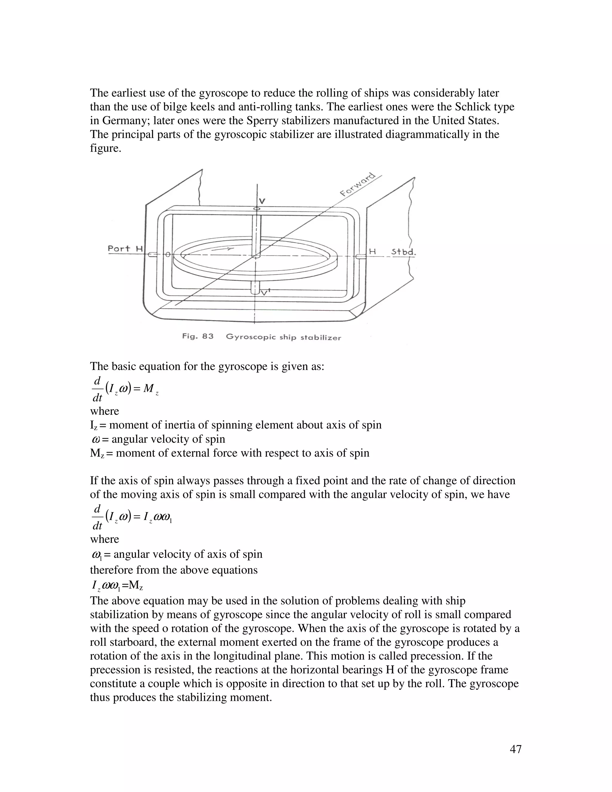
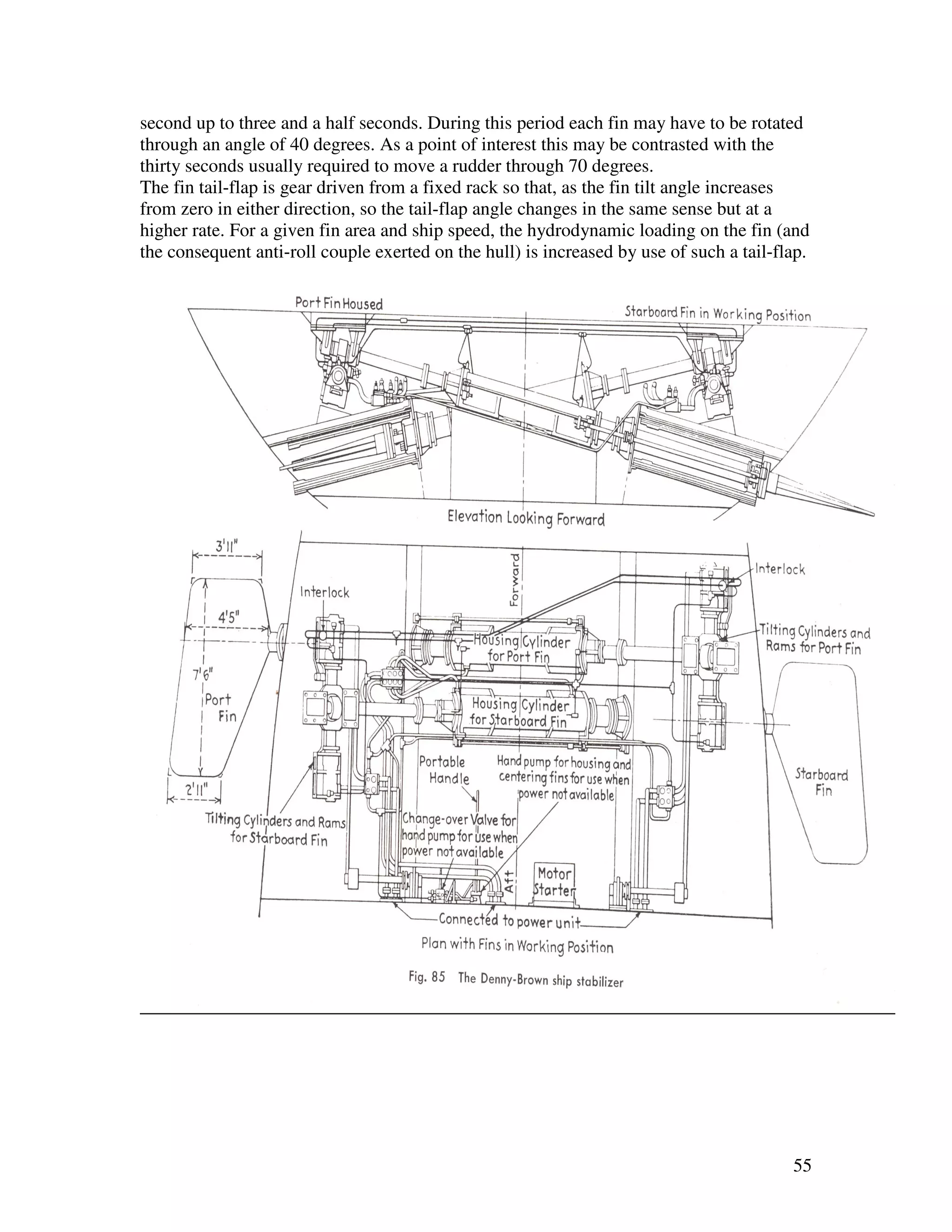
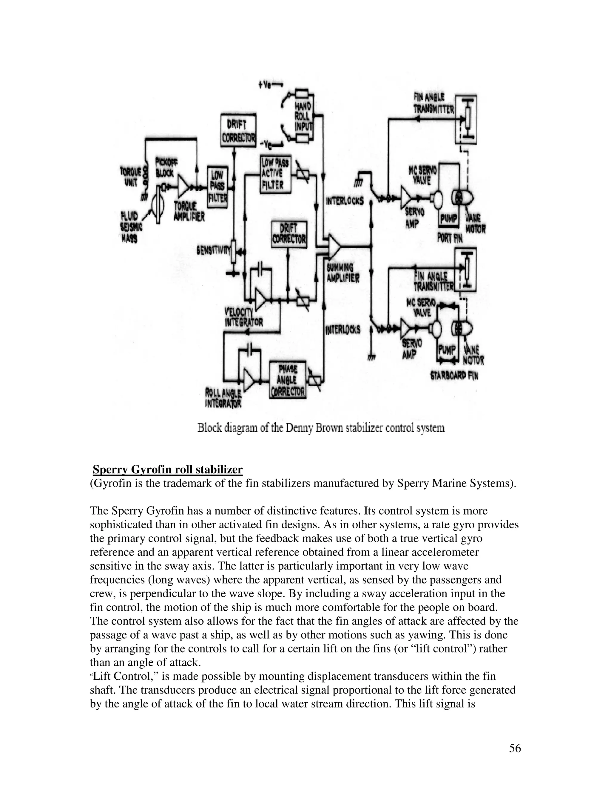
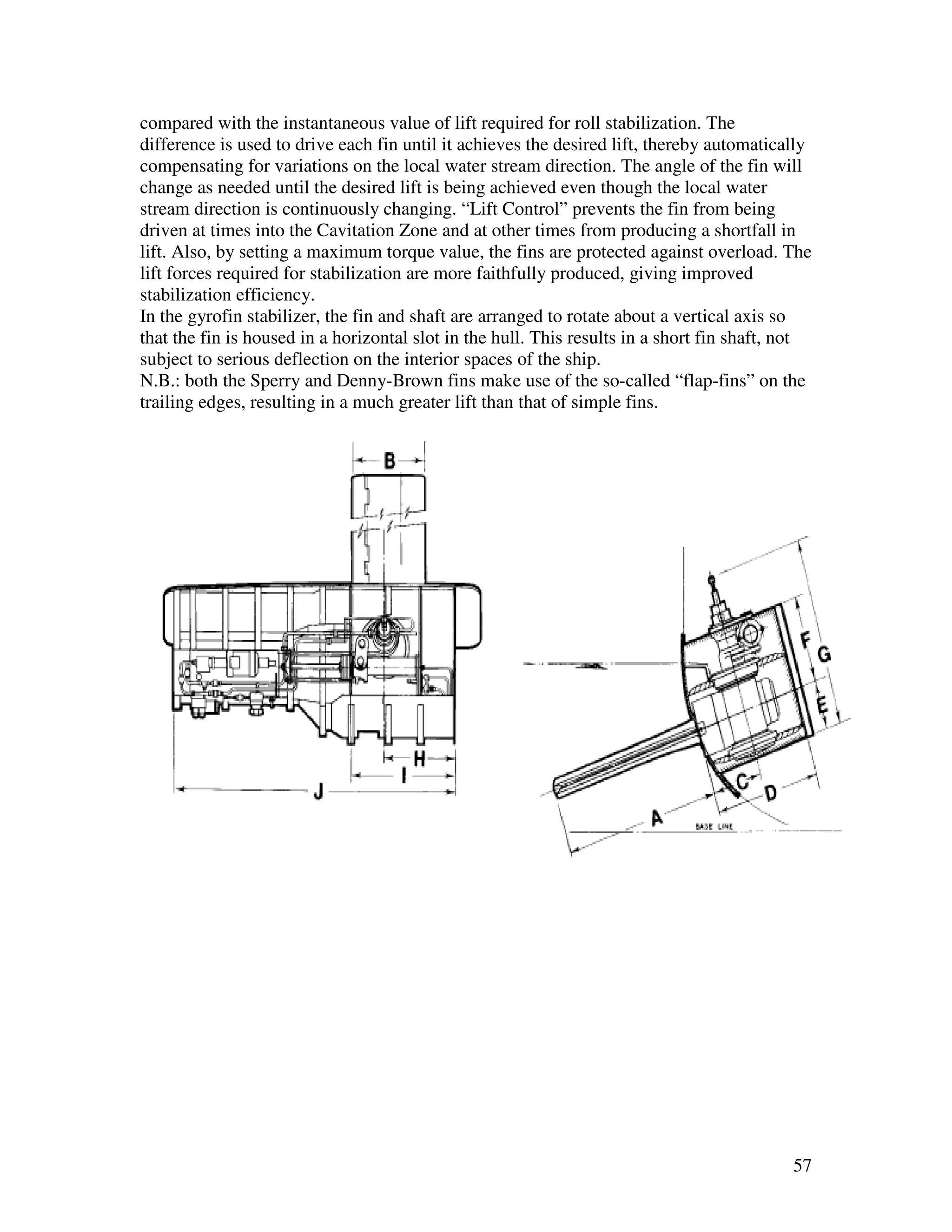
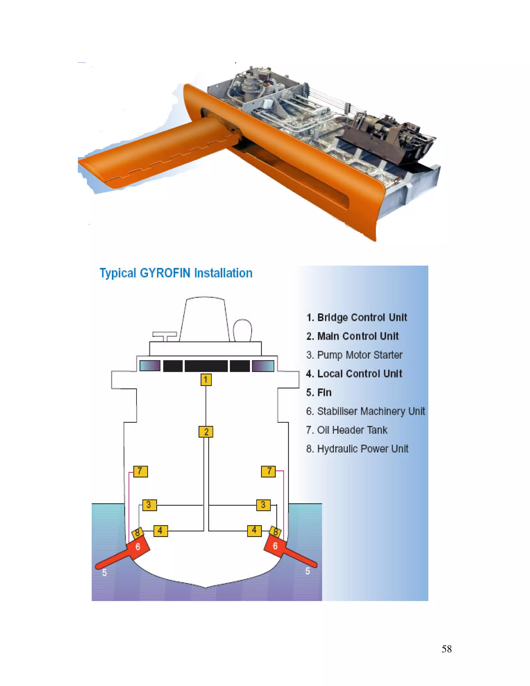
This document discusses principles of motion stability and control for marine surface vessels. It covers topics like heading control, track keeping, dynamic positioning, and roll stabilization. Mathematical modeling is used to analyze ship motions and develop control systems, with newer algorithms discussed theoretically. Simulation software is also utilized to obtain results on motion stability and control codes.


![[2] ship classification and types](https://cdn.slidesharecdn.com/ss_thumbnails/2shipclassificationandtypes-120403042444-phpapp01-thumbnail.jpg?width=640&height=640&fit=bounds)


