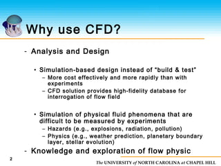
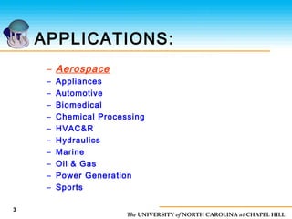
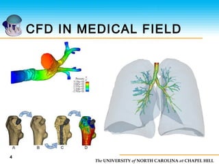
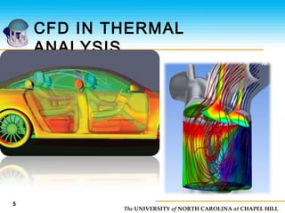
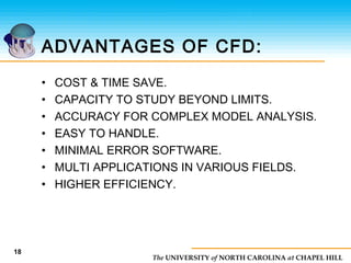
This document discusses computational fluid dynamics (CFD) and its applications. It provides an overview of why CFD is used for analysis and design, specifically for simulating fluid phenomena more cost effectively and rapidly than physical experiments. It also lists common applications of CFD in fields like aerospace, automotive, biomedical, and more. Additionally, it outlines the basic steps of CFD which include dividing the fluid volume into sections, simplifying equations, setting boundary conditions, and solving the equations to model fluid flow.

1. The UNIVERSITY of NORTH CAROLINA at CHAPEL HILL
Computational Fluid
Dynamics
MOHAN REDDY GADE
11D41A0382
MECHANICAL-B
B-tECH fINAL YEAR

2. The UNIVERSITY of NORTH CAROLINA at CHAPEL HILL
Why use CFD?
- Analysis and Design
• Simulation-based design instead of “build & test”
– More cost effectively and more rapidly than with
experiments
– CFD solution provides high-fidelity database for
interrogation of flow field
• Simulation of physical fluid phenomena that are
difficult to be measured by experiments
– Hazards (e.g., explosions, radiation, pollution)
– Physics (e.g., weather prediction, planetary boundary
layer, stellar evolution)
- Knowledge and exploration of flow physic
2

3. The UNIVERSITY of NORTH CAROLINA at CHAPEL HILL
APPLICATIONS:
– Aerospace
– Appliances
– Automotive
– Biomedical
– Chemical Processing
– HVAC&R
– Hydraulics
– Marine
– Oil & Gas
– Power Generation
– Sports
3

4. The UNIVERSITY of NORTH CAROLINA at CHAPEL HILL
CFD IN MEDICAL FIELD
4

5. The UNIVERSITY of NORTH CAROLINA at CHAPEL HILL
CFD IN THERMAL
ANALYSIS
5

6. The UNIVERSITY of NORTH CAROLINA at CHAPEL HILL
6

7. The UNIVERSITY of NORTH CAROLINA at CHAPEL HILL
7

8. The UNIVERSITY of NORTH CAROLINA at CHAPEL HILL
Steps to CFD
1. Divide the fluid volume (surface) up
into manageable chunks (gridding).
2. Simplify the equations to be solved
3. Set boundary conditions.
4. Initialise the other grid values.
5. Step through the grid ensuring that
these simplified equations are
satisfied at the grid points and nearest
neighbours.
8

9. The UNIVERSITY of NORTH CAROLINA at CHAPEL HILL
How does a CFD code
work?
• Preprocessor
- create geometry
- mesh volume
• Processor
- solve a system of equations
- approximation to subset or superset of
Navier-Stokes equations
• Post-processor
- Vector plots, contour plots, integrated
values (eg total pressure)
- Colour For Directors
9

10. The UNIVERSITY of NORTH CAROLINA at CHAPEL HILL
10
Overview
• Understanding the Navier-Stokes
equations
- Derivation (following [Griebel 1998])
- Intuition
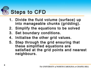
• Solving the Navier-Stokes equations
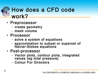
- Basic approaches
- Boundary conditions
• Tracking the free surface

11. The UNIVERSITY of NORTH CAROLINA at CHAPEL HILL
11
Transport Theorem
xdtxuff
t
xdtxf
dt
d
t t

),()div(),(∫ ∫Ω Ω






+
∂
∂
=
),(),( tc
t
txu

Φ
∂
∂
=),( tcx

Φ=
c

0Ω
),( tc

Φ
tΩ

12. The UNIVERSITY of NORTH CAROLINA at CHAPEL HILL
12
Conservation of Mass
densityis;),()0,(mass
0
ρρρ ∫∫ ΩΩ
==
t
xdtxxdx

0),()div(),( =






+
∂
∂
=∫ ∫Ω Ω
xdtxu
t
xdtx
dt
d
t t

ρρρ
0)div( =+
∂
∂
u
t

ρρ
Transport theorem
0div =u

Integrand vanishes
ρ is constant
for incompressible
fluids
Continuity equation

13. The UNIVERSITY of NORTH CAROLINA at CHAPEL HILL
13
Conservation of
Momentum
∫Ω
=
t
xdtxutx

),(),(momentum ρ
∑= forcesactingmomentuminchange
∫Ωt
xdtxftx

),(),(:forcesbody ρ
∫Ω∂ t
dsntx

),(:forcessurface σ
∫∫∫ Ω∂ΩΩ
+=
ttt
dsntxxdtxftxxdtxutx
dt
d 
),(),(),(),(),( σρρ
normal:tensorstress: n

σ

14. The UNIVERSITY of NORTH CAROLINA at CHAPEL HILL
14
Conservation of
Momentum
0divdiv)())(()( =−−+∇⋅+ σguuuuu
dt
d 
ρρρρ
Transport theorem Divergence
theorem
fupuu
dt
ud 

+∇+∇−∇⋅−= 21
)( ν
ρ
Momentum equation
…
∫∫∫ Ω∂ΩΩ
+=
ttt
dsntxxdtxftxxdtxutx
dt
d 
),(),(),(),(),( σρρ

15. The UNIVERSITY of NORTH CAROLINA at CHAPEL HILL
15
Navier-Stokes Equations
fupuu
dt
ud
u



+∇+∇−∇⋅−=
=⋅∇
21
)(
0
ν
ρ
convection viscosity
external
forces
pressure

16. The UNIVERSITY of NORTH CAROLINA at CHAPEL HILL
16
Solving the equations
Basic Approach
1. Create a tentative velocity field.
a. Finite differences
b. Semi-Lagrangian method (Stable Fluids [Stam
1999])
2. Ensure that the velocity field is
divergence free:
a. Adjust pressure and update velocities
b. Projection method

17. The UNIVERSITY of NORTH CAROLINA at CHAPEL HILL
17
Particle Level Set Method
Extrapolated velocities at the surface give
more realistic motion.

18. The UNIVERSITY of NORTH CAROLINA at CHAPEL HILL
ADVANTAGES OF CFD:
• COST & TIME SAVE.
• CAPACITY TO STUDY BEYOND LIMITS.
• ACCURACY FOR COMPLEX MODEL ANALYSIS.
• EASY TO HANDLE.
• MINIMAL ERROR SOFTWARE.
• MULTI APPLICATIONS IN VARIOUS FIELDS.
• HIGHER EFFICIENCY.
18

19. The UNIVERSITY of NORTH CAROLINA at CHAPEL HILL
LIMITATIONS OF CFD
• DIFFICULT TO HANDLE
TURBULENCE FLOW.
• DECREASE ABILITY TO
UNDERSTAND PROBLEM .
• TOO TECHNOLOGICAL
RELIABILITY.
19

20. The UNIVERSITY of NORTH CAROLINA at CHAPEL HILL
20