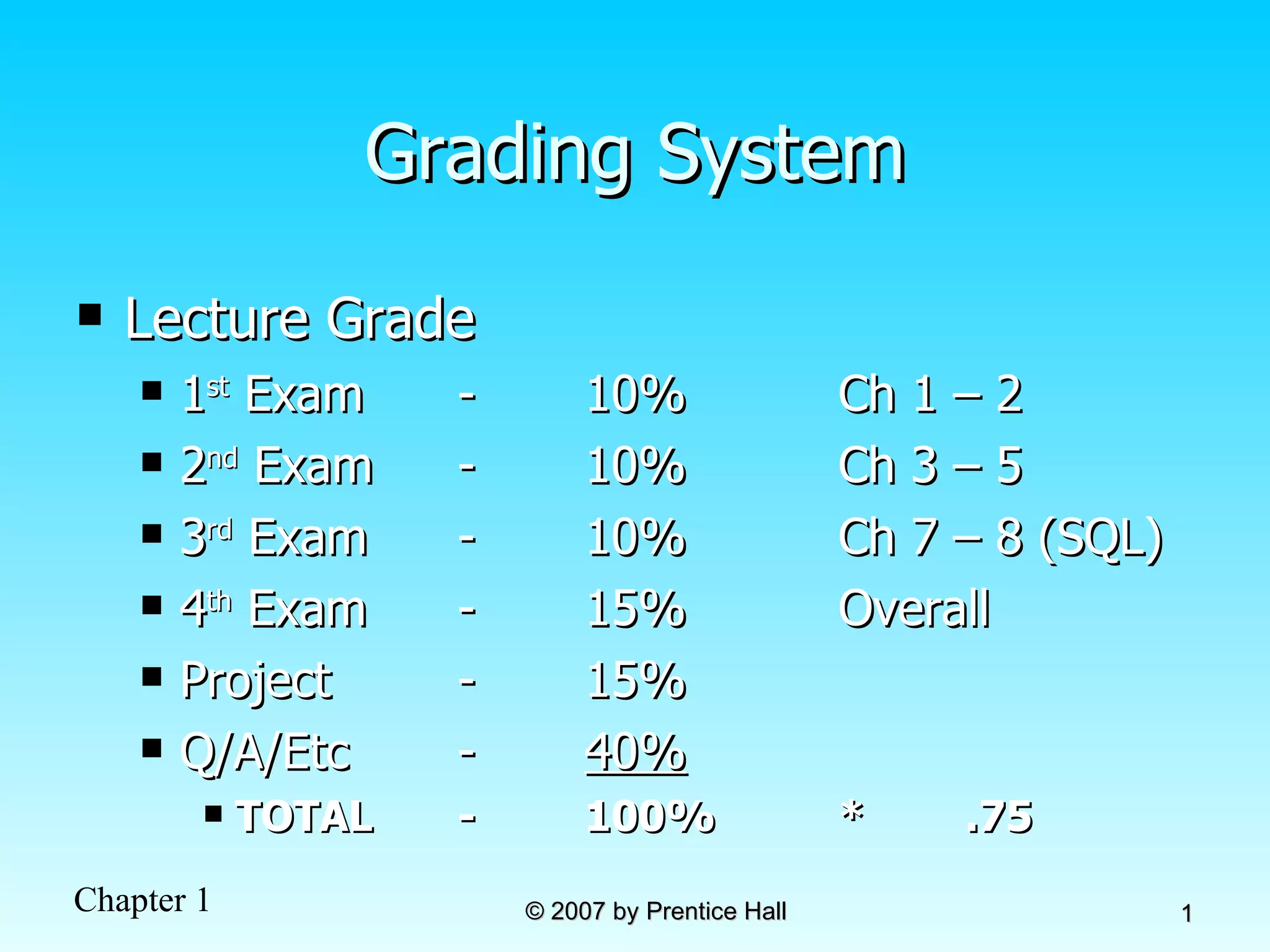
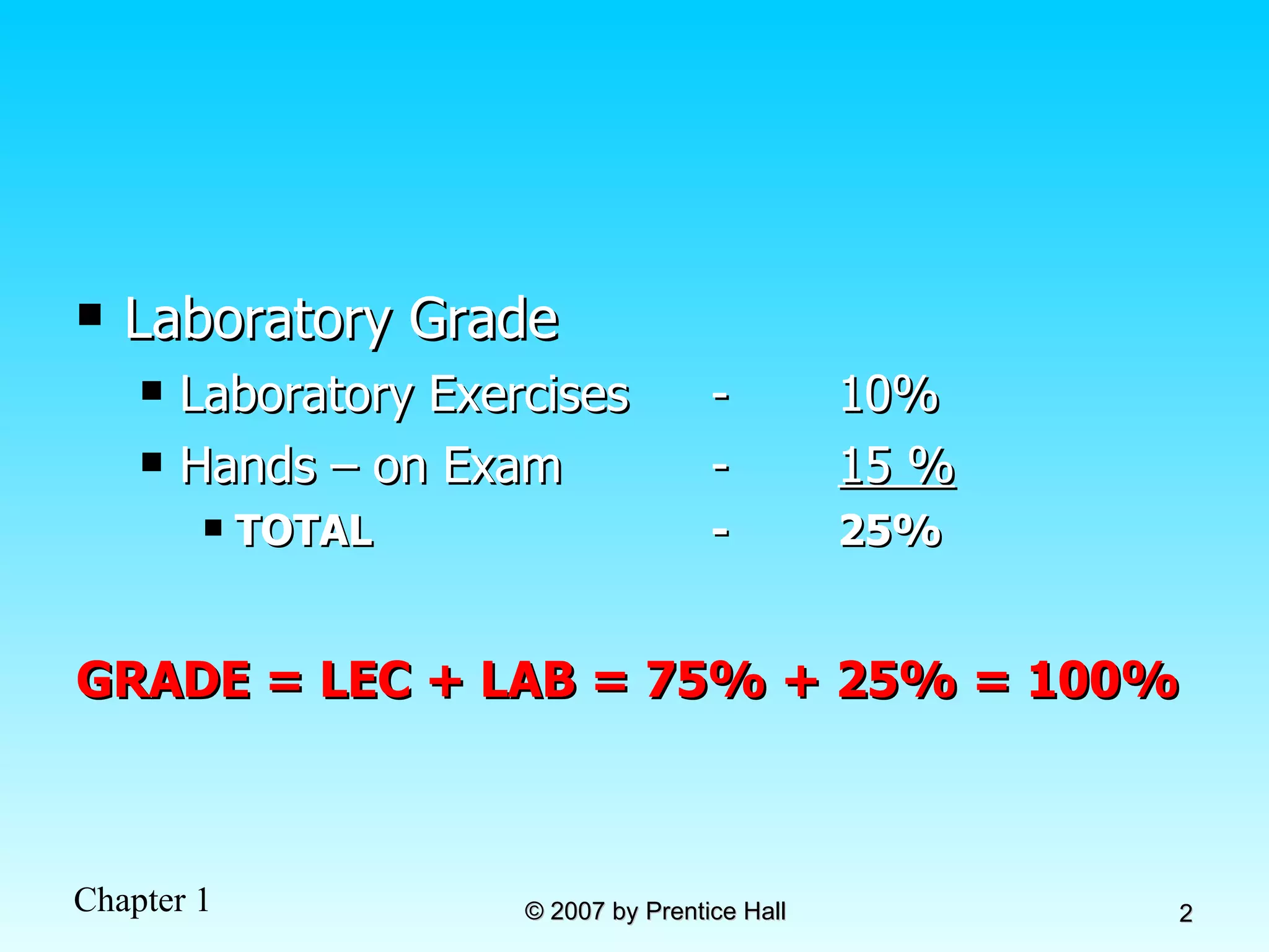
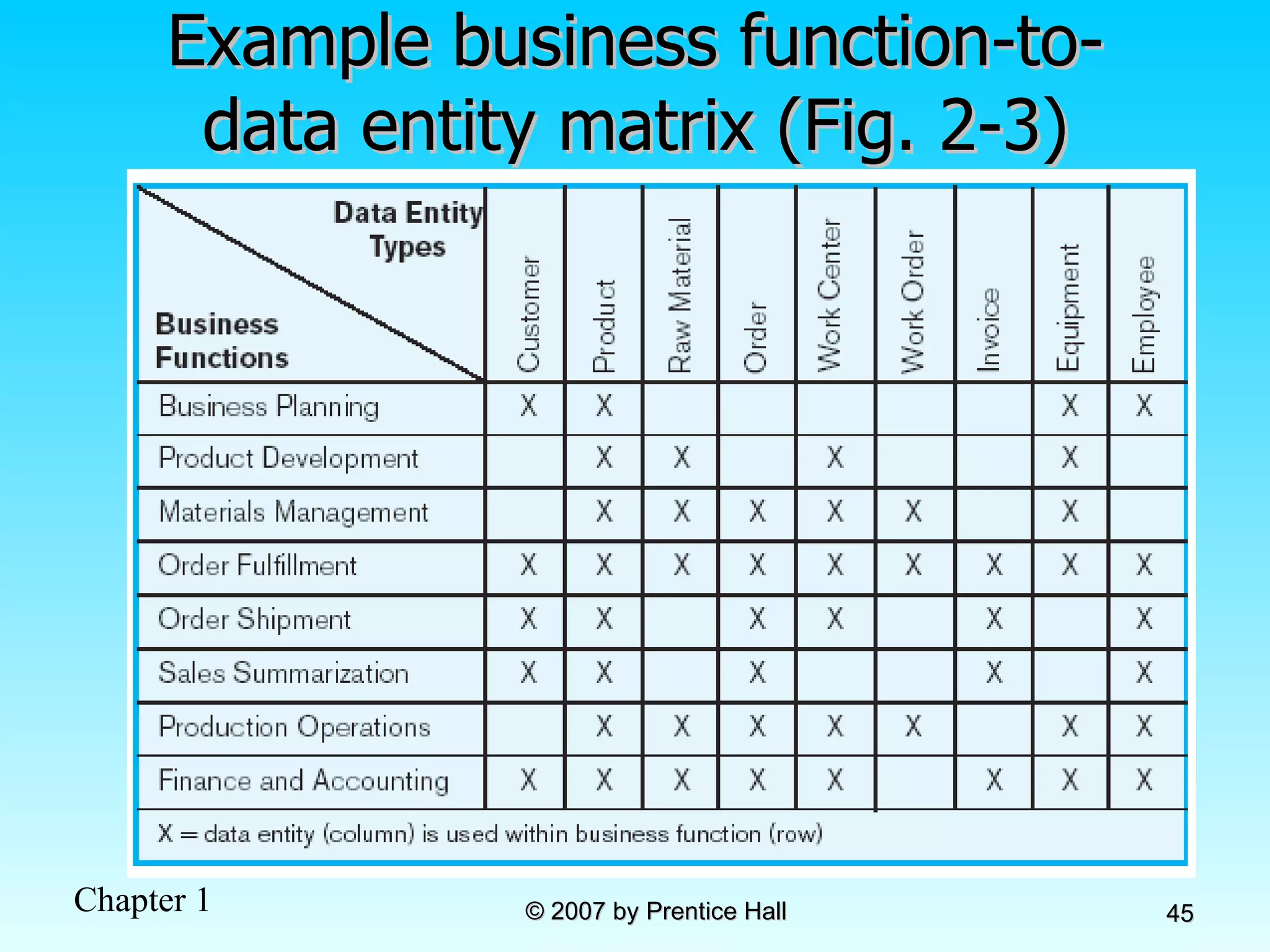
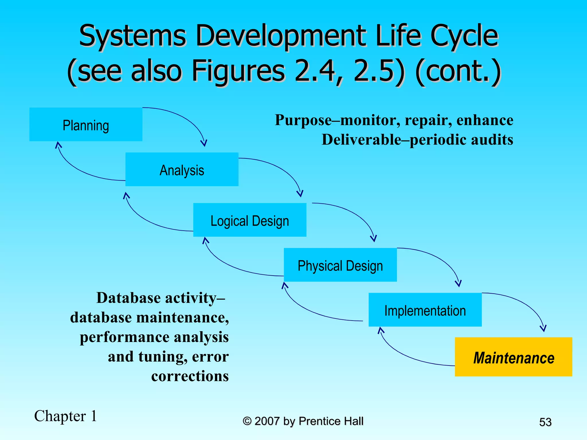
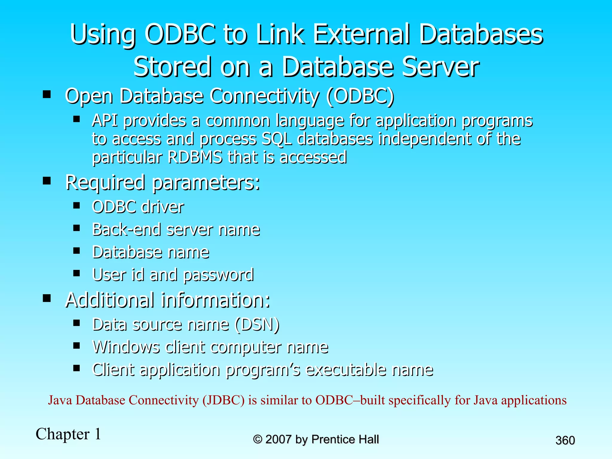
Modern database management jeffrey a. hoffer, mary b. prescott,

Grading System Lecture Grade 1 st Exam - 10% Ch 1 – 2 2 nd Exam - 10% Ch 3 – 5 3 rd Exam - 10% Ch 7 – 8 (SQL) 4 th Exam - 15% Overall Project - 15% Q/A/Etc - 40% TOTAL - 100% * .75

Laboratory Grade Laboratory Exercises - 10% Hands – on Exam - 15 % TOTAL - 25% GRADE = LEC + LAB = 75% + 25% = 100%

Objectives Definition of terms Explain growth and importance of databases Name limitations of conventional file processing Identify five categories of databases Explain advantages of databases Identify costs and risks of databases List components of database environment Describe evolution of database systems

Definitions Database: organized collection of logically related data Data: stored representations of meaningful objects and events Structured: numbers, text, dates Unstructured: images, video, documents Information: data processed to increase knowledge in the person using the data Metadata: data that describes the properties and context of user data

Figure 1-1a Data in context Context helps users understand data

Graphical displays turn data into useful information that managers can use for decision making and interpretation Figure 1-1b Summarized data

Descriptions of the properties or characteristics of the data, including data types, field sizes, allowable values, and data context

Disadvantages of File Processing Program-Data Dependence All programs maintain metadata for each file they use Duplication of Data Different systems/programs have separate copies of the same data Limited Data Sharing No centralized control of data Lengthy Development Times Programmers must design their own file formats Excessive Program Maintenance 80% of information systems budget

Problems with Data Dependency Each application programmer must maintain his/her own data Each application program needs to include code for the metadata of each file Each application program must have its own processing routines for reading, inserting, updating, and deleting data Lack of coordination and central control Non-standard file formats

Figure 1-3 Old file processing systems at Pine Valley Furniture Company Duplicate Data

Problems with Data Redundancy Waste of space to have duplicate data Causes more maintenance headaches The biggest problem: Data changes in one file could cause inconsistencies Compromises in data integrity

SOLUTION: The DATABASE Approach Central repository of shared data Data is managed by a controlling agent Stored in a standardized, convenient form Requires a Database Management System (DBMS)

Database Management System DBMS manages data resources like an operating system manages hardware resources A software system that is used to create, maintain, and provide controlled access to user databases Order Filing System Invoicing System Payroll System DBMS Central database Contains employee, order, inventory, pricing, and customer data

Advantages of the Database Approach Program-data independence Planned data redundancy Improved data consistency Improved data sharing Increased application development productivity Enforcement of standards Improved data quality Improved data accessibility and responsiveness Reduced program maintenance Improved decision support

Costs and Risks of the Database Approach New, specialized personnel Installation and management cost and complexity Conversion costs Need for explicit backup and recovery Organizational conflict

Elements of the Database Approach Data models Graphical system capturing nature and relationship of data Enterprise Data Model–high-level entities and relationships for the organization Project Data Model–more detailed view, matching data structure in database or data warehouse Relational Databases Database technology involving tables (relations) representing entities and primary/foreign keys representing relationships Use of Internet Technology Networks and telecommunications, distributed databases, client-server, and 3-tier architectures Database Applications Application programs used to perform database activities (create, read, update, and delete) for database users

Segment of an Enterprise Data Model Segment of a Project-Level Data Model

One customer may place many orders, but each order is placed by a single customer  One-to-many relationship

One order has many order lines; each order line is associated with a single order  One-to-many relationship

One product can be in many order lines, each order line refers to a single product  One-to-many relationship

Therefore, one order involves many products and one product is involved in many orders  Many-to-many relationship

Figure 1-4 Enterprise data model for Figure 1-3 segments

Figure 1-5 Components of the Database Environment

Components of the Database Environment CASE Tools – computer-aided software engineering Repository – centralized storehouse of metadata Database Management System (DBMS) – software for managing the database Database – storehouse of the data Application Programs – software using the data User Interface – text and graphical displays to users Data/Database Administrators – personnel responsible for maintaining the database System Developers – personnel responsible for designing databases and software End Users – people who use the applications and databases

The Range of Database Applications Personal databases Workgroup databases Departmental/divisional databases Enterprise database

Figure 1-6 Typical data from a personal database

Figure 1-7 Workgroup database with wireless local area network

Enterprise Database Applications Enterprise Resource Planning (ERP) Integrate all enterprise functions (manufacturing, finance, sales, marketing, inventory, accounting, human resources) Data Warehouse Integrated decision support system derived from various operational databases

Figure 1-8 An enterprise data warehouse

Objectives Definition of terms Describe system development life cycle Explain prototyping approach Explain roles of individuals Explain three-schema approach Explain role of packaged data models Explain three-tiered architectures Explain scope of database design projects Draw simple data models

Enterprise Data Model First step in database development Specifies scope and general content Overall picture of organizational data at high level of abstraction Entity-relationship diagram Descriptions of entity types Relationships between entities Business rules

Figure 2-1 Segment from enterprise data model Enterprise data model describes the high-level entities in an organization and the relationship between these entities

Information Systems Architecture (ISA) Conceptual blueprint for organization’s desired information systems structure Consists of: Data (e.g. Enterprise Data Model – simplified ER Diagram) Processes – data flow diagrams, process decomposition, etc. Data Network – topology diagram (like Fig 1-9) People – people management using project management tools (Gantt charts, etc.) Events and points in time (when processes are performed) Reasons for events and rules (e.g., decision tables)

Information Engineering A data-oriented methodology to create and maintain information systems Top-down planning–a generic IS planning methodology for obtaining a broad understanding of the IS needed by the entire organization Four steps to Top-Down planning: Planning Analysis Design Implementation

Information Systems Planning (Table 2-1) Purpose – align information technology with organization’s business strategies Three steps: Identify strategic planning factors Identify corporate planning objects Develop enterprise model

Identify Strategic Planning Factors (Table 2-2) Organization goals–what we hope to accomplish Critical success factors–what MUST work in order for us to survive Problem areas–weaknesses we now have

Identify Corporate Planning Objects (Table 2-3) Organizational units–departments Organizational locations Business functions–groups of business processes Entity types–the things we are trying to model for the database Information systems–application programs

Develop Enterprise Model Functional decomposition Iterative process breaking system description into finer and finer detail Enterprise data model Planning matrixes Describe interrelationships between planning objects

Figure 2-2 Example of process decomposition of an order fulfillment function (Pine Valley Furniture) Decomposition = breaking large tasks into smaller tasks in a hierarchical structure chart

Planning Matrixes Describe relationships between planning objects in the organization Types of matrixes: Function-to-data entity Location-to-function Unit-to-function IS-to-data entity Supporting function-to-data entity IS-to-business objective

Example business function-to-data entity matrix (Fig. 2-3)

Two Approaches to Database and IS Development SDLC System Development Life Cycle Detailed, well-planned development process Time-consuming, but comprehensive Long development cycle Prototyping Rapid application development (RAD) Cursory attempt at conceptual data modeling Define database during development of initial prototype Repeat implementation and maintenance activities with new prototype versions

Systems Development Life Cycle (see also Figures 2.4, 2.5) Planning Analysis Physical Design Implementation Maintenance Logical Design

Systems Development Life Cycle (see also Figures 2.4, 2.5) (cont.) Planning Purpose – preliminary understanding Deliverable – request for study Database activity – enterprise modeling and early conceptual data modeling Planning Analysis Physical Design Implementation Maintenance Logical Design

Systems Development Life Cycle (see also Figures 2.4, 2.5) (cont.) Analysis Purpose–thorough requirements analysis and structuring Deliverable–functional system specifications Database activity–Thorough and integrated conceptual data modeling Planning Analysis Physical Design Implementation Maintenance Logical Design

Systems Development Life Cycle (see also Figures 2.4, 2.5) (cont.) Logical Design Purpose–information requirements elicitation and structure Deliverable–detailed design specifications Database activity– logical database design (transactions, forms, displays, views, data integrity and security) Planning Analysis Physical Design Implementation Maintenance Logical Design

Systems Development Life Cycle (see also Figures 2.4, 2.5) (cont.) Physical Design Purpose–develop technology and organizational specifications Deliverable–program/data structures, technology purchases, organization redesigns Database activity– physical database design (define database to DBMS, physical data organization, database processing programs) Planning Analysis Physical Design Implementation Maintenance Logical Design

Systems Development Life Cycle (see also Figures 2.4, 2.5) (cont.) Implementation Purpose–programming, testing, training, installation, documenting Deliverable–operational programs, documentation, training materials Database activity– database implementation, including coded programs, documentation, installation and conversion Planning Analysis Physical Design Implementation Maintenance Logical Design

Systems Development Life Cycle (see also Figures 2.4, 2.5) (cont.) Maintenance Purpose–monitor, repair, enhance Deliverable–periodic audits Database activity– database maintenance, performance analysis and tuning, error corrections Planning Analysis Physical Design Implementation Maintenance Logical Design

Prototyping Database Methodology (Figure 2.6)

Prototyping Database Methodology (Figure 2.6) (cont.)

CASE Computer-Aided Software Engineering (CASE)–software tools providing automated support for systems development Three database features: Data modeling–drawing entity-relationship diagrams Code generation–SQL code for table creation Repositories–knowledge base of enterprise information

Packaged Data Models Model components that can be purchased, customized, and assembled into full-scale data models Advantages Reduced development time Higher model quality and reliability Two types: Universal data models Industry-specific data models

Managing Projects Project–a planned undertaking of related activities to reach an objective that has a beginning and an end Involves use of review points for: Validation of satisfactory progress Step back from detail to overall view Renew commitment of stakeholders Incremental commitment–review of systems development project after each development phase with rejustification after each phase

Managing Projects: People Involved Business analysts Systems analysts Database analysts and data modelers Users Programmers Database architects Data administrators Project managers Other technical experts

Database Schema Physical Schema Physical structures–covered in Chapters 5 and 6 Conceptual Schema E-R models–covered in Chapters 3 and 4 External Schema User Views Subsets of Conceptual Schema Can be determined from business-function/data entity matrices DBA determines schema for different users

Different people have different views of the database…these are the external schema The internal schema is the underlying design and implementation Figure 2-7 Three-schema architecture

Figure 2-8 Developing the three-tiered architecture

Figure 2-9 Three-tiered client/server database architecture

Pine Valley Furniture Segment of project data model (Figure 2-11)

Figure 2-12 Four relations (Pine Valley Furniture)

Figure 2-12 Four relations (Pine Valley Furniture) (cont.)

Objectives Definition of terms Importance of data modeling Write good names and definitions for entities, relationships, and attributes Distinguish unary, binary, and ternary relationships Model different types of attributes, entities, relationships, and cardinalities Draw E-R diagrams for common business situations Convert many-to-many relationships to associative entities Model time-dependent data using time stamps

Business Rules Statements that define or constrain some aspect of the business Assert business structure Control/influence business behavior Expressed in terms familiar to end users Automated through DBMS software

A Good Business Rule is: Declarative–what, not how Precise–clear, agreed-upon meaning Atomic–one statement Consistent–internally and externally Expressible–structured, natural language Distinct–non-redundant Business-oriented–understood by business people

A Good Data Name is: Related to business, not technical, characteristics Meaningful and self-documenting Unique Readable Composed of words from an approved list Repeatable

Data Definitions Explanation of a term or fact Term–word or phrase with specific meaning Fact–association between two or more terms Guidelines for good data definition Gathered in conjunction with systems requirements Accompanied by diagrams Iteratively created and refined Achieved by consensus

E-R Model Constructs Entities: Entity instance–person, place, object, event, concept (often corresponds to a row in a table) Entity Type–collection of entities (often corresponds to a table) Relationships: Relationship instance–link between entities (corresponds to primary key-foreign key equivalencies in related tables) Relationship type–category of relationship…link between entity types Attribute– property or characteristic of an entity or relationship type (often corresponds to a field in a table)

Sample E-R Diagram (Figure 3-1)

Relationship degrees specify number of entity types involved Relationship cardinalities specify how many of each entity type is allowed Basic E-R notation (Figure 3-2) Entity symbols A special entity that is also a relationship Relationship symbols Attribute symbols

What Should an Entity Be? SHOULD BE: An object that will have many instances in the database An object that will be composed of multiple attributes An object that we are trying to model SHOULD NOT BE: A user of the database system An output of the database system (e.g., a report)

Inappropriate entities Figure 3-4 Example of inappropriate entities System user System output Appropriate entities

Attributes Attribute–property or characteristic of an entity or relationahip type Classifications of attributes: Required versus Optional Attributes Simple versus Composite Attribute Single-Valued versus Multivalued Attribute Stored versus Derived Attributes Identifier Attributes

Identifiers (Keys) Identifier (Key)–An attribute (or combination of attributes) that uniquely identifies individual instances of an entity type Simple versus Composite Identifier Candidate Identifier–an attribute that could be a key…satisfies the requirements for being an identifier

Characteristics of Identifiers Will not change in value Will not be null No intelligent identifiers (e.g., containing locations or people that might change) Substitute new, simple keys for long, composite keys

Figure 3-7 A composite attribute An attribute broken into component parts Figure 3-8 Entity with multivalued attribute (Skill) and derived attribute (Years_Employed) Multivalued an employee can have more than one skill Derived from date employed and current date

Figure 3-9 Simple and composite identifier attributes The identifier is boldfaced and underlined

Figure 3-19 Simple example of time-stamping This attribute that is both multivalued and composite

More on Relationships Relationship Types vs. Relationship Instances The relationship type is modeled as lines between entity types…the instance is between specific entity instances Relationships can have attributes These describe features pertaining to the association between the entities in the relationship Two entities can have more than one type of relationship between them (multiple relationships) Associative Entity–combination of relationship and entity

Figure 3-10 Relationship types and instances a) Relationship type b) Relationship instances

Degree of Relationships Degree of a relationship is the number of entity types that participate in it Unary Relationship Binary Relationship Ternary Relationship

Degree of relationships – from Figure 3-2 Entities of two different types related to each other Entities of three different types related to each other One entity related to another of the same entity type

Cardinality of Relationships One-to-One Each entity in the relationship will have exactly one related entity One-to-Many An entity on one side of the relationship can have many related entities, but an entity on the other side will have a maximum of one related entity Many-to-Many Entities on both sides of the relationship can have many related entities on the other side

Cardinality Constraints Cardinality Constraints - the number of instances of one entity that can or must be associated with each instance of another entity Minimum Cardinality If zero, then optional If one or more, then mandatory Maximum Cardinality The maximum number

Figure 3-12 Examples of relationships of different degrees a) Unary relationships

Figure 3-12 Examples of relationships of different degrees (cont.) b) Binary relationships

Figure 3-12 Examples of relationships of different degrees (cont.) c) Ternary relationship Note: a relationship can have attributes of its own

Figure 3-17 Examples of cardinality constraints a) Mandatory cardinalities A patient must have recorded at least one history, and can have many A patient history is recorded for one and only one patient

Figure 3-17 Examples of cardinality constraints (cont.) b) One optional, one mandatory An employee can be assigned to any number of projects, or may not be assigned to any at all A project must be assigned to at least one employee, and may be assigned to many

Figure 3-17 Examples of cardinality constraints (cont.) a) Optional cardinalities A person is is married to at most one other person, or may not be married at all

Entities can be related to one another in more than one way Figure 3-21 Examples of multiple relationships a) Employees and departments

Figure 3-21 Examples of multiple relationships (cont.) b) Professors and courses (fixed lower limit constraint) Here, min cardinality constraint is 2

Figure 3-15a and 3-15b Multivalued attributes can be represented as relationships simple composite

Strong vs. Weak Entities, and Identifying Relationships Strong entities exist independently of other types of entities has its own unique identifier identifier underlined with single-line Weak entity dependent on a strong entity (identifying owner)…cannot exist on its own does not have a unique identifier (only a partial identifier) Partial identifier underlined with double-line Entity box has double line Identifying relationship links strong entities to weak entities

Strong entity Weak entity Identifying relationship

Associative Entities An entity –has attributes A relationship –links entities together When should a relationship with attributes instead be an associative entity ? All relationships for the associative entity should be many The associative entity could have meaning independent of the other entities The associative entity preferably has a unique identifier, and should also have other attributes The associative entity may participate in other relationships other than the entities of the associated relationship Ternary relationships should be converted to associative entities

Figure 3-11a A binary relationship with an attribute Here, the date completed attribute pertains specifically to the employee’s completion of a course…it is an attribute of the relationship

Figure 3-11b An associative entity (CERTIFICATE) Associative entity is like a relationship with an attribute, but it is also considered to be an entity in its own right. Note that the many-to-many cardinality between entities in Figure 3-11a has been replaced by two one-to-many relationships with the associative entity.

Figure 3-13c An associative entity – bill of materials structure This could just be a relationship with attributes…it’s a judgment call

Figure 3-18 Ternary relationship as an associative entity

Microsoft Visio Example for E-R diagram Different modeling software tools may have different notation for the same constructs

Objectives Definition of terms Use of supertype/subtype relationships Use of generalization and specialization techniques Specification of completeness and disjointness constraints Develop supertype/subtype hierarchies for realistic business situations Develop entity clusters Explain universal data model Name categories of business rules Define operational constraints graphically and in English

Supertypes and Subtypes Subtype: A subgrouping of the entities in an entity type that has attributes distinct from those in other subgroupings Supertype: A generic entity type that has a relationship with one or more subtypes Attribute Inheritance: Subtype entities inherit values of all attributes of the supertype An instance of a subtype is also an instance of the supertype

Figure 4-1 Basic notation for supertype/subtype notation a) EER notation

Different modeling tools may have different notation for the same modeling constructs b) Microsoft Visio Notation Figure 4-1 Basic notation for supertype/subtype notation (cont.)

Figure 4-2 Employee supertype with three subtypes All employee subtypes will have emp nbr, name, address, and date-hired Each employee subtype will also have its own attributes

Relationships and Subtypes Relationships at the supertype level indicate that all subtypes will participate in the relationship The instances of a subtype may participate in a relationship unique to that subtype. In this situation, the relationship is shown at the subtype level

Figure 4-3 Supertype/subtype relationships in a hospital Both outpatients and resident patients are cared for by a responsible physician Only resident patients are assigned to a bed

Generalization and Specialization Generalization: The process of defining a more general entity type from a set of more specialized entity types. BOTTOM-UP Specialization: The process of defining one or more subtypes of the supertype and forming supertype/subtype relationships. TOP-DOWN

Figure 4-4 Example of generalization a) Three entity types: CAR, TRUCK, and MOTORCYCLE All these types of vehicles have common attributes

Figure 4-4 Example of generalization (cont.) So we put the shared attributes in a supertype Note: no subtype for motorcycle, since it has no unique attributes b) Generalization to VEHICLE supertype

Figure 4-5 Example of specialization a) Entity type PART Only applies to manufactured parts Applies only to purchased parts

b) Specialization to MANUFACTURED PART and PURCHASED PART Created 2 subtypes Figure 4-5 Example of specialization (cont.) Note: multivalued attribute was replaced by an associative entity relationship to another entity

Constraints in Supertype/ Completeness Constraint Completeness Constraints : Whether an instance of a supertype must also be a member of at least one subtype Total Specialization Rule: Yes (double line) Partial Specialization Rule: No (single line)

Figure 4-6 Examples of completeness constraints a) Total specialization rule A patient must be either an outpatient or a resident patient

b) Partial specialization rule Figure 4-6 Examples of completeness constraints (cont.) A vehicle could be a car, a truck, or neither

Constraints in Supertype/ Disjointness constraint Disjointness Constraints : Whether an instance of a supertype may simultaneously be a member of two (or more) subtypes Disjoint Rule: An instance of the supertype can be only ONE of the subtypes Overlap Rule: An instance of the supertype could be more than one of the subtypes

a) Disjoint rule Figure 4-7 Examples of disjointness constraints A patient can either be outpatient or resident, but not both

b) Overlap rule Figure 4-7 Examples of disjointness constraints (cont.) A part may be both purchased and manufactured

Constraints in Supertype/ Subtype Discriminators Subtype Discriminator : An attribute of the supertype whose values determine the target subtype(s) Disjoint – a simple attribute with alternative values to indicate the possible subtypes Overlapping – a composite attribute whose subparts pertain to different subtypes. Each subpart contains a boolean value to indicate whether or not the instance belongs to the associated subtype

Figure 4-8 Introducing a subtype discriminator ( disjoint rule) A simple attribute with different possible values indicating the subtype

Figure 4-9 Subtype discriminator ( overlap rule) A composite attribute with sub-attributes indicating “yes” or “no” to determine whether it is of each subtype

Figure 4-10 Example of supertype/subtype hierarchy

Entity Clusters EER diagrams are difficult to read when there are too many entities and relationships Solution: Group entities and relationships into entity clusters Entity cluster : Set of one or more entity types and associated relationships grouped into a single abstract entity type

Figure 4-13a Possible entity clusters for Pine Valley Furniture in Microsoft Visio Related groups of entities could become clusters

Figure 4-13b EER diagram of PVF entity clusters More readable, isn’t it?

Figure 4-14 Manufacturing entity cluster Detail for a single cluster

Packaged data models provide generic models that can be customized for a particular organization’s business rules

Business rules Statements that define or constrain some aspect of the business Classification of business rules: Derivation–rule derived from other knowledge, often in the form of a formula using attribute values Structural assertion–rule expressing static structure. Includes attributes, relationships, and definitions Action assertion–rule expressing constraints/control of organizational actions

Figure 4-18 EER diagram to describe business rules

Types of Action Assertions Result Condition–IF/THEN rule Integrity constraint–must always be true Authorization–privilege statement Form Enabler–leads to creation of new object Timer–allows or disallows an action Executive–executes one or more actions Rigor Controlling–something must or must not happen Influencing–guideline for which a notification must occur

Stating an Action Assertion Anchor Object–an object on which actions are limited Action–creation, deletion, update, or read Corresponding Objects–an object influencing the ability to perform an action on another business rule Action assertions identify corresponding objects that constrain the ability to perform actions on anchor objects

Figure 4-19 Data model segment for class scheduling

Figure 4-20 Business Rule 1: For a faculty member to be assigned to teach a section of a course, the faculty member must be qualified to teach the course for which that section is scheduled Action assertion Anchor object Corresponding object Corresponding object In this case, the action assertion is a R estriction

Figure 4-21 Business Rule 2: For a faculty member to be assigned to teach a section of a course, the faculty member must not be assigned to teach a total of more than three course sections Action assertion Anchor object Corresponding object In this case, the action assertion is an U pper LIM it

Objectives Definition of terms List five properties of relations State two properties of candidate keys Define first, second, and third normal form Describe problems from merging relations Transform E-R and EER diagrams to relations Create tables with entity and relational integrity constraints Use normalization to convert anomalous tables to well-structured relations

Relation Definition: A relation is a named, two-dimensional table of data Table consists of rows (records) and columns (attribute or field) Requirements for a table to qualify as a relation: It must have a unique name Every attribute value must be atomic (not multivalued, not composite) Every row must be unique (can’t have two rows with exactly the same values for all their fields) Attributes (columns) in tables must have unique names The order of the columns must be irrelevant The order of the rows must be irrelevant NOTE: all relations are in 1 st Normal form

Correspondence with E-R Model Relations (tables) correspond with entity types and with many-to-many relationship types Rows correspond with entity instances and with many-to-many relationship instances Columns correspond with attributes NOTE: The word relation (in relational database) is NOT the same as the word relationship (in E-R model)

Key Fields Keys are special fields that serve two main purposes: Primary keys are unique identifiers of the relation in question. Examples include employee numbers, social security numbers, etc. This is how we can guarantee that all rows are unique Foreign keys are identifiers that enable a dependent relation (on the many side of a relationship) to refer to its parent relation (on the one side of the relationship) Keys can be simple (a single field) or composite (more than one field) Keys usually are used as indexes to speed up the response to user queries (More on this in Ch. 6)

Figure 5-3 Schema for four relations (Pine Valley Furniture Company) Primary Key Foreign Key (implements 1:N relationship between customer and order) Combined, these are a composite primary key (uniquely identifies the order line)…individually they are foreign keys (implement M:N relationship between order and product)

Integrity Constraints Domain Constraints Allowable values for an attribute. See Table 5-1 Entity Integrity No primary key attribute may be null. All primary key fields MUST have data Action Assertions Business rules. Recall from Ch. 4

Domain definitions enforce domain integrity constraints

Integrity Constraints Referential Integrity–rule states that any foreign key value (on the relation of the many side) MUST match a primary key value in the relation of the one side. (Or the foreign key can be null) For example: Delete Rules Restrict–don’t allow delete of “parent” side if related rows exist in “dependent” side Cascade–automatically delete “dependent” side rows that correspond with the “parent” side row to be deleted Set-to-Null–set the foreign key in the dependent side to null if deleting from the parent side  not allowed for weak entities

Figure 5-5 Referential integrity constraints (Pine Valley Furniture) Referential integrity constraints are drawn via arrows from dependent to parent table

Figure 5-6 SQL table definitions Referential integrity constraints are implemented with foreign key to primary key references

Transforming EER Diagrams into Relations Mapping Regular Entities to Relations Simple attributes: E-R attributes map directly onto the relation Composite attributes: Use only their simple, component attributes Multivalued Attribute–Becomes a separate relation with a foreign key taken from the superior entity

(a) CUSTOMER entity type with simple attributes Figure 5-8 Mapping a regular entity (b) CUSTOMER relation

(a) CUSTOMER entity type with composite attribute Figure 5-9 Mapping a composite attribute (b) CUSTOMER relation with address detail

Figure 5-10 Mapping an entity with a multivalued attribute One–to–many relationship between original entity and new relation (a) Multivalued attribute becomes a separate relation with foreign key (b)

Transforming EER Diagrams into Relations (cont.) Mapping Weak Entities Becomes a separate relation with a foreign key taken from the superior entity Primary key composed of: Partial identifier of weak entity Primary key of identifying relation (strong entity)

Figure 5-11 Example of mapping a weak entity a) Weak entity DEPENDENT

NOTE: the domain constraint for the foreign key should NOT allow null value if DEPENDENT is a weak entity Foreign key Figure 5-11 Example of mapping a weak entity (cont.) b) Relations resulting from weak entity Composite primary key

Transforming EER Diagrams into Relations (cont.) Mapping Binary Relationships One-to-Many–Primary key on the one side becomes a foreign key on the many side Many-to-Many–Create a new relation with the primary keys of the two entities as its primary key One-to-One–Primary key on the mandatory side becomes a foreign key on the optional side

Figure 5-12 Example of mapping a 1:M relationship a) Relationship between customers and orders Note the mandatory one Again, no null value in the foreign key…this is because of the mandatory minimum cardinality Foreign key b) Mapping the relationship

Figure 5-13 Example of mapping an M:N relationship a) Completes relationship (M:N) The Completes relationship will need to become a separate relation

New intersection relation Figure 5-13 Example of mapping an M:N relationship (cont.) b) Three resulting relations Foreign key Foreign key Composite primary key

Figure 5-14 Example of mapping a binary 1:1 relationship a) In_charge relationship (1:1) Often in 1:1 relationships, one direction is optional.

b) Resulting relations Figure 5-14 Example of mapping a binary 1:1 relationship (cont.) Foreign key goes in the relation on the optional side, Matching the primary key on the mandatory side

Transforming EER Diagrams into Relations (cont.) Mapping Associative Entities Identifier Not Assigned Default primary key for the association relation is composed of the primary keys of the two entities (as in M:N relationship) Identifier Assigned It is natural and familiar to end-users Default identifier may not be unique

Figure 5-15 Example of mapping an associative entity a) An associative entity

Figure 5-15 Example of mapping an associative entity (cont.) b) Three resulting relations Composite primary key formed from the two foreign keys

Figure 5-16 Example of mapping an associative entity with an identifier a) SHIPMENT associative entity

Figure 5-16 Example of mapping an associative entity with an identifier (cont.) b) Three resulting relations Primary key differs from foreign keys

Transforming EER Diagrams into Relations (cont.) Mapping Unary Relationships One-to-Many–Recursive foreign key in the same relation Many-to-Many–Two relations: One for the entity type One for an associative relation in which the primary key has two attributes, both taken from the primary key of the entity

Figure 5-17 Mapping a unary 1:N relationship (a) EMPLOYEE entity with unary relationship (b) EMPLOYEE relation with recursive foreign key

Figure 5-18 Mapping a unary M:N relationship (a) Bill-of-materials relationships (M:N) (b) ITEM and COMPONENT relations

Transforming EER Diagrams into Relations (cont.) Mapping Ternary (and n-ary) Relationships One relation for each entity and one for the associative entity Associative entity has foreign keys to each entity in the relationship

Figure 5-19 Mapping a ternary relationship a) PATIENT TREATMENT Ternary relationship with associative entity

b) Mapping the ternary relationship PATIENT TREATMENT Remember that the primary key MUST be unique Figure 5-19 Mapping a ternary relationship (cont.) This is why treatment date and time are included in the composite primary key But this makes a very cumbersome key… It would be better to create a surrogate key like Treatment#

Transforming EER Diagrams into Relations (cont.) Mapping Supertype/Subtype Relationships One relation for supertype and for each subtype Supertype attributes (including identifier and subtype discriminator) go into supertype relation Subtype attributes go into each subtype; primary key of supertype relation also becomes primary key of subtype relation 1:1 relationship established between supertype and each subtype, with supertype as primary table

Figure 5-20 Supertype/subtype relationships

Figure 5-21 Mapping Supertype/subtype relationships to relations These are implemented as one-to-one relationships

Data Normalization Primarily a tool to validate and improve a logical design so that it satisfies certain constraints that avoid unnecessary duplication of data The process of decomposing relations with anomalies to produce smaller, well-structured relations

Well-Structured Relations A relation that contains minimal data redundancy and allows users to insert, delete, and update rows without causing data inconsistencies Goal is to avoid anomalies Insertion Anomaly –adding new rows forces user to create duplicate data Deletion Anomaly –deleting rows may cause a loss of data that would be needed for other future rows Modification Anomaly –changing data in a row forces changes to other rows because of duplication General rule of thumb: A table should not pertain to more than one entity type

Example–Figure 5-2b Question–Is this a relation? Answer–Yes: Unique rows and no multivalued attributes Question–What’s the primary key? Answer–Composite: Emp_ID, Course_Title

Anomalies in this Table Insertion –can’t enter a new employee without having the employee take a class Deletion –if we remove employee 140, we lose information about the existence of a Tax Acc class Modification –giving a salary increase to employee 100 forces us to update multiple records Why do these anomalies exist? Because there are two themes (entity types) in this one relation. This results in data duplication and an unnecessary dependency between the entities

Functional Dependencies and Keys Functional Dependency: The value of one attribute (the determinant ) determines the value of another attribute Candidate Key: A unique identifier. One of the candidate keys will become the primary key E.g. perhaps there is both credit card number and SS# in a table…in this case both are candidate keys Each non-key field is functionally dependent on every candidate key

Figure 5.22 Steps in normalization

First Normal Form No multivalued attributes Every attribute value is atomic Fig. 5-25 is not in 1 st Normal Form (multivalued attributes)  it is not a relation Fig. 5-26 is in 1 st Normal form All relations are in 1 st Normal Form

Table with multivalued attributes, not in 1 st normal form Note: this is NOT a relation

Table with no multivalued attributes and unique rows, in 1 st normal form Note: this is relation, but not a well-structured one

Anomalies in this Table Insertion –if new product is ordered for order 1007 of existing customer, customer data must be re-entered, causing duplication Deletion –if we delete the Dining Table from Order 1006, we lose information concerning this item's finish and price Update –changing the price of product ID 4 requires update in several records Why do these anomalies exist? Because there are multiple themes (entity types) in one relation. This results in duplication and an unnecessary dependency between the entities

Second Normal Form 1NF PLUS every non-key attribute is fully functionally dependent on the ENTIRE primary key Every non-key attribute must be defined by the entire key, not by only part of the key No partial functional dependencies

Order_ID  Order_Date, Customer_ID, Customer_Name, Customer_Address Therefore, NOT in 2 nd Normal Form Customer_ID  Customer_Name, Customer_Address Product_ID  Product_Description, Product_Finish, Unit_Price Order_ID, Product_ID  Order_Quantity Figure 5-27 Functional dependency diagram for INVOICE

Partial dependencies are removed, but there are still transitive dependencies Getting it into Second Normal Form Figure 5-28 Removing partial dependencies

Third Normal Form 2NF PLUS no transitive dependencies (functional dependencies on non-primary-key attributes) Note: This is called transitive, because the primary key is a determinant for another attribute, which in turn is a determinant for a third Solution: Non-key determinant with transitive dependencies go into a new table; non-key determinant becomes primary key in the new table and stays as foreign key in the old table

Transitive dependencies are removed Figure 5-28 Removing partial dependencies Getting it into Third Normal Form

Merging Relations View Integration–Combining entities from multiple ER models into common relations Issues to watch out for when merging entities from different ER models: Synonyms–two or more attributes with different names but same meaning Homonyms–attributes with same name but different meanings Transitive dependencies–even if relations are in 3NF prior to merging, they may not be after merging Supertype/subtype relationships–may be hidden prior to merging

Enterprise Keys Primary keys that are unique in the whole database, not just within a single relation Corresponds with the concept of an object ID in object-oriented systems

Figure 5-31 Enterprise keys a) Relations with enterprise key b) Sample data with enterprise key

Objectives Definition of terms Describe the physical database design process Choose storage formats for attributes Select appropriate file organizations Describe three types of file organization Describe indexes and their appropriate use Translate a database model into efficient structures Know when and how to use denormalization

Physical Database Design Purpose–translate the logical description of data into the technical specifications for storing and retrieving data Goal–create a design for storing data that will provide adequate performance and insure database integrity , security , and recoverability

Physical Design Process Normalized relations Volume estimates Attribute definitions Response time expectations Data security needs Backup/recovery needs Integrity expectations DBMS technology used Inputs Attribute data types Physical record descriptions (doesn’t always match logical design) File organizations Indexes and database architectures Query optimization Leads to Decisions

Figure 6-1 Composite usage map (Pine Valley Furniture Company)

Figure 6-1 Composite usage map (Pine Valley Furniture Company) (cont.) Data volumes

Figure 6-1 Composite usage map (Pine Valley Furniture Company) (cont.) Access Frequencies (per hour)

Figure 6-1 Composite usage map (Pine Valley Furniture Company) (cont.) Usage analysis: 140 purchased parts accessed per hour  80 quotations accessed from these 140 purchased part accesses  70 suppliers accessed from these 80 quotation accesses

Figure 6-1 Composite usage map (Pine Valley Furniture Company) (cont.) Usage analysis: 75 suppliers accessed per hour  40 quotations accessed from these 75 supplier accesses  40 purchased parts accessed from these 40 quotation accesses

Designing Fields Field: smallest unit of data in database Field design Choosing data type Coding, compression, encryption Controlling data integrity

Choosing Data Types CHAR–fixed-length character VARCHAR2–variable-length character (memo) LONG–large number NUMBER–positive/negative number INEGER–positive/negative whole number DATE–actual date BLOB–binary large object (good for graphics, sound clips, etc.)

Figure 6-2 Example code look-up table (Pine Valley Furniture Company) Code saves space, but costs an additional lookup to obtain actual value

Field Data Integrity Default value–assumed value if no explicit value Range control–allowable value limitations (constraints or validation rules) Null value control–allowing or prohibiting empty fields Referential integrity–range control (and null value allowances) for foreign-key to primary-key match-ups Sarbanes-Oxley Act (SOX) legislates importance of financial data integrity

Handling Missing Data Substitute an estimate of the missing value (e.g., using a formula) Construct a report listing missing values In programs, ignore missing data unless the value is significant (sensitivity testing) Triggers can be used to perform these operations

Physical Records Physical Record: A group of fields stored in adjacent memory locations and retrieved together as a unit Page: The amount of data read or written in one I/O operation Blocking Factor: The number of physical records per page

Denormalization Transforming normalized relations into unnormalized physical record specifications Benefits: Can improve performance (speed) by reducing number of table lookups (i.e. reduce number of necessary join queries ) Costs (due to data duplication) Wasted storage space Data integrity/consistency threats Common denormalization opportunities One-to-one relationship (Fig. 6-3) Many-to-many relationship with attributes (Fig. 6-4) Reference data (1:N relationship where 1-side has data not used in any other relationship) (Fig. 6-5)

Figure 6-3 A possible denormalization situation: two entities with one-to-one relationship

Figure 6-4 A possible denormalization situation: a many-to-many relationship with nonkey attributes Extra table access required Null description possible

Figure 6-5 A possible denormalization situation: reference data Extra table access required Data duplication

Partitioning Horizontal Partitioning: Distributing the rows of a table into several separate files Useful for situations where different users need access to different rows Three types: Key Range Partitioning, Hash Partitioning, or Composite Partitioning Vertical Partitioning: Distributing the columns of a table into several separate relations Useful for situations where different users need access to different columns The primary key must be repeated in each file Combinations of Horizontal and Vertical Partitions often correspond with User Schemas (user views)

Partitioning (cont.) Advantages of Partitioning: Efficiency: Records used together are grouped together Local optimization: Each partition can be optimized for performance Security, recovery Load balancing: Partitions stored on different disks, reduces contention Take advantage of parallel processing capability Disadvantages of Partitioning: Inconsistent access speed: Slow retrievals across partitions Complexity: Non-transparent partitioning Extra space or update time: Duplicate data; access from multiple partitions

Data Replication Purposely storing the same data in multiple locations of the database Improves performance by allowing multiple users to access the same data at the same time with minimum contention Sacrifices data integrity due to data duplication Best for data that is not updated often

Designing Physical Files Physical File: A named portion of secondary memory allocated for the purpose of storing physical records Tablespace–named set of disk storage elements in which physical files for database tables can be stored Extent–contiguous section of disk space Constructs to link two pieces of data: Sequential storage Pointers–field of data that can be used to locate related fields or records

Figure 6-4 Physical file terminology in an Oracle environment

File Organizations Technique for physically arranging records of a file on secondary storage Factors for selecting file organization: Fast data retrieval and throughput Efficient storage space utilization Protection from failure and data loss Minimizing need for reorganization Accommodating growth Security from unauthorized use Types of file organizations Sequential Indexed Hashed

Figure 6-7a Sequential file organization If not sorted Average time to find desired record = n/2 1 2 n Records of the file are stored in sequence by the primary key field values If sorted – every insert or delete requires resort

Indexed File Organizations Index–a separate table that contains organization of records for quick retrieval Primary keys are automatically indexed Oracle has a CREATE INDEX operation, and MS ACCESS allows indexes to be created for most field types Indexing approaches: B-tree index, Fig. 6-7b Bitmap index, Fig. 6-8 Hash Index, Fig. 6-7c Join Index, Fig 6-9

Figure 6-7b B-tree index uses a tree search Average time to find desired record = depth of the tree Leaves of the tree are all at same level  consistent access time

Figure 6-7c Hashed file or index organization Hash algorithm Usually uses division-remainder to determine record position. Records with same position are grouped in lists

Figure 6-8 Bitmap index index organization Bitmap saves on space requirements Rows - possible values of the attribute Columns - table rows Bit indicates whether the attribute of a row has the values

Figure 6-9 Join Indexes–speeds up join operations

Clustering Files In some relational DBMSs, related records from different tables can be stored together in the same disk area Useful for improving performance of join operations Primary key records of the main table are stored adjacent to associated foreign key records of the dependent table e.g. Oracle has a CREATE CLUSTER command

Rules for Using Indexes Use on larger tables Index the primary key of each table Index search fields (fields frequently in WHERE clause) Fields in SQL ORDER BY and GROUP BY commands When there are >100 values but not when there are <30 values

Rules for Using Indexes (cont.) Avoid use of indexes for fields with long values; perhaps compress values first DBMS may have limit on number of indexes per table and number of bytes per indexed field(s) Null values will not be referenced from an index Use indexes heavily for non-volatile databases; limit the use of indexes for volatile databases Why? Because modifications (e.g. inserts, deletes) require updates to occur in index files

RAID Redundant Array of Inexpensive Disks A set of disk drives that appear to the user to be a single disk drive Allows parallel access to data (improves access speed) Pages are arranged in stripes

Figure 6-10 RAID with four disks and striping Here, pages 1-4 can be read/written simultaneously

Raid Types (Figure 6-10) Raid 0 Maximized parallelism No redundancy No error correction no fault-tolerance Raid 1 Redundant data – fault tolerant Most common form Raid 2 No redundancy One record spans across data disks Error correction in multiple disks– reconstruct damaged data Raid 3 Error correction in one disk Record spans multiple data disks (more than RAID2) Not good for multi-user environments, Raid 4 Error correction in one disk Multiple records per stripe Parallelism, but slow updates due to error correction contention Raid 5 Rotating parity array Error correction takes place in same disks as data storage Parallelism, better performance than Raid4

Database Architectures (Figure 6-11) Legacy Systems Current Technology Data Warehouses

Objectives Definition of terms Interpret history and role of SQL Define a database using SQL data definition language Write single table queries using SQL Establish referential integrity using SQL Discuss SQL:1999 and SQL:2003 standards

SQL Overview Structured Query Language The standard for relational database management systems (RDBMS) RDBMS: A database management system that manages data as a collection of tables in which all relationships are represented by common values in related tables

History of SQL 1970–E. Codd develops relational database concept 1974-1979–System R with Sequel (later SQL) created at IBM Research Lab 1979–Oracle markets first relational DB with SQL 1986–ANSI SQL standard released 1989, 1992, 1999, 2003–Major ANSI standard updates Current–SQL is supported by most major database vendors

Purpose of SQL Standard Specify syntax/semantics for data definition and manipulation Define data structures Enable portability Specify minimal (level 1) and complete (level 2) standards Allow for later growth/enhancement to standard

Benefits of a Standardized Relational Language Reduced training costs Productivity Application portability Application longevity Reduced dependence on a single vendor Cross-system communication

SQL Environment Catalog A set of schemas that constitute the description of a database Schema The structure that contains descriptions of objects created by a user (base tables, views, constraints) Data Definition Language (DDL) Commands that define a database, including creating, altering, and dropping tables and establishing constraints Data Manipulation Language (DML) Commands that maintain and query a database Data Control Language (DCL) Commands that control a database, including administering privileges and committing data

Figure 7-1 A simplified schematic of a typical SQL environment, as described by the SQL-2003 standard

Figure 7-4 DDL, DML, DCL, and the database development process

SQL Database Definition Data Definition Language (DDL) Major CREATE statements: CREATE SCHEMA–defines a portion of the database owned by a particular user CREATE TABLE–defines a table and its columns CREATE VIEW–defines a logical table from one or more views Other CREATE statements: CHARACTER SET, COLLATION, TRANSLATION, ASSERTION, DOMAIN

Table Creation Figure 7-5 General syntax for CREATE TABLE Steps in table creation: Identify data types for attributes Identify columns that can and cannot be null Identify columns that must be unique (candidate keys) Identify primary key – foreign key mates Determine default values Identify constraints on columns (domain specifications) Create the table and associated indexes

The following slides create tables for this enterprise data model

Figure 7-6 SQL database definition commands for Pine Valley Furniture Overall table definitions

Defining attributes and their data types

Non-nullable specification Identifying primary key Primary keys can never have NULL values

Non-nullable specifications Primary key Some primary keys are composite– composed of multiple attributes

Default value Domain constraint Controlling the values in attributes

Primary key of parent table Identifying foreign keys and establishing relationships Foreign key of dependent table

Data Integrity Controls Referential integrity–constraint that ensures that foreign key values of a table must match primary key values of a related table in 1:M relationships Restricting: Deletes of primary records Updates of primary records Inserts of dependent records

Relational integrity is enforced via the primary-key to foreign-key match Figure 7-7 Ensuring data integrity through updates

Changing and Removing Tables ALTER TABLE statement allows you to change column specifications: ALTER TABLE CUSTOMER_T ADD (TYPE VARCHAR(2)) DROP TABLE statement allows you to remove tables from your schema: DROP TABLE CUSTOMER_T

Schema Definition Control processing/storage efficiency: Choice of indexes File organizations for base tables File organizations for indexes Data clustering Statistics maintenance Creating indexes Speed up random/sequential access to base table data Example CREATE INDEX NAME_IDX ON CUSTOMER_T(CUSTOMER_NAME) This makes an index for the CUSTOMER_NAME field of the CUSTOMER_T table

Insert Statement Adds data to a table Inserting into a table INSERT INTO CUSTOMER_T VALUES (001, ‘Contemporary Casuals’, ‘1355 S. Himes Blvd.’, ‘Gainesville’, ‘FL’, 32601); Inserting a record that has some null attributes requires identifying the fields that actually get data INSERT INTO PRODUCT_T (PRODUCT_ID, PRODUCT_DESCRIPTION,PRODUCT_FINISH, STANDARD_PRICE, PRODUCT_ON_HAND) VALUES (1, ‘End Table’, ‘Cherry’, 175, 8); Inserting from another table INSERT INTO CA_CUSTOMER_T SELECT * FROM CUSTOMER_T WHERE STATE = ‘CA’;

Creating Tables with Identity Columns Inserting into a table does not require explicit customer ID entry or field list INSERT INTO CUSTOMER_T VALUES ( ‘Contemporary Casuals’, ‘1355 S. Himes Blvd.’, ‘Gainesville’, ‘FL’, 32601); New with SQL:2003

Delete Statement Removes rows from a table Delete certain rows DELETE FROM CUSTOMER_T WHERE STATE = ‘HI’; Delete all rows DELETE FROM CUSTOMER_T;

Update Statement Modifies data in existing rows UPDATE PRODUCT_T SET UNIT_PRICE = 775 WHERE PRODUCT_ID = 7;

Merge Statement Makes it easier to update a table…allows combination of Insert and Update in one statement Useful for updating master tables with new data

SELECT Statement Used for queries on single or multiple tables Clauses of the SELECT statement: SELECT List the columns (and expressions) that should be returned from the query FROM Indicate the table(s) or view(s) from which data will be obtained WHERE Indicate the conditions under which a row will be included in the result GROUP BY Indicate categorization of results HAVING Indicate the conditions under which a category (group) will be included ORDER BY Sorts the result according to specified criteria

Figure 7-10 SQL statement processing order (adapted from van der Lans, p.100)

SELECT Example Find products with standard price less than $275 SELECT PRODUCT_NAME, STANDARD_PRICE FROM PRODUCT_V WHERE STANDARD_PRICE < 275; Table 7-3: Comparison Operators in SQL

SELECT Example Using Alias Alias is an alternative column or table name SELECT CUST .CUSTOMER AS NAME , CUST.CUSTOMER_ADDRESS FROM CUSTOMER_V CUST WHERE NAME = ‘Home Furnishings’;

SELECT Example Using a Function Using the COUNT aggregate function to find totals SELECT COUNT(*) FROM ORDER_LINE_V WHERE ORDER_ID = 1004; Note: with aggregate functions you can’t have single-valued columns included in the SELECT clause

SELECT Example–Boolean Operators AND , OR , and NOT Operators for customizing conditions in WHERE clause SELECT PRODUCT_DESCRIPTION, PRODUCT_FINISH, STANDARD_PRICE FROM PRODUCT_V WHERE (PRODUCT_DESCRIPTION LIKE ‘ % Desk’ OR PRODUCT_DESCRIPTION LIKE ‘ % Table’) AND UNIT_PRICE > 300; Note: the LIKE operator allows you to compare strings using wildcards. For example, the % wildcard in ‘%Desk’ indicates that all strings that have any number of characters preceding the word “Desk” will be allowed

Venn Diagram from Previous Query

SELECT Example – Sorting Results with the ORDER BY Clause Sort the results first by STATE, and within a state by CUSTOMER_NAME SELECT CUSTOMER_NAME, CITY, STATE FROM CUSTOMER_V WHERE STATE IN (‘FL’, ‘TX’, ‘CA’, ‘HI’) ORDER BY STATE, CUSTOMER_NAME; Note: the IN operator in this example allows you to include rows whose STATE value is either FL, TX, CA, or HI. It is more efficient than separate OR conditions

SELECT Example– Categorizing Results Using the GROUP BY Clause For use with aggregate functions Scalar aggregate : single value returned from SQL query with aggregate function Vector aggregate : multiple values returned from SQL query with aggregate function (via GROUP BY) SELECT CUSTOMER_STATE, COUNT(CUSTOMER_STATE) FROM CUSTOMER_V GROUP BY CUSTOMER_STATE; Note: you can use single-value fields with aggregate functions if they are included in the GROUP BY clause

SELECT Example– Qualifying Results by Categories Using the HAVING Clause For use with GROUP BY SELECT CUSTOMER_STATE, COUNT(CUSTOMER_STATE) FROM CUSTOMER_V GROUP BY CUSTOMER_STATE HAVING COUNT(CUSTOMER_STATE) > 1; Like a WHERE clause, but it operates on groups (categories), not on individual rows. Here, only those groups with total numbers greater than 1 will be included in final result

Using and Defining Views Views provide users controlled access to tables Base Table–table containing the raw data Dynamic View A “virtual table” created dynamically upon request by a user No data actually stored; instead data from base table made available to user Based on SQL SELECT statement on base tables or other views Materialized View Copy or replication of data Data actually stored Must be refreshed periodically to match the corresponding base tables

Sample CREATE VIEW CREATE VIEW EXPENSIVE_STUFF_V AS SELECT PRODUCT_ID, PRODUCT_NAME, UNIT_PRICE FROM PRODUCT_T WHERE UNIT_PRICE >300 WITH CHECK_OPTION; View has a name View is based on a SELECT statement CHECK_OPTION works only for updateable views and prevents updates that would create rows not included in the view

Advantages of Views Simplify query commands Assist with data security (but don't rely on views for security, there are more important security measures) Enhance programming productivity Contain most current base table data Use little storage space Provide customized view for user Establish physical data independence

Disadvantages of Views Use processing time each time view is referenced May or may not be directly updateable

Objectives Definition of terms Write multiple table SQL queries Define and use three types of joins Write correlated and noncorrelated subqueries Establish referential integrity in SQL Understand triggers and stored procedures Discuss SQL:1999 standard and its extension of SQL-92

Processing Multiple Tables–Joins Join – a relational operation that causes two or more tables with a common domain to be combined into a single table or view Equi-join – a join in which the joining condition is based on equality between values in the common columns; common columns appear redundantly in the result table Natural join – an equi-join in which one of the duplicate columns is eliminated in the result table Outer join – a join in which rows that do not have matching values in common columns are nonetheless included in the result table (as opposed to inner join, in which rows must have matching values in order to appear in the result table) Union join – includes all columns from each table in the join, and an instance for each row of each table The common columns in joined tables are usually the primary key of the dominant table and the foreign key of the dependent table in 1:M relationships

These tables are used in queries that follow Figure 8-1 Pine Valley Furniture Company Customer and Order tables with pointers from customers to their orders

For each customer who placed an order, what is the customer’s name and order number? SELECT CUSTOMER_T.CUSTOMER_ID, CUSTOMER_NAME, ORDER_ID FROM CUSTOMER_T NATURAL JOIN ORDER_T ON CUSTOMER_T.CUSTOMER_ID = ORDER_T.CUSTOMER_ID; Natural Join Example Note: from Fig. 1, you see that only 10 Customers have links with orders.  Only 10 rows will be returned from this INNER join. Join involves multiple tables in FROM clause ON clause performs the equality check for common columns of the two tables

List the customer name, ID number, and order number for all customers. Include customer information even for customers that do have an order SELECT CUSTOMER_T.CUSTOMER_ID, CUSTOMER_NAME, ORDER_ID FROM CUSTOMER_T, LEFT OUTER JOIN ORDER_T ON CUSTOMER_T.CUSTOMER_ID = ORDER_T.CUSTOMER_ID; Outer Join Example (Microsoft Syntax) Unlike INNER join, this will include customer rows with no matching order rows LEFT OUTER JOIN syntax with ON causes customer data to appear even if there is no corresponding order data

Results Unlike INNER join, this will include customer rows with no matching order rows

Assemble all information necessary to create an invoice for order number 1006 SELECT CUSTOMER_T.CUSTOMER_ID, CUSTOMER_NAME, CUSTOMER_ADDRESS, CITY, SATE, POSTAL_CODE, ORDER_T.ORDER_ID, ORDER_DATE, QUANTITY, PRODUCT_DESCRIPTION, STANDARD_PRICE, (QUANTITY * UNIT_PRICE) FROM CUSTOMER_T, ORDER_T, ORDER_LINE_T, PRODUCT_T WHERE CUSTOMER_T.CUSTOMER_ID = ORDER_LINE.CUSTOMER_ID AND ORDER_T.ORDER_ID = ORDER_LINE_T.ORDER_ID AND ORDER_LINE_T.PRODUCT_ID = PRODUCT_PRODUCT_ID AND ORDER_T.ORDER_ID = 1006; Multiple Table Join Example Four tables involved in this join Each pair of tables requires an equality-check condition in the WHERE clause, matching primary keys against foreign keys

Figure 8-2 Results from a four-table join From CUSTOMER_T table From ORDER_T table From PRODUCT_T table

Processing Multiple Tables Using Subqueries Subquery–placing an inner query (SELECT statement) inside an outer query Options: In a condition of the WHERE clause As a “table” of the FROM clause Within the HAVING clause Subqueries can be: Noncorrelated–executed once for the entire outer query Correlated–executed once for each row returned by the outer query

Show all customers who have placed an order SELECT CUSTOMER_NAME FROM CUSTOMER_T WHERE CUSTOMER_ID IN (SELECT DISTINCT CUSTOMER_ID FROM ORDER_T); Subquery Example Subquery is embedded in parentheses. In this case it returns a list that will be used in the WHERE clause of the outer query The IN operator will test to see if the CUSTOMER_ID value of a row is included in the list returned from the subquery

Correlated vs. Noncorrelated Subqueries Noncorrelated subqueries: Do not depend on data from the outer query Execute once for the entire outer query Correlated subqueries: Make use of data from the outer query Execute once for each row of the outer query Can use the EXISTS operator

Figure 8-3a Processing a noncorrelated subquery No reference to data in outer query, so subquery executes once only These are the only customers that have IDs in the ORDER_T table The subquery executes and returns the customer IDs from the ORDER_T table The outer query on the results of the subquery

Show all orders that include furniture finished in natural ash SELECT DISTINCT ORDER_ID FROM ORDER_LINE_T WHERE EXISTS (SELECT * FROM PRODUCT_T WHERE PRODUCT_ID = ORDER_LINE_T.PRODUCT_ID AND PRODUCT_FINISH = ‘Natural ash’); Correlated Subquery Example The subquery is testing for a value that comes from the outer query The EXISTS operator will return a TRUE value if the subquery resulted in a non-empty set, otherwise it returns a FALSE

Figure 8-3b Processing a correlated subquery Subquery refers to outer-query data, so executes once for each row of outer query Note: only the orders that involve products with Natural Ash will be included in the final results

Show all products whose standard price is higher than the average price SELECT PRODUCT_DESCRIPTION, STANDARD_PRICE, AVGPRICE FROM (SELECT AVG(STANDARD_PRICE) AVGPRICE FROM PRODUCT_T), PRODUCT_T WHERE STANDARD_PRICE > AVG_PRICE; Another Subquery Example The WHERE clause normally cannot include aggregate functions, but because the aggregate is performed in the subquery its result can be used in the outer query’s WHERE clause One column of the subquery is an aggregate function that has an alias name. That alias can then be referred to in the outer query Subquery forms the derived table used in the FROM clause of the outer query

Union Queries Combine the output (union of multiple queries) together into a single result table First query Second query Combine

Conditional Expressions Using Case Syntax This is available with newer versions of SQL, previously not part of the standard

Ensuring Transaction Integrity Transaction = A discrete unit of work that must be completely processed or not processed at all May involve multiple updates If any update fails, then all other updates must be cancelled SQL commands for transactions BEGIN TRANSACTION/END TRANSACTION Marks boundaries of a transaction COMMIT Makes all updates permanent ROLLBACK Cancels updates since the last COMMIT

Figure 8-5 An SQL Transaction sequence (in pseudocode)

Data Dictionary Facilities System tables that store metadata Users usually can view some of these tables Users are restricted from updating them Some examples in Oracle 10g DBA_TABLES–descriptions of tables DBA_CONSTRAINTS–description of constraints DBA_USERS–information about the users of the system Examples in Microsoft SQL Server 2000 SYSCOLUMNS–table and column definitions SYSDEPENDS–object dependencies based on foreign keys SYSPERMISSIONS–access permissions granted to users

SQL:1999 and SQL:2003 Enhancements/Extensions User-defined data types (UDT) Subclasses of standard types or an object type Analytical functions (for OLAP) CEILING, FLOOR, SQRT, RANK, DENSE_RANK WINDOW–improved numerical analysis capabilities New Data Types BIGINT, MULTISET (collection), XML CREATE TABLE LIKE–create a new table similar to an existing one MERGE

Persistent Stored Modules (SQL/PSM) Capability to create and drop code modules New statements: CASE, IF, LOOP, FOR, WHILE, etc. Makes SQL into a procedural language Oracle has propriety version called PL/SQL, and Microsoft SQL Server has Transact/SQL SQL:1999 and SQL:2003 Enhancements/Extensions (cont.)

Routines and Triggers Routines Program modules that execute on demand Functions –routines that return values and take input parameters Procedures –routines that do not return values and can take input or output parameters Triggers Routines that execute in response to a database event (INSERT, UPDATE, or DELETE)

Figure 8-6 Triggers contrasted with stored procedures Procedures are called explicitly Triggers are event-driven Source : adapted from Mullins, 1995.

Figure 8-7 Simplified trigger syntax, SQL:2003 Figure 8-8 Create routine syntax, SQL:2003

Embedded and Dynamic SQL Embedded SQL Including hard-coded SQL statements in a program written in another language such as C or Java Dynamic SQL Ability for an application program to generate SQL code on the fly, as the application is running

Objectives Definition of terms List advantages of client/server architecture Explain three application components: presentation, processing, and storage Suggest partitioning possibilities Distinguish between file server, database server, 3-tier, and n-tier approaches Describe and discuss middleware Explain database linking via ODBC and JDBC

Client/Server Systems Networked computing model Processes distributed between clients and servers Client–Workstation (usually a PC) that requests and uses a service Server–Computer (PC/mini/mainframe) that provides a service For DBMS, server is a database server

Application Logic in C/S Systems GUI Interface Procedures, functions, programs DBMS activities Processing Logic I/O processing Business rules Data management Storage Logic Data storage/retrieval Presentation Logic Input–keyboard/mouse Output–monitor/printer

Client/Server Architectures File Server Architecture Database Server Architecture Three-tier Architecture Client does extensive processing Client does little processing

File Server Architecture All processing is done at the PC that requested the data Entire files are transferred from the server to the client for processing Problems: Huge amount of data transfer on the network Each client must contain full DBMS Heavy resource demand on clients Client DBMSs must recognize shared locks, integrity checks, etc. FAT CLIENT

Figure 9-2 File Server Architecture FAT CLIENT

Two-Tier Database Server Architectures Client is responsible for I/O processing logic Some business rules logic Server performs all data storage and access processing  DBMS is only on server

Advantages of Two-Tier Approach Clients do not have to be as powerful Greatly reduces data traffic on the network Improved data integrity since it is all processed centrally Stored procedures  DBMS code that performs some business rules done on server

Advantages of Stored Procedures Compiled SQL statements Reduced network traffic Improved security Improved data integrity Thinner clients

Figure 9-3 Two-tier database server architecture Thinner clients DBMS only on server

Three-Tier Architectures Thin Client PC just for user interface and a little application processing. Limited or no data storage (sometimes no hard drive) GUI interface (I/O processing) Browser Business rules Web Server Data storage DBMS Client Application server Database server

Figure 9-4 Three-tier architecture Thinnest clients Business rules on separate server DBMS only on DB server

Advantages of Three-Tier Architectures Scalability Technological flexibility Long-term cost reduction Better match of systems to business needs Improved customer service Competitive advantage Reduced risk

Application Partitioning Placing portions of the application code in different locations (client vs. server) AFTER it is written Advantages Improved performance Improved interoperability Balanced workloads

Common Logic Distributions Figure 9-5a Two-tier client-server environment Figure 9-5b n -tier client-server environment Processing logic could be at client, server, or both Processing logic will be at application server or Web server

Role of the Mainframe Mission-critical legacy systems have tended to remain on mainframes Distributed client/server systems tend to be used for smaller, workgroup systems Difficulties in moving mission critical systems from mainframe to distributed Determining which code belongs on server vs. client Identifying potential conflicts with code from other applications Ensuring sufficient resources exist for anticipated load Rule of thumb Mainframe for centralized data that does not need to be moved Client for data requiring frequent user access, complex graphics, and user interface

Middleware Software that allows an application to interoperate with other software No need for programmer/user to understand internal processing Accomplished via Application Program Interface (API) The “glue” that holds client/server applications together

Types of Middleware Remote Procedure Calls (RPC) client makes calls to procedures running on remote computers synchronous and asynchronous Message-Oriented Middleware (MOM) asynchronous calls between the client via message queues Publish/Subscribe push technology  server sends information to client when available Object Request Broker (ORB) object-oriented management of communications between clients and servers SQL-oriented Data Access middleware between applications and database servers

Database Middleware ODBC –Open Database Connectivity Most DB vendors support this OLE-DB Microsoft enhancement of ODBC JDBC –Java Database Connectivity Special Java classes that allow Java applications/applets to connect to databases

Client/Server Security Network environment  complex security issues Security levels: System-level password security for allowing access to the system Database-level password security for determining access privileges to tables; read/update/insert/delete privileges Secure client/server communication via encryption

Keys to Successful Client-Server Implementation Accurate business problem analysis Detailed architecture analysis Architecture analysis before choosing tools Appropriate scalability Appropriate placement of services Network analysis Awareness of hidden costs Establish client/server security

Benefits of Moving to Client/Server Architecture Staged delivery of functionality speeds deployment GUI interfaces ease application use Flexibility and scalability facilitates business process reengineering Reduced network traffic due to increased processing at data source Facilitation of Web-enabled applications

Using ODBC to Link External Databases Stored on a Database Server Open Database Connectivity (ODBC) API provides a common language for application programs to access and process SQL databases independent of the particular RDBMS that is accessed Required parameters: ODBC driver Back-end server name Database name User id and password Additional information: Data source name (DSN) Windows client computer name Client application program’s executable name Java Database Connectivity (JDBC) is similar to ODBC–built specifically for Java applications

ODBC Architecture (Figure 9-6) Each DBMS has its own ODBC-compliant driver Client does not need to know anything about the DBMS Application Program Interface (API) provides common interface to all DBMSs

Objectives Definition of terms Explain the importance of attaching a database to a Web page Describe necessary environment for Internet and Intranet database connectivity Use Internet terminology appropriately Explain the purpose of WWW Consortium Explain the purpose of server-side extensions Describe Web services Compare Web server interfaces (CGI, API, Java servlets) Decribe Web load balancing methods Explain plug-ins Explain the purpose of XML as a standard

Web Characterstics that Support Web-Based Database Applications Web browsers are simple to use Information transfer can take place across different platforms Development time and cost have been reduced Sites can be static (no database) or dynamic/interactive (with database) Potential e-business advantages (improved customer service, faster market time, better supply chain management)

Figure 10-1 Database-enabled intranet/internet environment

Internet and Intranet Services Web server Database-enabled services Directory, security, authentication E-mail File Transfer Protocol (FTP) Firewalls and proxy servers News or discussion groups Document search Load balancing and caching

World Wide Web Consortium (W3C) An international consortium of companies working to develop open standards that foster the development of Web conventions so that Web documents can be consistently displayed on all platforms See www.w3c.org

Web-Related Terms World Wide Web (WWW) The total set of interlinked hypertext documents residing on Web servers worldwide Browser Software that displays HTML documents and allows users to access files and software related to HTML documents Web Server Software that responds to requests from browsers and transmits HTML documents to browsers Web pages–HTML documents Static Web pages–content established at development time Dynamic Web pages–content dynamically generated, usually by obtaining data from database

Communications Technology IP Address Four numbers that identify a node on the Internet e.g. 131.247.152.18 Hypertext Transfer Protocol (HTTP) Communication protocol used to transfer pages from Web server to browser HTTPS is a more secure version Uniform Resource Locator (URL) Mnemonic Web address corresponding with IP address Also includes folder location and html file name Typical URL

Internet-Related Languages Hypertext Markup Language (HTML) Markup language specifically for Web pages Standard Generalized Markup Language (SGML) Markup language standard Extensible Markup Language (XML) Markup language allowing customized tags XHTML XML-compliant extension of HTML Java Object-oriented programming language for applets JavaScript/VBScript Scripting languages that enable interactivity in HTML documents Cascading Style Sheets (CSS) Control appearance of Web elements in an HML document XSL and XSLT XMS style sheet and transformation to HTML Standards and Web conventions established by World Wide Web Consortium (W3C)

XML Overview Becoming the standard for E-Commerce data exchange A markup language (like HTML) Uses elements, tags, attributes Includes document type declarations (DTDs), XML schemas, comments, and entity references XML Schema (XSD) replacing DTDs Relax NG–ISO standard XML database definition Document Structure Description (DSD)– expressive, easy to use XML database definition

Sample XML Schema Schema is a record definition, analogous to the Create SQL statement, and therefore provides metadata

Sample XML Document Data XML data involves elements and attributes defined in the schema, and is analogous to inserting a record into a database.

Server-Side Extensions Programs that interact directly with Web servers to handle requests e.g. database-request handling middleware Figure 10-2 Web-to-database middleware

Web Server Interfaces Common Gateway Interface (CGI) Specify transfer of information between Web server and CGI program Performance not very good Security risks Application Program Interface (API) More efficient than CGI Shared as dynamic link libraries (DLLs) Java Servlets Like applets, but stored at server Cross-platform compatible More efficient than CGI

Web Servers Provide HTTP service Passing plain text via TCP connection Serve many clients at once Therefore, multithreaded and multiprocessed Load balancing approaches: Domain Name Server (DNS) balancing One DNS = multiple IP addresses Software/hardware balancing Request at one IP address is distributed to multiple servers Reverse proxy Intercept client request and cache response

Client-Side Extensions Add functionality to the browser Plug-ins Hardware/software modules that extend browser capabilities by adding features (e.g. encryption, animation, wireless access) ActiveX Microsoft COM/OLE components that allow data manipulation inside the browser Cookies Block of data stored at client by Web server for later use

Components for Dynamic Web Sites DBMS–Oracle, Microsoft SQL Server, Informix, Sybase, DB2, Microsoft Access, MySQL Web server–Apache, Microsoft IIS Programming languages/development technologies–ASP .NET, PHP, ColdFusion, Coral Web Builder, Macromedia’s Dreamweaver Web browser–Microsoft Internet Explorer, Netscape Navigator, Mozilla Firefox, Apple’s Safari, Opera Text editor–Notepad, BBEdit, vi, or an IDE FTP capabilities–SmartFTP, WS_FTP

Figure 10-3 Dynamic Web development environment

Figure 10-4 Sample PHP script that accepts user registration input a) PHP script initiation and input validation (Ullman, PHP and MySql for Dynamic Web Sites, 2003, Script 6.6)

Figure 10-4 Sample PHP script that accepts user registration input b) Adding user information to the database

Figure 10-4 Sample PHP script that accepts user registration input c) Close PHP script and display HTML form

Web Services XML-based standards that define protocols for automatic communication between applications over the Web. Web Service Components: Universal Description, Discovery, and Integration (UDDI) Technical specification for distributed registries of Web services and businesses open to communication on these services Web Services Description Language (WSDL) XML-based grammar for describing Web services and providing public interfaces for these services Simple Object Access Protocol (SOAP) XML-based communication protocol for sending messages between applications via the Internet Challenges for Web Services Lack of mature standards Lack of security

Figure 10-5 A typical order entry system that uses Web services (adapted from Newcomer 2002, Figure 1-3) Figure 10-6 Web services protocol stack

Figure 10-7 Web services deployment (adapted from Newcomer, 2002)

Service Oriented Architectures Collection of services that communicate with each other by passing data Web services, CORBA, Java, XML, SOAP, WSDL Loosely coupled Interoperable Using SOA results in increased software development efficiency (up to 40%)

Semantic Web W3C project using Web metadata to automate collection of knowledge and storing in easily understood format Structuring based on: XML Resource Description Framewok (RDF) Web Ontology Language (OWL)

Rapidly Accelerating Internet Changes Integrated database environments Use of cell phones and PDAs Changes in organizational relationships Globalization Challenges to IT personnel require: Business and technology infrastructure understanding Leadership and communication skills Upward influence techniques Employee management techniques

Objectives Definition of terms Reasons for information gap between information needs and availability Reasons for need of data warehousing Describe three levels of data warehouse architectures List four steps of data reconciliation Describe two components of star schema Estimate fact table size Design a data mart

Definition Data Warehouse : A subject-oriented, integrated, time-variant, non-updatable collection of data used in support of management decision-making processes Subject-oriented: e.g. customers, patients, students, products Integrated: Consistent naming conventions, formats, encoding structures; from multiple data sources Time-variant: Can study trends and changes Nonupdatable: Read-only, periodically refreshed Data Mart : A data warehouse that is limited in scope

Need for Data Warehousing Integrated, company-wide view of high-quality information (from disparate databases) Separation of operational and informational systems and data (for improved performance)

Source : adapted from Strange (1997).

Data Warehouse Architectures Generic Two-Level Architecture Independent Data Mart Dependent Data Mart and Operational Data Store Logical Data Mart and Real-Time Data Warehouse Three-Layer architecture All involve some form of extraction , transformation and loading ( ETL )

Figure 11-2: Generic two-level data warehousing architecture E T L One, company-wide warehouse Periodic extraction  data is not completely current in warehouse

Figure 11-3 Independent data mart data warehousing architecture Data marts: Mini-warehouses, limited in scope E T L Separate ETL for each independent data mart Data access complexity due to multiple data marts

Figure 11-4 Dependent data mart with operational data store: a three-level architecture E T L Single ETL for enterprise data warehouse (EDW) Simpler data access ODS provides option for obtaining current data Dependent data marts loaded from EDW

Figure 11-5 Logical data mart and real time warehouse architecture E T L Near real-time ETL for Data Warehouse ODS and data warehouse are one and the same Data marts are NOT separate databases, but logical views of the data warehouse  Easier to create new data marts

Figure 11-6 Three-layer data architecture for a data warehouse

Data Characteristics Status vs. Event Data Event = a database action (create/update/delete) that results from a transaction Figure 11-7 Example of DBMS log entry Status Status

Data Characteristics Transient vs. Periodic Data With transient data, changes to existing records are written over previous records, thus destroying the previous data content Figure 11-8 Transient operational data

Periodic data are never physically altered or deleted once they have been added to the store Data Characteristics Transient vs. Periodic Data Figure 11-9: Periodic warehouse data

Other Data Warehouse Changes New descriptive attributes New business activity attributes New classes of descriptive attributes Descriptive attributes become more refined Descriptive data are related to one another New source of data

The Reconciled Data Layer Typical operational data is: Transient–not historical Not normalized (perhaps due to denormalization for performance) Restricted in scope–not comprehensive Sometimes poor quality–inconsistencies and errors After ETL, data should be: Detailed–not summarized yet Historical–periodic Normalized–3 rd normal form or higher Comprehensive–enterprise-wide perspective Timely–data should be current enough to assist decision-making Quality controlled–accurate with full integrity

The ETL Process Capture/Extract Scrub or data cleansing Transform Load and Index ETL = Extract, transform, and load

Static extract = capturing a snapshot of the source data at a point in time Incremental extract = capturing changes that have occurred since the last static extract Capture/Extract…obtaining a snapshot of a chosen subset of the source data for loading into the data warehouse Figure 11-10: Steps in data reconciliation

Scrub/Cleanse…uses pattern recognition and AI techniques to upgrade data quality Fixing errors: misspellings, erroneous dates, incorrect field usage, mismatched addresses, missing data, duplicate data, inconsistencies Also: decoding, reformatting, time stamping, conversion, key generation, merging, error detection/logging, locating missing data Figure 11-10: Steps in data reconciliation (cont.)

Transform = convert data from format of operational system to format of data warehouse Record-level: Selection –data partitioning Joining –data combining Aggregation –data summarization Field-level: single-field –from one field to one field multi-field –from many fields to one, or one field to many Figure 11-10: Steps in data reconciliation (cont.)

Load/Index= place transformed data into the warehouse and create indexes Refresh mode: bulk rewriting of target data at periodic intervals Update mode: only changes in source data are written to data warehouse Figure 11-10: Steps in data reconciliation (cont.)

Figure 11-11: Single-field transformation In general–some transformation function translates data from old form to new form Algorithmic transformation uses a formula or logical expression Table lookup –another approach, uses a separate table keyed by source record code

Figure 11-12: Multifield transformation M:1–from many source fields to one target field 1:M–from one source field to many target fields

Derived Data Objectives Ease of use for decision support applications Fast response to predefined user queries Customized data for particular target audiences Ad-hoc query support Data mining capabilities Characteristics Detailed (mostly periodic) data Aggregate (for summary) Distributed (to departmental servers) Most common data model = star schema (also called “dimensional model”)

Figure 11-13 Components of a star schema Fact tables contain factual or quantitative data Dimension tables contain descriptions about the subjects of the business 1:N relationship between dimension tables and fact tables Excellent for ad-hoc queries, but bad for online transaction processing Dimension tables are denormalized to maximize performance

Figure 11-14 Star schema example Fact table provides statistics for sales broken down by product, period and store dimensions

Figure 11-15 Star schema with sample data

Issues Regarding Star Schema Dimension table keys must be surrogate (non-intelligent and non-business related), because: Keys may change over time Length/format consistency Granularity of Fact Table–what level of detail do you want? Transactional grain–finest level Aggregated grain–more summarized Finer grains  better market basket analysis capability Finer grain  more dimension tables, more rows in fact table Duration of the database–how much history should be kept? Natural duration–13 months or 5 quarters Financial institutions may need longer duration Older data is more difficult to source and cleanse

Figure 11-16: Modeling dates Fact tables contain time-period data  Date dimensions are important

The User Interface Metadata (data catalog) Identify subjects of the data mart Identify dimensions and facts Indicate how data is derived from enterprise data warehouses, including derivation rules Indicate how data is derived from operational data store, including derivation rules Identify available reports and predefined queries Identify data analysis techniques (e.g. drill-down) Identify responsible people

On-Line Analytical Processing (OLAP) Tools The use of a set of graphical tools that provides users with multidimensional views of their data and allows them to analyze the data using simple windowing techniques Relational OLAP (ROLAP) Traditional relational representation Multidimensional OLAP (MOLAP) Cube structure OLAP Operations Cube slicing –come up with 2-D view of data Drill-down –going from summary to more detailed views

Figure 11-23 Slicing a data cube

Figure 11-24 Example of drill-down Summary report Drill-down with color added Starting with summary data, users can obtain details for particular cells

Data Mining and Visualization Knowledge discovery using a blend of statistical, AI, and computer graphics techniques Goals: Explain observed events or conditions Confirm hypotheses Explore data for new or unexpected relationships Techniques Statistical regression Decision tree induction Clustering and signal processing Affinity Sequence association Case-based reasoning Rule discovery Neural nets Fractals Data visualization–representing data in graphical/multimedia formats for analysis

Objectives Definition of terms List functions and roles of data/database administration Describe role of data dictionaries and information repositories Compare optimistic and pessimistic concurrency control Describe problems and techniques for data security Describe problems and techniques for data recovery Describe database tuning issues and list areas where changes can be done to tune the database Describe importance and measures of data quality Describe importance and measures of data availability

Traditional Administration Definitions Data Administration : A high-level function that is responsible for the overall management of data resources in an organization, including maintaining corporate-wide definitions and standards Database Administration : A technical function that is responsible for physical database design and for dealing with technical issues such as security enforcement, database performance, and backup and recovery

Traditional Data Administration Functions Data policies, procedures, standards Planning Data conflict (ownership) resolution Managing the information repository Internal marketing of DA concepts

Traditional Database Administration Functions Selection of DBMS and software tools Installing/upgrading DBMS Tuning database performance Improving query processing performance Managing data security, privacy, and integrity Data backup and recovery

Evolving Approaches to Data Administration Blend data and database administration into one role Fast-track development – monitoring development process (analysis, design, implementation, maintenance) Procedural DBAs–managing quality of triggers and stored procedures eDBA–managing Internet-enabled database applications PDA DBA–data synchronization and personal database management Data warehouse administration

Data Warehouse Administration New role, coming with the growth in data warehouses Similar to DA/DBA roles Emphasis on integration and coordination of metadata/data across many data sources Specific roles: Support DSS applications Manage data warehouse growth Establish service level agreements regarding data warehouses and data marts

Open Source DBMSs An alternative to proprietary packages such as Oracle, Microsoft SQL Server, or Microsoft Access mySQL is an example of open-source DBMS Less expensive than proprietary packages Source code available, for modification

Figure 12-2 Data modeling responsibilities

Database Security Database Security: Protection of the data against accidental or intentional loss, destruction, or misuse Increased difficulty due to Internet access and client/server technologies

Figure 12-3 Possible locations of data security threats

Threats to Data Security Accidental losses attributable to: Human error Software failure Hardware failure Theft and fraud Improper data access: Loss of privacy (personal data) Loss of confidentiality (corporate data) Loss of data integrity Loss of availability (through, e.g. sabotage)

Figure 12-4 Establishing Internet Security

Web Security Static HTML files are easy to secure Standard database access controls Place Web files in protected directories on server Dynamic pages are harder Control of CGI scripts User authentication Session security SSL for encryption Restrict number of users and open ports Remove unnecessary programs

W3C Web Privacy Standard Platform for Privacy Protection (P3P) Addresses the following: Who collects data What data is collected and for what purpose Who is data shared with Can users control access to their data How are disputes resolved Policies for retaining data Where are policies kept and how can they be accessed

Database Software Security Features Views or subschemas Integrity controls Authorization rules User-defined procedures Encryption Authentication schemes Backup, journalizing, and checkpointing

Views and Integrity Controls Views Subset of the database that is presented to one or more users User can be given access privilege to view without allowing access privilege to underlying tables Integrity Controls Protect data from unauthorized use Domains–set allowable values Assertions–enforce database conditions

Authorization Rules Controls incorporated in the data management system  Restrict: access to data actions that people can take on data  Authorization matrix for: Subjects Objects Actions Constraints

Figure 12-5 Authorization matrix

Some DBMSs also provide capabilities for user-defined procedures to customize the authorization process Figure 12-6a Authorization table for subjects (salespeople) Figure 12-6b Authorization table for objects (orders) Figure 12-7 Oracle privileges Implementing authorization rules

Encryption – the coding or scrambling of data so that humans cannot read them Secure Sockets Layer (SSL) is a popular encryption scheme for TCP/IP connections Figure 12-8 Basic two-key encryption

Authentication Schemes Goal – obtain a positive identification of the user Passwords: First line of defense Should be at least 8 characters long Should combine alphabetic and numeric data Should not be complete words or personal information Should be changed frequently

Authentication Schemes (cont.) Strong Authentication Passwords are flawed: Users share them with each other They get written down, could be copied Automatic logon scripts remove need to explicitly type them in Unencrypted passwords travel the Internet Possible solutions: Two factor–e.g. smart card plus PIN Three factor–e.g. smart card, biometric, PIN Biometric devices–use of fingerprints, retinal scans, etc. for positive ID Third-party mediated authentication–using secret keys, digital certificates

Security Policies and Procedures Personnel controls Hiring practices, employee monitoring, security training Physical access controls Equipment locking, check-out procedures, screen placement Maintenance controls Maintenance agreements, access to source code, quality and availability standards Data privacy controls Adherence to privacy legislation, access rules

Database Recovery Mechanism for restoring a database quickly and accurately after loss or damage Recovery facilities: Backup Facilities Journalizing Facilities Checkpoint Facility Recovery Manager

Back-up Facilities Automatic dump facility that produces backup copy of the entire database Periodic backup (e.g. nightly, weekly) Cold backup–database is shut down during backup Hot backup–selected portion is shut down and backed up at a given time Backups stored in secure, off-site location

Journalizing Facilities Audit trail of transactions and database updates Transaction log–record of essential data for each transaction processed against the database Database change log–images of updated data Before-image–copy before modification After-image–copy after modification Produces an audit trail

Figure 12-9 Database audit trail From the backup and logs, databases can be restored in case of damage or loss

Checkpoint Facilities DBMS periodically refuses to accept new transactions  system is in a quiet state Database and transaction logs are synchronized This allows recovery manager to resume processing from short period, instead of repeating entire day

Recovery and Restart Procedures Disk Mirroring–switch between identical copies of databases Restore/Rerun–reprocess transactions against the backup Transaction Integrity–commit or abort all transaction changes Backward Recovery (Rollback)–apply before images Forward Recovery (Roll Forward)–apply after images (preferable to restore/rerun)

Transaction ACID Properties Atomic Transaction cannot be subdivided Consistent Constraints don’t change from before transaction to after transaction Isolated Database changes not revealed to users until after transaction has completed Durable Database changes are permanent

Figure 12-10 Basic recovery techniques a) Rollback

Figure 12-10 Basic recovery techniques (cont.) b) Rollforward

Database Failure Responses Aborted transactions Preferred recovery: rollback Alternative: Rollforward to state just prior to abort Incorrect data Preferred recovery: rollback Alternative 1: rerun transactions not including inaccurate data updates Alternative 2: compensating transactions System failure (database intact) Preferred recovery: switch to duplicate database Alternative 1: rollback Alternative 2: restart from checkpoint Database destruction Preferred recovery: switch to duplicate database Alternative 1: rollforward Alternative 2: reprocess transactions

Concurrency Control Problem –in a multiuser environment, simultaneous access to data can result in interference and data loss Solution – Concurrency Control The process of managing simultaneous operations against a database so that data integrity is maintained and the operations do not interfere with each other in a multi-user environment

Figure 12-11 Lost update (no concurrency control in effect) Simultaneous access causes updates to cancel each other A similar problem is the inconsistent read problem

Concurrency Control Techniques Serializability Finish one transaction before starting another Locking Mechanisms The most common way of achieving serialization Data that is retrieved for the purpose of updating is locked for the updater No other user can perform update until unlocked

Figure 12-12: Updates with locking (concurrency control) This prevents the lost update problem

Locking Mechanisms Locking level: Database–used during database updates Table–used for bulk updates Block or page–very commonly used Record–only requested row; fairly commonly used Field–requires significant overhead; impractical Types of locks: Shared lock–Read but no update permitted. Used when just reading to prevent another user from placing an exclusive lock on the record Exclusive lock–No access permitted. Used when preparing to update

Deadlock An impasse that results when two or more transactions have locked common resources, and each waits for the other to unlock their resources Figure 12-13 The problem of deadlock John and Marsha will wait forever for each other to release their locked resources!

Managing Deadlock Deadlock prevention: Lock all records required at the beginning of a transaction Two-phase locking protocol Growing phase Shrinking phase May be difficult to determine all needed resources in advance Deadlock Resolution: Allow deadlocks to occur Mechanisms for detecting and breaking them Resource usage matrix

Versioning Optimistic approach to concurrency control Instead of locking Assumption is that simultaneous updates will be infrequent Each transaction can attempt an update as it wishes The system will reject an update when it senses a conflict Use of rollback and commit for this

Figure 12-15 The use of versioning Better performance than locking

Managing Data Quality Causes of poor data quality External data sources Redundant data storage Lack of organizational commitment Data quality improvement Perform data quality audit Establish data stewardship program (data steward is a liaison between IT and business units) Apply total quality management (TQM) practices Overcome organizational barriers Apply modern DBMS technology Estimate return on investment

Data Dictionaries and Repositories Data dictionary Documents data elements of a database System catalog System-created database that describes all database objects Information Repository Stores metadata describing data and data processing resources Information Repository Dictionary System (IRDS) Software tool managing/controlling access to information repository

Figure 12-16 Three components of the repository system architecture A schema of the repository information Software that manages the repository objects Where repository objects are stored Source : adapted from Bernstein, 1996.

Database Performance Tuning DBMS Installation Setting installation parameters Memory Usage Set cache levels Choose background processes Input/Output (I/O) Contention Use striping Distribution of heavily accessed files CPU Usage Monitor CPU load Application tuning Modification of SQL code in applications

Data Availability Downtime is expensive How to ensure availability Hardware failures–provide redundancy for fault tolerance Loss of data–database mirroring Maintenance downtime–automated and nondisruptive maintenance utilities Network problems–careful traffic monitoring, firewalls, and routers

Modern database management jeffrey a. hoffer, mary b. prescott,

More Related Content

What's hot

Similar to Modern database management jeffrey a. hoffer, mary b. prescott,

Recently uploaded

Modern database management jeffrey a. hoffer, mary b. prescott,

Editor's Notes