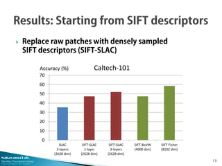
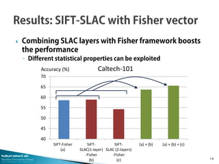
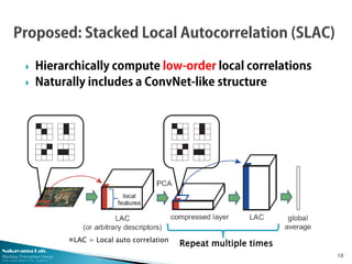
Nakayama Lab.
Machine Perception Group
The University of Tokyo
Grad. School of Information Science and Technology
Hideki Nakayama
Nakayama Lab.
Machine Perception Group
The University of Tokyo
 Deep learning
◦ Successive local response filters and pooling layers
◦ State-of-the-art performance on many tasks & benchmarks
 Traditional BoW-based models are often referred to as
“shallow learning” (interpreted as a single-layer network)
2
[A. Krizhevsky et al., NIPS’12]
Nakayama Lab.
Machine Perception Group
The University of Tokyo
To achieve a certain level of representational power...
 Deep models are believed to require fewer free parameters
or neurons [Larochelle et al., 2007] [Bengio, 2009] [Delalleau and Bengio, 2011]
(not fully proved except for some specific cases, though.)
 However, optimization of deep models is challenging
◦ Non-convex, local minima, many heuristic hyperparameters...
◦ Optimizing shallow network is relatively easy (convex in many cases)
3
(If successfully
trained)  Better generalization
 Computational efficiency
 Scalability
Objection:
“Do Deep Nets Really
Need to be Deep?”
[Ba & Caruana, 2014]
Nakayama Lab.
Machine Perception Group
The University of Tokyo
 Suboptimal (layer-wise)
 Reasonable performance
◦ Even random weights
could work! [Jarrette, 2009]
 Easiness in tuning
 Stability in learning
 Flexibility in the choice of
layer modules
 Global optimality through
the entire network
 State-of-the-art performance
 Difficulty in optimization
 Computational cost
 Constraints on layer modules
4
Fine-tuning (back propagation)
through the entire network is
the key to the best performance!
Structure of the deep network
itself has the primary importance!
Global training of deep models Stacking single-layer
learning modules
◎
◎△
○
Nakayama Lab.
Machine Perception Group
The University of Tokyo
 Suboptimal (layer-wise)
 Reasonable performance
◦ Even random weights
could work! [Jarrette, 2009]
 Easiness in tuning
 Stability in learning
 Flexibility in the choice of
layer modules
 Global optimality through
the entire network
 State-of-the-art performance
 Difficulty in optimization
 Computational cost
 Constraints on layer modules
5
Fine-tuning (back propagation)
through the entire network is
the key to the best performance!
Structure of the deep network
itself has the primary importance!
Global training of deep models Stacking single-layer
learning modules
◎
◎△
○
Nakayama Lab.
Machine Perception Group
The University of Tokyo
Empirically studied on top of the bag-of-words framework
 Hyperfeatures [Agarwal et al., ECCV’06]
◦ Hierarchically stack bag-of-visual-words layers
 Deep Fisher Network [Simonyan et al., NIPS’13]
 Deep Sparse Coding [He et al., SDM’14]
6
Nakayama Lab.
Machine Perception Group
The University of Tokyo
 Higher-order Local Auto-Correlation (HLAC) features
◦ Non-linear filter (mask) response + average pooling
◦ Successfully deployed in many visual recognition applications
 Cons:
◦ Higher-order correlation & masks are required to achieve good
performance, making the feature representation high-dimensional
7
Nakayama Lab.
Machine Perception Group
The University of Tokyo
 Sum-product network [Poon and Domingos, UAI’11]
◦ A deep network where each node (neuron) outputs the sum or
product of input variables
 To represent the same functions, the number of nodes
has to grow: [Delalleau & Bengio, NIPS’11]
◦ Exponentially in a shallow network
◦ Linearly in a deep network
8
Nakayama Lab.
Machine Perception Group
The University of Tokyo
 So, why not use deep models?
9
Nakayama Lab.
Machine Perception Group
The University of Tokyo
 Hierarchically compute low-order local correlations
 Naturally includes a ConvNet-like structure
10
※LAC = Local auto correlation
Repeat multiple times
Nakayama Lab.
Machine Perception Group
The University of Tokyo
 Datasets
◦ MNIST [LeCun,1999]
 Digit recognition
 60k training/10k testing samples
 28x28 pixels
◦ CIFAR-10 [Krizhevsky, 2009]
 Object recognition
 50k training/10k testing samples
 32x32 pixels
◦ Caltech-101 [Fei-Fei, 2004]
 Object recognition
 30 training/15 testing samples
(per class)
 Classifier
◦ Logistic regression
11
Nakayama Lab.
Machine Perception Group
The University of Tokyo
 SLAC achieves better performance than standard
HLAC with reduced feature dimensions
12
84
86
88
90
92
94
96
98
100
HLAC
2nd-order
(35 dim)
HLAC
2nd-order
mask size 5
(219 dim)
HLAC
3rd-order
(153 dim)
HLAC
3rd-order
(2245 dim)
SLAC
2-layers
(1176 dim)
0
10
20
30
40
50
60
70
HLAC
1st-order
(45 dim)
HLAC
2nd-order
(739 dim)
HLAC
2nd-order
mask size 5
(5419 dim)
HLAC
3rd-order
(8023 dim)
SLAC
2-layers
(1176 dim)
Accuracy (%) Accuracy (%)MNIST (gray scale) CIFAR-10 (color)
Nakayama Lab.
Machine Perception Group
The University of Tokyo
 Replace raw patches with densely sampled
SIFT descriptors (SIFT-SLAC)
13
0
10
20
30
40
50
60
70
SLAC
3-layers
(2628 dim)
SIFT-SLAC
1-layer
(2628 dim)
SIFT-SLAC
3-layers
(2628 dim)
SIFT-BoVW
(4000 dim)
SIFT-Fisher
(8192 dim)
Accuracy (%) Caltech-101
Nakayama Lab.
Machine Perception Group
The University of Tokyo
 Combining SLAC layers with Fisher framework boosts
the performance
◦ Different statistical properties can be exploited
14
40
45
50
55
60
65
70
SIFT-Fisher
(a)
SIFT-
SLAC(1-layer)
-Fisher
(b)
SIFT-
SLAC (2-layers)
-Fisher
(c)
(a) + (b) (a) + (b) + (c)
Accuracy (%) Caltech-101
Nakayama Lab.
Machine Perception Group
The University of Tokyo
 Deep learning by stacking is a simple but powerful, flexible
framework to integrate various single-layer modules
 Stacked local autocorrelation (SLAC) features
◦ Iterate computation of local autocorrelation and PCA compression
◦ More efficient than standard HLAC that computes everything in a
single layer
◦ Using multiple layers makes sense
 Learning polynomials is a hot topic in ML
◦ R. Livni et al., Vanishing Component Analysis, In Proc. ICML, 2013.
◦ A. Andoni et al., Learning Polynomials with Neural Networks, In Proc. ICML, 2014.
15

MIRU2014 SLAC

  • 1.
    Nakayama Lab. Machine PerceptionGroup The University of Tokyo The University of Tokyo Grad. School of Information Science and Technology Hideki Nakayama
  • 2.
    Nakayama Lab. Machine PerceptionGroup The University of Tokyo  Deep learning ◦ Successive local response filters and pooling layers ◦ State-of-the-art performance on many tasks & benchmarks  Traditional BoW-based models are often referred to as “shallow learning” (interpreted as a single-layer network) 2 [A. Krizhevsky et al., NIPS’12]
  • 3.
    Nakayama Lab. Machine PerceptionGroup The University of Tokyo To achieve a certain level of representational power...  Deep models are believed to require fewer free parameters or neurons [Larochelle et al., 2007] [Bengio, 2009] [Delalleau and Bengio, 2011] (not fully proved except for some specific cases, though.)  However, optimization of deep models is challenging ◦ Non-convex, local minima, many heuristic hyperparameters... ◦ Optimizing shallow network is relatively easy (convex in many cases) 3 (If successfully trained)  Better generalization  Computational efficiency  Scalability Objection: “Do Deep Nets Really Need to be Deep?” [Ba & Caruana, 2014]
  • 4.
    Nakayama Lab. Machine PerceptionGroup The University of Tokyo  Suboptimal (layer-wise)  Reasonable performance ◦ Even random weights could work! [Jarrette, 2009]  Easiness in tuning  Stability in learning  Flexibility in the choice of layer modules  Global optimality through the entire network  State-of-the-art performance  Difficulty in optimization  Computational cost  Constraints on layer modules 4 Fine-tuning (back propagation) through the entire network is the key to the best performance! Structure of the deep network itself has the primary importance! Global training of deep models Stacking single-layer learning modules ◎ ◎△ ○
  • 5.
    Nakayama Lab. Machine PerceptionGroup The University of Tokyo  Suboptimal (layer-wise)  Reasonable performance ◦ Even random weights could work! [Jarrette, 2009]  Easiness in tuning  Stability in learning  Flexibility in the choice of layer modules  Global optimality through the entire network  State-of-the-art performance  Difficulty in optimization  Computational cost  Constraints on layer modules 5 Fine-tuning (back propagation) through the entire network is the key to the best performance! Structure of the deep network itself has the primary importance! Global training of deep models Stacking single-layer learning modules ◎ ◎△ ○
  • 6.
    Nakayama Lab. Machine PerceptionGroup The University of Tokyo Empirically studied on top of the bag-of-words framework  Hyperfeatures [Agarwal et al., ECCV’06] ◦ Hierarchically stack bag-of-visual-words layers  Deep Fisher Network [Simonyan et al., NIPS’13]  Deep Sparse Coding [He et al., SDM’14] 6
  • 7.
    Nakayama Lab. Machine PerceptionGroup The University of Tokyo  Higher-order Local Auto-Correlation (HLAC) features ◦ Non-linear filter (mask) response + average pooling ◦ Successfully deployed in many visual recognition applications  Cons: ◦ Higher-order correlation & masks are required to achieve good performance, making the feature representation high-dimensional 7
  • 8.
    Nakayama Lab. Machine PerceptionGroup The University of Tokyo  Sum-product network [Poon and Domingos, UAI’11] ◦ A deep network where each node (neuron) outputs the sum or product of input variables  To represent the same functions, the number of nodes has to grow: [Delalleau & Bengio, NIPS’11] ◦ Exponentially in a shallow network ◦ Linearly in a deep network 8
  • 9.
    Nakayama Lab. Machine PerceptionGroup The University of Tokyo  So, why not use deep models? 9
  • 10.
    Nakayama Lab. Machine PerceptionGroup The University of Tokyo  Hierarchically compute low-order local correlations  Naturally includes a ConvNet-like structure 10 ※LAC = Local auto correlation Repeat multiple times
  • 11.
    Nakayama Lab. Machine PerceptionGroup The University of Tokyo  Datasets ◦ MNIST [LeCun,1999]  Digit recognition  60k training/10k testing samples  28x28 pixels ◦ CIFAR-10 [Krizhevsky, 2009]  Object recognition  50k training/10k testing samples  32x32 pixels ◦ Caltech-101 [Fei-Fei, 2004]  Object recognition  30 training/15 testing samples (per class)  Classifier ◦ Logistic regression 11
  • 12.
    Nakayama Lab. Machine PerceptionGroup The University of Tokyo  SLAC achieves better performance than standard HLAC with reduced feature dimensions 12 84 86 88 90 92 94 96 98 100 HLAC 2nd-order (35 dim) HLAC 2nd-order mask size 5 (219 dim) HLAC 3rd-order (153 dim) HLAC 3rd-order (2245 dim) SLAC 2-layers (1176 dim) 0 10 20 30 40 50 60 70 HLAC 1st-order (45 dim) HLAC 2nd-order (739 dim) HLAC 2nd-order mask size 5 (5419 dim) HLAC 3rd-order (8023 dim) SLAC 2-layers (1176 dim) Accuracy (%) Accuracy (%)MNIST (gray scale) CIFAR-10 (color)
  • 13.
    Nakayama Lab. Machine PerceptionGroup The University of Tokyo  Replace raw patches with densely sampled SIFT descriptors (SIFT-SLAC) 13 0 10 20 30 40 50 60 70 SLAC 3-layers (2628 dim) SIFT-SLAC 1-layer (2628 dim) SIFT-SLAC 3-layers (2628 dim) SIFT-BoVW (4000 dim) SIFT-Fisher (8192 dim) Accuracy (%) Caltech-101
  • 14.
    Nakayama Lab. Machine PerceptionGroup The University of Tokyo  Combining SLAC layers with Fisher framework boosts the performance ◦ Different statistical properties can be exploited 14 40 45 50 55 60 65 70 SIFT-Fisher (a) SIFT- SLAC(1-layer) -Fisher (b) SIFT- SLAC (2-layers) -Fisher (c) (a) + (b) (a) + (b) + (c) Accuracy (%) Caltech-101
  • 15.
    Nakayama Lab. Machine PerceptionGroup The University of Tokyo  Deep learning by stacking is a simple but powerful, flexible framework to integrate various single-layer modules  Stacked local autocorrelation (SLAC) features ◦ Iterate computation of local autocorrelation and PCA compression ◦ More efficient than standard HLAC that computes everything in a single layer ◦ Using multiple layers makes sense  Learning polynomials is a hot topic in ML ◦ R. Livni et al., Vanishing Component Analysis, In Proc. ICML, 2013. ◦ A. Andoni et al., Learning Polynomials with Neural Networks, In Proc. ICML, 2014. 15