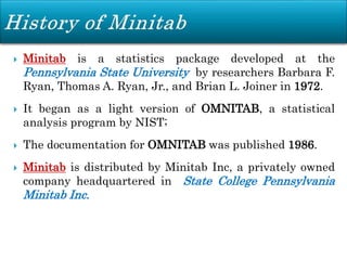
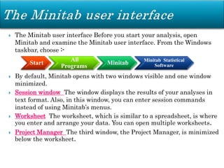
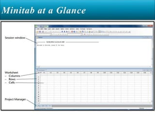
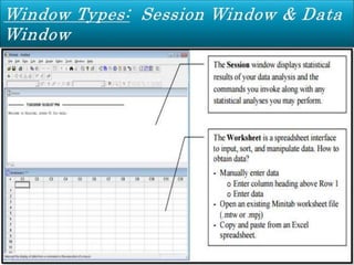
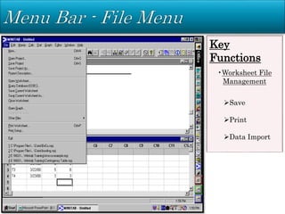
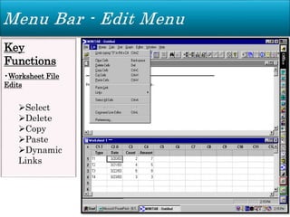
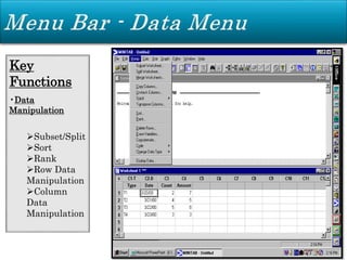
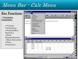
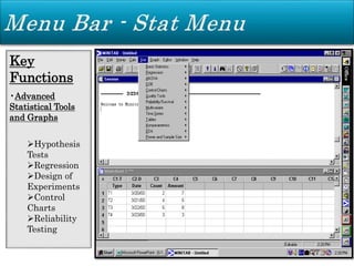
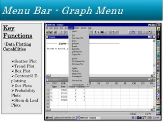
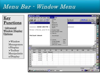
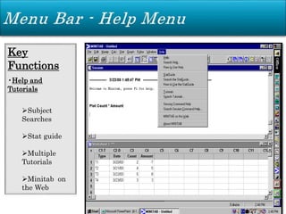
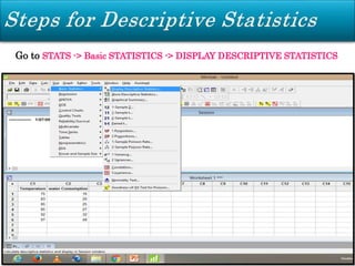
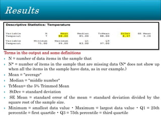
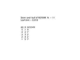
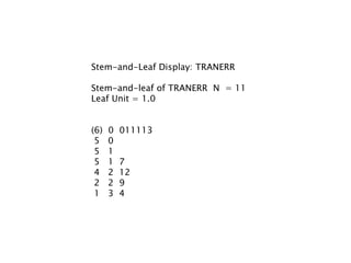
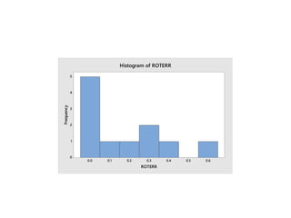
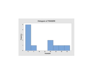
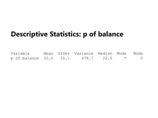
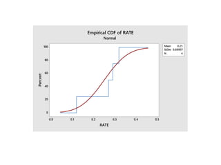
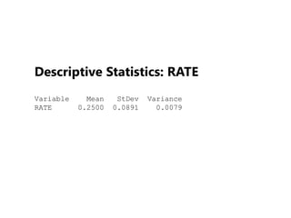
Presenting by
Marwah Saeb Kadhim
Dhay saeb kadhim
Safa falih kareem
Headline
Introduction to Minitab
History of Minitab
The Minitab user interface
Minitab at a Glance
 Minitab, originally intended as a tool for
teaching statistics, is a general-purpose
statistical software package designed for
easy interactive use.
 Minitab is well suited for instructional
applications, but is also powerful enough to
be used as a primary tool for analyzing
research data.
 Minitab is a statistics package developed at the
Pennsylvania State University by researchers Barbara F.
Ryan, Thomas A. Ryan, Jr., and Brian L. Joiner in 1972.
 It began as a light version of OMNITAB, a statistical
analysis program by NIST;
 The documentation for OMNITAB was published 1986.
 Minitab is distributed by Minitab Inc, a privately owned
company headquartered in State College Pennsylvania
Minitab Inc.
 The Minitab user interface Before you start your analysis, open
Minitab and examine the Minitab user interface. From the Windows
taskbar, choose :-
 By default, Minitab opens with two windows visible and one window
minimized.
 Session window The window displays the results of your analyses in
text format. Also, in this window, you can enter session commands
instead of using Minitab’s menus.
 Worksheet The worksheet, which is similar to a spreadsheet, is where
you enter and arrange your data. You can open multiple worksheets.
 Project Manager The third window, the Project Manager, is minimized
below the worksheet.
Start
All
Programs
Minitab Minitab Statistical
Software
Key
Functions
•Worksheet File
Management
Save
Print
Data Import
Key
Functions
•Worksheet File
Edits
Select
Delete
Copy
Paste
Dynamic
Links
Key
Functions
•Data
Manipulation
Subset/Split
Sort
Rank
Row Data
Manipulation
Column
Data
Manipulation
Key Functions
•Calculation
Capabilities
Column
Calculations
Column/Row
Statistics
Data
Standardization
Data Extraction
Data
Generation
Key
Functions
•Advanced
Statistical Tools
and Graphs
Hypothesis
Tests
Regression
Design of
Experiments
Control
Charts
Reliability
Testing
Key
Functions
•Data Plotting
Capabilities
Scatter Plot
Trend Plot
Box Plot
Contour/3 D
plotting
Dot Plots
Probability
Plots
Stem & Leaf
Plots
Key
Functions
•Advanced Edit
and Display
Options
Font
Connectivit
y Settings
Key
Functions
•Advanced
Window Display
Options
Window
Managemen
t/Display
Toolbar
Manipulatio
n/Display
Key
Functions
•Help and
Tutorials
Subject
Searches
Stat guide
Multiple
Tutorials
Minitab on
the Web
 Numerical: Numerical data is the only type Minitab will use
for statistical calculations. Numerical data is aligned on the
right side of the column. Minitab will not recognize numbers
with commas as numbers, but as text.
 Text: Text cannot be used for computations. Though “text”
generally means words or characters, numbers can be
classified as text. If column 1 has text in it, the column label
will change from C1 to C1-T. Data types can be changed.
 Date/Time: Minitab recognizes 3/5/00 as a date, but will store
this internally as a number so you can manipulate it. The
column label will indicate a date by C1-D and a time by C1-T.
Examine worksheet
The data are arranged in columns, which are also called variables. The
column number and name are at the top of each column. Each row in
the worksheet represents a case, which is information on a single book
order.
Column with text data
Column with numeric data
Column with
date/time data
Column
name
Row
number
 Within a project you can open one or more files that contain data. When
you open a file, you copy the contents of the file into the current Minitab
project.
 To open a Minitab type file
◦ Choose FILE -> OPEN WORKSHEET
◦ Look for the file you want to open. Should be a .MTW or .MPJ type file.
Select the file and click Open.
◦ If you get a message box indicating that the content of the file will be
added to the current project, check “Do not display this message
again”.
◦ Click OK.
 Opening Excel files
◦ Choose FILE -> OPEN
WORKSHEET
◦ In the field “File of Type”
select EXCEL (*.xls,
*.xlsx) from the drop down
menu.
◦ Choose the file you wish
to open, and click Open.
 Copying data to Minitab works like copying data to any
other type of spreadsheet (eg. Excel).
◦ Copy the data you wish to use in Minitab.
◦ Go to the position where you want to copy the data in the
desired Minitab worksheet. If you wish to paste a cell
with a Header or Name, make sure that you stand in the
variable name cell (cell below the number of the column
C1, C2, etc).
◦ Go to EDIT -> PASTE CELLS to paste the data.
◦ Sometimes when you copy data, Minitab reads it in a
wrong format, eg. As a text when is numeric. To solve
this problem, select the problematic column(s) and go to
DATA -> CHANGE DATA TYPE -> CHOOSE THE
DESIRED FORMAT. The most useful format is numeric.
The following dialog box appears. Choose the variables you want to
modify and where you want to store them. The storage variables can be
the same variables as the ones you are modifying.
Then hit OK.
 You can save two different things in Minitab. You can save the
worksheet by itself, or the entire project. Saving the
worksheet as a separate file is a very good habit. That way
you have the data stored in a place where you can always go
back to it, even if the data you are working with in a given
project is corrupted. To save the data in a worksheet by itself,
◦ 1. Select FILE > SAVE CURRENT WORKSHEET AS.
◦ 2. Use the arrow beside the Save in field to select the Floppy (A)
or location of your disk.
◦ 3. In the File Name field type the name of the worksheet. Minitab
will automatically add the extension MTW for Minitab worksheet.
◦ 4. Click Save.
 Minitab allows you to do calculations with the variables that
you are using. For example you can add and multiply
variables.
 In order to do these calculations you should go to CALC ->
CALCULATOR
 The following dialog box appears
This is basically a calculator
that allows doing many
calculations with the variables.
Basic functions are found in the
number pad and more
sophisticated ones are found in
the functions box to the right of
the number pad.
 To make sure that your results
is not overwriting a variable,
name a new variable in the
“STORE RESULTS IN
VAVRIABLE” field in the top of
the calculator.
 To add variables name the
variable where you want to store
the results.
 Select the first variable, press
the “+” sign and select the
second variable (and so on for
more than two variables). You
should obtain something similar
to the window in the right
 The result will appear in the worksheet window.
 You can enter data in a Minitab worksheet in the
following ways:
◦ Type the data directly into the worksheet.
◦ Copy and paste the data from other applications.
◦ Import the data from Microsoft Excel files or text files.
After your data are in Minitab, you might need to
edit cells or reorganize columns and rows to prepare
the data for analysis. Some common manipulations
are stacking, sub setting, specifying column names,
and editing data values.
Descriptive statistics are brief descriptive coefficients
that summarize a given data set, which can be either a
representation of the entire population or a sample of it.
Descriptive statistics are broken down into measures of
central tendency and measures of variability, or spread.
Measures of central tendency include the mean, median
and mode, while measures of variability include
the standard deviation or variance, the minimum and
maximum variables, and the kurtosis and skewness.
 Central Tendency. The central tendency of a distribution is
an estimate of the "center" of a distribution of values.
There are three major types of estimates of central
tendency:
◦ Mean
◦ Median
◦ Mode
 Dispersion. Dispersion refers to the spread of the values
around the central tendency.
◦ Standard Deviation
◦ Range
 Mean or average is probably the most commonly used
method of describing central tendency. To compute the
mean all you do is add up all the values and divide by
the number of values.
◦ For example, the mean or average quiz score is determined by
summing all the scores and dividing by the number of students
taking the exam. For example, consider the test score values:
15, 20, 21, 20, 36, 15, 25, 15
The sum of these 8 values is 167, so the mean is 167/8 = 20.875.
 The Median is the score found at the exact middle of the
set of values. One way to compute the median is to list all
scores in numerical order, and then locate the score in the
center of the sample.
◦ For example, if there are 500 scores in the list, score #250
would be the median. If we order the 8 scores shown above, we
would get:
15,15,15,20,20,21,25,36
◦ There are 8 scores and score #4 and #5 represent the halfway
point. Since both of these scores are 20, the median is 20. If the
two middle scores had different values, you would have to
interpolate to determine the median.
 The mode is the most frequently occurring value in the set of
scores. To determine the mode, you might again order the scores
as shown above, and then count each one. The most frequently
occurring value is the mode.
◦ In our example, the value 15 occurs three times and is the model. In
some distributions there is more than one modal value. For instance,
in a bimodal distribution there are two values that occur most
frequently.
 Notice that for the same set of 8 scores we got three different
values -- 20.875, 20, and 15 -- for the mean, median and mode
respectively. If the distribution is truly normal (i.e., bell-shaped),
the mean, median and mode are all equal to each other.
 The standard deviation is a measure of the spread of scores
within a set of data.
 The sample standard deviation formula is:
The population standard deviation formula is:
where
s = sample standard deviation
n = number of scores in sample.
X =Sample Mean
σ = population standard deviation
Enter the column headings.
Column headings must be entered above Row 1.
Example:
 Enter “Temperature (F)” in the first cell in Column 1.
*The first cell is above Row 1.
 Enter “Water Consumption (ounces)” in first cell in
Column 2. *The first cell is above Row 2. Enter the
data.
 Enter the corresponding temperatures and water
consumption in the appropriate column as shown. Do
not change the order of the items. Make sure the
items were entered as numbers not text.
Go to STATS -> Basic STATISTICS -> DISPLAY DESCRIPTIVE STATISTICS
2. And a prompt window should appear. In the window select the
variable(s) you want to analyze and click ok.
In the Variables box, select C1 (Temperature).
3. Click OK.
4. Look in the Session window. You should see the following display
Terms in the output and some definitions
 N = number of data items in the sample that
 N* = number of items in the sample that are missing data (N* does not show up
when all the items in the sample have data, as in our example.)
 Mean = "average"
 Median = "middle number"
 TrMean= the 5% Trimmed Mean
 StDev = standard deviation
 SE Mean = standard error of the mean = standard deviation divided by the
square root of the sample size.
 Minimum = smallest data value • Maximum = largest data value • Q1 = 25th
percentile = first quartile • Q3 = 75th percentile = third quartile
Go to STATS -> Graphical Summary
2. And a prompt window should appear. In the window select the
variable(s) you want to analyze and click ok.
In the Variables box, select C1 (Temperature).
3. Click OK.
4. Look in the Session window. You should see the following display
 Select FILE > SAVE CURRENT WORKSHEET AS.
 Use the arrow beside the Save in field to select the
Floppy (A) or location of your diskette.
 In the File Name field type the name of the
worksheet. Minitab will automatically add the
extension MTW for Minitab worksheet.
 Click Save
Example 1 :- Unauthorized computer use. The Computer Security Institute (CSI)
conducts an annual survey of computer crime at U.S. businesses. CSI sends
survey questionnaires to computer security personnel at all U.S. corporations
and government agencies. In 2001, 64% of the respondents admitted
unauthorized use of computer systems at their firms during the year.
(Computer Security Issues & Trends, Spring 2001.) One survey question
asked, “If your business
website suffered unauthorized use, where did the attack come from, inside or
outside the company?” The responses for those business websites that did, in
fact, experience unauthorized use are summarized in the table for
two survey years, 1999 (125 reported attacks) and 2001
(163 reported attacks).
a. Construct a bar chart to describe the sources of unauthorized computer
use in 1999.
b. Construct a bar chart to describe the sources of unauthorized
computer use in 2001.
C. Find the mean ,standard devision ,minimum and maximum for both
source in 1999 and 2001.
WWW SITE ATTACK PERCENTAGE
IN 1999
PERCENTAGE
IN 2001
INSIDE 7 4
OUTSIDE 38 47
BOTH 41 23
DONOT KNOW 14 26
TOTALS 100 100
EXAMPLE 2:- sensor motion of a robot . Rescrchers at Carnegie Mellon
university developed an algorithm for estimating the scnsor motion of a
robotic arm by mounting a camera with inertia sensors on the arm (the
international journal of robotics research ,Dec.2004. )two variables of interest
were the error of estimating arm rotation (measured in radians )and the error
of estimating arm translation (measured in centimeters).data for 11
expeirments are listed in the table .in each experiment .the perturbation of
camera intrinsics and projections were varied .
a. Construct a dot plot for the 11 measurements.
b. Construct a stem-and-leaf display for the 11 measurements.
c. Construct a histogram plot for the 11 measurements.
35
30
25
20
15
10
5
0
TRANERR
Dotplot of TRANERR
0.56
0.48
0.40
0.32
0.24
0.16
0.08
0.00
ROTERR
Dotplot of ROTERR
Stem-and-leaf of ROTERR N = 11
Leaf Unit = 0.010
(6) 0 023349
5 1 9
4 2 7
3 3 2
2 4 2
1 5 7
Stem-and-Leaf Display: TRANERR
Stem-and-leaf of TRANERR N = 11
Leaf Unit = 1.0
(6) 0 011113
5 0
5 1
5 1 7
4 2 12
2 2 9
1 3 4
0.6
0.5
0.4
0.3
0.2
0.1
0.0
5
4
3
2
1
0
ROTERR
Frequency Histogram of ROTERR
35
30
25
20
15
10
5
0
5
4
3
2
1
0
TRANERR
Frequency Histogram of TRANERR
EXAMPLE 3 : Controlling water hyacinth. Refer to the Annals of the
Entomological Society of America (Jan. 2005) study of
the life cycle of a South American delphacid species, Exercise
4.3 (p. 138). Recall that entomological engineers
have found that the delphacid is a natural enemy of water
hyacinth. The table giving the percentages of water hyacinth
blades that have one, two, three, and four delphacid
eggs is reproduced here. Consider a sample of
100 water hyacinth blades selected from an environment
inhabited by delphacids. Let Y1, Y2, Y3, and Y4 represent
the number of blades in the sample with one egg, two
eggs, three eggs, and four eggs, respectively. Find the
probability that half of the sampled blades have one egg,
half have two eggs, and none of the blades has three or
four eggs
One eggs Two eggs Three eggs Four eggs
% of blades 40 54 2 4
Descriptive Statistics: p of balance
Variable Mean StDev Variance Median Mode Mode
p of balance 25.0 26.1 678.7 22.0 * 0
4
3
2
1
60
50
40
30
20
10
0
Index
p
of
balance
Area Graph of p of balance
Example:Management system failures. Refer to the Process Safety
Progress (Dec., 2004) study of industrial accidents caused
by management system failures, Exercise 3.78 (p. 127).
The table listing the four root causes of system failures
(and associated proportions) is reproduced below. Suppose
three industrial accidents are randomly selected
(without replacement) from among all industrial accidents
caused by management system failures. Find and graph
the probability distribution of Y, the number of accidents
caused by Engineering and Design failure.
CAUSE CATEEGORY
PROPRTION
ENGEENRING .32
PROCDURES .29
MANAGEMENT .27
TRAINING .12
TOTAL 1
0.5
0.4
0.3
0.2
0.1
0.0
100
80
60
40
20
0
Mean 0.25
StDev 0.08907
N 4
RATE
Percent
Empirical CDF of RATE
Normal
Descriptive Statistics: RATE
Variable Mean StDev Variance
RATE 0.2500 0.0891 0.0079
Minitab Seminar1.pptx

Minitab Seminar1.pptx

  • 1.
    Presenting by Marwah SaebKadhim Dhay saeb kadhim Safa falih kareem
  • 2.
    Headline Introduction to Minitab Historyof Minitab The Minitab user interface Minitab at a Glance
  • 3.
     Minitab, originallyintended as a tool for teaching statistics, is a general-purpose statistical software package designed for easy interactive use.  Minitab is well suited for instructional applications, but is also powerful enough to be used as a primary tool for analyzing research data.
  • 4.
     Minitab isa statistics package developed at the Pennsylvania State University by researchers Barbara F. Ryan, Thomas A. Ryan, Jr., and Brian L. Joiner in 1972.  It began as a light version of OMNITAB, a statistical analysis program by NIST;  The documentation for OMNITAB was published 1986.  Minitab is distributed by Minitab Inc, a privately owned company headquartered in State College Pennsylvania Minitab Inc.
  • 5.
     The Minitabuser interface Before you start your analysis, open Minitab and examine the Minitab user interface. From the Windows taskbar, choose :-  By default, Minitab opens with two windows visible and one window minimized.  Session window The window displays the results of your analyses in text format. Also, in this window, you can enter session commands instead of using Minitab’s menus.  Worksheet The worksheet, which is similar to a spreadsheet, is where you enter and arrange your data. You can open multiple worksheets.  Project Manager The third window, the Project Manager, is minimized below the worksheet. Start All Programs Minitab Minitab Statistical Software
  • 8.
  • 9.
  • 10.
  • 11.
  • 12.
  • 13.
    Key Functions •Data Plotting Capabilities Scatter Plot TrendPlot Box Plot Contour/3 D plotting Dot Plots Probability Plots Stem & Leaf Plots
  • 14.
  • 15.
  • 16.
  • 17.
     Numerical: Numericaldata is the only type Minitab will use for statistical calculations. Numerical data is aligned on the right side of the column. Minitab will not recognize numbers with commas as numbers, but as text.  Text: Text cannot be used for computations. Though “text” generally means words or characters, numbers can be classified as text. If column 1 has text in it, the column label will change from C1 to C1-T. Data types can be changed.  Date/Time: Minitab recognizes 3/5/00 as a date, but will store this internally as a number so you can manipulate it. The column label will indicate a date by C1-D and a time by C1-T.
  • 18.
    Examine worksheet The dataare arranged in columns, which are also called variables. The column number and name are at the top of each column. Each row in the worksheet represents a case, which is information on a single book order. Column with text data Column with numeric data Column with date/time data Column name Row number
  • 19.
     Within aproject you can open one or more files that contain data. When you open a file, you copy the contents of the file into the current Minitab project.  To open a Minitab type file ◦ Choose FILE -> OPEN WORKSHEET ◦ Look for the file you want to open. Should be a .MTW or .MPJ type file. Select the file and click Open. ◦ If you get a message box indicating that the content of the file will be added to the current project, check “Do not display this message again”. ◦ Click OK.
  • 20.
     Opening Excelfiles ◦ Choose FILE -> OPEN WORKSHEET ◦ In the field “File of Type” select EXCEL (*.xls, *.xlsx) from the drop down menu. ◦ Choose the file you wish to open, and click Open.
  • 21.
     Copying datato Minitab works like copying data to any other type of spreadsheet (eg. Excel). ◦ Copy the data you wish to use in Minitab. ◦ Go to the position where you want to copy the data in the desired Minitab worksheet. If you wish to paste a cell with a Header or Name, make sure that you stand in the variable name cell (cell below the number of the column C1, C2, etc). ◦ Go to EDIT -> PASTE CELLS to paste the data. ◦ Sometimes when you copy data, Minitab reads it in a wrong format, eg. As a text when is numeric. To solve this problem, select the problematic column(s) and go to DATA -> CHANGE DATA TYPE -> CHOOSE THE DESIRED FORMAT. The most useful format is numeric.
  • 22.
    The following dialogbox appears. Choose the variables you want to modify and where you want to store them. The storage variables can be the same variables as the ones you are modifying. Then hit OK.
  • 23.
     You cansave two different things in Minitab. You can save the worksheet by itself, or the entire project. Saving the worksheet as a separate file is a very good habit. That way you have the data stored in a place where you can always go back to it, even if the data you are working with in a given project is corrupted. To save the data in a worksheet by itself, ◦ 1. Select FILE > SAVE CURRENT WORKSHEET AS. ◦ 2. Use the arrow beside the Save in field to select the Floppy (A) or location of your disk. ◦ 3. In the File Name field type the name of the worksheet. Minitab will automatically add the extension MTW for Minitab worksheet. ◦ 4. Click Save.
  • 24.
     Minitab allowsyou to do calculations with the variables that you are using. For example you can add and multiply variables.  In order to do these calculations you should go to CALC -> CALCULATOR
  • 25.
     The followingdialog box appears This is basically a calculator that allows doing many calculations with the variables. Basic functions are found in the number pad and more sophisticated ones are found in the functions box to the right of the number pad.  To make sure that your results is not overwriting a variable, name a new variable in the “STORE RESULTS IN VAVRIABLE” field in the top of the calculator.
  • 26.
     To addvariables name the variable where you want to store the results.  Select the first variable, press the “+” sign and select the second variable (and so on for more than two variables). You should obtain something similar to the window in the right
  • 27.
     The resultwill appear in the worksheet window.
  • 29.
     You canenter data in a Minitab worksheet in the following ways: ◦ Type the data directly into the worksheet. ◦ Copy and paste the data from other applications. ◦ Import the data from Microsoft Excel files or text files. After your data are in Minitab, you might need to edit cells or reorganize columns and rows to prepare the data for analysis. Some common manipulations are stacking, sub setting, specifying column names, and editing data values.
  • 31.
    Descriptive statistics arebrief descriptive coefficients that summarize a given data set, which can be either a representation of the entire population or a sample of it. Descriptive statistics are broken down into measures of central tendency and measures of variability, or spread. Measures of central tendency include the mean, median and mode, while measures of variability include the standard deviation or variance, the minimum and maximum variables, and the kurtosis and skewness.
  • 32.
     Central Tendency.The central tendency of a distribution is an estimate of the "center" of a distribution of values. There are three major types of estimates of central tendency: ◦ Mean ◦ Median ◦ Mode  Dispersion. Dispersion refers to the spread of the values around the central tendency. ◦ Standard Deviation ◦ Range
  • 33.
     Mean oraverage is probably the most commonly used method of describing central tendency. To compute the mean all you do is add up all the values and divide by the number of values. ◦ For example, the mean or average quiz score is determined by summing all the scores and dividing by the number of students taking the exam. For example, consider the test score values: 15, 20, 21, 20, 36, 15, 25, 15 The sum of these 8 values is 167, so the mean is 167/8 = 20.875.
  • 34.
     The Medianis the score found at the exact middle of the set of values. One way to compute the median is to list all scores in numerical order, and then locate the score in the center of the sample. ◦ For example, if there are 500 scores in the list, score #250 would be the median. If we order the 8 scores shown above, we would get: 15,15,15,20,20,21,25,36 ◦ There are 8 scores and score #4 and #5 represent the halfway point. Since both of these scores are 20, the median is 20. If the two middle scores had different values, you would have to interpolate to determine the median.
  • 35.
     The modeis the most frequently occurring value in the set of scores. To determine the mode, you might again order the scores as shown above, and then count each one. The most frequently occurring value is the mode. ◦ In our example, the value 15 occurs three times and is the model. In some distributions there is more than one modal value. For instance, in a bimodal distribution there are two values that occur most frequently.  Notice that for the same set of 8 scores we got three different values -- 20.875, 20, and 15 -- for the mean, median and mode respectively. If the distribution is truly normal (i.e., bell-shaped), the mean, median and mode are all equal to each other.
  • 36.
     The standarddeviation is a measure of the spread of scores within a set of data.  The sample standard deviation formula is: The population standard deviation formula is: where s = sample standard deviation n = number of scores in sample. X =Sample Mean σ = population standard deviation
  • 37.
    Enter the columnheadings. Column headings must be entered above Row 1. Example:  Enter “Temperature (F)” in the first cell in Column 1. *The first cell is above Row 1.  Enter “Water Consumption (ounces)” in first cell in Column 2. *The first cell is above Row 2. Enter the data.  Enter the corresponding temperatures and water consumption in the appropriate column as shown. Do not change the order of the items. Make sure the items were entered as numbers not text.
  • 38.
    Go to STATS-> Basic STATISTICS -> DISPLAY DESCRIPTIVE STATISTICS
  • 39.
    2. And aprompt window should appear. In the window select the variable(s) you want to analyze and click ok. In the Variables box, select C1 (Temperature). 3. Click OK.
  • 40.
    4. Look inthe Session window. You should see the following display
  • 41.
    Terms in theoutput and some definitions  N = number of data items in the sample that  N* = number of items in the sample that are missing data (N* does not show up when all the items in the sample have data, as in our example.)  Mean = "average"  Median = "middle number"  TrMean= the 5% Trimmed Mean  StDev = standard deviation  SE Mean = standard error of the mean = standard deviation divided by the square root of the sample size.  Minimum = smallest data value • Maximum = largest data value • Q1 = 25th percentile = first quartile • Q3 = 75th percentile = third quartile
  • 42.
    Go to STATS-> Graphical Summary
  • 43.
    2. And aprompt window should appear. In the window select the variable(s) you want to analyze and click ok. In the Variables box, select C1 (Temperature). 3. Click OK.
  • 44.
    4. Look inthe Session window. You should see the following display
  • 45.
     Select FILE> SAVE CURRENT WORKSHEET AS.  Use the arrow beside the Save in field to select the Floppy (A) or location of your diskette.  In the File Name field type the name of the worksheet. Minitab will automatically add the extension MTW for Minitab worksheet.  Click Save
  • 46.
    Example 1 :-Unauthorized computer use. The Computer Security Institute (CSI) conducts an annual survey of computer crime at U.S. businesses. CSI sends survey questionnaires to computer security personnel at all U.S. corporations and government agencies. In 2001, 64% of the respondents admitted unauthorized use of computer systems at their firms during the year. (Computer Security Issues & Trends, Spring 2001.) One survey question asked, “If your business website suffered unauthorized use, where did the attack come from, inside or outside the company?” The responses for those business websites that did, in fact, experience unauthorized use are summarized in the table for two survey years, 1999 (125 reported attacks) and 2001 (163 reported attacks). a. Construct a bar chart to describe the sources of unauthorized computer use in 1999. b. Construct a bar chart to describe the sources of unauthorized computer use in 2001. C. Find the mean ,standard devision ,minimum and maximum for both source in 1999 and 2001.
  • 47.
    WWW SITE ATTACKPERCENTAGE IN 1999 PERCENTAGE IN 2001 INSIDE 7 4 OUTSIDE 38 47 BOTH 41 23 DONOT KNOW 14 26 TOTALS 100 100
  • 54.
    EXAMPLE 2:- sensormotion of a robot . Rescrchers at Carnegie Mellon university developed an algorithm for estimating the scnsor motion of a robotic arm by mounting a camera with inertia sensors on the arm (the international journal of robotics research ,Dec.2004. )two variables of interest were the error of estimating arm rotation (measured in radians )and the error of estimating arm translation (measured in centimeters).data for 11 expeirments are listed in the table .in each experiment .the perturbation of camera intrinsics and projections were varied .
  • 55.
    a. Construct adot plot for the 11 measurements. b. Construct a stem-and-leaf display for the 11 measurements. c. Construct a histogram plot for the 11 measurements.
  • 57.
  • 58.
  • 59.
    Stem-and-leaf of ROTERRN = 11 Leaf Unit = 0.010 (6) 0 023349 5 1 9 4 2 7 3 3 2 2 4 2 1 5 7
  • 60.
    Stem-and-Leaf Display: TRANERR Stem-and-leafof TRANERR N = 11 Leaf Unit = 1.0 (6) 0 011113 5 0 5 1 5 1 7 4 2 12 2 2 9 1 3 4
  • 61.
  • 62.
  • 63.
    EXAMPLE 3 :Controlling water hyacinth. Refer to the Annals of the Entomological Society of America (Jan. 2005) study of the life cycle of a South American delphacid species, Exercise 4.3 (p. 138). Recall that entomological engineers have found that the delphacid is a natural enemy of water hyacinth. The table giving the percentages of water hyacinth blades that have one, two, three, and four delphacid eggs is reproduced here. Consider a sample of 100 water hyacinth blades selected from an environment inhabited by delphacids. Let Y1, Y2, Y3, and Y4 represent the number of blades in the sample with one egg, two eggs, three eggs, and four eggs, respectively. Find the probability that half of the sampled blades have one egg, half have two eggs, and none of the blades has three or four eggs One eggs Two eggs Three eggs Four eggs % of blades 40 54 2 4
  • 66.
    Descriptive Statistics: pof balance Variable Mean StDev Variance Median Mode Mode p of balance 25.0 26.1 678.7 22.0 * 0
  • 67.
  • 68.
    Example:Management system failures.Refer to the Process Safety Progress (Dec., 2004) study of industrial accidents caused by management system failures, Exercise 3.78 (p. 127). The table listing the four root causes of system failures (and associated proportions) is reproduced below. Suppose three industrial accidents are randomly selected (without replacement) from among all industrial accidents caused by management system failures. Find and graph the probability distribution of Y, the number of accidents caused by Engineering and Design failure.
  • 69.
    CAUSE CATEEGORY PROPRTION ENGEENRING .32 PROCDURES.29 MANAGEMENT .27 TRAINING .12 TOTAL 1
  • 71.
  • 72.
    Descriptive Statistics: RATE VariableMean StDev Variance RATE 0.2500 0.0891 0.0079