Download to read offline

![Symbol Reference . . . . . . . . . . . . . . . . . . . . . . . . . . . . . . . . . 2-74
Asterisk — * . . . . . . . . . . . . . . . . . . . . . . . . . . . . . . . . . . . . . 2-74
At — @ . . . . . . . . . . . . . . . . . . . . . . . . . . . . . . . . . . . . . . . . . . 2-75
Colon — : . . . . . . . . . . . . . . . . . . . . . . . . . . . . . . . . . . . . . . . . 2-76
Comma — , . . . . . . . . . . . . . . . . . . . . . . . . . . . . . . . . . . . . . . 2-77
Curly Braces — { } . . . . . . . . . . . . . . . . . . . . . . . . . . . . . . . . . 2-78
Dot — . . . . . . . . . . . . . . . . . . . . . . . . . . . . . . . . . . . . . . . . . . . 2-78
Dot-Dot — .. . . . . . . . . . . . . . . . . . . . . . . . . . . . . . . . . . . . . . . 2-79
Dot-Dot-Dot (Ellipsis) — ... . . . . . . . . . . . . . . . . . . . . . . . . . . 2-79
Dot-Parentheses — .( ) . . . . . . . . . . . . . . . . . . . . . . . . . . . . . 2-80
Exclamation Point — ! . . . . . . . . . . . . . . . . . . . . . . . . . . . . . 2-81
Parentheses — ( ) . . . . . . . . . . . . . . . . . . . . . . . . . . . . . . . . . 2-81
Percent — % . . . . . . . . . . . . . . . . . . . . . . . . . . . . . . . . . . . . . 2-82
Percent-Brace — %{ %} . . . . . . . . . . . . . . . . . . . . . . . . . . . . . 2-82
Plus — + . . . . . . . . . . . . . . . . . . . . . . . . . . . . . . . . . . . . . . . . . 2-83
Semicolon — ; . . . . . . . . . . . . . . . . . . . . . . . . . . . . . . . . . . . . 2-83
Single Quotes — ’ ’ . . . . . . . . . . . . . . . . . . . . . . . . . . . . . . . . . 2-84
Space Character . . . . . . . . . . . . . . . . . . . . . . . . . . . . . . . . . . 2-84
Slash and Backslash — / . . . . . . . . . . . . . . . . . . . . . . . . . . 2-85
Square Brackets — [ ] . . . . . . . . . . . . . . . . . . . . . . . . . . . . . . 2-85
Tilde — ~ . . . . . . . . . . . . . . . . . . . . . . . . . . . . . . . . . . . . . . . . 2-86
Classes (Data Types)
Overview of MATLAB Classes
3
Fundamental MATLAB Classes . . . . . . . . . . . . . . . . . . . . . 3-2
Numeric Classes
4
Overview of Numeric Classes . . . . . . . . . . . . . . . . . . . . . . . 4-2
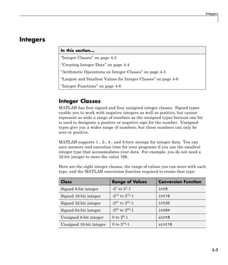
Integers . . . . . . . . . . . . . . . . . . . . . . . . . . . . . . . . . . . . . . . . . . 4-3
Integer Classes . . . . . . . . . . . . . . . . . . . . . . . . . . . . . . . . . . . 4-3
viii Contents](https://image.slidesharecdn.com/matlabprog-220902050722-ff974cdf/85/matlab_prog-pdf-8-320.jpg)

![1 Syntax Basics
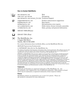
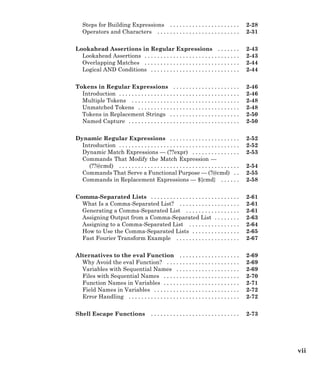
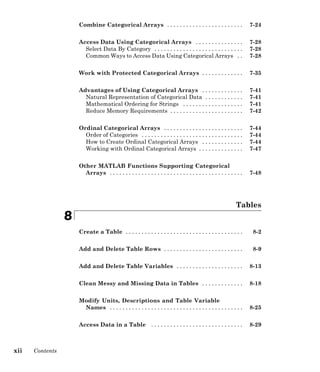
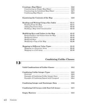
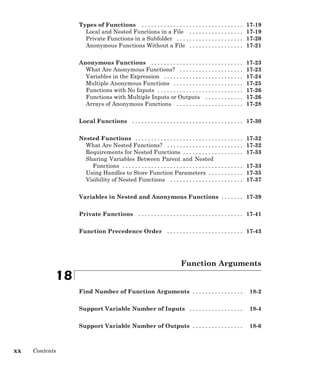
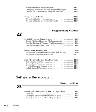
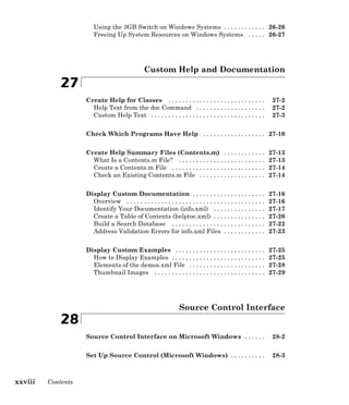
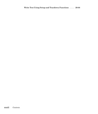
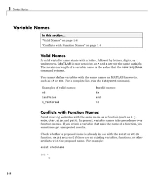
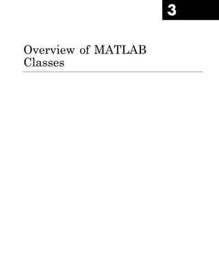
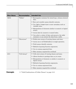
Create Variables
This example shows several ways to assign a value to a variable.
x = 5.71;
A = [1 2 3; 4 5 6; 7 8 9];
I = besseli(x,A);
You do not have to declare variables before assigning values.
If you do not end an assignment statement with a semicolon (;), MATLAB®
displays the result in the Command Window. For example,
x = 5.71
displays
x =
5.7100
If you do not explicitly assign the output of a command to a variable, MATLAB
generally assigns the result to the reserved word ans. For example,
5.71
returns
ans =
5.7100
The value of ans changes with every command that returns an output value
that is not assigned to a variable.
1-2](https://image.slidesharecdn.com/matlabprog-220902050722-ff974cdf/85/matlab_prog-pdf-36-320.jpg)
![Create Numeric Arrays
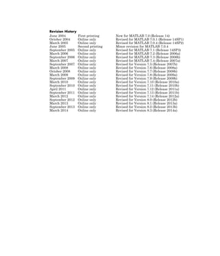
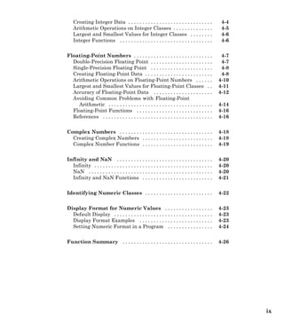
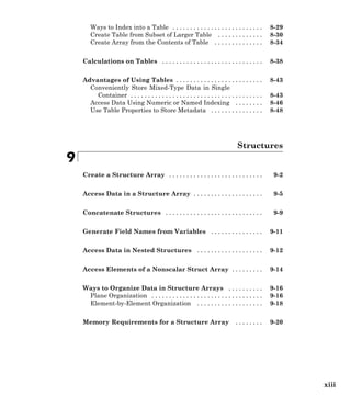
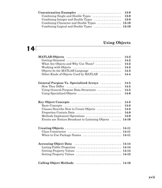
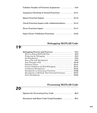
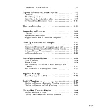
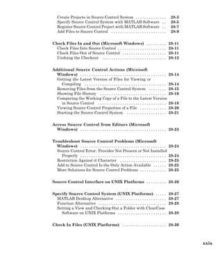
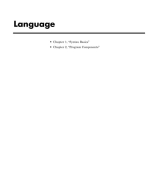
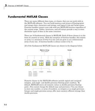
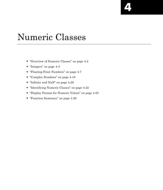
Create Numeric Arrays
This example shows how to create a numeric variable. In the MATLAB
computing environment, all variables are arrays, and by default, numeric
variables are of type double (that is, double-precision values). For example,
create a scalar value.
A = 100;
Because scalar values are single element, 1-by-1 arrays,
whos A
returns
Name Size Bytes Class Attributes
A 1x1 8 double
To create a matrix (a two-dimensional, rectangular array of numbers), you
can use the [] operator.
B = [12, 62, 93, -8, 22; 16, 2, 87, 43, 91; -4, 17, -72, 95, 6]
When using this operator, separate columns with a comma or space, and
separate rows with a semicolon. All rows must have the same number of
elements. In this example, B is a 3-by-5 matrix (that is, B has three rows
and five columns).
B =
12 62 93 -8 22
16 2 87 43 91
-4 17 -72 95 6
A matrix with only one row or column (that is, a 1-by-n or n-by-1 array) is
a vector, such as
C = [1, 2, 3]
or
D = [10; 20; 30]
1-3](https://image.slidesharecdn.com/matlabprog-220902050722-ff974cdf/85/matlab_prog-pdf-37-320.jpg)
![Continue Long Statements on Multiple Lines
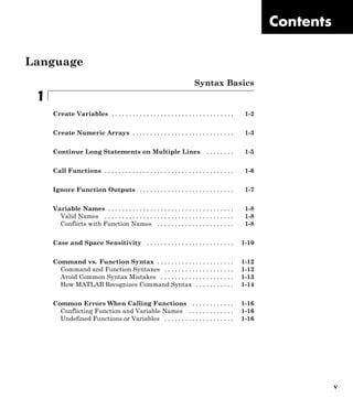
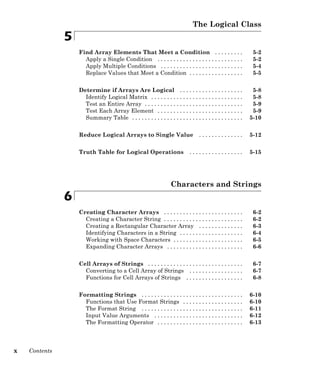
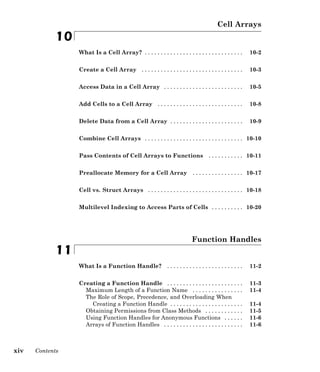
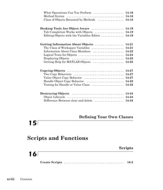
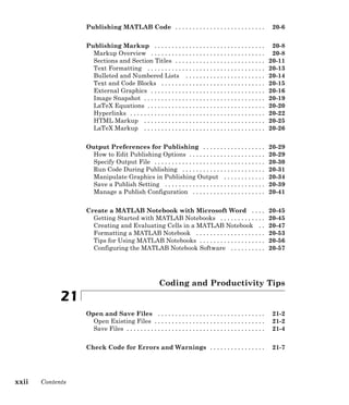
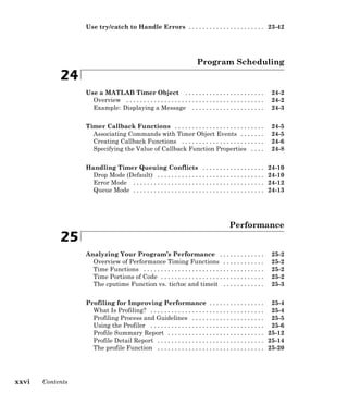
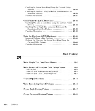
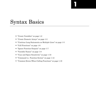
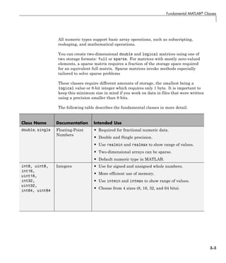
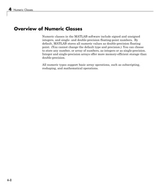
Continue Long Statements on Multiple Lines
This example shows how to continue a statement to the next line using
ellipses (...).
s = 1 - 1/2 + 1/3 - 1/4 + 1/5 ...
- 1/6 + 1/7 - 1/8 + 1/9;
Build a long character string by concatenating shorter strings together:
mystring = ['Accelerating the pace of ' ...
'engineering and science'];
The start and end quotation marks for a string must appear on the same
line. For example, this code returns an error, because each line contains only
one quotation mark:
mystring = 'Accelerating the pace of ...
engineering and science'
An ellipses outside a quoted string is equivalent to a space. For example,
x = [1.23...
4.56];
is the same as
x = [1.23 4.56];
1-5](https://image.slidesharecdn.com/matlabprog-220902050722-ff974cdf/85/matlab_prog-pdf-39-320.jpg)
![1 Syntax Basics
Call Functions
These examples show how to call a MATLAB function. To run the examples,
you must first create numeric arrays A and B, such as:
A = [1 3 5];
B = [10 6 4];
Enclose inputs to functions in parentheses:
max(A)
Separate multiple inputs with commas:
max(A,B)
Store output from a function by assigning it to a variable:
maxA = max(A)
Enclose multiple outputs in square brackets:
[maxA, location] = max(A)
Call a function that does not require any inputs, and does not return any
outputs, by typing only the function name:
clc
Enclose text string inputs in single quotation marks:
disp('hello world')
Related
Examples
• “Ignore Function Outputs” on page 1-7
1-6](https://image.slidesharecdn.com/matlabprog-220902050722-ff974cdf/85/matlab_prog-pdf-40-320.jpg)
![Ignore Function Outputs
Ignore Function Outputs
This example shows how to request specific outputs from a function.
Request all three possible outputs from the fileparts function.
helpFile = which('help');
[helpPath,name,ext] = fileparts(helpFile);
The current workspace now contains three variables from fileparts:
helpPath, name, and ext. In this case, the variables are small. However,
some functions return results that use much more memory. If you do not need
those variables, they waste space on your system.
Request only the first output, ignoring the second and third.
helpPath = fileparts(helpFile);
For any function, you can request only the first outputs (where is less
than or equal to the number of possible outputs) and ignore any remaining
outputs. If you request more than one output, enclose the variable names in
square brackets, [].
Ignore the first output using a tilde (~).
[~,name,ext] = fileparts(helpFile);
You can ignore any number of function outputs, in any position in the
argument list. Separate consecutive tildes with a comma, such as
[~,~,ext] = fileparts(helpFile);
1-7](https://image.slidesharecdn.com/matlabprog-220902050722-ff974cdf/85/matlab_prog-pdf-41-320.jpg)
![1 Syntax Basics
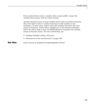
Case and Space Sensitivity
MATLAB code is sensitive to casing, and insensitive to blank spaces except
when defining arrays.
Uppercase and Lowercase
In MATLAB code, use an exact match with regard to case for variables, files,
and functions. For example, if you have a variable, a, you cannot refer to
that variable as A. It is a best practice to use lowercase only when naming
functions. This is especially useful when you use both Microsoft® Windows®
and UNIX®1
platforms because their file systems behave differently with
regard to case.
When you use the help function, the help displays some function names in all
uppercase, for example, PLOT, solely to distinguish the function name from the
rest of the text. Some functions for interfacing to Oracle® Java® software do
use mixed case and the command-line help and the documentation accurately
reflect that.
Spaces
Blank spaces around operators such as -, :, and ( ), are optional, but they
can improve readability. For example, MATLAB interprets the following
statements the same way.
y = sin (3 * pi) / 2
y=sin(3*pi)/2
However, blank spaces act as delimiters in horizontal concatenation. When
defining row vectors, you can use spaces and commas interchangeably to
separate elements:
A = [1, 0 2, 3 3]
A =
1 0 2 3 3
1. UNIX is a registered trademark of The Open Group in the United States and other
countries.
1-10](https://image.slidesharecdn.com/matlabprog-220902050722-ff974cdf/85/matlab_prog-pdf-44-320.jpg)
![Case and Space Sensitivity
Because of this flexibility, check to ensure that MATLAB stores the correct
values. For example, the statement [1 sin (pi) 3] produces a much
different result than [1 sin(pi) 3] does.
[1 sin (pi) 3]
Error using sin
Not enough input arguments.
[1 sin(pi) 3]
ans =
1.0000 0.0000 3.0000
1-11](https://image.slidesharecdn.com/matlabprog-220902050722-ff974cdf/85/matlab_prog-pdf-45-320.jpg)
![1 Syntax Basics
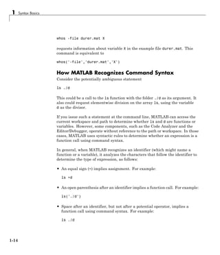
Command vs. Function Syntax
In this section...
“Command and Function Syntaxes” on page 1-12
“Avoid Common Syntax Mistakes” on page 1-13
“How MATLAB Recognizes Command Syntax” on page 1-14
Command and Function Syntaxes
In MATLAB, these statements are equivalent:
load durer.mat % Command syntax
load('durer.mat') % Function syntax
This equivalence is sometimes referred to as command-function duality.
All functions support this standard function syntax:
[output1, ..., outputM] = functionName(input1, ..., inputN)
If you do not require any outputs from the function, and all of the inputs
are literal strings (that is, text enclosed in single quotation marks), you can
use this simpler command syntax:
functionName input1 ... inputN
With command syntax, you separate inputs with spaces rather than commas,
and do not enclose input arguments in parentheses. Because all inputs are
literal strings, single quotation marks are optional, unless the input string
contains spaces. For example:
disp 'hello world'
When a function input is a variable, you must use function syntax to pass the
value to the function. Command syntax always passes inputs as literal text
and cannot pass variable values. For example, create a variable and call the
disp function with function syntax to pass the value of the variable:
A = 123;
disp(A)
1-12](https://image.slidesharecdn.com/matlabprog-220902050722-ff974cdf/85/matlab_prog-pdf-46-320.jpg)
![Command vs. Function Syntax
This code returns the expected result,
123
You cannot use command syntax to pass the value of A, because this call
disp A
is equivalent to
disp('A')
and returns
A
Avoid Common Syntax Mistakes
Suppose that your workspace contains these variables:
filename = 'accounts.txt';
A = int8(1:8);
B = A;
The following table illustrates common misapplications of command syntax.
This Command... Is Equivalent to... Correct Syntax for Passing
Value
open filename open('filename') open(filename)
isequal A B isequal('A','B') isequal(A,B)
strcmp class(A) int8 strcmp('class(A)','int8') strcmp(class(A),'int8')
cd matlabroot cd('matlabroot') cd(matlabroot)
isnumeric 500 isnumeric('500') isnumeric(500)
round 3.499 round('3.499'), same as
round([51 46 52 57 57])
round(3.499)
Passing Variable Names
Some functions expect literal strings for variable names, such as save, load,
clear, and whos. For example,
1-13](https://image.slidesharecdn.com/matlabprog-220902050722-ff974cdf/85/matlab_prog-pdf-47-320.jpg)


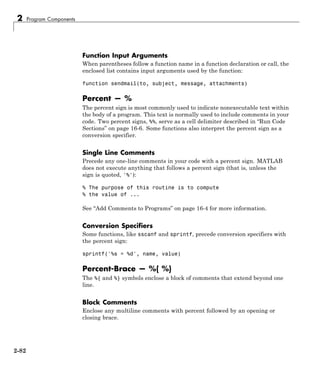
![2 Program Components
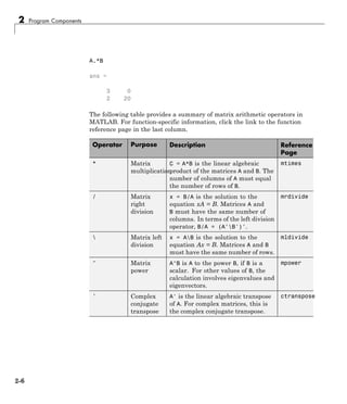
Array vs. Matrix Operations
In this section...
“Introduction” on page 2-2
“Array Operations” on page 2-2
“Matrix Operations” on page 2-4
Introduction
MATLAB has two different types of arithmetic operations: array operations
and matrix operations. You can use these arithmetic operations to perform
numeric computations, for example, adding two numbers, raising the
elements of an array to a given power, or multiplying two matrices.
Matrix operations follow the rules of linear algebra. By contrast,
array operations execute element by element operations and support
multidimensional arrays. The period character (.) distinguishes the array
operations from the matrix operations. However, since the matrix and array
operations are the same for addition and subtraction, the character pairs
.+ and .- are unnecessary.
Array Operations
Array operations work on corresponding elements of arrays with equal
dimensions. For vectors, matrices, and multidimensional arrays, both
operands must be the same size. Each element in the first input gets matched
up with a similarly located element from the second input. If the inputs are
different sizes, MATLAB cannot match the elements one-to-one.
As a simple example, you can add two vectors with the same length.
A = [1 1 1]
A =
1 1 1
B = 1:3
2-2](https://image.slidesharecdn.com/matlabprog-220902050722-ff974cdf/85/matlab_prog-pdf-58-320.jpg)
![Array vs. Matrix Operations
B =
1 2 3
A+B
ans =
2 3 4
If the vectors are not the same size you get an error.
B = 1:4
B =
1 2 3 4
A+B
Error using +
Matrix dimensions must agree.
If one operand is a scalar and the other is not, then MATLAB applies the
scalar to every element of the other operand. This property is known as scalar
expansion because the scalar expands into an array of the same size as the
other input, then the operation executes as it normally does with two arrays.
For example, the element-wise product of a scalar and a matrix uses scalar
expansion.
A = [1 0 2;3 1 4]
A =
1 0 2
3 1 4
3.*A
2-3](https://image.slidesharecdn.com/matlabprog-220902050722-ff974cdf/85/matlab_prog-pdf-59-320.jpg)
![Array vs. Matrix Operations
the matrix operators generally calculate different answers than their array
operator counterparts.
For example, if you use the matrix right division operator, /, to divide two
matrices, the matrices must have the same number of columns. But if you
use the matrix multiplication operator, *, to multiply two matrices, then
the matrices must have a common inner dimension. That is, the number
of columns in the first input must be equal to the number of rows in the
second input. The matrix multiplication operator calculates the product of
two matrices with the formula,
C i j A i k B k j
k
n
( , ) ( , ) ( , ).
1
To see this, you can calculate the product of two matrices.
A = [1 3;2 4]
A =
1 3
2 4
B = [3 0;1 5]
B =
3 0
1 5
A*B
ans =
6 15
10 20
The previous matrix product is not equal to the following element-wise
product.
2-5](https://image.slidesharecdn.com/matlabprog-220902050722-ff974cdf/85/matlab_prog-pdf-61-320.jpg)
![Relational Operators
Relational Operators
Relational operators compare operands quantitatively, using operators like
“less than” and “not equal to.” The following table provides a summary. For
more information, see the relational operators reference page.
Operator Description
< Less than
<= Less than or equal to
> Greater than
>= Greater than or equal to
== Equal to
~= Not equal to
Relational Operators and Arrays
The MATLAB relational operators compare corresponding elements
of arrays with equal dimensions. Relational operators always operate
element-by-element. In this example, the resulting matrix shows where an
element of A is equal to the corresponding element of B.
A = [2 7 6;9 0 5;3 0.5 6];
B = [8 7 0;3 2 5;4 -1 7];
A == B
ans =
0 1 0
0 0 1
0 0 0
For vectors and rectangular arrays, both operands must be the same size
unless one is a scalar. For the case where one operand is a scalar and the
other is not, MATLAB tests the scalar against every element of the other
operand. Locations where the specified relation is true receive logical 1.
Locations where the relation is false receive logical 0.
2-7](https://image.slidesharecdn.com/matlabprog-220902050722-ff974cdf/85/matlab_prog-pdf-63-320.jpg)
![2 Program Components
Relational Operators and Empty Arrays
The relational operators work with arrays for which any dimension has size
zero, as long as both arrays are the same size or one is a scalar. However,
expressions such as
A == []
return an error if A is not 0-by-0 or 1-by-1. This behavior is consistent with
that of all other binary operators, such as +, -, >, <, &, |, etc.
To test for empty arrays, use the function
isempty(A)
2-8](https://image.slidesharecdn.com/matlabprog-220902050722-ff974cdf/85/matlab_prog-pdf-64-320.jpg)
![2 Program Components
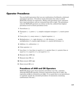
The same precedence rule holds true for the && and || operators.
Overriding Default Precedence
The default precedence can be overridden using parentheses, as shown in
this example:
A = [3 9 5];
B = [2 1 5];
C = A./B.^2
C =
0.7500 9.0000 0.2000
C = (A./B).^2
C =
2.2500 81.0000 1.0000
2-10](https://image.slidesharecdn.com/matlabprog-220902050722-ff974cdf/85/matlab_prog-pdf-66-320.jpg)
![2 Program Components
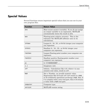
Here are some examples that use these values in MATLAB expressions.
x = 2 * pi
x =
6.2832
A = [3+2i 7-8i]
A =
3.0000 + 2.0000i 7.0000 - 8.0000i
tol = 3 * eps
tol =
6.6613e-016
intmax('uint64')
ans =
18446744073709551615
2-12](https://image.slidesharecdn.com/matlabprog-220902050722-ff974cdf/85/matlab_prog-pdf-68-320.jpg)
![Conditional Statements
Conditional Statements
Conditional statements enable you to select at run time which block of code to
execute. The simplest conditional statement is an if statement. For example:
% Generate a random number
a = randi(100, 1);
% If it is even, divide by 2
if rem(a, 2) == 0
disp('a is even')
b = a/2;
end
if statements can include alternate choices, using the optional keywords
elseif or else. For example:
a = randi(100, 1);
if a < 30
disp('small')
elseif a < 80
disp('medium')
else
disp('large')
end
Alternatively, when you want to test for equality against a set of known
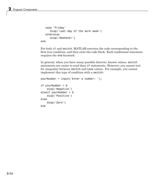
values, use a switch statement. For example:
[dayNum, dayString] = weekday(date, 'long', 'en_US');
switch dayString
case 'Monday'
disp('Start of the work week')
case 'Tuesday'
disp('Day 2')
case 'Wednesday'
disp('Day 3')
case 'Thursday'
disp('Day 4')
2-13](https://image.slidesharecdn.com/matlabprog-220902050722-ff974cdf/85/matlab_prog-pdf-69-320.jpg)
![Represent Dates and Times in MATLAB®
Represent Dates and Times in MATLAB
MATLAB represents date and time information in any of three formats:
• Date String — A character string.
Example: Thursday, August 23, 2012 9:45:44.946 AM
• Date Vector — A 1-by-6 numeric vector containing the year, month, day,
hour, minute, and second.
Example: [2012 8 23 9 45 44.946]
• Serial Date Number — A single number equal to the number of days since
January 0, 0000.
Example: 7.3510e+005
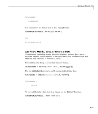
You can use any of these formats. If you work with more than one date and
time format, you can convert from one format to another using the datestr,
datevec, and datenum functions.
Date Strings
A date string is a character string composed of fields related to a specific date
and/or time. There are several ways to represent dates and times in character
string format. For example, all of the following are date strings for August 23,
2010 at 04:35:42 PM:
'23-Aug-2010 04:35:06 PM'
'Wednesday, August 23'
'08/23/10 16:35'
'Aug 23 16:35:42.946'
You can represent time in a date string using either a 12-hour or 24-hour
system.
When you create a date string, include any characters you might need to
separate the fields, such as the hyphen, space, and colon used here:
d = '23-Aug-2010 16:35:42'
2-17](https://image.slidesharecdn.com/matlabprog-220902050722-ff974cdf/85/matlab_prog-pdf-73-320.jpg)
![2 Program Components
Date Vectors
A date vector is a 1-by-6 matrix of double-precision numbers. Elements of a
date vector are integer valued, with the exception of the seconds element,
which can be fractional. A date vector is arranged in the following order:
year month day hour minute second
The following date vector represents 10:45:07 AM on October 24, 2012:
[2012 10 24 10 45 07]
Date vectors must follow these guidelines:
• Date vectors have no separate field in which to specify milliseconds.
However, the seconds field has a fractional part and accurately keeps
the milliseconds field.
• Time values are expressed in 24-hour notation. There is no AM or PM
setting.
Serial Date Numbers
A serial date number represents a calendar date as the number of days that
has passed since a fixed base date. In MATLAB, serial date number 1 is
January 1, 0000.
MATLAB also uses serial time to represent fractions of days beginning
at midnight; for example, 6 p.m. equals 0.75 serial days. So the string
'31-Oct-2003, 6:00 PM' in MATLAB is date number 731885.75.
If you pass date vectors or date strings to a MATLAB function that accepts
such inputs, MATLAB first converts the input to serial date numbers. If you
are working with a large number of dates or doing extensive calculations with
dates, use serial date numbers for better performance.
2-18](https://image.slidesharecdn.com/matlabprog-220902050722-ff974cdf/85/matlab_prog-pdf-74-320.jpg)
![Carryover in Date Vectors and Strings
Carryover in Date Vectors and Strings
If an element falls outside the conventional range, MATLAB adjusts both that
date vector element and the previous element. For example, if the minutes
element is 70, MATLAB adjusts the hours element by 1 and sets the minutes
element to 10. If the minutes element is -15, then MATLAB decreases the
hours element by 1 and sets the minutes element to 45. Month values are an
exception. MATLAB sets month values less than 1 to 1.
In the following example, the month element has a value of 22. MATLAB
increments the year value to 2010 and sets the month to October.
datestr([2009 22 03 00 00 00])
ans =
03-Oct-2010
The carrying forward of values also applies to time and day values in date
strings. For example, October 3, 2010 and September 33, 2010 are interpreted
to be the same date, and correspond to the same serial date number.
datenum('03-Oct-2010')
ans =
734414
datenum('33-Sep-2010')
ans =
734414
The following example takes the input month (07, or July), finds the last day
of the previous month (June 30), and subtracts the number of days in the field
specifier (5 days) from that date to yield a return date of June 25, 2010.
datestr([2010 07 -05 00 00 00])
ans =
25-Jun-2010
2-23](https://image.slidesharecdn.com/matlabprog-220902050722-ff974cdf/85/matlab_prog-pdf-79-320.jpg)
![2 Program Components
Troubleshooting: Converting Date Vector Returns
Unexpected Output
Because a date vector is a 1-by-6 vector of numbers, datestr might interpret
your input date vectors as vectors of serial date numbers, or vice versa, and
return unexpected output.
Consider a date vector that includes the year 3000. This year is outside the
range of years that datestr interprets as elements of date vectors. Therefore,
the input is interpreted as a 1-by-6 vector of serial date numbers:
datestr([3000 11 05 10 32 56])
ans =
18-Mar-0008
11-Jan-0000
05-Jan-0000
10-Jan-0000
01-Feb-0000
25-Feb-0000
Here datestr interprets 3000 as a serial date number, and converts it to the
date string '18-Mar-0008'. Also, datestr converts the next five elements to
date strings.
When converting such a date vector to a string, first convert it to a serial date
number using datenum. Then, convert the date number to a string using
datestr:
dn = datenum([3000 11 05 10 32 56]);
ds = datestr(dn)
ds =
05-Nov-3000 10:32:56
When converting dates to strings, datestr interprets input as either date
vectors or serial date numbers using a heuristic rule. Consider an m-by-6
matrix. datestr interprets the matrix as m date vectors when:
2-24](https://image.slidesharecdn.com/matlabprog-220902050722-ff974cdf/85/matlab_prog-pdf-80-320.jpg)
![Troubleshooting: Converting Date Vector Returns Unexpected Output
• The first five columns contain integers.
• The absolute value of the sum of each row is in the range 1500–2500.
If either condition is false, for any row, then datestr interprets the m-by-6
matrix as m-by-6 serial date numbers.
Usually, dates with years in the range 1700–2300 are interpreted as date
vectors. However, datestr might interpret rows with month, day, hour,
minute, or second values outside their normal ranges as serial date numbers.
For example, datestr correctly interprets the following date vector for the
year 2014:
datestr([2014 06 21 10 51 00])
ans =
21-Jun-2014 10:51:00
But given a day value outside the typical range (1–31), datestr returns a
date for each element of the vector:
datestr([2014 06 2110 10 51 00])
ans =
06-Jul-0005
06-Jan-0000
10-Oct-0005
10-Jan-0000
20-Feb-0000
00-Jan-0000
When you have a matrix of date vectors that datestr might interpret
incorrectly as serial date numbers, first convert the matrix to serial date
numbers using datenum. Then, use datestr to convert the date numbers.
When you have a matrix of serial date numbers that datestr might interpret
as date vectors, first convert the matrix to a column vector. Then, use datestr
to convert the column vector.
2-25](https://image.slidesharecdn.com/matlabprog-220902050722-ff974cdf/85/matlab_prog-pdf-81-320.jpg)
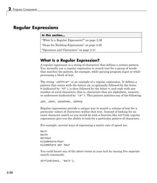
![Regular Expressions
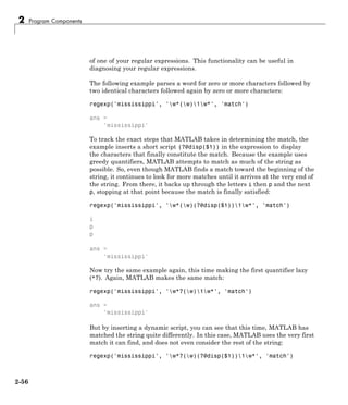
strfind(text, 'km/hour');
% etc.
To be more efficient, however, you can build a single phrase that applies to
all of these search strings:
Translate this phrase it into a regular expression (to be explained later in
this section) and you have:
pattern = 'k(ilo)?m(eters)?(/|spers)h(r|our)?';
Now locate one or more of the strings using just a single command:
text = ['The high-speed train traveled at 250 ', ...
'kilometers per hour alongside the automobile ', ...
'travelling at 120 km/h.'];
regexp(text, pattern, 'match')
ans =
'kilometers per hour' 'km/h'
There are four MATLAB functions that support searching and replacing
characters using regular expressions. The first three are similar in the input
values they accept and the output values they return. For details, click the
links to the function reference pages.
Function Description
regexp Match regular expression.
regexpi Match regular expression, ignoring case.
2-27](https://image.slidesharecdn.com/matlabprog-220902050722-ff974cdf/85/matlab_prog-pdf-83-320.jpg)
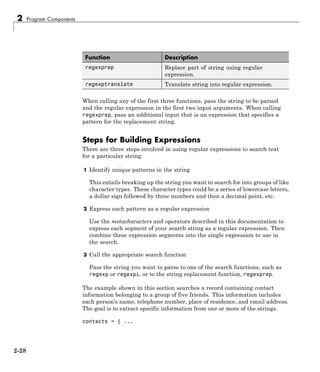
![2 Program Components
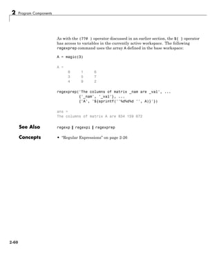
Step 2 — Express Each Pattern as a Regular Expression
In this step, you translate the general formats derived in Step 1 into segments
of a regular expression. You then add these segments together to form the
entire expression.
The table below shows the generalized format descriptions of each character
pattern in the left-most column. (This was carried forward from the right
column of the table in Step 1.) The second column shows the operators or
metacharacters that represent the character pattern.
Description of each segment Pattern
One or more lowercase letters and underscores [a-z_]+
@ sign @
One or more lowercase letters, no underscores [a-z]+
Dot (period) character .
com or net (com|net)
Assembling these patterns into one string gives you the complete expression:
email = '[a-z_]+@[a-z]+.(com|net)';
Step 3 — Call the Appropriate Search Function
In this step, you use the regular expression derived in Step 2 to match an
email address for one of the friends in the group. Use the regexp function
to perform the search.
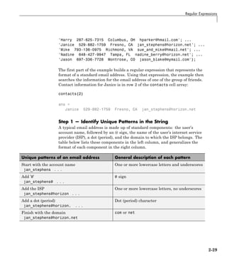
Here is the list of contact information shown earlier in this section. Each
person’s record occupies a row of the contacts cell array:
contacts = { ...
'Harry 287-625-7315 Columbus, OH hparker@hmail.com'; ...
'Janice 529-882-1759 Fresno, CA jan_stephens@horizon.net'; ...
'Mike 793-136-0975 Richmond, VA sue_and_mike@hmail.net'; ...
'Nadine 648-427-9947 Tampa, FL nadine_berry@horizon.net'; ...
'Jason 697-336-7728 Montrose, CO jason_blake@mymail.com'};
2-30](https://image.slidesharecdn.com/matlabprog-220902050722-ff974cdf/85/matlab_prog-pdf-86-320.jpg)
![Regular Expressions
This is the regular expression that represents an email address, as derived
in Step 2:
email = '[a-z_]+@[a-z]+.(com|net)';
Call the regexp function, passing row 2 of the contacts cell array and the
email regular expression. This returns the email address for Janice.
regexp(contacts{2}, email, 'match')
ans =
'jan_stephens@horizon.net'
MATLAB parses a string from left to right, “consuming” the string as it goes.
If matching characters are found, regexp records the location and resumes
parsing the string, starting just after the end of the most recent match.
Make the same call, but this time for the fifth person in the list:
regexp(contacts{5}, email, 'match')
ans =
'jason_blake@mymail.com'
You can also search for the email address of everyone in the list by using the
entire cell array for the input string argument:
regexp(contacts, email, 'match');
Operators and Characters
Regular expressions can contain characters, metacharacters, operators,
tokens, and flags that specify patterns to match, as described in these sections:
• “Metacharacters” on page 2-32
• “Character Representation” on page 2-33
• “Quantifiers” on page 2-34
• “Grouping Operators” on page 2-35
• “Anchors” on page 2-36
• “Lookaround Assertions” on page 2-36
2-31](https://image.slidesharecdn.com/matlabprog-220902050722-ff974cdf/85/matlab_prog-pdf-87-320.jpg)
![2 Program Components
• “Logical and Conditional Operators” on page 2-37
• “Token Operators” on page 2-38
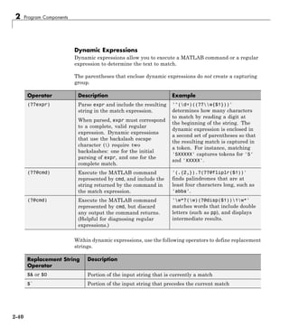
• “Dynamic Expressions” on page 2-40
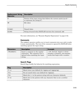
• “Comments” on page 2-41
• “Search Flags” on page 2-41
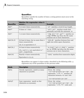
Metacharacters
Metacharacters represent letters, letter ranges, digits, and space characters.
Use them to construct a generalized pattern of characters.
Metacharacter Description Example
. Any single character, including
white space
'..ain' matches sequences of five
consecutive characters that end with
'ain'.
[c1
c2
c3
] Any character contained within the
brackets. The following characters
are treated literally: $ | . * +
? and - when not used to indicate
a range.
'[rp.]ain' matches 'rain' or 'pain'
or `.ain'.
[^c1
c2
c3
] Any character not contained
within the brackets. The following
characters are treated literally: $
| . * + ? and - when not used
to indicate a range.
'[^*rp]ain' matches all four-letter
sequences that end in 'ain', except
'rain' and 'pain' and `*ain'. For
example, it matches 'gain', 'lain', or
'vain'.
[c1-c2] Any character in the range of c1
through c2
'[A-G]' matches a single character in
the range of A through G.
w Any alphabetic, numeric, or
underscore character. For English
character sets, w is equivalent to
[a-zA-Z_0-9]
'w*' identifies a word.
2-32](https://image.slidesharecdn.com/matlabprog-220902050722-ff974cdf/85/matlab_prog-pdf-88-320.jpg)
![Regular Expressions
Metacharacter Description Example
W Any character that is not
alphabetic, numeric, or underscore.
For English character sets, W is
equivalent to [^a-zA-Z_0-9]
'W*' identifies a substring that is not
a word.
s Any white-space character;
equivalent to [ fnrtv]
'w*ns' matches words that end with
the letter n, followed by a white-space
character.
S Any non-white-space character;
equivalent to [^ fnrtv]
'dS' matches a numeric digit followed
by any non-white-space character.
d Any numeric digit; equivalent to
[0-9]
'd*' matches any number of
consecutive digits.
D Any nondigit character; equivalent
to [^0-9]
'w*D>' matches words that do not
end with a numeric digit.
oN or o{N} Character of octal value N 'o{40}' matches the space character,
defined by octal 40.
xN or x{N} Character of hexadecimal value N 'x2C' matches the comma character,
defined by hex 2C.
Character Representation
Operator Description
a Alarm (beep)
b Backspace
f Form feed
n New line
r Carriage return
t Horizontal tab
v Vertical tab
char Any character with special meaning in regular expressions that you want to
match literally (for example, use to match a single backslash)
2-33](https://image.slidesharecdn.com/matlabprog-220902050722-ff974cdf/85/matlab_prog-pdf-89-320.jpg)
![Regular Expressions
Mode Description Example
match at the first occurrence of the
closing bracket (>):
'<tr>' '<td>' '</td>'
exprq+ Possessive expression: match as much
as possible, but do not rescan any
portions of the string.
Given the string
'<tr><td><p>text</p></td>', the
expression '</?t.*+>' does not return
any matches, because the closing
bracket is captured using .*, and is
not rescanned.
Grouping Operators
Grouping operators allow you to capture tokens, apply one operator to
multiple elements, or disable backtracking in a specific group.
Grouping
Operator Description Example
(expr) Group elements of the expression and
capture tokens.
'Joh?ns(w*)' captures a token that
contains the last name of any person
with the first name John or Jon.
(?:expr) Group, but do not capture tokens. '(?:[aeiou][^aeiou]){2}' matches
two consecutive patterns of a vowel
followed by a nonvowel, such as
'anon'.
Without grouping,
'[aeiou][^aeiou]{2}'matches
a vowel followed by two nonvowels.
2-35](https://image.slidesharecdn.com/matlabprog-220902050722-ff974cdf/85/matlab_prog-pdf-91-320.jpg)
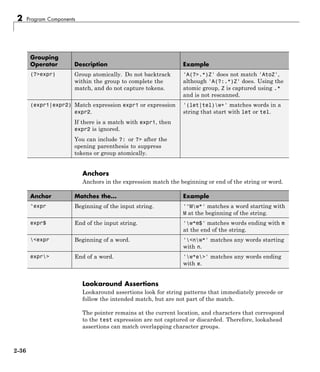
![Regular Expressions
Lookaround
Assertion Description Example
expr(?=test) Look ahead for characters that match
test.
'w*(?=ing)' matches strings that
are followed by ing, such as 'Fly' and
'fall' in the input string 'Flying,
not falling.'
expr(?!test) Look ahead for characters that do not
match test.
'i(?!ng)' matches instances of the
letter i that are not followed by ng.
(?<=test)expr Look behind for characters that
match test..
'(?<=re)w*' matches strings that
follow 're', such as 'new', 'use', and
'cycle' in the input string 'renew,
reuse, recycle'
(?<!test)expr Look behind for characters that do
not match test.
'(?<!d)(d)(?!d)' matches
single-digit numbers (digits that do
not precede or follow other digits).
If you specify a lookahead assertion before an expression, the operation is
equivalent to a logical AND.
Operation Description Example
(?=test)expr Match both test and expr. '(?=[a-z])[^aeiou]' matches
consonants.
(?!test)expr Match expr and do not match test. '(?![aeiou])[a-z]' matches
consonants.
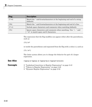
For more information, see “Lookahead Assertions in Regular Expressions”
on page 2-43.
Logical and Conditional Operators
Logical and conditional operators allow you to test the state of a given
condition, and then use the outcome to determine which string, if any, to
match next. These operators support logical OR and if or if/else conditions.
(For AND conditions, see “Lookaround Assertions” on page 2-36.)
2-37](https://image.slidesharecdn.com/matlabprog-220902050722-ff974cdf/85/matlab_prog-pdf-93-320.jpg)
![2 Program Components
Conditions can be tokens, lookaround assertions, or dynamic expressions of
the form (?@cmd). Dynamic expressions must return a logical or numeric
value.
Conditional Operator Description Example
expr1|expr2 Match expression expr1 or
expression expr2.
If there is a match with expr1,
then expr2 is ignored.
'(let|tel)w+' matches words
in a string that start with let or
tel.
(?(cond)expr) If condition cond is true, then
match expr.
'(?(?@ispc)[A-Z]:)' matches
a drive name, such as C:, when
run on a Windows system.
(?(cond)expr1|expr2) If condition cond is true, then
match expr1. Otherwise, match
expr2.
'Mr(s?)..*?(?(1)her|his)
w*' matches strings that include
her when the string begins with
Mrs, or that include his when the
string begins with Mr.
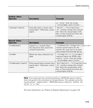
Token Operators
Tokens are portions of the matched text that you define by enclosing part
of the regular expression in parentheses. You can refer to a token by its
sequence in the string (an ordinal token), or assign names to tokens for easier
code maintenance and readable output.
Ordinal Token
Operator Description Example
(expr) Capture in a token the characters
that match the enclosed
expression.
'Joh?ns(w*)' captures a token
that contains the last name of any
person with the first name John
or Jon.
N Match the Nth token. '<(w+).*>.*</1>' captures
tokens for HTML tags, such
2-38](https://image.slidesharecdn.com/matlabprog-220902050722-ff974cdf/85/matlab_prog-pdf-94-320.jpg)
![Lookahead Assertions in Regular Expressions
Lookahead Assertions in Regular Expressions
In this section...
“Lookahead Assertions” on page 2-43
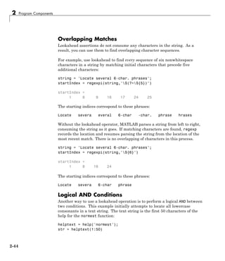
“Overlapping Matches” on page 2-44
“Logical AND Conditions” on page 2-44
Lookahead Assertions
There are two types of lookaround assertions for regular expressions:
lookahead and lookbehind. In both cases, the assertion is a condition that
must be satisfied to return a match to the expression.
A lookahead assertion has the form (?=test) and can appear anywhere in a
regular expression. MATLAB looks ahead of the current location in the string
for the test condition. If MATLAB matches the test condition, it continues
processing the rest of the expression to find a match.
For example, look ahead in a path string to find the name of the folder that
contains a program file (in this case, fileread.m).
str = which('fileread')
str =
matlabroottoolboxmatlabiofunfileread.m
regexp(str,'w+(?=w+.[mp])','match')
ans =
'iofun'
The match expression, w+, searches for one or more alphanumeric or
underscore characters. Each time regexp finds a string that matches this
condition, it looks ahead for a backslash (specified with two backslashes, ),
followed by a file name (w+) with an .m or .p extension (.[mp]). The regexp
function returns the match that satisfies the lookahead condition, which is
the folder name iofun.
2-43](https://image.slidesharecdn.com/matlabprog-220902050722-ff974cdf/85/matlab_prog-pdf-99-320.jpg)
![Lookahead Assertions in Regular Expressions
str =
NORMEST Estimate the matrix 2-norm.
NORMEST(S
Merely searching for non-vowels ([^aeiou]) does not return the expected
answer, as the output includes capital letters, space characters, and
punctuation:
c = regexp(str,'[^aeiou]','match')
c =
Columns 1 through 14
' ' 'N' 'O' 'R' 'M' 'E' 'S' 'T' ' '
'E' 's' 't' 'm' 't'
...
Try this again, using a lookahead operator to create the following AND
condition:
(lowercase letter) AND (not a vowel)
This time, the result is correct:
c = regexp(str,'(?=[a-z])[^aeiou]','match')
c =
's' 't' 'm ' 't' 't' 'h' 'm' 't' 'r' 'x'
'n' 'r' 'm'
Note that when using a lookahead operator to perform an AND, you need to
place the match expression expr after the test expression test:
(?=test)expr or (?!test)expr
See Also regexp | regexpi | regexprep
Concepts • “Regular Expressions” on page 2-26
2-45](https://image.slidesharecdn.com/matlabprog-220902050722-ff974cdf/85/matlab_prog-pdf-101-320.jpg)
![2 Program Components
Tokens in Regular Expressions
In this section...
“Introduction” on page 2-46
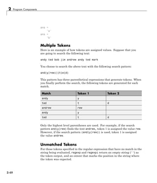
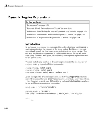
“Multiple Tokens” on page 2-48
“Unmatched Tokens” on page 2-48
“Tokens in Replacement Strings” on page 2-50
“Named Capture” on page 2-50
Introduction
Parentheses used in a regular expression not only group elements of that
expression together, but also designate any matches found for that group as
tokens. You can use tokens to match other parts of the same string. One
advantage of using tokens is that they remember what they matched, so you
can recall and reuse matched text in the process of searching or replacing.
Each token in the expression is assigned a number, starting from 1, going
from left to right. To make a reference to a token later in the expression,
refer to it using a backslash followed by the token number. For example,
when referencing a token generated by the third set of parentheses in the
expression, use 3.
As a simple example, if you wanted to search for identical sequential letters
in a string, you could capture the first letter as a token and then search for a
matching character immediately afterwards. In the expression shown below,
the (S) phrase creates a token whenever regexp matches any nonwhitespace
character in the string. The second part of the expression, '1', looks for a
second instance of the same character immediately following the first:
poestr = ['While I nodded, nearly napping, ' ...
'suddenly there came a tapping,'];
[mat,tok,ext] = regexp(poestr, '(S)1', 'match', ...
'tokens', 'tokenExtents');
mat
2-46](https://image.slidesharecdn.com/matlabprog-220902050722-ff974cdf/85/matlab_prog-pdf-102-320.jpg)
![Tokens in Regular Expressions
mat =
'dd' 'pp' 'dd' 'pp'
The tokens returned in cell array tok are:
'd', 'p', 'd', 'p'
Starting and ending indices for each token in the input string poestr are:
11 11, 26 26, 35 35, 57 57
For another example, capture pairs of matching HTML tags (e.g., <a> and
</a>) and the text between them. The expression used for this example is
expr = '<(w+).*?>.*?</1>';
The first part of the expression, '<(w+)', matches an opening bracket (<)
followed by one or more alphabetic, numeric, or underscore characters. The
enclosing parentheses capture token characters following the opening bracket.
The second part of the expression, '.*?>.*?', matches the remainder of this
HTML tag (characters up to the >), and any characters that may precede the
next opening bracket.
The last part, '</1>', matches all characters in the ending HTML tag. This
tag is composed of the sequence </tag>, where tag is whatever characters
were captured as a token.
hstr = '<!comment><a name="752507"></a><b>Default</b><br>';
expr = '<(w+).*?>.*?</1>';
[mat,tok] = regexp(hstr, expr, 'match', 'tokens');
mat{:}
ans =
<a name="752507"></a>
ans =
<b>Default</b>
tok{:}
2-47](https://image.slidesharecdn.com/matlabprog-220902050722-ff974cdf/85/matlab_prog-pdf-103-320.jpg)
![Tokens in Regular Expressions
The example shown here executes regexp on the path string str returned
from the MATLAB tempdir function. The regular expression expr includes
six token specifiers, one for each piece of the path string. The third specifier
[a-z]+ has no match in the string because this part of the path, Profiles,
begins with an uppercase letter:
str = tempdir
str =
C:WINNTProfilesbpascalLOCALS~1Temp
expr = ['([A-Z]:)(WINNT)([a-z]+)?.*' ...
'([a-z]+)([A-Z]+~d)(Temp)'];
[tok ext] = regexp(str, expr, 'tokens', 'tokenExtents');
When a token is not found in a string, MATLAB still returns a token string
and token extent. The returned token string is an empty character string
(''). The first number of the extent is the string index that marks where the
token was expected, and the second number of the extent is equal to one
less than the first.
In the case of this example, the empty token is the third specified in the
expression, so the third token string returned is empty:
tok{:}
ans =
'C:' 'WINNT' '' 'bpascal' 'LOCALS~1' 'Temp'
The third token extent returned in the variable ext has the starting index
set to 10, which is where the nonmatching substring, Profiles, begins in the
string. The ending extent index is set to one less than the starting index, or 9:
ext{:}
ans =
1 2
4 8
10 9
19 25
27 34
2-49](https://image.slidesharecdn.com/matlabprog-220902050722-ff974cdf/85/matlab_prog-pdf-105-320.jpg)
![2 Program Components
36 39
Tokens in Replacement Strings
When using tokens in a replacement string, reference them using $1, $2, etc.
instead of 1, 2, etc. This example captures two tokens and reverses their
order. The first, $1, is 'Norma Jean' and the second, $2, is 'Baker'. Note
that regexprep returns the modified string, not a vector of starting indices.
regexprep('Norma Jean Baker', '(w+sw+)s(w+)', '$2, $1')
ans =
Baker, Norma Jean
Named Capture
If you use a lot of tokens in your expressions, it may be helpful to assign them
names rather than having to keep track of which token number is assigned
to which token.
When referencing a named token within the expression, use the syntax
k<name> instead of the numeric 1, 2, etc.:
poestr = ['While I nodded, nearly napping, ' ...
'suddenly there came a tapping,'];
regexp(poestr, '(?<anychar>.)k<anychar>', 'match')
ans =
'dd' 'pp' 'dd' 'pp'
Named tokens can also be useful in labeling the output from the MATLAB
regular expression functions. This is especially true when you are processing
numerous strings.
For example, parse different pieces of street addresses from several strings. A
short name is assigned to each token in the expression string:
str1 = '134 Main Street, Boulder, CO, 14923';
str2 = '26 Walnut Road, Topeka, KA, 25384';
str3 = '847 Industrial Drive, Elizabeth, NJ, 73548';
2-50](https://image.slidesharecdn.com/matlabprog-220902050722-ff974cdf/85/matlab_prog-pdf-106-320.jpg)
![Tokens in Regular Expressions
p1 = '(?<adrs>d+sS+s(Road|Street|Avenue|Drive))';
p2 = '(?<city>[A-Z][a-z]+)';
p3 = '(?<state>[A-Z]{2})';
p4 = '(?<zip>d{5})';
expr = [p1 ', ' p2 ', ' p3 ', ' p4];
As the following results demonstrate, you can make your output easier to
work with by using named tokens:
loc1 = regexp(str1, expr, 'names')
loc1 =
adrs: '134 Main Street'
city: 'Boulder'
state: 'CO'
zip: '14923'
loc2 = regexp(str2, expr, 'names')
loc2 =
adrs: '26 Walnut Road'
city: 'Topeka'
state: 'KA'
zip: '25384'
loc3 = regexp(str3, expr, 'names')
loc3 =
adrs: '847 Industrial Drive'
city: 'Elizabeth'
state: 'NJ'
zip: '73548'
See Also regexp | regexpi | regexprep
Concepts • “Regular Expressions” on page 2-26
2-51](https://image.slidesharecdn.com/matlabprog-220902050722-ff974cdf/85/matlab_prog-pdf-107-320.jpg)
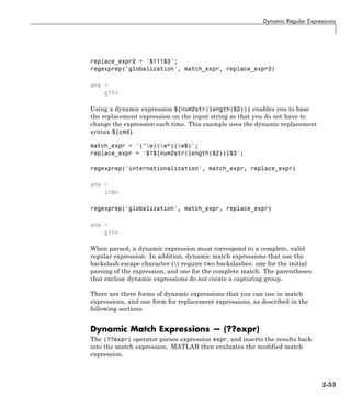
![Dynamic Regular Expressions
m
i
s
ans =
'mississippi'
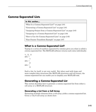
To demonstrate how versatile this type of dynamic expression can be, consider
the next example that progressively assembles a cell array as MATLAB
iteratively parses the input string. The (?!) operator found at the end of the
expression is actually an empty lookahead operator, and forces a failure at
each iteration. This forced failure is necessary if you want to trace the steps
that MATLAB is taking to resolve the expression.
MATLAB makes a number of passes through the input string, each time
trying another combination of letters to see if a fit better than last match can
be found. On any passes in which no matches are found, the test results in
an empty string. The dynamic script (?@if(~isempty($&))) serves to omit
these strings from the matches cell array:
matches = {};
expr = ['(Eulers)?(Cauchys)?(Boole)?(?@if(~isempty($&)),' ...
'matches{end+1}=$&;end)(?!)'];
regexp('Euler Cauchy Boole', expr);
matches
matches =
'Euler Cauchy Boole' 'Euler Cauchy ' 'Euler '
'Cauchy Boole' 'Cauchy ' 'Boole'
The operators $& (or the equivalent $0), $`, and $' refer to that part of the
input string that is currently a match, all characters that precede the current
match, and all characters to follow the current match, respectively. These
operators are sometimes useful when working with dynamic expressions,
particularly those that employ the (?@cmd) operator.
This example parses the input string looking for the letter g. At each iteration
through the string, regexp compares the current character with g, and not
2-57](https://image.slidesharecdn.com/matlabprog-220902050722-ff974cdf/85/matlab_prog-pdf-113-320.jpg)
![2 Program Components
finding it, advances to the next character. The example tracks the progress of
scan through the string by marking the current location being parsed with a
^ character.
(The $` and $· operators capture that part of the string that precedes and
follows the current parsing location. You need two single-quotation marks
($'') to express the sequence $· when it appears within a string.)
str = 'abcdefghij';
expr = '(?@disp(sprintf(''starting match: [%s^%s]'',$`,$'')))g';
regexp(str, expr, 'once');
starting match: [^abcdefghij]
starting match: [a^bcdefghij]
starting match: [ab^cdefghij]
starting match: [abc^defghij]
starting match: [abcd^efghij]
starting match: [abcde^fghij]
starting match: [abcdef^ghij]
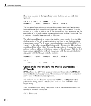
Commands in Replacement Expressions — ${cmd}
The ${cmd} operator modifies the contents of a regular expression replacement
string, making this string adaptable to parameters in the input string that
might vary from one use to the next. As with the other dynamic expressions
used in MATLAB, you can include any number of these expressions within
the overall replacement expression.
In the regexprep call shown here, the replacement string is
'${convertMe($1,$2)}'. In this case, the entire replacement string is a
dynamic expression:
regexprep('This highway is 125 miles long', ...
'(d+.?d*)W(w+)', '${convertMe($1,$2)}');
The dynamic expression tells MATLAB to execute a function named
convertMe using the two tokens (d+.?d*) and (w+), derived from the
string being matched, as input arguments in the call to convertMe. The
replacement string requires a dynamic expression because the values of $1
and $2 are generated at runtime.
2-58](https://image.slidesharecdn.com/matlabprog-220902050722-ff974cdf/85/matlab_prog-pdf-114-320.jpg)
![Dynamic Regular Expressions
The following example defines the file named convertMe that converts
measurements from imperial units to metric.
function valout = convertMe(valin, units)
switch(units)
case 'inches'
fun = @(in)in .* 2.54; uout = 'centimeters';
case 'miles'
fun = @(mi)mi .* 1.6093; uout = 'kilometers';
case 'pounds'
fun = @(lb)lb .* 0.4536; uout = 'kilograms';
case 'pints'
fun = @(pt)pt .* 0.4731; uout = 'litres';
case 'ounces'
fun = @(oz)oz .* 28.35; uout = 'grams';
end
val = fun(str2num(valin));
valout = [num2str(val) ' ' uout];
end
At the command line, call the convertMe function from regexprep, passing in
values for the quantity to be converted and name of the imperial unit:
regexprep('This highway is 125 miles long', ...
'(d+.?d*)W(w+)', '${convertMe($1,$2)}')
ans =
This highway is 201.1625 kilometers long
regexprep('This pitcher holds 2.5 pints of water', ...
'(d+.?d*)W(w+)', '${convertMe($1,$2)}')
ans =
This pitcher holds 1.1828 litres of water
regexprep('This stone weighs about 10 pounds', ...
'(d+.?d*)W(w+)', '${convertMe($1,$2)}')
ans =
This stone weighs about 4.536 kilograms
2-59](https://image.slidesharecdn.com/matlabprog-220902050722-ff974cdf/85/matlab_prog-pdf-115-320.jpg)
![2 Program Components
C = cell(4, 6);
for k = 1:24, C{k} = k * 2; end
C
C =
[2] [10] [18] [26] [34] [42]
[4] [12] [20] [28] [36] [44]
[6] [14] [22] [30] [38] [46]
[8] [16] [24] [32] [40] [48]
extracting the fifth column generates the following comma-separated list:
C{:, 5}
ans =
34
ans =
36
ans =
38
ans =
40
This is the same as explicitly typing
C{1, 5}, C{2, 5}, C{3, 5}, C{4, 5}
Generating a List from a Structure
For structures, extracting a field of the structure that exists across one of its
dimensions yields a comma-separated list.
Start by converting the cell array used above into a 4-by-1 MATLAB structure
with six fields: f1 through f6. Read field f5 for all rows and MATLAB returns
a comma-separated list:
S = cell2struct(C, {'f1', 'f2', 'f3', 'f4', 'f5', 'f6'}, 2);
S.f5
ans =
34
ans =
2-62](https://image.slidesharecdn.com/matlabprog-220902050722-ff974cdf/85/matlab_prog-pdf-118-320.jpg)
![Comma-Separated Lists
36
ans =
38
ans =
40
This is the same as explicitly typing
S(1).f5, S(2).f5, S(3).f5, S(4).f5
Assigning Output from a Comma-Separated List
You can assign any or all consecutive elements of a comma-separated list to
variables with a simple assignment statement. Using the cell array C from
the previous section, assign the first row to variables c1 through c6:
C = cell(4, 6);
for k = 1:24, C{k} = k * 2; end
[c1 c2 c3 c4 c5 c6] = C{1,1:6};
c5
c5 =
34
If you specify fewer output variables than the number of outputs returned by
the expression, MATLAB assigns the first N outputs to those N variables, and
then discards any remaining outputs. In this next example, MATLAB assigns
C{1,1:3} to the variables c1, c2, and c3, and then discards C{1,4:6}:
[c1 c2 c3] = C{1,1:6};
You can assign structure outputs in the same manner:
S = cell2struct(C, {'f1', 'f2', 'f3', 'f4', 'f5', 'f6'}, 2);
[sf1 sf2 sf3] = S.f5;
sf3
sf3 =
38
2-63](https://image.slidesharecdn.com/matlabprog-220902050722-ff974cdf/85/matlab_prog-pdf-119-320.jpg)
![2 Program Components
You also can use the deal function for this purpose.
Assigning to a Comma-Separated List
The simplest way to assign multiple values to a comma-separated list is to
use the deal function. This function distributes all of its input arguments to
the elements of a comma-separated list.
This example initializes a comma-separated list to a set of vectors in a cell
array, and then uses deal to overwrite each element in the list:
c{1} = [31 07]; c{2} = [03 78];
c{:}
ans =
31 7
ans =
3 78
[c{:}] = deal([10 20],[14 12]);
c{:}
ans =
10 20
ans =
14 12
This example does the same as the one above, but with a comma-separated
list of vectors in a structure field:
s(1).field1 = [31 07]; s(2).field1 = [03 78];
s.field1
ans =
31 7
ans =
3 78
2-64](https://image.slidesharecdn.com/matlabprog-220902050722-ff974cdf/85/matlab_prog-pdf-120-320.jpg)
![Comma-Separated Lists
[s.field1] = deal([10 20],[14 12]);
s.field1
ans =
10 20
ans =
14 12
How to Use the Comma-Separated Lists
Common uses for comma-separated lists are
• “Constructing Arrays” on page 2-65
• “Displaying Arrays” on page 2-66
• “Concatenation” on page 2-66
• “Function Call Arguments” on page 2-66
• “Function Return Values” on page 2-67
The following sections provide examples of using comma-separated lists with
cell arrays. Each of these examples applies to MATLAB structures as well.
Constructing Arrays
You can use a comma-separated list to enter a series of elements when
constructing a matrix or array. Note what happens when you insert a list of
elements as opposed to adding the cell itself.
When you specify a list of elements with C{:, 5}, MATLAB inserts the four
individual elements:
A = {'Hello', C{:, 5}, magic(4)}
A =
'Hello' [34] [36] [38] [40] [4x4 double]
When you specify the C cell itself, MATLAB inserts the entire cell array:
A = {'Hello', C, magic(4)}
A =
'Hello' {4x6 cell} [4x4 double]
2-65](https://image.slidesharecdn.com/matlabprog-220902050722-ff974cdf/85/matlab_prog-pdf-121-320.jpg)
![2 Program Components
Displaying Arrays
Use a list to display all or part of a structure or cell array:
A{:}
ans =
Hello
ans =
34
ans =
36
ans =
38
.
.
.
Concatenation
Putting a comma-separated list inside square brackets extracts the specified
elements from the list and concatenates them:
A = [C{:, 5:6}]
A =
34 36 38 40 42 44 46 48
whos A
Name Size Bytes Class
A 1x8 64 double array
Function Call Arguments
When writing the code for a function call, you enter the input arguments as a
list with each argument separated by a comma. If you have these arguments
stored in a structure or cell array, then you can generate all or part of the
argument list from the structure or cell array instead. This can be especially
useful when passing in variable numbers of arguments.
2-66](https://image.slidesharecdn.com/matlabprog-220902050722-ff974cdf/85/matlab_prog-pdf-122-320.jpg)
![Comma-Separated Lists
This example passes several attribute-value arguments to the plot function:
X = -pi:pi/10:pi;
Y = tan(sin(X)) - sin(tan(X));
C{1,1} = 'LineWidth'; C{2,1} = 2;
C{1,2} = 'MarkerEdgeColor'; C{2,2} = 'k';
C{1,3} = 'MarkerFaceColor'; C{2,3} = 'g';
plot(X, Y, '--rs', C{:})
Function Return Values
MATLAB functions can also return more than one value to the caller. These
values are returned in a list with each value separated by a comma. Instead
of listing each return value, you can use a comma-separated list with a
structure or cell array. This becomes more useful for those functions that
have variable numbers of return values.
This example returns three values to a cell array:
C = cell(1, 3);
[C{:}] = fileparts('work/mytests/strArrays.mat')
C =
'work/mytests' 'strArrays' '.mat'
Fast Fourier Transform Example
The fftshift function swaps the left and right halves of each dimension of
an array. For a simple vector such as [0 2 4 6 8 10] the output would be
[6 8 10 0 2 4]. For a multidimensional array, fftshift performs this
swap along each dimension.
fftshift uses vectors of indices to perform the swap. For the vector shown
above, the index [1 2 3 4 5 6] is rearranged to form a new index [4 5 6 1
2 3]. The function then uses this index vector to reposition the elements. For
a multidimensional array, fftshift must construct an index vector for each
dimension. A comma-separated list makes this task much simpler.
Here is the fftshift function:
function y = fftshift(x)
2-67](https://image.slidesharecdn.com/matlabprog-220902050722-ff974cdf/85/matlab_prog-pdf-123-320.jpg)
![2 Program Components
numDims = ndims(x);
idx = cell(1, numDims);
for k = 1:numDims
m = size(x, k);
p = ceil(m/2);
idx{k} = [p+1:m 1:p];
end
y = x(idx{:});
The function stores the index vectors in cell array idx. Building this cell array
is relatively simple. For each of the N dimensions, determine the size of that
dimension and find the integer index nearest the midpoint. Then, construct a
vector that swaps the two halves of that dimension.
By using a cell array to store the index vectors and a comma-separated list
for the indexing operation, fftshift shifts arrays of any dimension using
just a single operation: y = x(idx{:}). If you were to use explicit indexing,
you would need to write one if statement for each dimension you want the
function to handle:
if ndims(x) == 1
y = x(index1);
else if ndims(x) == 2
y = x(index1, index2);
end
Another way to handle this without a comma-separated list would be to loop
over each dimension, converting one dimension at a time and moving data
each time. With a comma-separated list, you move the data just once. A
comma-separated list makes it very easy to generalize the swapping operation
to an arbitrary number of dimensions.
2-68](https://image.slidesharecdn.com/matlabprog-220902050722-ff974cdf/85/matlab_prog-pdf-124-320.jpg)
![2 Program Components
For example, create a cell array that contains 10 elements, where each
element is a numeric array:
numArrays = 10;
A = cell(numArrays,1);
for n = 1:numArrays
A{n} = magic(n);
end
Access the data in the cell array by indexing with curly braces. For example,
display the fifth element of A:
A{5}
ans =
17 24 1 8 15
23 5 7 14 16
4 6 13 20 22
10 12 19 21 3
11 18 25 2 9
The assignment statement A{n} = magic(n) is more elegant and efficient
than this call to eval:
eval(['A', int2str(n),' = magic(n)']) % Not recommended
For more information, see:
• “Create a Cell Array” on page 10-3
• “Create a Structure Array” on page 9-2
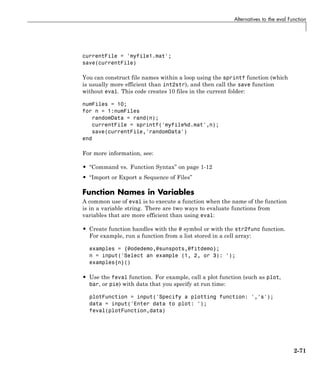
Files with Sequential Names
Related data files often have a common root name with an integer index, such
as myfile1.mat through myfileN.mat. A common (but not recommended) use
of the eval function is to construct and pass each file name to a function
using command syntax, such as
eval(['save myfile',int2str(n),'.mat']) % Not recommended
The best practice is to use function syntax, which allows you to pass variables
as inputs. For example:
2-70](https://image.slidesharecdn.com/matlabprog-220902050722-ff974cdf/85/matlab_prog-pdf-126-320.jpg)
![2 Program Components
Field Names in Variables
Access data in a structure with a variable field name by enclosing the
expression for the field in parentheses. For example:
myData.height = [67, 72, 58];
myData.weight = [140, 205, 90];
fieldName = input('Select data (height or weight): ','s');
dataToUse = myData.(fieldName);
If you enter weight at the input prompt, then you can find the minimum
weight value with the following command.
min(dataToUse)
ans =
90
For an additional example, see “Generate Field Names from Variables” on
page 9-11.
Error Handling
The preferred method for error handling in MATLAB is to use a try, catch
statement. For example:
try
B = A;
catch exception
disp('A is undefined')
end
If your workspace does not contain variable A, then this code returns:
A is undefined
Previous versions of the documentation for the eval function include the
syntax eval(expression,catch_expr). If evaluating the expression input
returns an error, then eval evaluates catch_expr. However, an explicit
try/catch is significantly clearer than an implicit catch in an eval statement.
Using the implicit catch is not recommended.
2-72](https://image.slidesharecdn.com/matlabprog-220902050722-ff974cdf/85/matlab_prog-pdf-128-320.jpg)
![2 Program Components
Symbol Reference
In this section...
“Asterisk — *” on page 2-74
“At — @” on page 2-75
“Colon — :” on page 2-76
“Comma — ,” on page 2-77
“Curly Braces — { }” on page 2-78
“Dot — .” on page 2-78
“Dot-Dot — ..” on page 2-79
“Dot-Dot-Dot (Ellipsis) — ...” on page 2-79
“Dot-Parentheses — .( )” on page 2-80
“Exclamation Point — !” on page 2-81
“Parentheses — ( )” on page 2-81
“Percent — %” on page 2-82
“Percent-Brace — %{ %}” on page 2-82
“Plus — +” on page 2-83
“Semicolon — ;” on page 2-83
“Single Quotes — ’ ’” on page 2-84
“Space Character” on page 2-84
“Slash and Backslash — / ” on page 2-85
“Square Brackets — [ ]” on page 2-85
“Tilde — ~” on page 2-86
Asterisk — *
An asterisk in a filename specification is used as a wildcard specifier, as
described below.
2-74](https://image.slidesharecdn.com/matlabprog-220902050722-ff974cdf/85/matlab_prog-pdf-130-320.jpg)
![Symbol Reference
B = A(7, 1:5); % Read columns 1-5 of row 7.
B = A(4:2:8, 1:5); % Read columns 1-5 of rows 4, 6, and 8.
B = A(:, 1:5); % Read columns 1-5 of all rows.
Conversion to Column Vector
Convert a matrix or array to a column vector using the colon operator as a
single index:
A = rand(3,4);
B = A(:);
Preserving Array Shape on Assignment
Using the colon operator on the left side of an assignment statement, you can
assign new values to array elements without changing the shape of the array:
A = rand(3,4);
A(:) = 1:12;
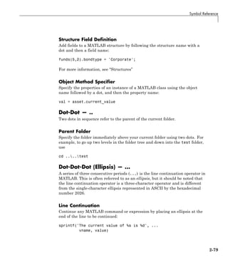
Comma — ,
A comma is used to separate the following types of elements.
Row Element Separator
When constructing an array, use a comma to separate elements that belong
in the same row:
A = [5.92, 8.13, 3.53]
Array Index Separator
When indexing into an array, use a comma to separate the indices into each
dimension:
X = A(2, 7, 4)
2-77](https://image.slidesharecdn.com/matlabprog-220902050722-ff974cdf/85/matlab_prog-pdf-133-320.jpg)
![2 Program Components
Function Input and Output Separator
When calling a function, use a comma to separate output and input
arguments:
function [data, text] = xlsread(file, sheet, range, mode)
Command or Statement Separator
To enter more than one MATLAB command or statement on the same line,
separate each command or statement with a comma:
for k = 1:10, sum(A(k)), end
Curly Braces — { }
Use curly braces to construct or get the contents of cell arrays.
Cell Array Constructor
To construct a cell array, enclose all elements of the array in curly braces:
C = {[2.6 4.7 3.9], rand(8)*6, 'C. Coolidge'}
Cell Array Indexing
Index to a specific cell array element by enclosing all indices in curly braces:
A = C{4,7,2}
For more information, see “Cell Arrays”
Dot — .
The single dot operator has the following different uses in MATLAB.
Decimal Point
MATLAB uses a period to separate the integral and fractional parts of a
number.
2-78](https://image.slidesharecdn.com/matlabprog-220902050722-ff974cdf/85/matlab_prog-pdf-134-320.jpg)
![2 Program Components
Entering Long Strings. You cannot use an ellipsis within single quotes
to continue a string to the next line:
string = 'This is not allowed and will generate an ...
error in MATLAB.'
To enter a string that extends beyond a single line, piece together shorter
strings using either the concatenation operator ([]) or the sprintf function.
Here are two examples:
quote1 = [
'Tiger, tiger, burning bright in the forests of the night,' ...
'what immortal hand or eye could frame thy fearful symmetry?'];
quote2 = sprintf('%s%s%s', ...
'In Xanadu did Kubla Khan a stately pleasure-dome decree,', ...
'where Alph, the sacred river, ran ', ...
'through caverns measureless to man down to a sunless sea.');
Defining Arrays. MATLAB interprets the ellipsis as a space character. For
statements that define arrays or cell arrays within [] or {} operators, a space
character separates array elements. For example,
not_valid = [1 2 zeros...
(1,3)]
is equivalent to
not_valid = [1 2 zeros (1,3)]
which returns an error. Place the ellipses so that the interpreted statement
is valid, such as
valid = [1 2 ...
zeros(1,3)]
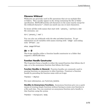
Dot-Parentheses — .( )
Use dot-parentheses to specify the name of a dynamic structure field.
2-80](https://image.slidesharecdn.com/matlabprog-220902050722-ff974cdf/85/matlab_prog-pdf-136-320.jpg)
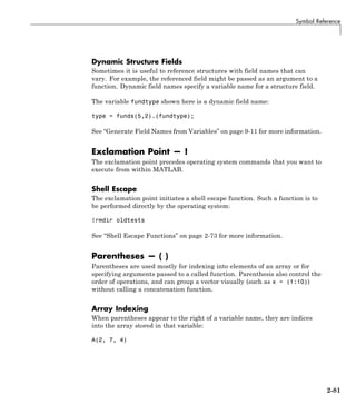
![Symbol Reference
%{
The purpose of this routine is to compute
the value of ...
%}
Note With the exception of whitespace characters, the %{ and %} operators
must appear alone on the lines that immediately precede and follow the block
of help text. Do not include any other text on these lines.
Plus — +
The + sign appears most frequently as an arithmetic operator, but is also
used to designate the names of package folders. For more information, see
“Packages Create Namespaces”.
Semicolon — ;
The semicolon can be used to construct arrays, suppress output from a
MATLAB command, or to separate commands entered on the same line.
Array Row Separator
When used within square brackets to create a new array or concatenate
existing arrays, the semicolon creates a new row in the array:
A = [5, 8; 3, 4]
A =
5 8
3 4
Output Suppression
When placed at the end of a command, the semicolon tells MATLAB not to
display any output from that command. In this example, MATLAB does not
display the resulting 100-by-100 matrix:
A = ones(100, 100);
2-83](https://image.slidesharecdn.com/matlabprog-220902050722-ff974cdf/85/matlab_prog-pdf-139-320.jpg)
![2 Program Components
Command or Statement Separator
Like the comma operator, you can enter more than one MATLAB command
on a line by separating each command with a semicolon. MATLAB suppresses
output for those commands terminated with a semicolon, and displays the
output for commands terminated with a comma.
In this example, assignments to variables A and C are terminated with
a semicolon, and thus do not display. Because the assignment to B is
comma-terminated, the output of this one command is displayed:
A = 12.5; B = 42.7, C = 1.25;
B =
42.7000
Single Quotes — ’ ’
Single quotes are the constructor symbol for MATLAB character arrays.
Character and String Constructor
MATLAB constructs a character array from all characters enclosed in single
quotes. If only one character is in quotes, then MATLAB constructs a 1-by-1
array:
S = 'Hello World'
For more information, see “Characters and Strings”
Space Character
The space character serves a purpose similar to the comma in that it can be
used to separate row elements in an array constructor, or the values returned
by a function.
Row Element Separator
You have the option of using either commas or spaces to delimit the row
elements of an array when constructing the array. To create a 1-by-3 array,
use
A = [5.92 8.13 3.53]
2-84](https://image.slidesharecdn.com/matlabprog-220902050722-ff974cdf/85/matlab_prog-pdf-140-320.jpg)
![Symbol Reference
A =
5.9200 8.1300 3.5300
When indexing into an array, you must always use commas to reference each
dimension of the array.
Function Output Separator
Spaces are allowed when specifying a list of values to be returned by a
function. You can use spaces to separate return values in both function
declarations and function calls:
function [data text] = xlsread(file, sheet, range, mode)
Slash and Backslash — /
The slash (/) and backslash () characters separate the elements of a path or
folder string. On Microsoft Windows-based systems, both slash and backslash
have the same effect. On The Open Group UNIX-based systems, you must
use slash only.
On a Windows system, you can use either backslash or slash:
dir([matlabroot 'toolboxmatlabelmatshiftdim.m'])
dir([matlabroot '/toolbox/matlab/elmat/shiftdim.m'])
On a UNIX system, use only the forward slash:
dir([matlabroot '/toolbox/matlab/elmat/shiftdim.m'])
Square Brackets — [ ]
Square brackets are used in array construction and concatenation, and also in
declaring and capturing values returned by a function.
Array Constructor
To construct a matrix or array, enclose all elements of the array in square
brackets:
A = [5.7, 9.8, 7.3; 9.2, 4.5, 6.4]
2-85](https://image.slidesharecdn.com/matlabprog-220902050722-ff974cdf/85/matlab_prog-pdf-141-320.jpg)
![2 Program Components
Concatenation
To combine two or more arrays into a new array through concatenation,
enclose all array elements in square brackets:
A = [B, eye(6), diag([0:2:10])]
Function Declarations and Calls
When declaring or calling a function that returns more than one output,
enclose each return value that you need in square brackets:
[data, text] = xlsread(file, sheet, range, mode)
Tilde — ~
The tilde character is used in comparing arrays for unequal values, finding
the logical NOT of an array, and as a placeholder for an input or output
argument you want to omit from a function call.
Not Equal to
To test for inequality values of elements in arrays a and b for inequality,
use a~=b:
a = primes(29); b = [2 4 6 7 11 13 20 22 23 29];
not_prime = b(a~=b)
not_prime =
4 6 20 22
Logical NOT
To find those elements of an array that are zero, use:
a = [35 42 0 18 0 0 0 16 34 0];
~a
ans =
0 0 1 0 1 1 1 0 0 1
2-86](https://image.slidesharecdn.com/matlabprog-220902050722-ff974cdf/85/matlab_prog-pdf-142-320.jpg)
![Symbol Reference
Argument Placeholder
To have the fileparts function return its third output value and skip the
first two, replace arguments one and two with a tilde character:
[~, ~, filenameExt] = fileparts(fileSpec);
See “Ignore Function Inputs” on page 18-13 in the MATLAB Programming
documentation for more information.
2-87](https://image.slidesharecdn.com/matlabprog-220902050722-ff974cdf/85/matlab_prog-pdf-143-320.jpg)


![Integers
according to the default rounding algorithm. The example below yields an
exact answer of 1426.75 which MATLAB then rounds to the next highest
integer:
int16(325) * 4.39
ans =
1427
The integer conversion functions are also useful when converting other
classes, such as strings, to integers:
str = 'Hello World';
int8(str)
ans =
72 101 108 108 111 32 87 111 114 108 100
Arithmetic Operations on Integer Classes
MATLAB can perform integer arithmetic on the following types of data:
• Integers or integer arrays of the same integer data type. This yields a
result that has the same data type as the operands:
x = uint32([132 347 528]) .* uint32(75);
class(x)
ans =
uint32
• Integers or integer arrays and scalar double-precision floating-point
numbers. This yields a result that has the same data type as the integer
operands:
x = uint32([132 347 528]) .* 75.49;
class(x)
ans =
uint32
For all binary operations in which one operand is an array of integer data
type (except 64-bit integers) and the other is a scalar double, MATLAB
computes the operation using elementwise double-precision arithmetic, and
then converts the result back to the original integer data type. For binary
4-5](https://image.slidesharecdn.com/matlabprog-220902050722-ff974cdf/85/matlab_prog-pdf-157-320.jpg)
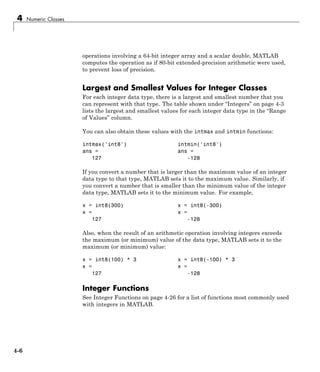
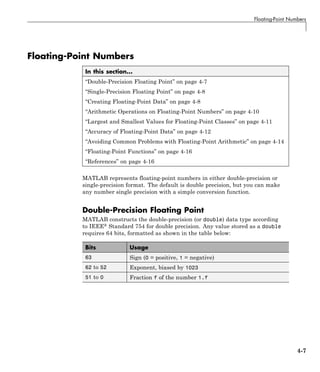
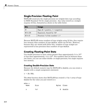
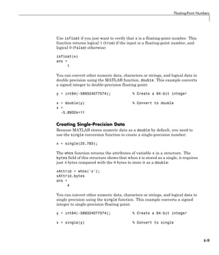
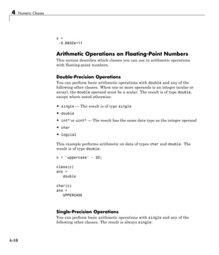
![Floating-Point Numbers
• single
• double
• char
• logical
In this example, 7.5 defaults to type double, and the result is of type single:
x = single([1.32 3.47 5.28]) .* 7.5;
class(x)
ans =
single
Largest and Smallest Values for Floating-Point
Classes
For the double and single classes, there is a largest and smallest number
that you can represent with that type.
Largest and Smallest Double-Precision Values
The MATLAB functions realmax and realmin return the maximum and
minimum values that you can represent with the double data type:
str = 'The range for double is:nt%g to %g andnt %g to %g';
sprintf(str, -realmax, -realmin, realmin, realmax)
ans =
The range for double is:
-1.79769e+308 to -2.22507e-308 and
2.22507e-308 to 1.79769e+308
Numbers larger than realmax or smaller than -realmax are assigned the
values of positive and negative infinity, respectively:
realmax + .0001e+308
ans =
Inf
-realmax - .0001e+308
4-11](https://image.slidesharecdn.com/matlabprog-220902050722-ff974cdf/85/matlab_prog-pdf-163-320.jpg)
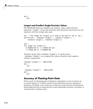
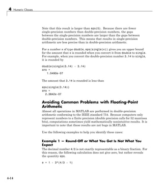
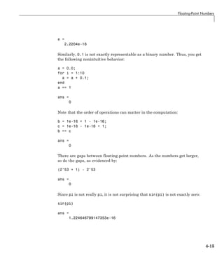
![4 Numeric Classes
Example 2 — Catastrophic Cancellation
When subtractions are performed with nearly equal operands, sometimes
cancellation can occur unexpectedly. The following is an example of a
cancellation caused by swamping (loss of precision that makes the addition
insignificant).
sqrt(1e-16 + 1) - 1
ans =
0
Some functions in MATLAB, such as expm1 and log1p, may be used to
compensate for the effects of catastrophic cancellation.
Example 3 — Floating-Point Operations and Linear Algebra
Round-off, cancellation, and other traits of floating-point arithmetic combine
to produce startling computations when solving the problems of linear
algebra. MATLAB warns that the following matrix A is ill-conditioned, and
therefore the system Ax = b may be sensitive to small perturbations:
A = diag([2 eps]);
b = [2; eps];
y = Ab;
Warning: Matrix is close to singular or badly scaled.
Results may be inaccurate. RCOND = 1.110223e-16.
These are only a few of the examples showing how IEEE floating-point
arithmetic affects computations in MATLAB. Note that all computations
performed in IEEE 754 arithmetic are affected, this includes applications
written in C or FORTRAN, as well as MATLAB.
Floating-Point Functions
See Floating-Point Functions on page 4-27 for a list of functions most
commonly used with floating-point numbers in MATLAB.
References
The following references provide more information about floating-point
arithmetic.
4-16](https://image.slidesharecdn.com/matlabprog-220902050722-ff974cdf/85/matlab_prog-pdf-168-320.jpg)
![Floating-Point Numbers
References
[1] Moler, Cleve, “Floating Points,” MATLAB News and Notes, Fall,
1996. A PDF version is available on the MathWorks Web site at
http://www.mathworks.com/company/newsletters/news_notes/pdf/Fall96Cleve.pdf
[2] Moler, Cleve, Numerical Computing with MATLAB, S.I.A.M.
A PDF version is available on the MathWorks Web site at
http://www.mathworks.com/moler/.
4-17](https://image.slidesharecdn.com/matlabprog-220902050722-ff974cdf/85/matlab_prog-pdf-169-320.jpg)
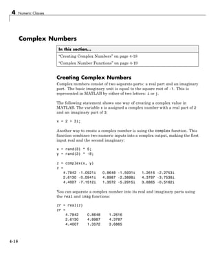
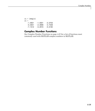
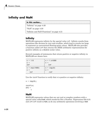
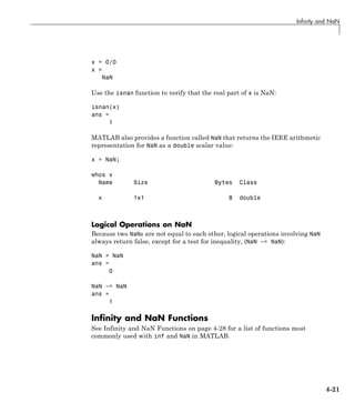
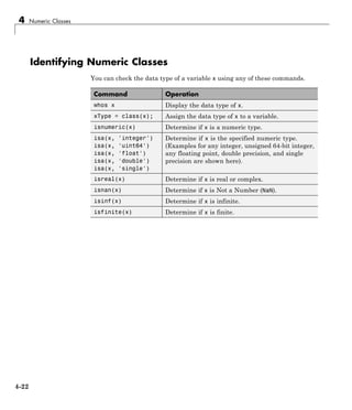
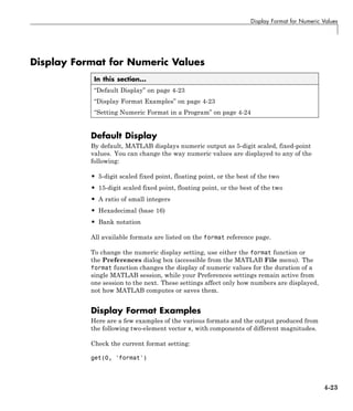
![4 Numeric Classes
ans =
short
Set the value for x and display in 5-digit scaled fixed point:
x = [4/3 1.2345e-6]
x =
1.3333 0.0000
Set the format to 5-digit floating point:
format short e
x
x =
1.3333e+00 1.2345e-06
Set the format to 15-digit scaled fixed point:
format long
x
x =
1.333333333333333 0.000001234500000
Set the format to 'rational' for small integer ratio output:
format rational
x
x =
4/3 1/810045
Set an integer value for x and display it in hexadecimal (base 16) format:
format hex
x = uint32(876543210)
x =
343efcea
Setting Numeric Format in a Program
To temporarily change the numeric format inside a program, get the original
format using the get function and save it in a variable. When you finish
4-24](https://image.slidesharecdn.com/matlabprog-220902050722-ff974cdf/85/matlab_prog-pdf-176-320.jpg)
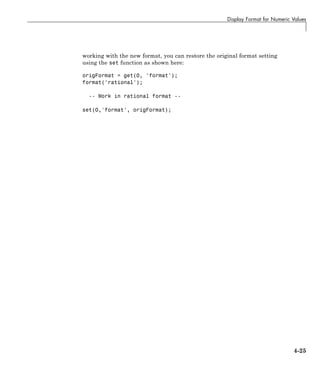
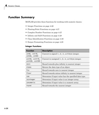
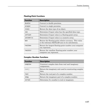
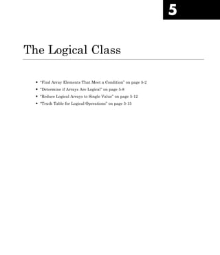
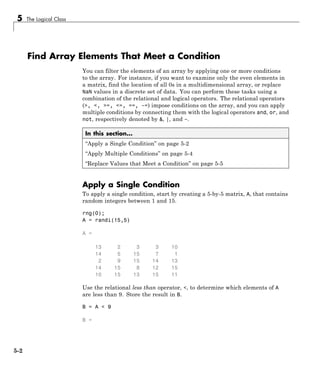
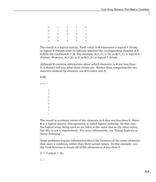
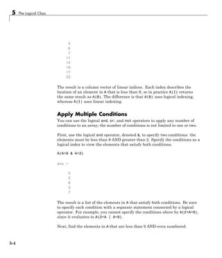
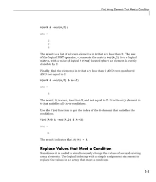
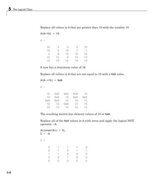
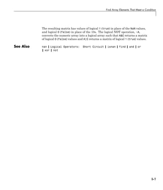
![5 The Logical Class
Determine if Arrays Are Logical
To determine whether an array is logical, you can test the entire array or each
element individually. This is useful when you want to confirm the output
data type of a function.
This page shows several ways to determine if an array is logical.
In this section...
“Identify Logical Matrix” on page 5-8
“Test an Entire Array” on page 5-9
“Test Each Array Element” on page 5-9
“Summary Table” on page 5-10
Identify Logical Matrix
Create a 3-by-6 matrix and locate all elements greater than 0.5.
A = gallery('uniformdata',[3,6],0) > 0.5
A =
1 0 0 0 1 0
0 1 0 1 1 1
1 1 1 1 0 1
The result, A, is a 3-by-6 logical matrix.
Use the whos function to confirm the size, byte count, and class (or data type)
of the matrix, A.
whos A
Name Size Bytes Class Attributes
A 3x6 18 logical
The result confirms that A is a 3-by-6 logical matrix.
5-8](https://image.slidesharecdn.com/matlabprog-220902050722-ff974cdf/85/matlab_prog-pdf-188-320.jpg)
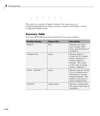
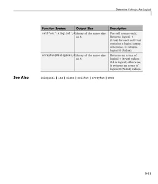
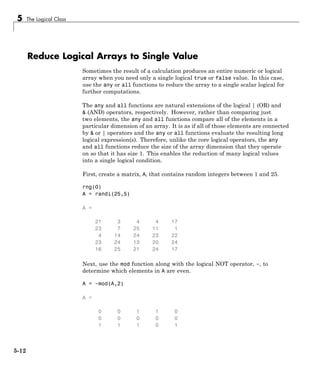
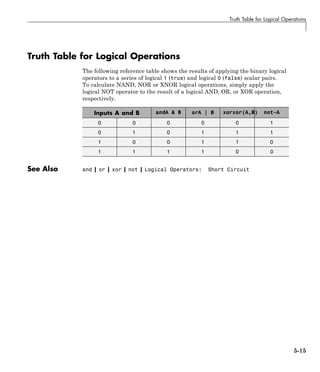

![Creating Character Arrays
str_alpha = char([72 101 108 108 111])
str_alpha =
Hello
Creating a Rectangular Character Array
You can join two or more strings together to create a new character array.
This is called concatenation and is explained for numeric arrays in the
section “Concatenating Matrices”. As with numeric arrays, you can combine
character arrays vertically or horizontally to create a new character array.
Alternatively, combine strings into a cell array. Cell arrays are flexible
containers that allow you to easily combine strings of varying length.
Combining Strings Vertically
To combine strings into a two-dimensional character array, use either of these
methods:
• Apply the MATLAB concatenation operator, []. Separate each row with a
semicolon (;). Each row must contain the same number of characters. For
example, combine three strings of equal length:
dev_title = ['Thomas R. Lee'; ...
'Sr. Developer'; ...
'SFTware Corp.'];
If the strings have different lengths, pad with space characters as needed.
For example:
mgr_title = ['Harold A. Jorgensen '; ...
'Assistant Project Manager'; ...
'SFTware Corp. '];
• Call the char function. If the strings are different length, char pads the
shorter strings with trailing blanks so that each row has the same number
of characters. For example, combine three strings of different lengths:
mgr_title = char('Harold A. Jorgensen', ...
'Assistant Project Manager', 'SFTware Corp.');
6-3](https://image.slidesharecdn.com/matlabprog-220902050722-ff974cdf/85/matlab_prog-pdf-199-320.jpg)
![6 Characters and Strings
The char function creates a 3-by-25 character array mgr_title.
Combining Strings Horizontally
To combine strings into a single row vector, use either of these methods:
• Apply the MATLAB concatenation operator, []. Separate the input strings
with a comma or a space. This method preserves any trailing spaces in the
input arrays. For example, combine several strings:
name = 'Thomas R. Lee';
title = 'Sr. Developer';
company = 'SFTware Corp.';
full_name = [name ', ' title ', ' company]
MATLAB returns
full_name =
Thomas R. Lee, Sr. Developer, SFTware Corp.
• Call the string concatenation function, strcat. This method removes
trailing spaces in the inputs. For example, combine strings to create a
hypothetical email address:
name = 'myname ';
domain = 'mydomain ';
ext = 'com ';
address = strcat(name, '@', domain, '.', ext)
MATLAB returns
address =
myname@mydomain.com
Identifying Characters in a String
Use any of the following functions to identify a character or string, or certain
characters in a string:
6-4](https://image.slidesharecdn.com/matlabprog-220902050722-ff974cdf/85/matlab_prog-pdf-200-320.jpg)
![Creating Character Arrays
Function Description
ischar Determine whether the input is a character array.
isletter Find all alphabetic letters in the input string.
isspace Find all space characters in the input string.
isstrprop Find all characters of a specific category.
str = 'Find the space characters in this string';
% | | | | | |
% 5 9 15 26 29 34
find(isspace(str))
ans =
5 9 15 26 29 34
Working with Space Characters
The blanks function creates a string of space characters. The following
example creates a string of 15 space characters:
s = blanks(15)
s =
To make the example more useful, append a '|' character to the beginning
and end of the blank string so that you can see the output:
['|' s '|'] % Make result visible.
ans =
| |
Insert a few nonspace characters in the middle of the blank string:
s(6:10) = 'AAAAA';
['|' s '|'] % Make result visible.
ans =
| AAAAA |
You can justify the positioning of these characters to the left or right using
the strjust function:
6-5](https://image.slidesharecdn.com/matlabprog-220902050722-ff974cdf/85/matlab_prog-pdf-201-320.jpg)
![6 Characters and Strings
sLeft = strjust(s, 'left');
['|' sLeft '|'] % Make result visible.
ans =
|AAAAA |
sRight = strjust(s, 'right');
['|' sRight '|'] % Make result visible.
ans =
| AAAAA|
Remove all trailing space characters with deblank:
sDeblank = deblank(s);
['|' sDeblank '|'] % Make result visible.
ans =
| AAAAA|
Remove all leading and trailing spaces with strtrim:
sTrim = strtrim(s);
['|' sTrim '|'] % Make result visible.
ans =
|AAAAA|
Expanding Character Arrays
Generally, MathWorks does not recommend expanding the size of an existing
character array by assigning additional characters to indices beyond the
bounds of the array such that part of the array becomes padded with zeros.
6-6](https://image.slidesharecdn.com/matlabprog-220902050722-ff974cdf/85/matlab_prog-pdf-202-320.jpg)
![Cell Arrays of Strings
Cell Arrays of Strings
In this section...
“Converting to a Cell Array of Strings” on page 6-7
“Functions for Cell Arrays of Strings” on page 6-8
Converting to a Cell Array of Strings
Creating strings in a regular MATLAB array requires that all strings in the
array be of the same length. This often means that you have to pad blanks at
the end of strings to equalize their length. However, another type of MATLAB
array, the cell array, can hold different sizes and types of data in an array
without padding. Cell arrays provide a more flexible way to store strings of
varying length.
The cellstr function converts a character array into a cell array of strings.
Consider this character array:
data = ['Allison Jones';'Development ';'Phoenix '];
Each row of the matrix is padded so that all have equal length (in this case,
13 characters).
Now use cellstr to create a column vector of cells, each cell containing one
of the strings from the data array:
celldata = cellstr(data)
celldata =
'Allison Jones'
'Development'
'Phoenix'
Note that the cellstr function strips off the blanks that pad the rows of the
input string matrix:
length(celldata{3})
ans =
7
6-7](https://image.slidesharecdn.com/matlabprog-220902050722-ff974cdf/85/matlab_prog-pdf-203-320.jpg)
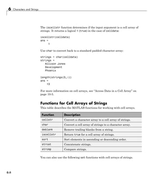
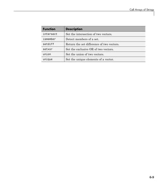
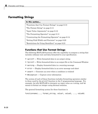
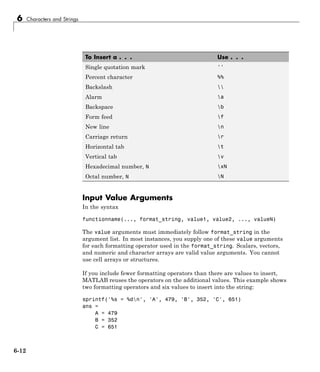
![Formatting Strings
You can also specify multiple value arguments as a vector or matrix. The
format_string needs one %s operator for the entire matrix or vector:
mvec = [77 65 84 76 65 66];
sprintf('%s ', char(mvec))
ans =
MATLAB
Sequential and Numbered Argument Specification
You can place value arguments in the argument list either sequentially (that
is, in the same order in which their formatting operators appear in the string),
or by identifier (adding a number to each operator that identifies which value
argument to replace it with). By default, MATLAB uses sequential ordering.
To specify arguments by a numeric identifier, add a positive integer followed
by a $ sign immediately after the % sign in the operator. Numbered argument
specification is explained in more detail under the topic “Value Identifiers”
on page 6-20.
Ordered Sequentially Ordered By Identifier
sprintf('%s %s %s', ...
'1st', '2nd', '3rd')
ans =
1st 2nd 3rd
sprintf('%3$s %2$s %1$s', ...
'1st', '2nd', '3rd')
ans =
3rd 2nd 1st
The Formatting Operator
Formatting operators tell MATLAB how to format the numeric or character
value arguments and where to insert them into the string. These operators
control the notation, alignment, significant digits, field width, and other
aspects of the output string.
A formatting operator begins with a % character, which may be followed by a
series of one or more numbers, characters, or symbols, each playing a role in
further defining the format of the insertion value. The final entry in this series
is a single conversion character that MATLAB uses to define the notation
6-13](https://image.slidesharecdn.com/matlabprog-220902050722-ff974cdf/85/matlab_prog-pdf-209-320.jpg)
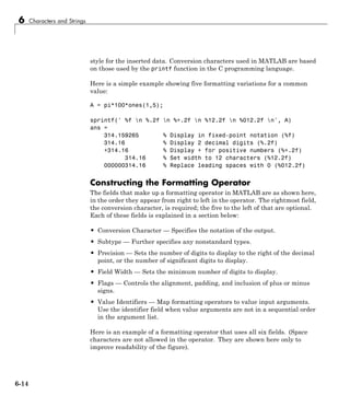
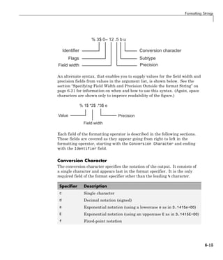
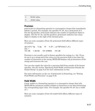
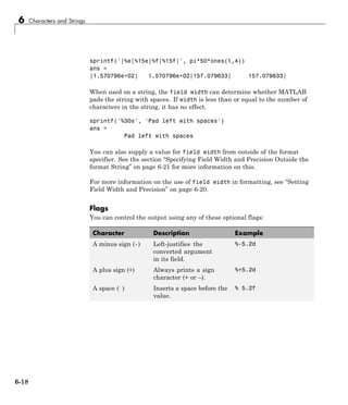
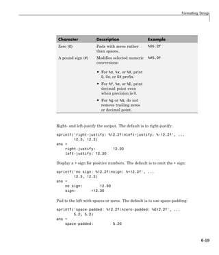
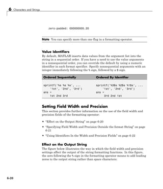
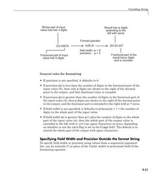
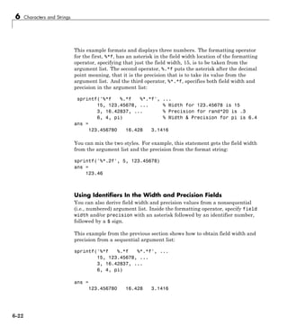
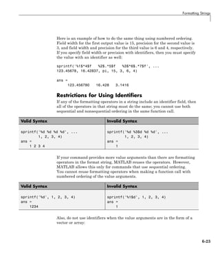
![6 Characters and Strings
Valid Syntax Invalid Syntax
v = [1.4 2.7 3.1];
sprintf('%.4f %.4f %.4f', v)
ans =
1.4000 2.7000 3.1000
v = [1.4 2.7 3.1];
sprintf('%3$.4f %1$.4f %2$.4f', v)
ans =
Empty string: 1-by-0
6-24](https://image.slidesharecdn.com/matlabprog-220902050722-ff974cdf/85/matlab_prog-pdf-220-320.jpg)
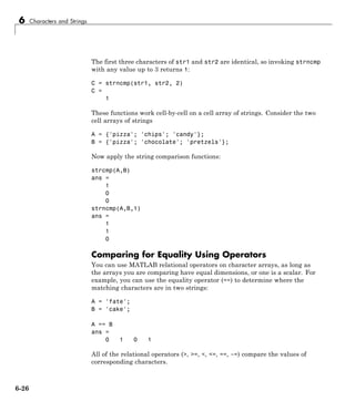
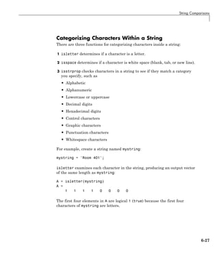
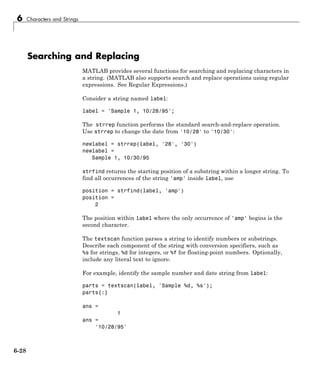
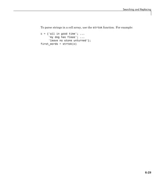
![6 Characters and Strings
Converting from Numeric to String
In this section...
“Function Summary” on page 6-30
“Converting to a Character Equivalent” on page 6-31
“Converting to a String of Numbers” on page 6-31
“Converting to a Specific Radix” on page 6-31
Function Summary
The functions listed in this table provide a number of ways to convert numeric
data to character strings.
Function Description Example
char Convert a positive integer to an equivalent
character. (Truncates any fractional parts.)
[72 105] → 'Hi'
int2str Convert a positive or negative integer to a
character type. (Rounds any fractional parts.)
[72 105] → '72 105'
num2str Convert a numeric type to a character type of the
specified precision and format.
[72 105] →
'72/105/' (format
set to %1d/)
mat2str Convert a numeric type to a character type of the
specified precision, returning a string MATLAB
can evaluate.
[72 105] → '[72
105]'
dec2hex Convert a positive integer to a character type of
hexadecimal base.
[72 105] → '48 69'
dec2bin Convert a positive integer to a character type of
binary base.
[72 105] → '1001000
1101001'
dec2base Convert a positive integer to a character type of
any base from 2 through 36.
[72 105] → '110
151' (base set to 8)
6-30](https://image.slidesharecdn.com/matlabprog-220902050722-ff974cdf/85/matlab_prog-pdf-226-320.jpg)
![Converting from Numeric to String
Converting to a Character Equivalent
The char function converts integers to Unicode character codes and returns a
string composed of the equivalent characters:
x = [77 65 84 76 65 66];
char(x)
ans =
MATLAB
Converting to a String of Numbers
The int2str, num2str, and mat2str functions convert numeric values to
strings where each character represents a separate digit of the input value.
The int2str and num2str functions are often useful for labeling plots. For
example, the following lines use num2str to prepare automated labels for the
x-axis of a plot:
function plotlabel(x, y)
plot(x, y)
str1 = num2str(min(x));
str2 = num2str(max(x));
out = ['Value of f from ' str1 ' to ' str2];
xlabel(out);
Converting to a Specific Radix
Another class of conversion functions changes numeric values into strings
representing a decimal value in another base, such as binary or hexadecimal
representation. This includes dec2hex, dec2bin, and dec2base.
6-31](https://image.slidesharecdn.com/matlabprog-220902050722-ff974cdf/85/matlab_prog-pdf-227-320.jpg)
![6 Characters and Strings
Converting from String to Numeric
In this section...
“Function Summary” on page 6-32
“Converting from a Character Equivalent” on page 6-33
“Converting from a Numeric String” on page 6-33
“Converting from a Specific Radix” on page 6-34
Function Summary
The functions listed in this table provide a number of ways to convert
character strings to numeric data.
Function Description Example
uintN (e.g., uint8) Convert a character to an integer code that
represents that character.
'Hi' → 72 105
str2num Convert a character type to a numeric type. '72 105' → [72 105]
str2double Similar to str2num, but offers better
performance and works with cell arrays of
strings.
{'72' '105'} → [72
105]
hex2num Convert a numeric type to a character type
of specified precision, returning a string that
MATLAB can evaluate.
'A' →
'-1.4917e-154'
hex2dec Convert a character type of hexadecimal base
to a positive integer.
'A' → 10
bin2dec Convert a positive integer to a character type
of binary base.
'1010' → 10
base2dec Convert a positive integer to a character type
of any base from 2 through 36.
'12' → 10 (if base ==
8)
6-32](https://image.slidesharecdn.com/matlabprog-220902050722-ff974cdf/85/matlab_prog-pdf-228-320.jpg)
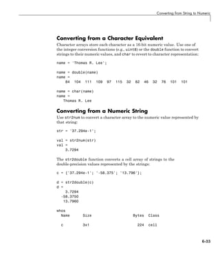
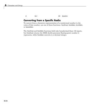
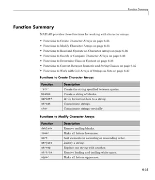
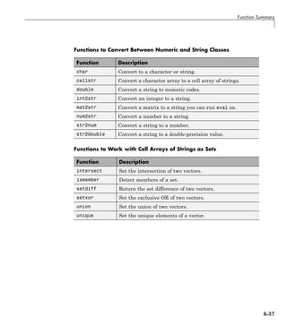

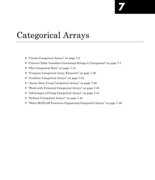
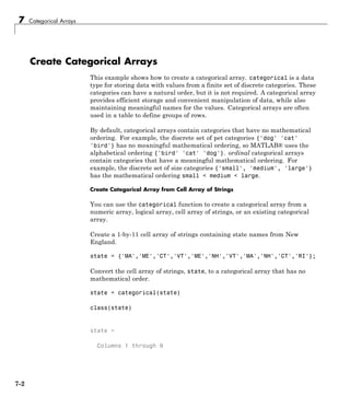
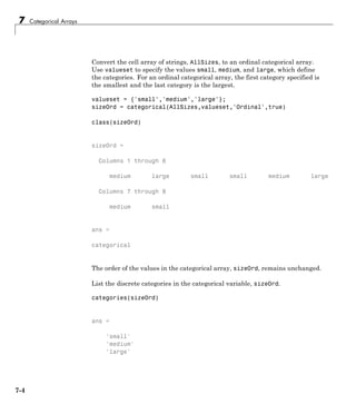
![Create Categorical Arrays
The categories are listed in the specified order to match the mathematical
ordering small < medium < large.
Create Ordinal Categorical Array by Binning Data
Create a vector of 100 integers between 1 and 44.
x = gallery('integerdata',44,[100,1],1);
Use the histc function to create three bins for the data from x. Put all values
between 1 and 15 into bin one, all the values between 15 and 30 into bin two,
and all the values between 30 and 45 into bin three. Each bin includes the left
endpoint, but does not include the right endpoint.
[~,bin] = histc(x,[1,15,30,45]);
bin is a 100-by-1 vector indicating the bin number for each entry from x.
Create and ordinal categorical array, sizeOrd2, where the three bins become
the categories, small, medium, and large.
valueset = 1:3;
catnames = {'small','medium','large'};
sizeOrd2 = categorical(bin,valueset,catnames,'Ordinal',true);
sizeOrd2 is a 100-by-1 ordinal categorical array with three categories, such
that small < medium < large.
Use the summary function to print a summary of the categorical array.
summary(sizeOrd2)
small 33
medium 36
large 31
There are 33 elements in the category small, 36 in the category medium, and
31 in the category large.
7-5](https://image.slidesharecdn.com/matlabprog-220902050722-ff974cdf/85/matlab_prog-pdf-239-320.jpg)
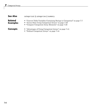
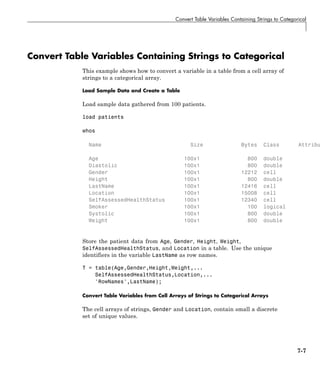
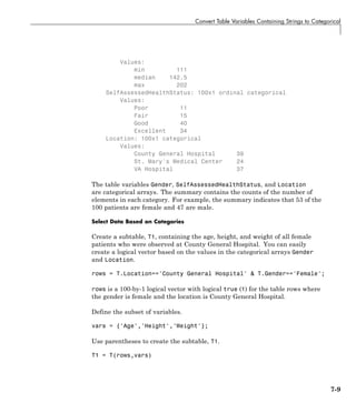
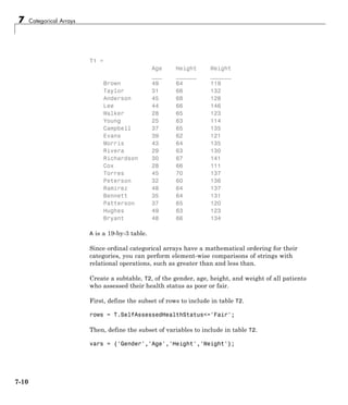
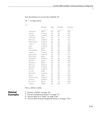

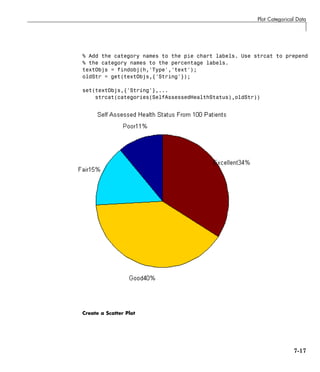
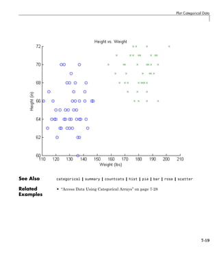
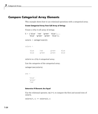
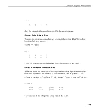
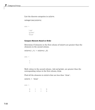
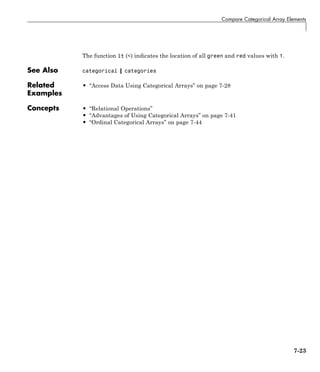
![7 Categorical Arrays
Combine Categorical Arrays
This example shows how to combine two categorical arrays.
Create Categorical Arrays
Create a categorical array, A, containing the preferred lunchtime beverage of
25 students in classroom A.
A = gallery('integerdata',3,[25,1],1);
A = categorical(A,1:3,{'milk' 'water' 'juice'});
A is a 25-by-1 categorical array with three distinct categories: milk, water,
and juice.
Summarize the categorical array, A.
summary(A)
milk 8
water 8
juice 9
Eight students in classroom A prefer milk, eight prefer water, and nine
prefer juice.
Create another categorical array, B, containing the preferences of 28 students
in classroom B.
B = gallery('integerdata',3,[28,1],3);
B = categorical(B,1:3,{'milk' 'water' 'juice'});
B is a 28-by-1 categorical array containing the same categories as A.
Summarize the categorical array, B.
summary(B)
milk 12
water 10
7-24](https://image.slidesharecdn.com/matlabprog-220902050722-ff974cdf/85/matlab_prog-pdf-258-320.jpg)
![Combine Categorical Arrays
juice 6
Twelve students in classroom B prefer milk, ten prefer water, and six prefer
juice.
Concatenate Categorical Arrays
Concatenate the data from classrooms A and B into a single categorical array,
Group1.
Group1 = [A;B];
Summarize the categorical array, Group1
summary(Group1)
milk 20
water 18
juice 15
Group1 is a 53-by-1 categorical array with three categories: milk, water,
and juice.
Create Categorical Array with Different Categories
Create a categorical array, Group2, containing data from 50 students who
were given the additional beverage option of soda.
Group2 = gallery('integerdata',4,[50,1],2);
Group2 = categorical(Group2,1:4,{'juice' 'milk' 'soda' 'water'});
Summarize the categorical array, Group2.
summary(Group2)
juice 18
milk 10
soda 13
water 9
7-25](https://image.slidesharecdn.com/matlabprog-220902050722-ff974cdf/85/matlab_prog-pdf-259-320.jpg)
![7 Categorical Arrays
Group2 is a 50-by-1 categorical array with four categories: juice, milk,
soda, and water.
Concatenate Arrays with Different Categories
Concatenate the data from Group1 and Group2.
students = [Group1;Group2];
Summarize the resulting categorical array, students.
summary(students)
milk 30
water 27
juice 33
soda 13
Concatenation appends the categories exclusive to the second input, soda, to
the end of the list of categories from the first input, milk, water, juice, soda.
Use reordercats to change the order of the categories in the categorical
array, students.
students = reordercats(students,{'juice','milk','water','soda'});
categories(students)
ans =
'juice'
'milk'
'water'
'soda'
Union of Categorical Arrays
7-26](https://image.slidesharecdn.com/matlabprog-220902050722-ff974cdf/85/matlab_prog-pdf-260-320.jpg)
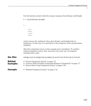
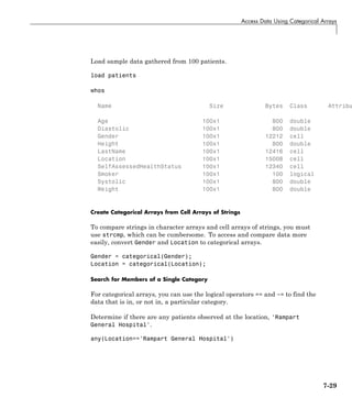
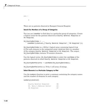
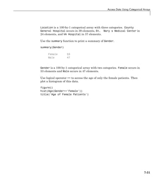
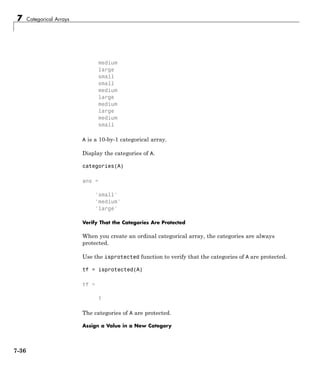
![Work with Protected Categorical Arrays
Try to add the value 'xlarge' to the categorical array, A.
A(2) = 'xlarge'
Error using categorical/subsasgn (line 55)
Cannot add a new category 'xlarge' to this categorical array
because its categories are protected. Use ADDCATEGORIES to
add the new category.
If you try to assign a new value, that does not belong to one of the existing
categories, then MATLAB returns an error.
Use addcats to add a new category for xlarge. Since A is ordinal you must
specify the order for the new category.
A = addcats(A,'xlarge','After','large');
Now, you assign a value for 'xlarge', since it has an existing category.
A(2) = 'xlarge'
A =
medium
xlarge
small
small
medium
large
medium
large
medium
small
A is now a 10-by-1 categorical array with four categories, such that small <
medium < large < xlarge.
Combine Two Ordinal Categorical Arrays
Create another ordinal categorical array, B, containing the sizes of five items.
B = categorical([2;1;1;2;2],1:2,{'xsmall','small'},'Ordinal',true)
7-37](https://image.slidesharecdn.com/matlabprog-220902050722-ff974cdf/85/matlab_prog-pdf-271-320.jpg)
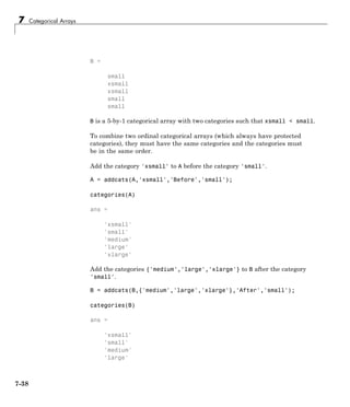
![Work with Protected Categorical Arrays
'xlarge'
The categories of A and B are now the same including their order.
Vertically concatenate A and B.
C = [A;B]
C =
medium
large
small
small
medium
large
medium
large
medium
small
xlarge
small
xsmall
xsmall
small
small
The values from B are appended to the values from A.
List the categories of C.
categories(C)
ans =
'xsmall'
'small'
'medium'
'large'
'xlarge'
7-39](https://image.slidesharecdn.com/matlabprog-220902050722-ff974cdf/85/matlab_prog-pdf-273-320.jpg)
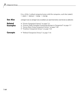
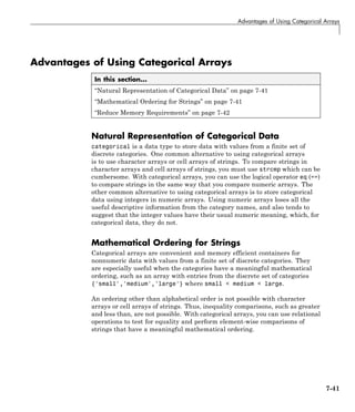
![7 Categorical Arrays
Reduce Memory Requirements
This example shows how to compare the memory required to store data
as a cell array of strings versus a categorical array. Categorical arrays
have categories that are defined as strings, which can be costly to store and
manipulate in a cell array of strings or char array. Categorical arrays store
only one copy of each category name, often reducing the amount of memory
required to store the array.
Create a sample cell array of strings.
state = [repmat({'MA'},25,1);repmat({'NY'},25,1);...
repmat({'CA'},50,1);...
repmat({'MA'},25,1);repmat({'NY'},25,1)];
Display information about the variable state.
whos state
Name Size Bytes Class Attributes
state 150x1 17400 cell
The variable state is a cell array of strings requiring 17,400 bytes of memory.
Convert state to a categorical array.
state = categorical(state);
Display the discrete categories in the variable state.
categories(state)
ans =
'CA'
'MA'
'NY'
7-42](https://image.slidesharecdn.com/matlabprog-220902050722-ff974cdf/85/matlab_prog-pdf-276-320.jpg)
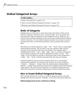
![Ordinal Categorical Arrays
Create an ordinal categorical array, sizes, from a cell array of strings, A.
Use valueset, specified as a vector of unique values, to define the categories
for sizes.
A = {'medium' 'large';'small' 'medium'; 'large' 'small'};
valueset = {'small', 'medium', 'large'};
sizes = categorical(A,valueset,'Ordinal',true)
sizes =
medium large
small medium
large small
sizes is 3-by-2 ordinal categorical array with three categories such that
small < medium < large. The order of the values in valueset becomes
the order of the categories of sizes.
Ordinal Categorical Array from Integers
Create an equivalent categorical array from an array of integers. Use
the values 1, 2, and 3 to define the categories small, medium, and large,
respectively.
A2 = [2 3; 1 2; 3 1];
valueset = 1:3;
catnames = {'small','medium','large'};
sizes2 = categorical(A2,valueset,catnames,'Ordinal',true)
sizes2 =
medium large
small medium
large small
7-45](https://image.slidesharecdn.com/matlabprog-220902050722-ff974cdf/85/matlab_prog-pdf-279-320.jpg)
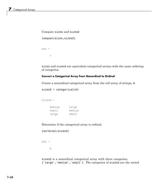
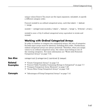

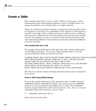
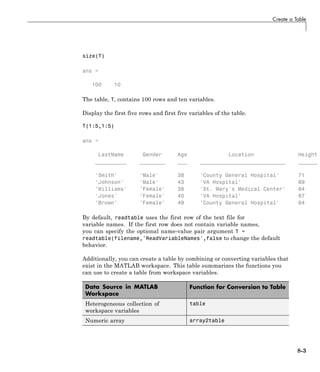
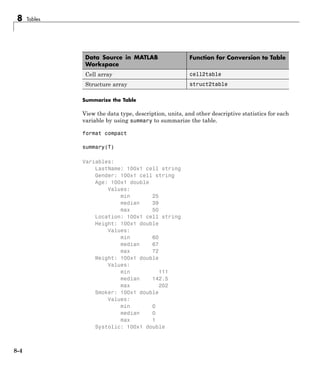
![Create a Table
Values:
min 109
median 122
max 138
Diastolic: 100x1 double
Values:
min 68
median 81.5
max 99
SelfAssessedHealthStatus: 100x1 cell string
The table is heterogeneous. The variables LastName, Gender, Location, and
SelfAssessedHealthStatus are cell arrays of strings, and the other variables
are numeric with a data type of double.
Set the format back to the default.
format
Add Row Names
Tables can be subscripted using parentheses much like ordinary numeric
arrays. But in addition to numeric and logical indices, you can use variable
and row names as indices. Use the unique identifiers in the variable,
LastName, as row names. Then, delete the variable LastName from the table.
T.Properties.RowNames = T.LastName;
T.LastName = [];
Alternatively, you can import the file using readtable with the
'ReadRowNames',true name-value pair argument to indicate that the first
column contains row names.
Return the size of the table.
size(T)
ans =
100 9
8-5](https://image.slidesharecdn.com/matlabprog-220902050722-ff974cdf/85/matlab_prog-pdf-287-320.jpg)
![8 Tables
T contains 100 rows and nine variables. The row and variable names,
respectively, are not included in the size of a table.
Display the first five rows and last four variables of the table.
T(1:5,6:9)
ans =
Smoker Systolic Diastolic SelfAssessedHealthStatus
______ ________ _________ ________________________
Smith 1 124 93 'Excellent'
Johnson 0 109 77 'Fair'
Williams 0 125 83 'Good'
Jones 0 117 75 'Fair'
Brown 0 122 80 'Good'
The elements of the first column in the text file, LastName, are now row
names. Row names and variable names are table properties. You can always
add or change the row names of an existing table by modifying the property
T.Properties.RowNames.
Combine Two Variables into a Single Variable
Create a new variable for blood pressure as a horizontal concatenation of the
two variables Systolic and Diastolic. Then, delete the variables Systolic
and Diastolic.
T.BloodPressure = [T.Systolic T.Diastolic];
T(:,{'Systolic' 'Diastolic'}) = [];
Return the size of the table.
size(T)
ans =
100 8
T contains 100 rows and eight variables. The row and variable names,
respectively, are not included in the size of a table. Furthermore, size
8-6](https://image.slidesharecdn.com/matlabprog-220902050722-ff974cdf/85/matlab_prog-pdf-288-320.jpg)

![Add and Delete Table Rows
Add and Delete Table Rows
This example shows how to add and delete rows in a table. You can also
edit tables using the Variables Editor.
Load Sample Data
Load the sample patients data and create a table, T.
load patients
T = table(LastName,Gender,Age,Height,Weight,Smoker,Systolic,Diastolic);
size(T)
ans =
100 8
The table, T, has 100 rows and 8 variables (columns).
Add Rows by Concatenation
Create a comma-delimited file, morePatients.txt, with the following
additional patient data.
LastName,Gender,Age,Height,Weight,Smoker,Systolic,Diastolic
Abbot,Female,31,65,156,1,128,85
Bailey,Female,38,68,130,0,113,81
Cho,Female,35,61,130,0,124,80
Daniels,Female,48,67,142,1,123,74
Append the rows in the file to the end of the table, T.
T2 = readtable('morePatients.txt');
Tnew = [T;T2];
size(Tnew)
ans =
104 8
8-9](https://image.slidesharecdn.com/matlabprog-220902050722-ff974cdf/85/matlab_prog-pdf-291-320.jpg)
![8 Tables
The table Tnew has 104 rows. In order to vertically concatenate two tables,
both tables must have the same number of variables, with the same variable
names. If the variable names are different, you can directly assign new rows
in a table to rows from another table. For example, T(end+1:end+4,:) = T2.
Add Rows from a Cell Array
If you want to append new rows stored in a cell array, first convert the cell
array to a table, and then concatenate the tables.
cellPatients = {'LastName','Gender','Age','Height','Weight',...
'Smoker','Systolic','Diastolic';
'Edwards','Male',42,70,158,0,116,83;
'Falk','Female',28,62,125,1,120,71};
T2 = cell2table(cellPatients(2:end,:));
T2.Properties.VariableNames = cellPatients(1,:);
Tnew = [Tnew;T2];
size(Tnew)
ans =
106 8
Add Rows from a Structure
You also can append new rows stored in a structure. Convert the structure to
a table, and then concatenate the tables.
structPatients(1,1).LastName = 'George';
structPatients(1,1).Gender = 'Male';
structPatients(1,1).Age = 45;
structPatients(1,1).Height = 76;
structPatients(1,1).Weight = 182;
structPatients(1,1).Smoker = 1;
structPatients(1,1).Systolic = 132;
structPatients(1,1).Diastolic = 85;
structPatients(2,1).LastName = 'Hadley';
structPatients(2,1).Gender = 'Female';
structPatients(2,1).Age = 29;
8-10](https://image.slidesharecdn.com/matlabprog-220902050722-ff974cdf/85/matlab_prog-pdf-292-320.jpg)
![Add and Delete Table Rows
structPatients(2,1).Height = 58;
structPatients(2,1).Weight = 120;
structPatients(2,1).Smoker = 0;
structPatients(2,1).Systolic = 112;
structPatients(2,1).Diastolic = 70;
Tnew = [Tnew;struct2table(structPatients)];
size(Tnew)
ans =
108 8
Omit Duplicate Rows
Use unique to omit any rows in a table that are duplicated.
Tnew = unique(Tnew);
size(Tnew)
ans =
106 8
Two duplicated rows are deleted.
Delete Rows by Row Number
Delete rows 18, 20, and 21 from the table.
Tnew([18,20,21],:) = [];
size(Tnew)
ans =
103 8
The table contains information on 103 patients now.
Delete Rows by Row Name
8-11](https://image.slidesharecdn.com/matlabprog-220902050722-ff974cdf/85/matlab_prog-pdf-293-320.jpg)
![8 Tables
First, specify the variable of identifiers, LastName, as row names. Then,
delete the variable, LastName, from Tnew. Finally, use the row name to index
and delete rows.
Tnew.Properties.RowNames = Tnew.LastName;
Tnew.LastName = [];
Tnew('Smith',:) = [];
size(Tnew)
ans =
102 7
The table now has one less row and one less variable.
Search for Rows To Delete
You also can search for observations in the table. For example, delete rows
for any patients under the age of 30.
toDelete = Tnew.Age<30;
Tnew(toDelete,:) = [];
size(Tnew)
ans =
85 7
The table now has 17 fewer rows.
See Also table | readtable | array2table | cell2table | struct2table | Table
Properties
Related
Examples
• “Add and Delete Table Variables” on page 8-13
• “Clean Messy and Missing Data in Tables” on page 8-18
8-12](https://image.slidesharecdn.com/matlabprog-220902050722-ff974cdf/85/matlab_prog-pdf-294-320.jpg)
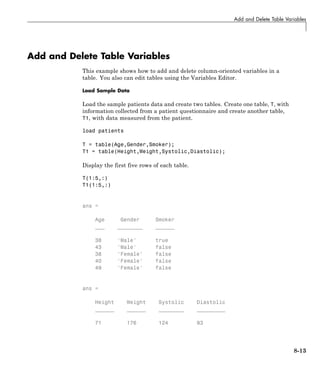
![8 Tables
69 163 109 77
64 131 125 83
67 133 117 75
64 119 122 80
The table T has 100 rows and 3 variables.
The table T1 has 100 rows and 4 variables.
Add Variables by Concatenating Tables
Add variables to the table, T, by horizontally concatenating it with T1.
T = [T T1];
Display the first five rows of the table, T.
T(1:5,:)
ans =
Age Gender Smoker Height Weight Systolic Diastolic
___ ________ ______ ______ ______ ________ _________
38 'Male' true 71 176 124 93
43 'Male' false 69 163 109 77
38 'Female' false 64 131 125 83
40 'Female' false 67 133 117 75
49 'Female' false 64 119 122 80
The table, T, now has 7 variables and 100 rows.
If the tables that you are horizontally concatenating have row names, horzcat
concatenates the tables by matching the row names. Therefore, the tables
must use the same row names, but the row order does not matter.
Add and Delete Variables by Name
8-14](https://image.slidesharecdn.com/matlabprog-220902050722-ff974cdf/85/matlab_prog-pdf-296-320.jpg)
![Add and Delete Table Variables
First create a new variable for blood pressure as a horizontal concatenation
of the two variables Systolic and Diastolic. Then, delete the variables
Systolic and Diastolic by name using dot indexing.
T.BloodPressure = [T.Systolic T.Diastolic];
T.Systolic = [];
T.Diastolic = [];
Alternatively, you can also use parentheses with named indexing to delete the
variables Systolic and Diastolic at once, T(:,{'Systolic','Diastolic'})
= [];.
Display the first five rows of the table, T.
T(1:5,:)
ans =
Age Gender Smoker Height Weight BloodPressure
___ ________ ______ ______ ______ _____________
38 'Male' true 71 176 124 93
43 'Male' false 69 163 109 77
38 'Female' false 64 131 125 83
40 'Female' false 67 133 117 75
49 'Female' false 64 119 122 80
T now has 6 variables and 100 rows.
Add a new variable, BMI, in the table, T, to contain the body mass index for
each patient. BMI is a function of height and weight.
T.BMI = (T.Weight*0.453592)./(T.Height*0.0254).^2;
The operators ./ and .^ in the calculation of BMI indicate element-wise
division and exponentiation, respectively.
8-15](https://image.slidesharecdn.com/matlabprog-220902050722-ff974cdf/85/matlab_prog-pdf-297-320.jpg)
![8 Tables
Display the first five rows of the table, T.
T(1:5,:)
ans =
Age Gender Smoker Height Weight BloodPressure BMI
___ ________ ______ ______ ______ _____________ _____
38 'Male' true 71 176 124 93 24.54
43 'Male' false 69 163 109 77 24.07
38 'Female' false 64 131 125 83 22.48
40 'Female' false 67 133 117 75 20.83
49 'Female' false 64 119 122 80 20.42
T has 100 rows and 7 variables.
Delete Variables by Number
Delete the third variable, Smoker, and the sixth variable, BloodPressure,
from the table.
T(:,[3,6]) = [];
Display the first five rows of the table, T.
T(1:5,:)
ans =
Age Gender Height Weight BMI
___ ________ ______ ______ ______
38 'Male' 71 176 24.547
43 'Male' 69 163 24.071
38 'Female' 64 131 22.486
40 'Female' 67 133 20.831
49 'Female' 64 119 20.426
8-16](https://image.slidesharecdn.com/matlabprog-220902050722-ff974cdf/85/matlab_prog-pdf-298-320.jpg)
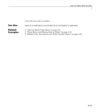
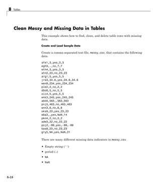
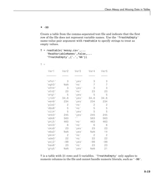
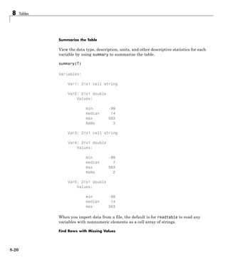
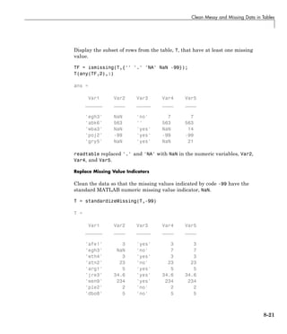
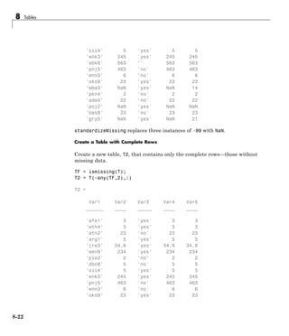
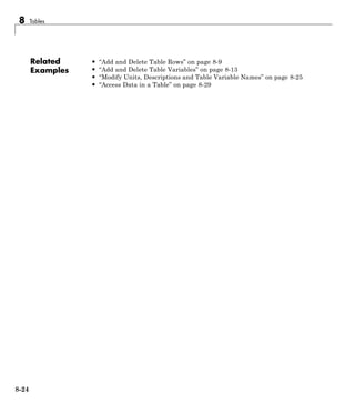
![Modify Units, Descriptions and Table Variable Names
Modify Units, Descriptions and Table Variable Names
This example shows how to access and modify table properties for variable
units, descriptions and names. You also can edit these property values using
the Variables Editor.
Load Sample Data
Load the sample patients data and create a table.
load patients
BloodPressure = [Systolic Diastolic];
T = table(Gender,Age,Height,Weight,Smoker,BloodPressure);
Display the first five rows of the table, T.
T(1:5,:)
ans =
Gender Age Height Weight Smoker BloodPressure
________ ___ ______ ______ ______ _____________
'Male' 38 71 176 true 124 93
'Male' 43 69 163 false 109 77
'Female' 38 64 131 false 125 83
'Female' 40 67 133 false 117 75
'Female' 49 64 119 false 122 80
T has 100 rows and 6 variables.
Add Variable Units
Specify units for each variable in the table by modifying the table property,
VariableUnits. Specify the variable units as a cell array of strings.
T.Properties.VariableUnits = {'' 'Yrs' 'In' 'Lbs' '' ''};
8-25](https://image.slidesharecdn.com/matlabprog-220902050722-ff974cdf/85/matlab_prog-pdf-307-320.jpg)
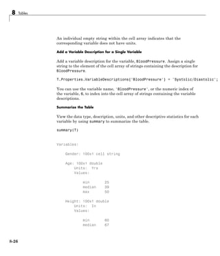
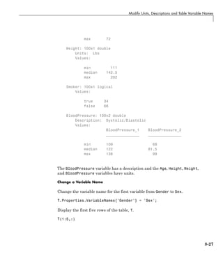
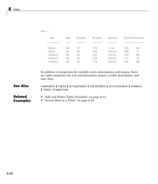
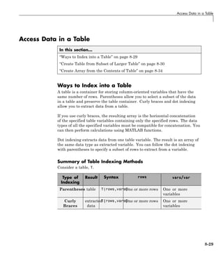
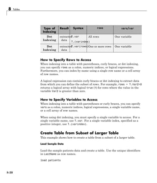
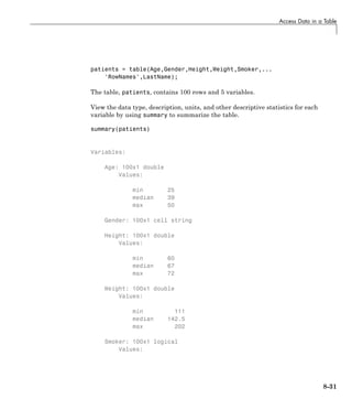
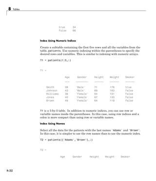
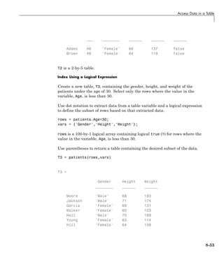
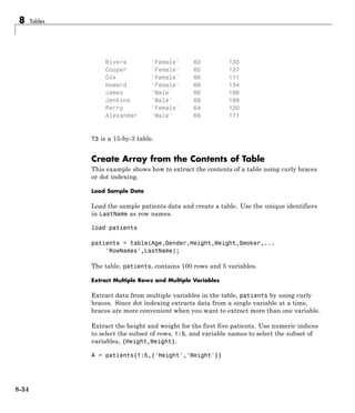
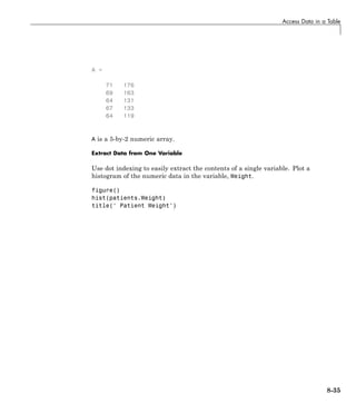
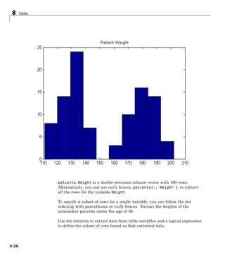
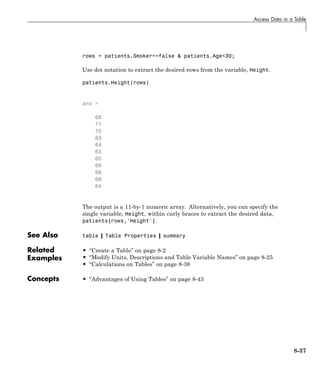
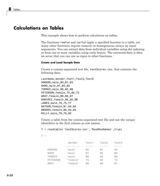
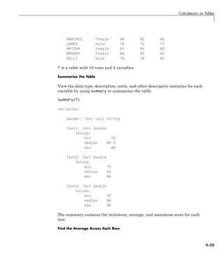
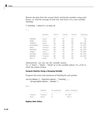
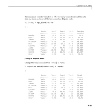
![Advantages of Using Tables
Advantages of Using Tables
In this section...
“Conveniently Store Mixed-Type Data in Single Container” on page 8-43
“Access Data Using Numeric or Named Indexing” on page 8-46
“Use Table Properties to Store Metadata” on page 8-48
Conveniently Store Mixed-Type Data in Single
Container
You can use the table data type to collect mixed-type data and metadata
properties, such as variable name, row names, descriptions, and variable
units, in a single container. Tables are suitable for column-oriented or
tabular data that is often stored as columns in a text file or in a spreadsheet.
For example, you can use a table to store experimental data, with rows
representing different observations and columns representing different
measured variables.
Tables consist of rows and column-oriented variables. Each variable in a
table can have a different data type and a different size, but each variable
must have the same number of rows.
For example, load sample patients data.
load patients
Then, combine the workspace variables, Systolic and Diastolic into a
single BloodPressure variable and convert the workspace variable, Gender,
from a cell array of strings to a categorical array.
BloodPressure = [Systolic Diastolic];
Gender = categorical(Gender);
whos('Gender','Age','Smoker','BloodPressure')
Name Size Bytes Class Attributes
Age 100x1 800 double
8-43](https://image.slidesharecdn.com/matlabprog-220902050722-ff974cdf/85/matlab_prog-pdf-325-320.jpg)
![8 Tables
BloodPressure 100x2 1600 double
Gender 100x1 550 categorical
Smoker 100x1 100 logical
The variables Age, BloodPressure, Gender, and Smoker have varying data
types and are candidates to store in a table since they all have the same
number of rows, 100.
Now, create a table from the variables and display the first five rows.
T = table(Gender,Age,Smoker,BloodPressure);
T(1:5,:)
ans =
Gender Age Smoker BloodPressure
______ ___ ______ _______________
Male 38 true 124 93
Male 43 false 109 77
Female 38 false 125 83
Female 40 false 117 75
Female 49 false 122 80
The table displays in a tabular format with the variable names at the top.
Each variable in a table is a single data type. For example, if you add a new
row to the table, MATLAB forces consistency of the data type between the
new data and the corresponding table variables. If you try to add information
for a new patient where the first column contains the patient’s age instead of
gender, you receive an error.
T(end+1,:) = {37,{'Female'},true,[130 84]}
Error using table/subsasgnParens (line 200)
Invalid RHS for assignment to a categorical array.
Error in table/subsasgn (line 61)
t = subsasgnParens(t,s,b,creating);
8-44](https://image.slidesharecdn.com/matlabprog-220902050722-ff974cdf/85/matlab_prog-pdf-326-320.jpg)
![Advantages of Using Tables
The error occurs because MATLAB cannot assign numeric data to the
categorical array, Gender.
For comparison of tables with structures, consider the structure array,
StructArray, that is equivalent to the table, T.
StructArray = table2struct(T)
'StructArray =
101x1 struct array with fields:
Gender
Age
Smoker
BloodPressure
Structure arrays organize records using named fields. Each field’s value can
have a different data type or size. Now, display the named fields for the first
element of StructArray.
StructArray(1)
ans =
Gender: [1x1 categorical]
Age: 38
Smoker: 1
BloodPressure: [124 93]
Fields in a structure array are analogous to variables in a table. However,
unlike with tables, you cannot enforce homogeneity within a field. For
example, you can have some values of S.Gender that are categorical array
elements, 'Male' or 'Female', others that are strings, 'Male' or 'Female',
and others that are integers, 0 or 1.
Now consider the same data stored in a scalar structure, with four fields each
containing one variable from the table.
ScalarStruct = struct(...
'Gender',{Gender},...
8-45](https://image.slidesharecdn.com/matlabprog-220902050722-ff974cdf/85/matlab_prog-pdf-327-320.jpg)
![8 Tables
'Age',Age,...
'Smoker',Smoker,...
'BloodPressure',BloodPressure)
ScalarStruct =
Gender: [100x1 categorical]
Age: [100x1 double]
Smoker: [100x1 logical]
BloodPressure: [100x2 double]
Unlike with tables, you cannot enforce that the data is rectangular. For
example, the field ScalarStruct.Age can be a different length than the
other fields.
A table allows you to maintain the rectangular structure (like a structure
array) and enforce homogeneity of variables (like fields in a scalar structure).
Although cell arrays do not have named fields, they have many of the
same disadvantages as structure arrays and scalar structures. If you have
rectangular data that is homogeneous in each variable, consider using a
table. Then you can use numeric or named indexing, and you can use table
properties to store metadata.
Access Data Using Numeric or Named Indexing
You can index into a table using parentheses, curly braces, or dot indexing.
Parentheses allow you to select a subset of the data in a table and preserve
the table container. Curly braces and dot indexing allow you to extract data
from a table. Within each table indexing method, you can specify the rows or
variables to access by name or by numeric index.
Consider the sample table from above. Each row in the table, T, represents
a different patient. The workspace variable, LastName, contains unique
identifiers for the 100 rows. Add row names to the table by setting the
RowNames property to LastName and display the first five rows of the updated
table.
T.Properties.RowNames = LastName;
T(1:5,:)
ans =
8-46](https://image.slidesharecdn.com/matlabprog-220902050722-ff974cdf/85/matlab_prog-pdf-328-320.jpg)
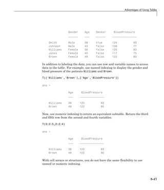
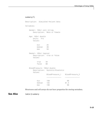
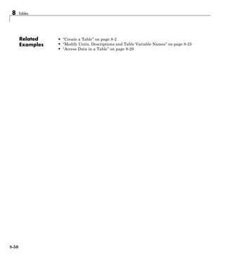
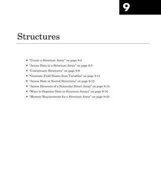
![9 Structures
Create a Structure Array
This example shows how to create a structure array. A structure is a data
type that groups related data using data containers called fields. Each field
can contain data of any type or size.
Store a patient record in a scalar structure with fields name, billing, and
test.
patient.name = 'John Doe';
patient.billing = 127.00;
patient.test = [79, 75, 73; 180, 178, 177.5; 220, 210, 205];
patient
patient =
name: 'John Doe'
billing: 127
test: [3x3 double]
Add records for other patients to the array by including subscripts after the
array name.
patient(2).name = 'Ann Lane';
patient(2).billing = 28.50;
patient(2).test = [68, 70, 68; 118, 118, 119; 172, 170, 169];
patient
patient =
1x2 struct array with fields:
9-2](https://image.slidesharecdn.com/matlabprog-220902050722-ff974cdf/85/matlab_prog-pdf-334-320.jpg)
![Create a Structure Array
name
billing
test
Each patient record in the array is a structure of class struct. An array of
structures is often referred to as a struct array. Like other MATLAB arrays, a
struct array can have any dimensions.
A struct array has the following properties:
• All structs in the array have the same number of fields.
• All structs have the same field names.
• Fields of the same name in different structs can contain different types
or sizes of data.
Any unspecified fields for new structs in the array contain empty arrays.
patient(3).name = 'New Name';
patient(3)
ans =
name: 'New Name'
billing: []
test: []
Access data in the structure array to find how much the first patient owes,
and to create a bar graph of his test results.
amount_due = patient(1).billing
bar(patient(1).test)
title(['Test Results for ', patient(1).name])
amount_due =
9-3](https://image.slidesharecdn.com/matlabprog-220902050722-ff974cdf/85/matlab_prog-pdf-335-320.jpg)
![Access Data in a Structure Array
Access Data in a Structure Array
This example shows how to access the contents of a structure array. To
run the code in this example, load several variables into a scalar (1-by-1)
structure named S.
S = load('clown.mat')
S =
X: [200x320 double]
map: [81x3 double]
caption: [2x1 char]
The variables from the file (X, caption, and map) are now fields in the struct.
Access the data using dot notation of the form structName.fieldName. For
example, pass the numeric data in field X to the image function:
image(S.X)
colormap(S.map)
9-5](https://image.slidesharecdn.com/matlabprog-220902050722-ff974cdf/85/matlab_prog-pdf-337-320.jpg)
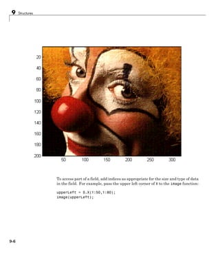
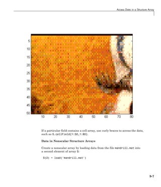
![Concatenate Structures
Concatenate Structures
This example shows how to concatenate structure arrays using the []
operator. To concatenate structures, they must have the same set of fields,
but the fields do not need to contain the same sizes or types of data.
Create scalar (1-by-1) structure arrays struct1 and struct2, each with fields
a and b:
struct1.a = 'first';
struct1.b = [1,2,3];
struct2.a = 'second';
struct2.b = rand(5);
Just as concatenating two scalar values such as [1, 2] creates a 1-by-2
numeric array, concatenating struct1 and struct2,
combined = [struct1, struct2]
creates a 1-by-2 structure array:
combined =
1x2 struct array with fields:
a
b
When you want to access the contents of a particular field, specify the index of
the structure in the array. For example, access field a of the first structure:
combined(1).a
This code returns
ans =
first
Concatenation also applies to nonscalar structure arrays. For example, create
a 2-by-2 structure array named new:
new(1,1).a = 1; new(1,1).b = 10;
new(1,2).a = 2; new(1,2).b = 20;
9-9](https://image.slidesharecdn.com/matlabprog-220902050722-ff974cdf/85/matlab_prog-pdf-341-320.jpg)
![9 Structures
new(2,1).a = 3; new(2,1).b = 30;
new(2,2).a = 4; new(2,2).b = 40;
Because the 1-by-2 structure combined and the 2-by-2 structure new both have
two columns, you can concatenate them vertically with a semicolon separator:
larger = [combined; new]
This code returns a 3-by-2 structure array,
larger =
3x2 struct array with fields:
a
b
where, for example,
larger(2,1).a =
1
For related information, see:
• “Creating and Concatenating Matrices”
• “Access Data in a Structure Array” on page 9-5
• “Access Elements of a Nonscalar Struct Array” on page 9-14
9-10](https://image.slidesharecdn.com/matlabprog-220902050722-ff974cdf/85/matlab_prog-pdf-342-320.jpg)
![Generate Field Names from Variables
Generate Field Names from Variables
This example shows how to derive a structure field name at run time from a
variable or expression. The general syntax is
structName.(dynamicExpression)
where dynamicExpression is a variable or expression that returns a character
or string. Field names that you reference with expressions are called dynamic
field names.
For example, create a field name from the current date:
currentDate = datestr(now,'mmmdd');
myStruct.(currentDate) = [1,2,3]
If the current date reported by your system is February 29, then this code
assigns data to a field named Feb29:
myStruct =
Feb29: [1 2 3]
Field names, like variable names, must begin with a letter, can contain
letters, digits, or underscore characters, and are case sensitive. To avoid
potential conflicts, do not use the names of existing variables or functions as
field names. For more information, see “Variable Names” on page 1-8.
9-11](https://image.slidesharecdn.com/matlabprog-220902050722-ff974cdf/85/matlab_prog-pdf-343-320.jpg)
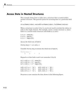
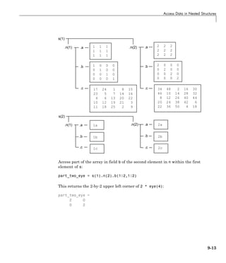
![9 Structures
Access Elements of a Nonscalar Struct Array
This example shows how to access and process data from multiple elements of
a nonscalar structure array:
Create a 1-by-3 structure s with field f:
s(1).f = 1;
s(2).f = 'two';
s(3).f = 3 * ones(3);
Although each structure in the array must have the same number of fields
and the same field names, the contents of the fields can be different types and
sizes. When you refer to field f for multiple elements of the structure array,
such as
s(1:3).f
or
s.f
MATLAB returns the data from the elements in a comma-separated list,
which displays as follows:
ans =
1
ans =
two
ans =
3 3 3
3 3 3
3 3 3
You cannot assign the list to a single variable with the syntax v = s.f
because the fields can contain different types of data. However, you can
assign the list items to the same number of variables, such as
[v1, v2, v3] = s.f;
9-14](https://image.slidesharecdn.com/matlabprog-220902050722-ff974cdf/85/matlab_prog-pdf-346-320.jpg)
![Access Elements of a Nonscalar Struct Array
or assign to elements of a cell array, such as
c = {s.f};
If all of the fields contain the same type of data and can form a hyperrectangle,
you can concatenate the list items. For example, create a structure nums with
scalar numeric values in field f, and concatenate the data from the fields:
nums(1).f = 1;
nums(2).f = 2;
nums(3).f = 3;
allNums = [nums.f]
This code returns
allNums =
1 2 3
If you want to process each element of an array with the same operation, use
the arrayfun function. For example, count the number of elements in field
f of each struct in array s:
numElements = arrayfun(@(x) numel(x.f), s)
The syntax @(x) creates an anonymous function. This code calls the numel
function for each element of array s, such as numel(s(1).f), and returns
numElements =
1 3 9
For related information, see:
• “Comma-Separated Lists” on page 2-61
• “Anonymous Functions” on page 17-23
9-15](https://image.slidesharecdn.com/matlabprog-220902050722-ff974cdf/85/matlab_prog-pdf-347-320.jpg)
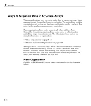
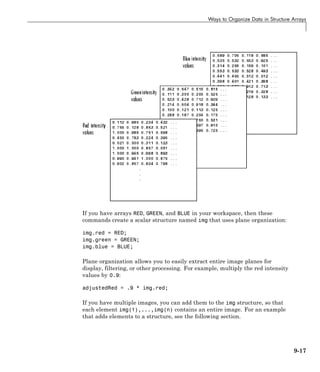
![9 Structures
Element-by-Element Organization
Consider a database with patient information. Each record contains data for
the patient’s name, test results, and billing amount.
These statements create an element in a structure array named patient:
patient(1).name = 'John Doe';
patient(1).billing = 127.00;
patient(1).test = [79, 75, 73; 180, 178, 177.5; 220, 210, 205];
Additional patients correspond to new elements in the structure. For example,
add an element for a second patient:
patient(2).name = 'Ann Lane';
patient(2).billing = 28.50;
patient(2).test = [68, 70, 68; 118, 118, 119; 172, 170, 169];
Element-by-element organization supports simple indexing to access data for
a particular patient. For example, find the average of the first patient’s test
results, calculating by rows (dimension 2) rather than by columns:
aveResultsDoe = mean(patient(1).test,2)
This code returns
aveResultsDoe =
9-18](https://image.slidesharecdn.com/matlabprog-220902050722-ff974cdf/85/matlab_prog-pdf-350-320.jpg)
![9 Structures
Memory Requirements for a Structure Array
Structure arrays do not require completely contiguous memory. However,
each field requires contiguous memory, as does the header that MATLAB
creates to describe the array. For very large arrays, incrementally increasing
the number of fields or the number of elements in a field results in Out of
Memory errors.
Allocate memory for the contents by assigning initial values with the struct
function, such as
newStruct(1:25,1:50) = struct('a',ones(20),'b',zeros(30),'c',rand(40));
This code creates and populates a 25-by-50 structure array S with fields a,
b, and c.
If you prefer not to assign initial values, you can initialize a structure array
by assigning empty arrays to each field of the last element in the structure
array, such as
newStruct(25,50).a = [];
newStruct(25,50).b = [];
newStruct(25,50).c = [];
or, equivalently,
newStruct(25,50) = struct('a',[],'b',[],'c',[]);
However, in this case, MATLAB only allocates memory for the header, and
not for the contents of the array.
For more information, see:
• “Preallocating Memory”
• “Memory Allocation” on page 26-2
9-20](https://image.slidesharecdn.com/matlabprog-220902050722-ff974cdf/85/matlab_prog-pdf-352-320.jpg)

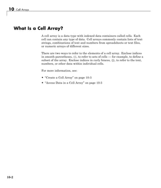
![Create a Cell Array
Create a Cell Array
This example shows how to create a cell array using the {} operator or the
cell function.
When you have data to put into a cell array, create the array using the cell
array construction operator, {}:
myCell = {1, 2, 3;
'text', rand(5,10,2), {11; 22; 33}}
Like all MATLAB arrays, cell arrays are rectangular, with the same number
of cells in each row. myCell is a 2-by-3 cell array:
myCell =
[ 1] [ 2] [ 3]
'text' [5x10x2 double] {3x1 cell}
You also can use the {} operator to create an empty 0-by-0 cell array,
C = {}
If you plan to add values to a cell array over time or in a loop, you can create
an empty n-dimensional array using the cell function:
emptyCell = cell(3,4,2)
emptyCell is a 3-by-4-by-2 cell array, where each cell contains an empty
array, []:
emptyCell(:,:,1) =
[] [] [] []
[] [] [] []
[] [] [] []
emptyCell(:,:,2) =
[] [] [] []
[] [] [] []
[] [] [] []
10-3](https://image.slidesharecdn.com/matlabprog-220902050722-ff974cdf/85/matlab_prog-pdf-355-320.jpg)
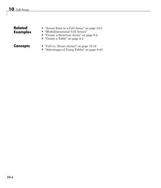
![Access Data in a Cell Array
Access Data in a Cell Array
This example shows how to read and write data to and from a cell array. To
run the code in this example, create a 2-by-3 cell array of text and numeric
data:
C = {'one', 'two', 'three';
1, 2, 3};
There are two ways to refer to the elements of a cell array. Enclose indices
in smooth parentheses, (), to refer to sets of cells—for example, to define a
subset of the array. Enclose indices in curly braces, {}, to refer to the text,
numbers, or other data within individual cells.
Cell Indexing with Smooth Parentheses, ()
Cell array indices in smooth parentheses refer to sets of cells. For example,
the command
upperLeft = C(1:2,1:2)
creates a 2-by-2 cell array:
upperLeft =
'one' 'two'
[ 1] [ 2]
Update sets of cells by replacing them with the same number of cells. For
example, the statement
C(1,1:3) = {'first','second','third'}
replaces the cells in the first row of C with an equivalent-sized (1-by-3) cell
array:
C =
'first' 'second' 'third'
[ 1] [ 2] [ 3]
If cells in your array contain numeric data, you can convert the cells to a
numeric array using the cell2mat function:
10-5](https://image.slidesharecdn.com/matlabprog-220902050722-ff974cdf/85/matlab_prog-pdf-357-320.jpg)
![10 Cell Arrays
numericCells = C(2,1:3)
numericVector = cell2mat(numericCells)
numericCells is a 1-by-3 cell array, but numericVector is a 1-by-3 array of
type double:
numericCells =
[1] [2] [3]
numericVector =
1 2 3
Content Indexing with Curly Braces, {}
Access the contents of cells—the numbers, text, or other data within the
cells—by indexing with curly braces. For example, the command
last = C{2,3}
creates a numeric variable of type double, because the cell contains a double
value:
last =
3
Similarly, this command
C{2,3} = 300
replaces the contents of the last cell of C with a new, numeric value:
C =
'first' 'second' 'third'
[ 1] [ 2] [ 300]
When you access the contents of multiple cells, such as
C{1:2,1:2}
MATLAB creates a comma-separated list. Because each cell can contain
a different type of data, you cannot assign this list to a single variable.
However, you can assign the list to the same number of variables as cells.
MATLAB assigns to the variables in column order. For example,
10-6](https://image.slidesharecdn.com/matlabprog-220902050722-ff974cdf/85/matlab_prog-pdf-358-320.jpg)
![Access Data in a Cell Array
[r1c1, r2c1, r1c2, r2c2] = C{1:2,1:2}
returns
r1c1 =
first
r2c1 =
1
r1c2 =
second
r2c2 =
2
If each cell contains the same type of data, you can create a single variable
by applying the array concatenation operator, [], to the comma-separated
list. For example,
nums = [C{2,:}]
returns
nums =
1 2 300
For more information, see:
• “Multilevel Indexing to Access Parts of Cells” on page 10-20
• “Comma-Separated Lists” on page 2-61
10-7](https://image.slidesharecdn.com/matlabprog-220902050722-ff974cdf/85/matlab_prog-pdf-359-320.jpg)
![10 Cell Arrays
Add Cells to a Cell Array
This example shows how to add cells to a cell array.
Create a 1-by-3 cell array:
C = {1, 2, 3};
Assign data to a cell outside the current dimensions:
C{4,4} = 44
MATLAB expands the cell array to a rectangle that includes the specified
subscripts. Any intervening cells contain empty arrays:
C =
[1] [2] [3] []
[] [] [] []
[] [] [] []
[] [] [] [44]
Add cells without specifying a value by assigning an empty array as the
contents of a cell:
C{5,5} = []
C is now a 5-by-5 cell array:
C =
[1] [2] [3] [] []
[] [] [] [] []
[] [] [] [] []
[] [] [] [44] []
[] [] [] [] []
For related examples, see:
• “Access Data in a Cell Array” on page 10-5
• “Combine Cell Arrays” on page 10-10
• “Delete Data from a Cell Array” on page 10-9
10-8](https://image.slidesharecdn.com/matlabprog-220902050722-ff974cdf/85/matlab_prog-pdf-360-320.jpg)
![Delete Data from a Cell Array
Delete Data from a Cell Array
This example shows how to remove data from individual cells, and how to
delete entire cells from a cell array. To run the code in this example, create a
3-by-3 cell array:
C = {1, 2, 3; 4, 5, 6; 7, 8, 9};
Delete the contents of a particular cell by assigning an empty array to the
cell, using curly braces for content indexing, {}:
C{2,2} = []
This code returns
C =
[1] [2] [3]
[4] [] [6]
[7] [8] [9]
Delete sets of cells using standard array indexing with smooth parentheses,
(). For example, this command
C(2,:) = []
removes the second row of C:
C =
[1] [2] [3]
[7] [8] [9]
For related examples, see:
• “Add Cells to a Cell Array” on page 10-8
• “Access Data in a Cell Array” on page 10-5
10-9](https://image.slidesharecdn.com/matlabprog-220902050722-ff974cdf/85/matlab_prog-pdf-361-320.jpg)
![10 Cell Arrays
Combine Cell Arrays
This example shows how to combine cell arrays by concatenation or nesting.
To run the code in this example, create several cell arrays with the same
number of columns:
C1 = {1, 2, 3};
C2 = {'A', 'B', 'C'};
C3 = {10, 20, 30};
Concatenate cell arrays with the array concatenation operator, []. In this
example, vertically concatenate the cell arrays by separating them with
semicolons:
C4 = [C1; C2; C3]
C4 is a 3-by-3 cell array:
C4 =
[ 1] [ 2] [ 3]
'A' 'B' 'C'
[10] [20] [30]
Create a nested cell array with the cell array construction operator, {}:
C5 = {C1; C2; C3}
C5 is a 3-by-1 cell array, where each cell contains a cell array:
C5 =
{1x3 cell}
{1x3 cell}
{1x3 cell}
For more information, see “Concatenating Matrices”.
10-10](https://image.slidesharecdn.com/matlabprog-220902050722-ff974cdf/85/matlab_prog-pdf-362-320.jpg)
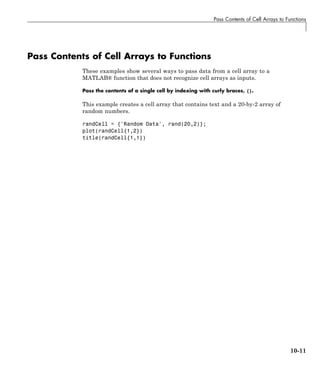
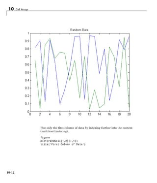
![Pass Contents of Cell Arrays to Functions
Combine numeric data from multiple cells using the cell2mat function.
This example creates a 5-by-2 cell array that stores temperature data for
three cities, and plots the temperatures for each city by date.
temperature(1,:) = {'01-Jan-2010', [45, 49, 0]};
temperature(2,:) = {'03-Apr-2010', [54, 68, 21]};
temperature(3,:) = {'20-Jun-2010', [72, 85, 53]};
temperature(4,:) = {'15-Sep-2010', [63, 81, 56]};
temperature(5,:) = {'31-Dec-2010', [38, 54, 18]};
10-13](https://image.slidesharecdn.com/matlabprog-220902050722-ff974cdf/85/matlab_prog-pdf-365-320.jpg)
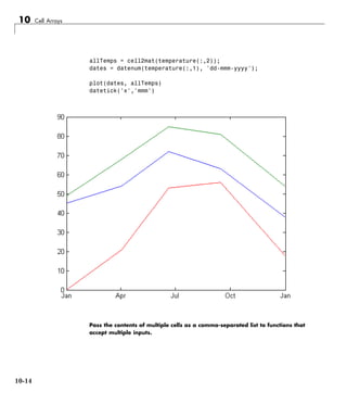
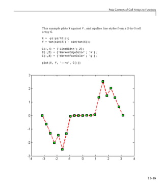
![Preallocate Memory for a Cell Array
Preallocate Memory for a Cell Array
This example shows how to initialize and allocate memory for a cell array.
Cell arrays do not require completely contiguous memory. However, each cell
requires contiguous memory, as does the cell array header that MATLAB
creates to describe the array. For very large arrays, incrementally increasing
the number of cells or the number of elements in a cell results in Out of
Memory errors.
Initialize a cell array by calling the cell function, or by assigning to the last
element. For example, these statements are equivalent:
C = cell(25,50);
C{25,50} = [];
MATLAB creates the header for a 25-by-50 cell array. However, MATLAB
does not allocate any memory for the contents of each cell.
For more information, see:
• “Preallocating Memory”
• “Memory Allocation” on page 26-2
10-17](https://image.slidesharecdn.com/matlabprog-220902050722-ff974cdf/85/matlab_prog-pdf-369-320.jpg)
![10 Cell Arrays
Cell vs. Struct Arrays
This example compares cell and structure arrays, and shows how to store data
in each type of array. Both cell and structure arrays allow you to store data
of different types and sizes.
Structure Arrays
Structure arrays contain data in fields that you access by name.
For example, store patient records in a structure array.
patient(1).name = 'John Doe';
patient(1).billing = 127.00;
patient(1).test = [79, 75, 73; 180, 178, 177.5; 220, 210, 205];
patient(2).name = 'Ann Lane';
patient(2).billing = 28.50;
patient(2).test = [68, 70, 68; 118, 118, 119; 172, 170, 169];
Create a bar graph of the test results for each patient.
numPatients = numel(patient);
for p = 1:numPatients
figure
bar(patient(p).test)
title(patient(p).name)
end
Cell Arrays
Cell arrays contain data in cells that you access by numeric indexing.
Common applications of cell arrays include storing lists of text strings and
storing heterogeneous data from spreadsheets.
For example, store temperature data for three cities over time in a cell array.
temperature(1,:) = {'01-Jan-2010', [45, 49, 0]};
temperature(2,:) = {'03-Apr-2010', [54, 68, 21]};
temperature(3,:) = {'20-Jun-2010', [72, 85, 53]};
temperature(4,:) = {'15-Sep-2010', [63, 81, 56]};
10-18](https://image.slidesharecdn.com/matlabprog-220902050722-ff974cdf/85/matlab_prog-pdf-370-320.jpg)
![Cell vs. Struct Arrays
temperature(5,:) = {'31-Dec-2010', [38, 54, 18]};
Plot the temperatures for each city by date.
allTemps = cell2mat(temperature(:,2));
dates = datenum(temperature(:,1), 'dd-mmm-yyyy');
plot(dates,allTemps)
datetick('x','mmm')
Other Container Arrays
Struct and cell arrays are the most commonly used containers for storing
heterogeneous data. Tables are convenient for storing heterogeneous
column-oriented or tabular data. Alternatively, use map containers, or create
your own class.
See Also cell | containers.Map | table | struct
Related
Examples
• “Access Data in a Cell Array” on page 10-5
• “Access Data in a Structure Array” on page 9-5
• “Access Data in a Table” on page 8-29
Concepts • “Advantages of Using Tables” on page 8-43
10-19](https://image.slidesharecdn.com/matlabprog-220902050722-ff974cdf/85/matlab_prog-pdf-371-320.jpg)
![10 Cell Arrays
Multilevel Indexing to Access Parts of Cells
This example explains techniques for accessing data in arrays stored within
cells of cell arrays. To run the code in this example, create a sample cell array:
myNum = [1, 2, 3];
myCell = {'one', 'two'};
myStruct.Field1 = ones(3);
myStruct.Field2 = 5*ones(5);
C = {myNum, 100*myNum;
myCell, myStruct};
Access the complete contents of a particular cell using curly braces, {}. For
example,
C{1,2}
returns the numeric vector from that cell:
ans =
100 200 300
Access part of the contents of a cell by appending indices, using syntax that
matches the data type of the contents. For example:
• Enclose numeric indices in smooth parentheses. For example, C{1,1}
returns the 1-by-3 numeric vector, [1, 2, 3]. Access the second element
of that vector with the syntax
C{1,1}(1,2)
which returns
ans =
2
• Enclose cell array indices in curly braces. For example, C{2,1} returns the
cell array {'one', 'two'}. Access the contents of the second cell within
that cell array with the syntax
C{2,1}{1,2}
10-20](https://image.slidesharecdn.com/matlabprog-220902050722-ff974cdf/85/matlab_prog-pdf-372-320.jpg)
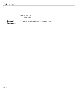

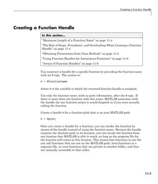
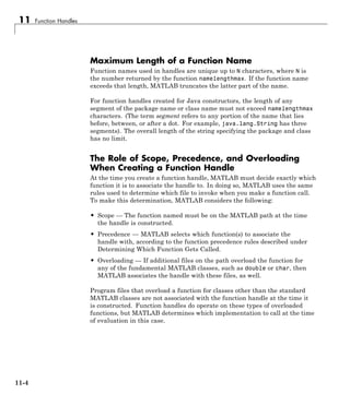
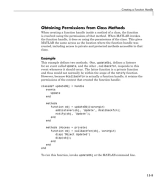
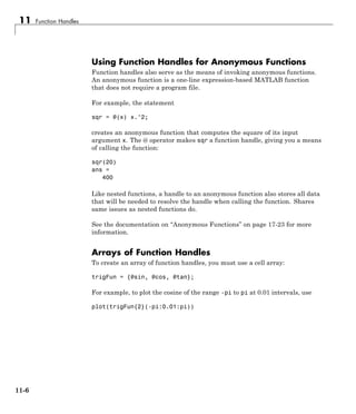
![Calling a Function Using Its Handle
Calling a Function Using Its Handle
In this section...
“Calling Syntax” on page 11-7
“Calling a Function with Multiple Outputs” on page 11-8
“Returning a Handle for Use Outside of a Function File” on page 11-8
“Example — Using Function Handles in Optimization” on page 11-9
Function handles can give you access to functions you might not be able to
execute. For instance, with a handle you can call a function even if it is no
longer on your MATLAB path. You can also call a local function from outside
of the file that defines that function.
Calling Syntax
The syntax for calling a function using a function handle is the same as that
used when calling the function directly. For example, if you call function
myFun like this:
[out1, out2, ...] = myFun(in1, in2, ...);
then you would call it using a handle in the same way, but using the handle
name instead:
fHandle = @myFun;
[out1, out2, ...] = fHandle(in1, in2, ...);
There is one small difference. If the function being called takes no input
arguments, then you must call the function with empty parentheses placed
after the handle name. If you use only the handle name, MATLAB just
identifies the name of the function:
% This identifies the handle. % This invokes the function.
fHandle = @computer; fHandle = @computer;
fHandle fHandle()
ans = ans =
@computer PCWIN
11-7](https://image.slidesharecdn.com/matlabprog-220902050722-ff974cdf/85/matlab_prog-pdf-381-320.jpg)
![11 Function Handles
Calling a Function with Multiple Outputs
The example below returns multiple values from a call to an anonymous
function. Create anonymous function f that locates the nonzero elements of
an array, and returns the row, column, and value of each element in variables
row, col, and val:
f = @(X)find(X);
Call the function on matrix m using the function handle f. Because the
function uses the MATLAB find function which returns up to three outputs,
you can specify from 0 to 3 outputs in the call:
m = [3 2 0; -5 0 7; 0 0 1]
m =
3 2 0
-5 0 7
0 0 1
[row col val] = f(m);
val
val =
3
-5
2
7
1
Returning a Handle for Use Outside of a Function File
As stated previously, you can use function handles to call a function that may
otherwise be hidden or out of scope. This example function getHandle returns
a function handle fHandle to a caller that is outside of the file:
function fHandle = getHandle
fHandle = @subFun;
function res = subFun(t1, t2, varargin);
...
11-8](https://image.slidesharecdn.com/matlabprog-220902050722-ff974cdf/85/matlab_prog-pdf-382-320.jpg)
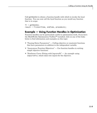
![11 Function Handles
Preserving Data from the Workspace
In this section...
“Preserving Data with Anonymous Functions” on page 11-10
“Preserving Data with Nested Functions” on page 11-11
Both anonymous functions and nested functions make use of variable data
that is stored outside the body of the function itself. For example, the
anonymous function shown here uses two variables: X and K. You pass the X
variable into the anonymous function whenever you invoke the function. The
value for K however is taken from the currently active workspace:
K = 200;
fAnon = @(X)K * X;
fAnon([2.54 1.43 0.68 1.90 1.02 2.13]);
What would happen if you tried to invoke this function after you cleared K
from the workspace? Or if you saved the anonymous function to a .mat file
and then loaded it into an entirely separate computing environment where
K is not defined?
The answer is that MATLAB stores any values needed by an anonymous (or
nested) function within the handle itself. It does this at the time you construct
the handle. This does not include values from the argument list as these
values get passed in whenever you call the function.
Preserving Data with Anonymous Functions
If you create an anonymous function at the MATLAB command window, that
function has access to the workspace of your current MATLAB session. If you
create the function inside of another function, then it has access to the outer
function’s workspace. Either way, if your anonymous function depends upon
variables from an outside workspace, then MATLAB stores the variables and
their values within the function handle at the time the handle is created.
This example puts a 3-by-5 matrix into the base workspace, and then creates a
function handle to an anonymous function that requires access to the matrix.
11-10](https://image.slidesharecdn.com/matlabprog-220902050722-ff974cdf/85/matlab_prog-pdf-384-320.jpg)
![Preserving Data from the Workspace
Create matrix A and anonymous function testAnon:
A = magic(5); A(4:5,:) = []
A =
17 24 1 8 15
23 5 7 14 16
4 6 13 20 22
testAnon = @(x)x * A; % Anonymous function
Call the anonymous function via its handle, passing in a multiplier value.
This multiplies all elements by 5.2:
testAnon(5.2)
ans =
88.4000 124.8000 5.2000 41.6000 78.0000
119.6000 26.0000 36.4000 72.8000 83.2000
20.8000 31.2000 67.6000 104.0000 114.4000
Clear variable A from the base workspace and verify that this action has no
effect on the output of the anonymous function:
clear A
testAnon(5.2)
ans =
88.4000 124.8000 5.2000 41.6000 78.0000
119.6000 26.0000 36.4000 72.8000 83.2000
20.8000 31.2000 67.6000 104.0000 114.4000
This works because the variable A and its value at the time the anonymous
function is created is preserved within the function handle that also provides
access to the anonymous function. See “Variables in the Expression” on page
17-24 for more information.
Preserving Data with Nested Functions
Nested functions are similar to anonymous functions in their ability to
preserve workspace data needed by a function handle. In this case however,
the workspace belongs to one of the functions inside of which the handle is
being created. See “Sharing Variables Between Parent and Nested Functions”
11-11](https://image.slidesharecdn.com/matlabprog-220902050722-ff974cdf/85/matlab_prog-pdf-385-320.jpg)
![11 Function Handles
on page 17-33 and “Using Handles to Store Function Parameters” on page
17-35 for more information on this subject.
This example shows a function getHandles that returns a handle to nested
function getApproxVal_V4. The nested function uses two variables, const
and adjust, from the workspace of the outer function. Calling getHandles
creates a function handle to the nested function and also stores these two
variables within that handle so that they will be available whenever the
nested function is invoked:
function handle = getHandles(adjust)
const = 16.3;
handle = @getApproxVal_V4;
function vOut = getApproxVal_V4(vectIn)
vOut = ((vectIn+adjust)*const) + ((vectIn-adjust)*const);
end
end
Call the getHandles function to obtain a handle to the nested function:
adjustVal = 0.023;
getApproxValue = getHandles(adjustVal);
getApproxValue([0.67 -0.09 1.01 0.33 -0.14 -0.23])
ans =
21.8420 -2.9340 32.9260 10.7580 -4.5640 -7.4980
The documentation on “Examining a Function Handle” on page 11-20 explains
how to see which variables are stored within a particular function handle.
Another helpful resource is “Using Handles to Store Function Parameters” on
page 17-35.
Loading a Saved Handle to a Nested Function
If you save a function handle to a nested function and, at some later date,
modify the function and then reload the handle, you may observe unexpected
behavior from the restored handle. when you invoke the function from the
reloaded handle.
11-12](https://image.slidesharecdn.com/matlabprog-220902050722-ff974cdf/85/matlab_prog-pdf-386-320.jpg)
![Applications of Function Handles
Applications of Function Handles
In this section...
“Example of Passing a Function Handle” on page 11-13
“Pass a Function to Another Function” on page 11-13
“Capture Data Values For Later Use By a Function” on page 11-15
“Call Functions Outside of Their Normal Scope” on page 11-18
“Save the Handle in a MAT-File for Use in a Later MATLAB Session” on
page 11-18
Example of Passing a Function Handle
The following example creates a handle for a function supplied by MATLAB
called humps and assigns it to the variable h. (The humps function returns a
strong maxima near x = 0.3 and x = 0.9).
h = @humps;
After constructing the handle, you can pass it in the argument list of a call
to some other function, as shown here. This example passes the function
handle h that was just created as the first argument in a call to fminbnd. This
function then minimizes over the interval [0.3, 1].
x = fminbnd(h, 0.3, 1)
x =
0.6370
Using a function handle enables you to pass different functions for fminbnd to
use in determining its final result.
Pass a Function to Another Function
The ability to pass variables to a function enables you to run the function on
different values. In the same way, you can pass function handles as input
arguments to a function, thus allowing the called function to change the
operations it runs on the input data.
11-13](https://image.slidesharecdn.com/matlabprog-220902050722-ff974cdf/85/matlab_prog-pdf-387-320.jpg)
![11 Function Handles
Example 1 — Run integral on Varying Functions
Run the integral function on varying input functions:
a = 0; b = 5;
integral(@log, a, b)
ans =
3.0472
integral(@sin, a, b)
ans =
0.7163
integral(@humps, a, b)
ans =
12.3566
Example 2 — Run integral on Anonymous Functions
Run integral on a MATLAB built-in function or an anonymous function:
n = integral(@log, 0, 3);
n = integral(@(x)x.^2, 0, 3);
Change the parameters of the function you pass to integral with a simple
modification of the anonymous function that is associated with the function
handle input:
a = 3.7;
z = integral(@(x)x.^a, 0, 3);
Example 3 — Compare integral Results on Different Functions
Compare the integral of the cosine function over the interval [a, b]:
a = 0; b = 10;
int1 = integral(@cos,a,b)
int1 =
11-14](https://image.slidesharecdn.com/matlabprog-220902050722-ff974cdf/85/matlab_prog-pdf-388-320.jpg)
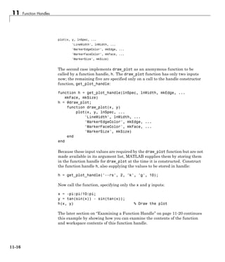
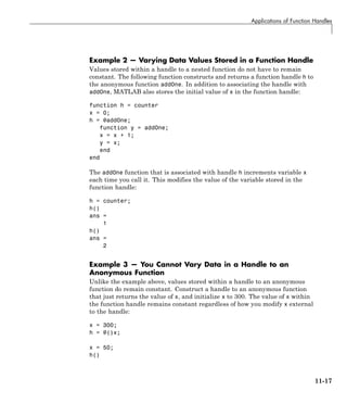
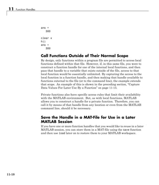
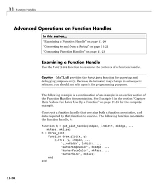
![Advanced Operations on Function Handles
Use functions to examine the contents of the returned handle:
f = functions(h)
f =
function: 'get_plot_handle/draw_plot'
type: 'nested'
file: 'D:matlabworkget_plot_handle.m'
workspace: {[1x1 struct]}
The call to functions returns a structure with four fields:
• function — Name of the function or local function to which the handle
is associated. (Function names that follow a slash character (/) are
implemented in the program code as local functions.)
• type — Type of function (e.g., simple, nested, anonymous)
• file — Filename and path to the file. (For built-in functions, this is the
string 'MATLAB built-in function')
• workspace — Variables in the function workspace at the time the handle
was constructed, along with their values
Examine the workspace variables that you saved in the function handle:
f.workspace{:}
ans =
h: @get_plot_handle/draw_plot
lnSpec: '--rs'
lnWidth: 2
mrkrEdge: 'k'
mrkrFace: 'g'
mrkrSize: 10
Converting to and from a String
Two functions, str2func and func2str enable you to convert between a
string containing a function name and a function handle that is associated
with that function name.
11-21](https://image.slidesharecdn.com/matlabprog-220902050722-ff974cdf/85/matlab_prog-pdf-395-320.jpg)
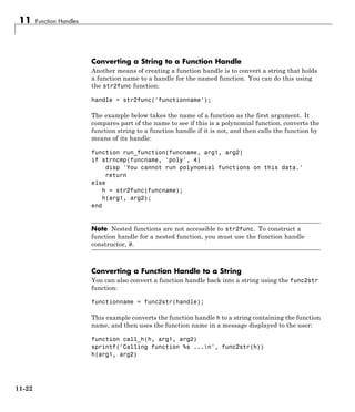
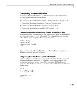
![11 Function Handles
Note In general, MATLAB may underestimate the equality of function
handles. That is, a test for equality may return false even when the functions
happen to behave the same. But in cases where MATLAB does indicate
equality, the functions are guaranteed to behave in an identical manner.
If you make a copy of an anonymous function handle, the copy and the
original are equal:
h1 = @(x)A * x.^2; h2 = h1;
isequal(h1, h2)
ans =
1
Comparing Handles to Nested Functions
MATLAB considers function handles to the same nested function to be equal
only if your code constructs these handles on the same call to the function
containing the nested functions. Given this function that constructs two
handles to the same nested function:
function [h1, h2] = test_eq(a, b, c)
h1 = @findZ;
h2 = @findZ;
function z = findZ
z = a.^3 + b.^2 + c';
end
end
function handles constructed from the same nested function and on the same
call to the parent function are considered equal:
[h1 h2] = test_eq(4, 19, -7);
isequal(h1, h2),
ans =
1
while those constructed from different calls are not considered equal:
11-24](https://image.slidesharecdn.com/matlabprog-220902050722-ff974cdf/85/matlab_prog-pdf-398-320.jpg)
![Advanced Operations on Function Handles
[q1 q2] = test_eq(3, -1, 2);
isequal(h1, q1)
ans =
0
Comparing Handles Saved to a MAT-File
If you save equivalent anonymous or nested function handles to separate
MAT-files, and then load them back into the MATLAB workspace, they are
no longer equal. This is because saving the function handle loses track of
the original circumstances under which the function handle was created.
Reloading it results in a function handle that compares as being unequal to
the original function handle.
Create two equivalent anonymous function handles:
h1 = @(x) sin(x);
h2 = h1;
isequal(h1, h2)
ans =
1
Save each to a different MAT-file:
save fname1 h1;
save fname2 h2;
Clear the MATLAB workspace, and then load the function handles back into
the workspace:
clear all
load fname1
load fname2
The function handles are no longer considered equal:
isequal(h1, h2)
ans =
11-25](https://image.slidesharecdn.com/matlabprog-220902050722-ff974cdf/85/matlab_prog-pdf-399-320.jpg)
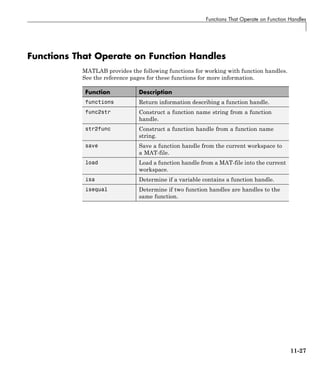

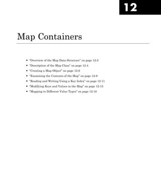
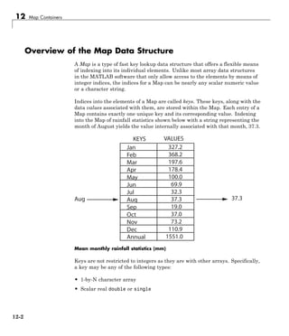
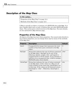
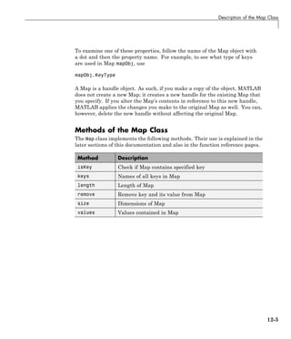
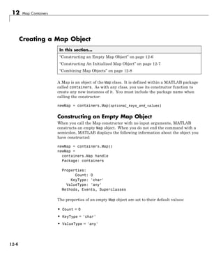
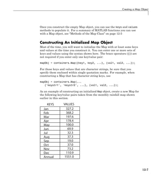
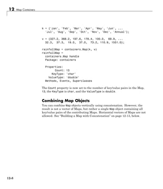
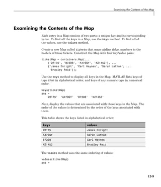
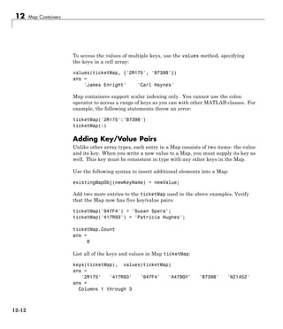
![Reading and Writing Using a Key Index
'James Enright' 'Patricia Hughes' 'Susan Spera'
Columns 4 through 6
'Sarah Latham' 'Carl Haynes' 'Bradley Reid'
Building a Map with Concatenation
You can add key/value pairs to a Map in groups using concatenation. The
concatenation of Map objects is different from other classes. Instead of
building a vector of s, MATLAB returns a single Map containing the key/value
pairs from each of the contributing Map objects.
Rules for the concatenation of Map objects are:
• Only vertical vectors of Map objects are allowed. You cannot create an
m-by-n array or a horizontal vector of s. For this reason, vertcat is
supported for Map objects, but not horzcat.
• All keys in each map being concatenated must be of the same class.
• You can combine Maps with different numbers of key/value pairs. The
result is a single Map object containing key/value pairs from each of the
contributing maps:
tMap1 = containers.Map({'2R175', 'B7398', 'A479GY'}, ...
{'James Enright', 'Carl Haynes', 'Sarah Latham'});
tMap2 = containers.Map({'417R93', 'NZ1452', '947F4'}, ...
{'Patricia Hughes', 'Bradley Reid', 'Susan Spera'});
% Concatenate the two maps:
ticketMap = [tMap1; tMap2];
The result of this concatenation is the same 6-element map that was
constructed in the previous section:
ticketMap.Count
ans =
6
keys(ticketMap), values(ticketMap)
ans =
'2R175' '417R93' '947F4' 'A479GY' 'B7398' 'NZ1452'
12-13](https://image.slidesharecdn.com/matlabprog-220902050722-ff974cdf/85/matlab_prog-pdf-415-320.jpg)
![12 Map Containers
ans =
Columns 1 through 3
'James Enright' 'Patricia Hughes' 'Susan Spera'
Columns 4 through 6
'Sarah Latham' 'Carl Haynes' 'Bradley Reid'
• Concatenation does not include duplicate keys or their values in the
resulting Map object.
In the following example, both objects m1 and m2 use a key of 8. In Map m1,
8 is a key to value C; in m2, it is a key to value X:
m1 = containers.Map({1, 5, 8}, {'A', 'B', 'C'});
m2 = containers.Map({8, 9, 6}, {'X', 'Y', 'Z'});
Combine m1 and m2 to form a new Map object, m:
m = [m1; m2];
The resulting Map object m has only five key/value pairs. The value C was
dropped from the concatenation because its key was not unique:
keys(m), values(m)
ans =
[1] [5] [6] [8] [9]
ans =
'A' 'B' 'Z' 'X' 'Y'
12-14](https://image.slidesharecdn.com/matlabprog-220902050722-ff974cdf/85/matlab_prog-pdf-416-320.jpg)
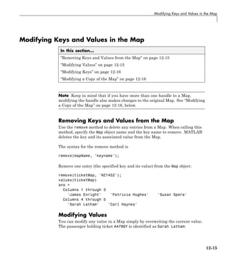
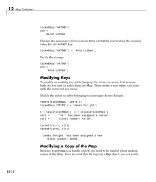
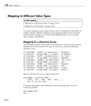
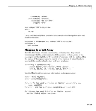

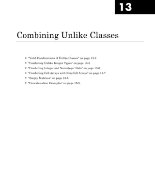
![Combining Unlike Integer Types
Combining Unlike Integer Types
In this section...
“Overview” on page 13-3
“Example of Combining Unlike Integer Sizes” on page 13-4
“Example of Combining Signed with Unsigned” on page 13-4
Overview
If you combine different integer types in a matrix (e.g., signed with unsigned,
or 8-bit integers with 16-bit integers), MATLAB returns a matrix in which all
elements are of one common type. MATLAB sets all elements of the resulting
matrix to the data type of the left-most element in the input matrix. For
example, the result of the following concatenation is a vector of three 16-bit
signed integers:
A = [int16(450) uint8(250) int32(1000000)]
MATLAB also displays a warning to inform you that the result may not be
what you had expected:
A = [int16(450) uint8(250) int32(1000000)];
Warning: Concatenation with dominant (left-most) integer class
may overflow other operands on conversion to return class.
You can disable this warning by entering the following two commands directly
after the operation that caused the warning. The first command retrieves
the message identifier associated with the most recent warning issued by
MATLAB. The second command uses this identifier to disable any further
warnings of that type from being issued:
[msg, intcat_msgid] = lastwarn;
warning('off', intcat_msgid);
To re-enable the warning so that it will now be displayed, use
warning('on', intcat_msgid);
13-3](https://image.slidesharecdn.com/matlabprog-220902050722-ff974cdf/85/matlab_prog-pdf-425-320.jpg)
![13 Combining Unlike Classes
You can use these commands to disable or enable the display of any MATLAB
warning.
Example of Combining Unlike Integer Sizes
After disabling the integer concatenation warnings as shown above,
concatenate the following two numbers once, and then switch their order. The
return value depends on the order in which the integers are concatenated.
The left-most type determines the data type for all elements in the vector:
A = [int16(5000) int8(50)]
A =
5000 50
B = [int8(50) int16(5000)]
B =
50 127
The first operation returns a vector of 16-bit integers. The second returns a
vector of 8-bit integers. The element int16(5000) is set to 127, the maximum
value for an 8-bit signed integer.
The same rules apply to vertical concatenation:
C = [int8(50); int16(5000)]
C =
50
127
Note You can find the maximum or minimum values for any MATLAB
integer type using the intmax and intmin functions. For floating-point types,
use realmax and realmin.
Example of Combining Signed with Unsigned
Now do the same exercise with signed and unsigned integers. Again, the
left-most element determines the data type for all elements in the resulting
matrix:
13-4](https://image.slidesharecdn.com/matlabprog-220902050722-ff974cdf/85/matlab_prog-pdf-426-320.jpg)
![Combining Unlike Integer Types
A = [int8(-100) uint8(100)]
A =
-100 100
B = [uint8(100) int8(-100)]
B =
100 0
The element int8(-100) is set to zero because it is no longer signed.
MATLAB evaluates each element prior to concatenating them into a combined
array. In other words, the following statement evaluates to an 8-bit signed
integer (equal to 50) and an 8-bit unsigned integer (unsigned -50 is set to
zero) before the two elements are combined. Following the concatenation, the
second element retains its zero value but takes on the unsigned int8 type:
A = [int8(50), uint8(-50)]
A =
50 0
13-5](https://image.slidesharecdn.com/matlabprog-220902050722-ff974cdf/85/matlab_prog-pdf-427-320.jpg)
![13 Combining Unlike Classes
Combining Integer and Noninteger Data
If you combine integers with double, single, or logical classes, all elements
of the resulting matrix are given the data type of the left-most integer. For
example, all elements of the following vector are set to int32:
A = [true pi int32(1000000) single(17.32) uint8(250)]
13-6](https://image.slidesharecdn.com/matlabprog-220902050722-ff974cdf/85/matlab_prog-pdf-428-320.jpg)
![Combining Cell Arrays with Non-Cell Arrays
Combining Cell Arrays with Non-Cell Arrays
Combining a number of arrays in which one or more is a cell array returns a
new cell array. Each of the original arrays occupies a cell in the new array:
A = [100, {uint8(200), 300}, 'MATLAB'];
whos A
Name Size Bytes Class Attributes
A 1x4 477 cell
Each element of the combined array maintains its original class:
fprintf('Classes: %s %s %s %sn',...
class(A{1}),class(A{2}),class(A{3}),class(A{4}))
Classes: double uint8 double char
13-7](https://image.slidesharecdn.com/matlabprog-220902050722-ff974cdf/85/matlab_prog-pdf-429-320.jpg)
![13 Combining Unlike Classes
Empty Matrices
If you construct a matrix using empty matrix elements, the empty matrices
are ignored in the resulting matrix:
A = [5.36; 7.01; []; 9.44]
A =
5.3600
7.0100
9.4400
13-8](https://image.slidesharecdn.com/matlabprog-220902050722-ff974cdf/85/matlab_prog-pdf-430-320.jpg)
![Concatenation Examples
Concatenation Examples
In this section...
“Combining Single and Double Types” on page 13-9
“Combining Integer and Double Types” on page 13-9
“Combining Character and Double Types” on page 13-10
“Combining Logical and Double Types” on page 13-10
Combining Single and Double Types
Combining single values with double values yields a single matrix. Note
that 5.73*10^300 is too big to be stored as a single, thus the conversion from
double to single sets it to infinity. (The class function used in this example
returns the data type for the input value).
x = [single(4.5) single(-2.8) pi 5.73*10^300]
x =
4.5000 -2.8000 3.1416 Inf
class(x) % Display the data type of x
ans =
single
Combining Integer and Double Types
Combining integer values with double values yields an integer matrix. Note
that the fractional part of pi is rounded to the nearest integer. (The int8
function used in this example converts its numeric argument to an 8-bit
integer).
x = [int8(21) int8(-22) int8(23) pi 45/6]
x =
21 -22 23 3 8
class(x)
ans =
int8
13-9](https://image.slidesharecdn.com/matlabprog-220902050722-ff974cdf/85/matlab_prog-pdf-431-320.jpg)
![13 Combining Unlike Classes
Combining Character and Double Types
Combining character values with double values yields a character matrix.
MATLAB converts the double elements in this example to their character
equivalents:
x = ['A' 'B' 'C' 68 69 70]
x =
ABCDEF
class(x)
ans =
char
Combining Logical and Double Types
Combining logical values with double values yields a double matrix.
MATLAB converts the logical true and false elements in this example to
double:
x = [true false false pi sqrt(7)]
x =
1.0000 0 0 3.1416 2.6458
class(x)
ans =
double
13-10](https://image.slidesharecdn.com/matlabprog-220902050722-ff974cdf/85/matlab_prog-pdf-432-320.jpg)
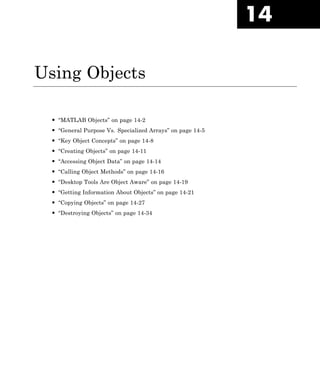
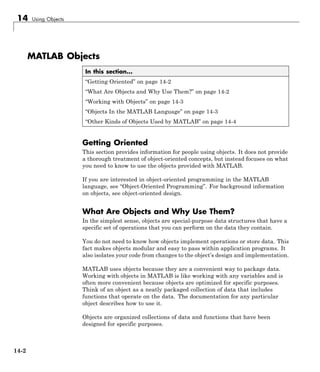
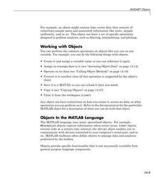
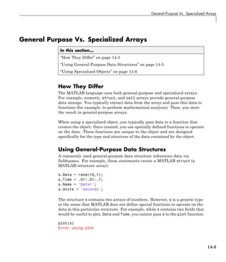
![14 Using Objects
Not enough input arguments.
While s has enough information to create a plot of Data versus Time, plot
cannot access this data because structures like s can contain any values in
its fields and the fields can have any name. Just because one field is named
Data does not force you to assign data to that field.
To plot the data in s, you have to extract the data from the fields, pass them
as numeric arrays in the desired order to the plot function, add a title,
labels, and so on:
plot(s.Time,s.Data)
title(['Time Series Plot: ' s.Name])
xlabel(['Time (' s.Units ')'])
ylabel(s.Name)
You could create a function to perform these steps for you. Other programs
using the structure s would need to create their own functions or access the
one you created.
Using Specialized Objects
Compare the array s above to an object that you have designed specifically
to contain and manipulate time series data. For example, the following
statement creates a MATLAB® timeseries object. It is initialized to store
the same data as the structure s above:
tsobj = timeseries(rand(10,1),.01:.01:.1,'Name','Data1');
The function that creates the object tsobj, accepts sample data, sample
times, a property name/property value pair (Name/Data1), and uses a default
value of Units (which is seconds).
The designer of this object created a special version of the plot function that
works directly with this object. For example:
plot(tsobj)
14-6](https://image.slidesharecdn.com/matlabprog-220902050722-ff974cdf/85/matlab_prog-pdf-438-320.jpg)
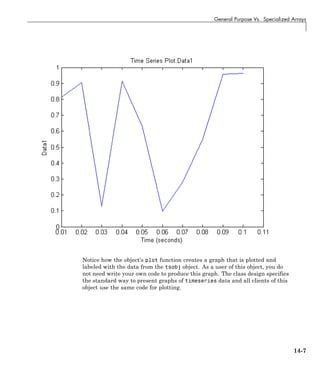
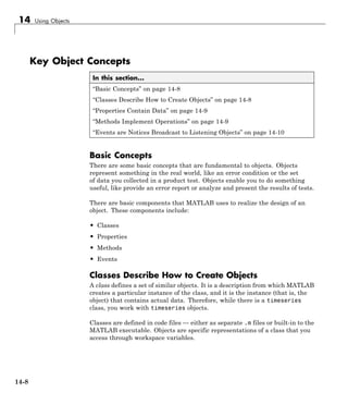
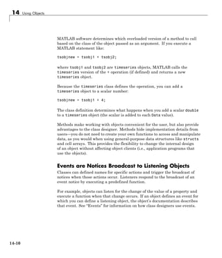
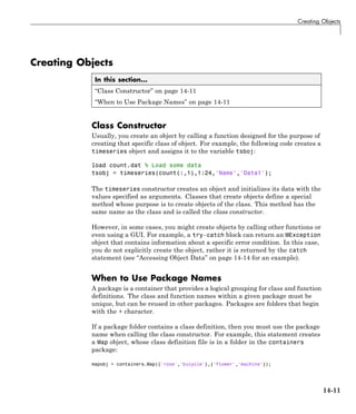
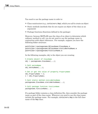
![14 Using Objects
Accessing Object Data
In this section...
“Listing Public Properties” on page 14-14
“Getting Property Values” on page 14-14
“Setting Property Values” on page 14-15
Listing Public Properties
Note Always use the correct case when referring to properties by name.
Display the names of all public object properties using the properties
function with the object’s class name or with an actual object. For example:
>> properties('MException')
Properties for class MException:
identifier
message
cause
stack
Getting Property Values
After creating an object, you can access the values of its properties:
try
a = rand(4);
a(17) = 7;
catch me % catch creates an MException object named me
disp(['Current error identifier: ' me.identifier])
end
Current error identifier: MATLAB:indexed_matrix_cannot_be_resized
Access the data in properties using dot notation:
object.PropertyName
14-14](https://image.slidesharecdn.com/matlabprog-220902050722-ff974cdf/85/matlab_prog-pdf-446-320.jpg)
![Accessing Object Data
For example, you can access the message property of the MException object,
me, with this syntax:
me.message
ans =
In an assignment A(I) = B, a matrix A cannot be resized.
See “Capture Information About Exceptions” on page 23-5 for more
information on using MException objects.
Setting Property Values
Objects often restrict what values you can assign to them. For example, the
following timeseries object has 10 data values, each corresponding to a
sample time:
tsobj = timeseries(rand(10,1),1:10,'Name','Random Sample');
Now suppose you attempt to set the Data property to a three-element vector:
tsobj.Data = [1 2 3];
Error using timeseries.utreshape (line 864)
Size of the data array is incompatible with the time vector.
...
The timeseries class design ensures that the number of data samples
matches the number of time samples. This illustrates one of the advantages a
specialized object has over a general purpose-data structure like a MATLAB
struct.
14-15](https://image.slidesharecdn.com/matlabprog-220902050722-ff974cdf/85/matlab_prog-pdf-447-320.jpg)
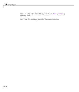
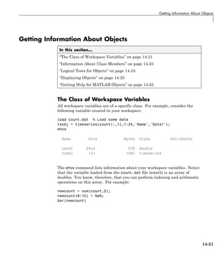
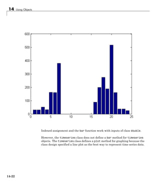
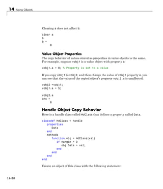
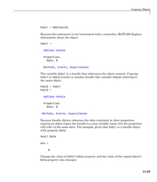
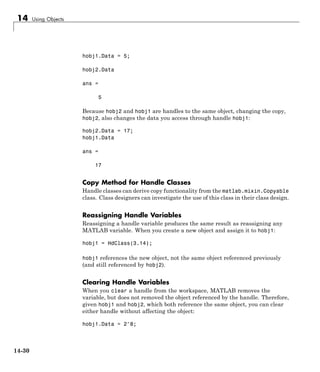

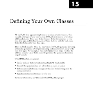

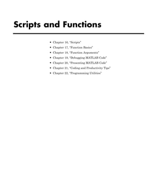

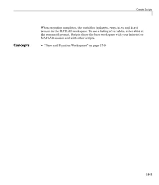
![16 Scripts
Add Comments to Programs
This topic explains how and why to add comments to your program files.
When you write code, it is a good practice to add comments that describe
the code. Comments allow others to understand your code, and can refresh
your memory when you return to it later. Add comments to MATLAB code
using the percent (%) symbol.
Comment lines can appear anywhere in a program file, and you can append
comments to the end of a line of code. For example,
% Add up all the vector elements.
y = sum(x) % Use the sum function.
Comments are also useful for program development and testing—comment
out any code that does not need to run. To comment out multiple lines of code,
you can use the block comment operators, %{ and %}:
a = magic(3);
%{
sum(a)
diag(a)
sum(diag(a))
%}
sum(diag(fliplr(a)))
The %{ and %} operators must appear alone on the lines that immediately
precede and follow the block of help text. Do not include any other text on
these lines.
To comment out part of a statement that spans multiple lines, use an ellipses
(...) instead of a percent sign. For example,
header = ['Last Name, ', ...
'First Name, ', ...
... 'Middle Initial, ', ...
'Title']
16-4](https://image.slidesharecdn.com/matlabprog-220902050722-ff974cdf/85/matlab_prog-pdf-476-320.jpg)
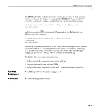
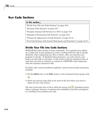
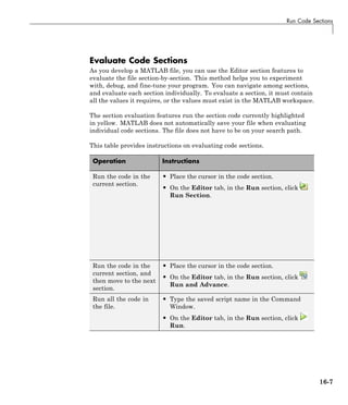
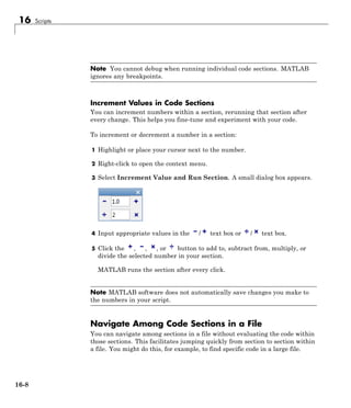
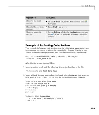
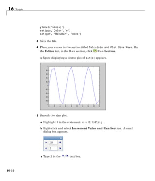
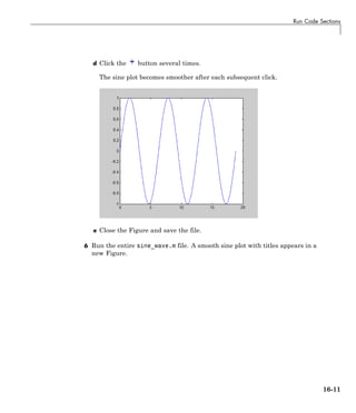
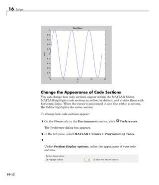
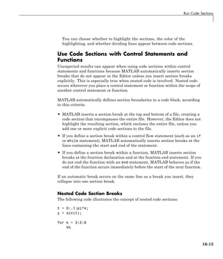
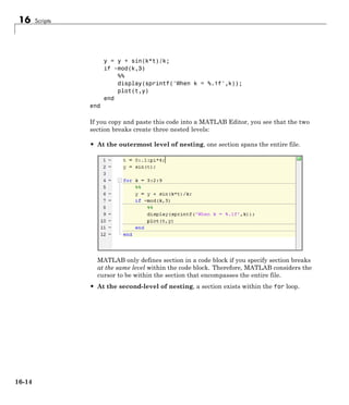
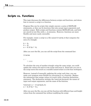
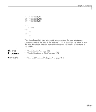

![17 Function Basics
Create Functions in Files
This example shows how to create a function in a program file.
Write a Function
Open a file in a text editor. Within the file, declare the function and add
program statements:
function f = fact(n)
f = prod(1:n);
Function fact accepts a single input argument n, and returns the factorial
of n in output argument f.
The definition statement is the first executable line of any function. Function
definitions are not valid at the command line or within a script. Each function
definition includes these elements.
function keyword
(required)
Use lowercase characters for the keyword.
Output arguments
(optional)
If your function returns more than one output,
enclose the output names in square brackets, such as
function [one,two,three] = myfunction(x)
If there is no output, either omit it,
function myfunction(x)
or use empty square brackets:
function [] = myfunction(x)
17-2](https://image.slidesharecdn.com/matlabprog-220902050722-ff974cdf/85/matlab_prog-pdf-492-320.jpg)
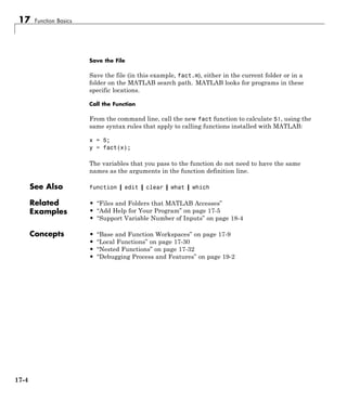
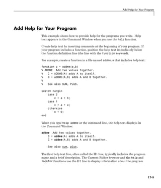
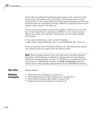
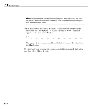
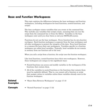
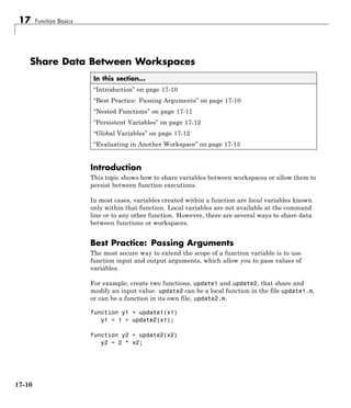
![Share Data Between Workspaces
Call the update1 function from the command line and assign to variable Y in
the base workspace:
X = [1,2,3];
Y = update1(X)
Y =
3 5 7
Nested Functions
A nested function has access to the workspaces of all functions in which it is
nested. So, for example, a nested function can use a variable (in this case, x)
that is defined in its parent function:
function primaryFx
x = 1;
nestedFx;
function nestedFx
x = x + 1;
end
end
When parent functions do not use a given variable, the variable remains
local to the nested function. For example, in this version of primaryFx, the
two nested functions have their own versions of x that cannot interact with
each other.
function primaryFx
nestedFx1;
nestedFx2;
function nestedFx1
x = 1;
end
function nestedFx2
x = 2;
end
end
17-11](https://image.slidesharecdn.com/matlabprog-220902050722-ff974cdf/85/matlab_prog-pdf-501-320.jpg)
![17 Function Basics
For more information, see “Nested Functions” on page 17-32.
Persistent Variables
When you declare a variable within a function as persistent, the variable
retains its value from one function call to the next. Other local variables
retain their value only during the current execution of a function. Persistent
variables are equivalent to static variables in other programming languages.
Declare variables using the persistent keyword before you use them.
MATLAB initializes persistent variables to an empty matrix, [].
For example, define a function in a file named findSum.m that initializes a
sum to 0, and then adds to the value on each iteration.
function findSum(inputvalue)
persistent SUM_X
if isempty(SUM_X)
SUM_X = 0;
end
SUM_X = SUM_X + inputvalue;
When you call the function, the value of SUM_X persists between subsequent
executions.
These operations clear the persistent variables for a function:
• clear all
• clear functionname
• Editing the function file
To prevent clearing persistent variables, lock the function file using mlock.
Global Variables
Global variables are variables that you can access from functions or from
the command line. They have their own workspace, which is separate from
the base and function workspaces.
17-12](https://image.slidesharecdn.com/matlabprog-220902050722-ff974cdf/85/matlab_prog-pdf-502-320.jpg)
![17 Function Basics
Like global variables, these functions carry risks of overwriting existing data.
Use them sparingly.
evalin and assignin are sometimes useful for callback functions in graphical
user interfaces to evaluate against the base workspace. For example, create a
list box of variable names from the base workspace:
function listBox
figure;
lb = uicontrol('Style','listbox','Position',[10 10 100 100],...
'Callback',@update_listBox);
update_listBox(lb)
function update_listBox(src,~)
vars = evalin('base','who');
set(src,'String',vars)
For other programming applications, consider argument passing and the
techniques described in “Alternatives to the eval Function” on page 2-69.
Concepts • “Base and Function Workspaces” on page 17-9
17-14](https://image.slidesharecdn.com/matlabprog-220902050722-ff974cdf/85/matlab_prog-pdf-504-320.jpg)
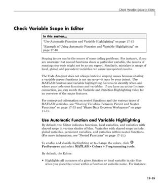
![17 Function Basics
• Displays a variable with shared scope in teal blue, regardless of the cursor
location. For instance:
Example of Using Automatic Function and Variable
Highlighting
Consider the code for a function rowsum:
function rowTotals = rowsum
% Add the values in each row and
% store them in a new array
x = ones(2,10);
[n, m] = size(x);
rowTotals = zeros(1,n);
for i = 1:n
rowTotals(i) = addToSum;
end
function colsum = addToSum
colsum = 0;
thisrow = x(i,:);
for i = 1:m
colsum = colsum + thisrow(i);
end
end
end
When you run this code, instead of returning the sum of the values in each
row and displaying:
ans =
10 10
MATLAB displays:
17-16](https://image.slidesharecdn.com/matlabprog-220902050722-ff974cdf/85/matlab_prog-pdf-506-320.jpg)
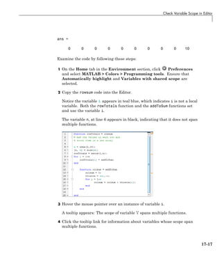
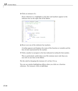
![17 Function Basics
Nested functions are completely contained within another function. The
primary difference between nested functions and local functions is that nested
functions can use variables defined in parent functions without explicitly
passing those variables as arguments.
Nested functions are useful when subroutines share data, such as GUI
applications that pass data between components. For example, create a
function that allows you to set a value between 0 and 1 using either a slider
or an editable text box. If you use nested functions for the callbacks, the
slider and text box can share the value and each other’s handles without
explicitly passing them:
function myslider
value = 0;
f = figure;
s = uicontrol(f,'Style','slider','Callback',@slider);
e = uicontrol(f,'Style','edit','Callback',@edittext,...
'Position',[100,20,100,20]);
function slider(obj,~)
value = get(obj,'Value');
set(e,'String',num2str(value));
end
function edittext(obj,~)
value = str2double(get(obj,'String'));
set(s,'Value',value);
end
end
Private Functions in a Subfolder
Like local or nested functions, private functions are accessible only to
functions in a specific location. However, private functions are not in the
same file as the functions that can call them. Instead, they are in a subfolder
named private. Private functions are available only to functions in the folder
immediately above the private folder. Use private functions to separate code
into different files, or to share code between multiple, related functions.
17-20](https://image.slidesharecdn.com/matlabprog-220902050722-ff974cdf/85/matlab_prog-pdf-510-320.jpg)
![Types of Functions
Anonymous Functions Without a File
Anonymous functions allow you to define a function without creating a
program file, as long as the function consists of a single statement. A common
application of anonymous functions is to define a mathematical expression,
and then evaluate that expression over a range of values using a MATLAB®
function function, i.e., a function that accepts a function handle as an input.
For example, this statement creates a function handle named s for an
anonymous function:
s = @(x) sin(1./x);
This function has a single input, x . The @ operator creates the function
handle.
You can use the function handle to evaluate the function for particular values,
such as
y = s(pi)
y =
0.3130
Or, you can pass the function handle to a function that evaluates over a range
of values, such as fplot:
range = [0.01,0.1];
fplot(s,range)
17-21](https://image.slidesharecdn.com/matlabprog-220902050722-ff974cdf/85/matlab_prog-pdf-511-320.jpg)
![Anonymous Functions
y = 10;
z = myfunction(x,y)
z =
111
However, you do not explicitly define output arguments when you create
an anonymous function. If the expression in the function returns multiple
outputs, then you can request them when you call the function. Enclose
multiple output variables in square brackets.
For example, the ndgrid function can return as many outputs as the number
of input vectors. This anonymous function that calls ndgrid can also return
multiple outputs:
c = 10;
mygrid = @(x,y) ndgrid((-x:x/c:x),(-y:y/c:y));
[x,y] = mygrid(pi,2*pi);
You can use the output from mygrid to create a mesh or surface plot:
z = sin(x) + cos(y);
mesh(x,y,z)
17-27](https://image.slidesharecdn.com/matlabprog-220902050722-ff974cdf/85/matlab_prog-pdf-517-320.jpg)
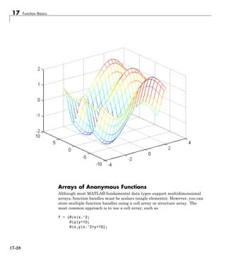
![17 Function Basics
Local Functions
This topic explains the term local function, and shows how to create and
use local functions.
MATLAB program files can contain code for more than one function. The first
function in the file (the main function) is visible to functions in other files, or
you can call it from the command line. Additional functions within the file
are called local functions. Local functions are only visible to other functions
in the same file. They are equivalent to subroutines in other programming
languages, and are sometimes called subfunctions.
Local functions can occur in any order, as long as the main function appears
first. Each function begins with its own function definition line.
For example, create a program file named mystats.m that contains a main
function, mystats, and two local functions, mymean and mymedian.
function [avg, med] = mystats(x)
n = length(x);
avg = mymean(x,n);
med = mymedian(x,n);
end
function a = mymean(v,n)
% MYMEAN Example of a local function.
a = sum(v)/n;
end
function m = mymedian(v,n)
% MYMEDIAN Another example of a local function.
w = sort(v);
if rem(n,2) == 1
m = w((n + 1)/2);
else
m = (w(n/2) + w(n/2 + 1))/2;
end
end
17-30](https://image.slidesharecdn.com/matlabprog-220902050722-ff974cdf/85/matlab_prog-pdf-520-320.jpg)
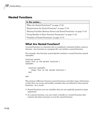
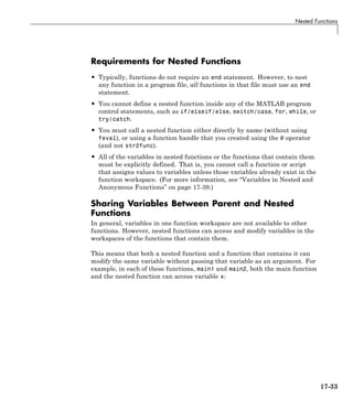
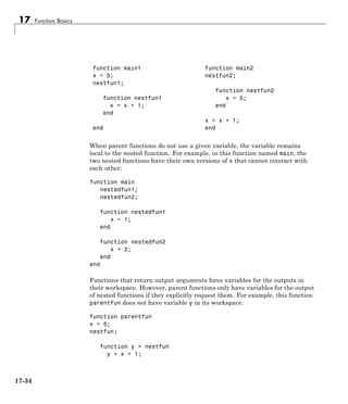
![17 Function Basics
end
The makeParabola function returns a handle to the parabola function that
includes values for coefficients a, b, and c.
At the command line, call the makeParabola function with coefficient values
of 1.3, .2, and 30. Use the returned function handle p to evaluate the
polynomial at a particular point:
p = makeParabola(1.3,.2,30);
X = 25;
Y = p(X)
Y =
847.5000
Many MATLAB functions accept function handle inputs to evaluate functions
over a range of values. For example, plot the parabolic equation from -25 to
+25:
fplot(p,[-25,25])
17-36](https://image.slidesharecdn.com/matlabprog-220902050722-ff974cdf/85/matlab_prog-pdf-526-320.jpg)
![Nested Functions
You can create multiple handles to the parabola function that each use
different polynomial coefficients:
firstp = makeParabola(0.8,1.6,32);
secondp = makeParabola(3,4,50);
range = [-25,25];
figure
hold on
fplot(firstp,range)
fplot(secondp,range,'r:')
hold off
Visibility of Nested Functions
Every function has a certain scope, that is, a set of other functions to which it
is visible. A nested function is available:
• From the level immediately above it. (In the following code, function A can
call B or D, but not C or E.)
17-37](https://image.slidesharecdn.com/matlabprog-220902050722-ff974cdf/85/matlab_prog-pdf-527-320.jpg)
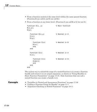
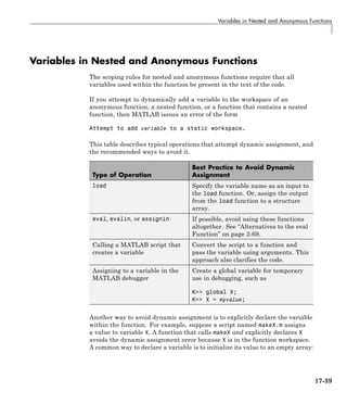
![17 Function Basics
function noerror
X = [];
nestedfx
function nestedfx
makeX
end
end
Concepts • “Base and Function Workspaces” on page 17-9
17-40](https://image.slidesharecdn.com/matlabprog-220902050722-ff974cdf/85/matlab_prog-pdf-530-320.jpg)
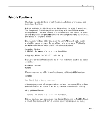
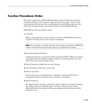
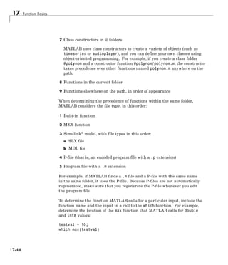
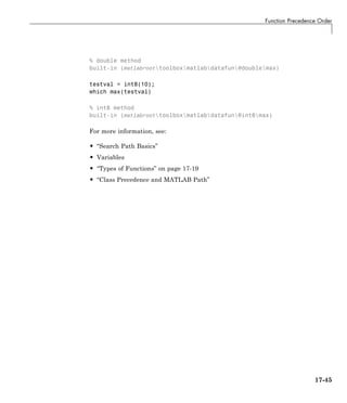

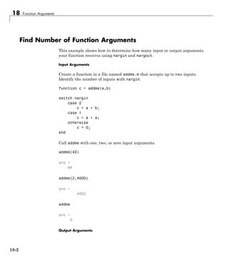
![Find Number of Function Arguments
Create a new function in a file named addme2.m that can return one or two
outputs (a result and its absolute value). Identify the number of requested
outputs with nargout.
function [result,absResult] = addme2(a,b)
switch nargin
case 2
result = a + b;
case 1
result = a + a;
otherwise
result = 0;
end
if nargout > 1
absResult = abs(result);
end
Call addme2 with one or two output arguments.
value = addme2(11,-22)
value =
-11
[value,absValue] = addme2(11,-22)
value =
-11
absValue =
11
Functions return outputs in the order they are declared in the function
definition.
See Also nargin | narginchk | nargout | nargoutchk
18-3](https://image.slidesharecdn.com/matlabprog-220902050722-ff974cdf/85/matlab_prog-pdf-539-320.jpg)
![18 Function Arguments
Support Variable Number of Inputs
This example shows how to define a function that accepts a variable number
of input arguments using varargin. The varargin argument is a cell array
that contains the function inputs, where each input is in its own cell.
Create a function in a file named plotWithTitle.m that accepts a variable
number of paired (x,y) inputs for the plot function and an optional title. If
the function receives an odd number of inputs, it assumes that the last input
is a title.
function plotWithTitle(varargin)
if rem(nargin,2) ~= 0
myTitle = varargin{nargin};
numPlotInputs = nargin - 1;
else
myTitle = 'Default Title';
numPlotInputs = nargin;
end
plot(varargin{1:numPlotInputs})
title(myTitle)
Because varargin is a cell array, you access the contents of each cell
using curly braces, {}. The syntax varargin{1:numPlotInputs} creates a
comma-separated list of inputs to the plot function.
Call plotWithTitle with two sets of (x,y) inputs and a title.
x = [1:.1:10]; y1 = sin(x); y2 = cos(x);
plotWithTitle(x,y1,x,y2,'Sine and Cosine')
You can use varargin alone in an input argument list, or at the end of the
list of inputs, such as
function myfunction(a,b,varargin)
In this case, varargin{1} corresponds to the third input passed to the
function, and nargin returns length(varargin) + 2.
See Also nargin | varargin
18-4](https://image.slidesharecdn.com/matlabprog-220902050722-ff974cdf/85/matlab_prog-pdf-540-320.jpg)
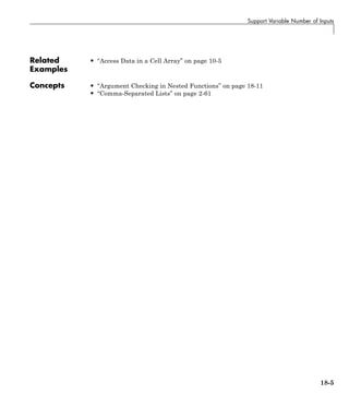
![18 Function Arguments
Support Variable Number of Outputs
This example shows how to define a function that returns a variable number
of output arguments using varargout. Output varargout is a cell array that
contains the function outputs, where each output is in its own cell.
Create a function in a file named magicfill.m that assigns a magic square to
each requested output.
function varargout = magicfill
nOutputs = nargout;
varargout = cell(1,nOutputs);
for k = 1:nOutputs;
varargout{k} = magic(k);
end
Indexing with curly braces {} updates the contents of a cell.
Call magicfill and request three outputs.
[first,second,third] = magicfill
first =
1
second =
1 3
4 2
third =
8 1 6
3 5 7
4 9 2
MATLAB assigns values to the outputs according to their order in the
varargout array. For example, first == varargout{1}.
You can use varargout alone in an output argument list, or at the end of
the list of outputs, such as
18-6](https://image.slidesharecdn.com/matlabprog-220902050722-ff974cdf/85/matlab_prog-pdf-542-320.jpg)
![Support Variable Number of Outputs
function [x,y,varargout] = myfunction(a,b)
In this case, varargout{1} corresponds to the third output that the function
returns, and nargout returns length(varargout) + 2.
See Also nargout | varargout
Related
Examples
• “Access Data in a Cell Array” on page 10-5
Concepts • “Argument Checking in Nested Functions” on page 18-11
18-7](https://image.slidesharecdn.com/matlabprog-220902050722-ff974cdf/85/matlab_prog-pdf-543-320.jpg)
![18 Function Arguments
Validate Number of Function Arguments
This example shows how to check whether your custom function receives
a valid number of input or output arguments. MATLAB performs some
argument checks automatically. For other cases, you can use narginchk or
nargoutchk.
Automatic Argument Checks
MATLAB checks whether your function receives more arguments than
expected when it can determine the number from the function definition. For
example, this function accepts up to two outputs and three inputs:
function [x,y] = myFunction(a,b,c)
If you pass too many inputs to myFunction, MATLAB issues an error. You do
not need to call narginchk to check for this case.
[X,Y] = myFunction(1,2,3,4)
Error using myFunction
Too many input arguments.
Use the narginchk and nargoutchk functions to verify that your function
receives:
• A minimum number of required arguments.
• No more than a maximum number of arguments, when your function uses
varargin or varargout.
Input Checks with narginchk
Define a function in a file named testValues.m that requires at least two
inputs. The first input is a threshold value to compare against the other
inputs.
function testValues(threshold,varargin)
minInputs = 2;
maxInputs = Inf;
narginchk(minInputs,maxInputs)
18-8](https://image.slidesharecdn.com/matlabprog-220902050722-ff974cdf/85/matlab_prog-pdf-544-320.jpg)
![Validate Number of Function Arguments
for k = 1:(nargin-1)
if (varargin{k} > threshold)
fprintf('Test value %d exceeds %dn',k,threshold);
end
end
Call testValues with too few inputs.
testValues(10)
Error using testValues (line 4)
Not enough input arguments.
Call testValues with enough inputs.
testValues(10,1,11,111)
Test value 2 exceeds 10
Test value 3 exceeds 10
Output Checks with nargoutchk
Define a function in a file named mysize.m that returns the dimensions of
the input array in a vector (from the size function), and optionally returns
scalar values corresponding to the sizes of each dimension. Use nargoutchk
to verify that the number of requested individual sizes does not exceed the
number of available dimensions.
function [sizeVector,varargout] = mysize(x)
minOutputs = 0;
maxOutputs = ndims(x) + 1;
nargoutchk(minOutputs,maxOutputs)
sizeVector = size(x);
varargout = cell(1,nargout-1);
for k = 1:length(varargout)
varargout{k} = sizeVector(k);
end
Call mysize with a valid number of outputs.
18-9](https://image.slidesharecdn.com/matlabprog-220902050722-ff974cdf/85/matlab_prog-pdf-545-320.jpg)
![18 Function Arguments
A = rand(3,4,2);
[fullsize,nrows,ncols,npages] = mysize(A)
fullsize =
3 4 2
nrows =
3
ncols =
4
npages =
2
Call mysize with too many outputs.
A = 1;
[fullsize,nrows,ncols,npages] = mysize(A)
Error using mysize (line 4)
Too many output arguments.
See Also narginchk | nargoutchk
Related
Examples
• “Support Variable Number of Inputs” on page 18-4
• “Support Variable Number of Outputs” on page 18-6
18-10](https://image.slidesharecdn.com/matlabprog-220902050722-ff974cdf/85/matlab_prog-pdf-546-320.jpg)
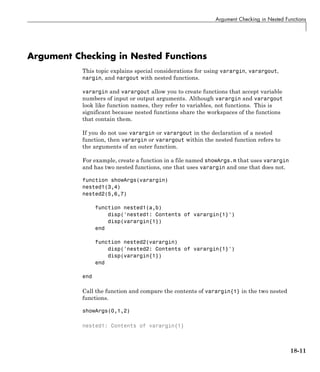
![18 Function Arguments
0
nested2: Contents of varargin{1}
5
On the other hand, nargin and nargout are functions. Within any function,
including nested functions, calls to nargin or nargout return the number of
arguments for that function. If a nested function requires the value of nargin
or nargout from an outer function, pass the value to the nested function.
For example, create a function in a file named showNumArgs.m that passes
the number of input arguments from the primary (parent) function to a
nested function.
function showNumArgs(varargin)
disp(['Number of inputs to showNumArgs: ',int2str(nargin)]);
nestedFx(nargin,2,3,4)
function nestedFx(n,varargin)
disp(['Number of inputs to nestedFx: ',int2str(nargin)]);
disp(['Number of inputs to its parent: ',int2str(n)]);
end
end
Call showNumArgs and compare the output of nargin in the parent and nested
functions.
showNumArgs(0,1)
Number of inputs to showNumArgs: 2
Number of inputs to nestedFx: 4
Number of inputs to its parent: 2
See Also nargin | nargout | varargin | varargout
18-12](https://image.slidesharecdn.com/matlabprog-220902050722-ff974cdf/85/matlab_prog-pdf-548-320.jpg)
![18 Function Arguments
Check Function Inputs with validateattributes
This example shows how to verify that the inputs to your function conform to
a set of requirements using the validateattributes function.
validateattributes requires that you pass the variable to check and the
supported data types for that variable. Optionally, pass a set of attributes
that describe the valid dimensions or values.
Check Data Type and Other Attributes
Define a function in a file named checkme.m that accepts up to three inputs:
a, b, and c. Check whether:
• a is a two-dimensional array of positive double-precision values.
• b contains 100 numeric values in an array with 10 columns.
• c is a nonempty character string or cell array.
function checkme(a,b,c)
validateattributes(a,{'double'},{'positive','2d'})
validateattributes(b,{'numeric'},{'numel',100,'ncols',10})
validateattributes(c,{'char','cell'},{'nonempty'})
disp('All inputs are ok.')
The curly braces {} indicate that the set of data types and the set of additional
attributes are in cell arrays. Cell arrays allow you to store combinations of
text and numeric data, or text strings of different lengths, in a single variable.
Call checkme with valid inputs.
checkme(pi,rand(5,10,2),'text')
All inputs are ok.
The scalar value pi is two-dimensional because size(pi) = [1,1].
18-14](https://image.slidesharecdn.com/matlabprog-220902050722-ff974cdf/85/matlab_prog-pdf-550-320.jpg)
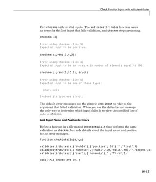
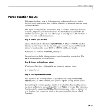
![Parse Function Inputs
By default, the Input Parser makes assumptions about case sensitivity,
function names, structure array inputs, and whether to allow additional
parameter names and values that are not in the scheme. Properties allow you
to explicitly define the behavior. Set properties using dot notation, similar to
assigning values to a structure array.
Allow printPhoto to accept additional parameter value inputs that do not
match the input scheme by setting the KeepUnmatched property of the Input
Parser.
p.KeepUnmatched = true;
If KeepUnmatched is false (default), the Input Parser issues an error when
inputs do not match the scheme.
Step 5. Parse the inputs.
Within your function, call the parse method. Pass the values of all of the
function inputs.
parse(p,filename,varargin{:});
Step 6. Use the inputs in your function.
Access parsed inputs using these properties of the inputParser object:
• Results — Structure array with names and values of all inputs in the
scheme.
• Unmatched — Structure array with parameter names and values that are
passed to the function, but are not in the scheme (when KeepUnmatched
is true).
• UsingDefaults — Cell array with names of optional inputs that are
assigned their default values because they are not passed to the function.
Within the printPhoto function, display the values for some of the inputs:
disp(['File name: ',p.Results.filename])
disp(['Finish: ', p.Results.finish])
if ~isempty(fieldnames(p.Unmatched))
18-19](https://image.slidesharecdn.com/matlabprog-220902050722-ff974cdf/85/matlab_prog-pdf-555-320.jpg)
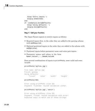
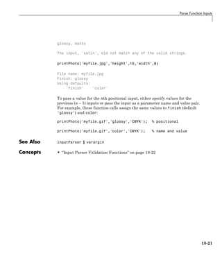
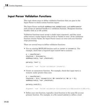

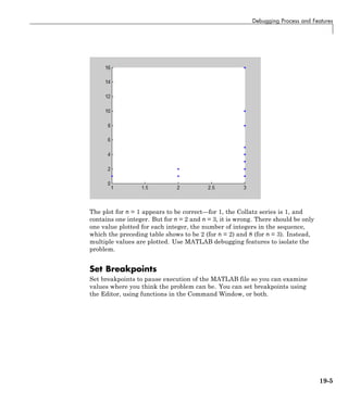
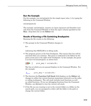
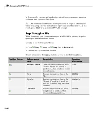
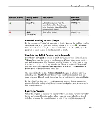
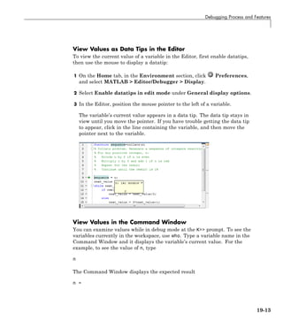
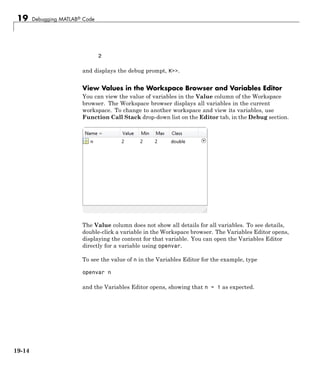
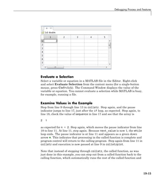
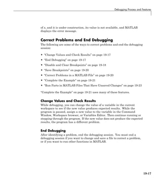
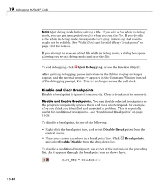
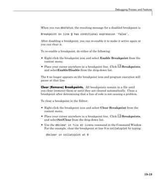
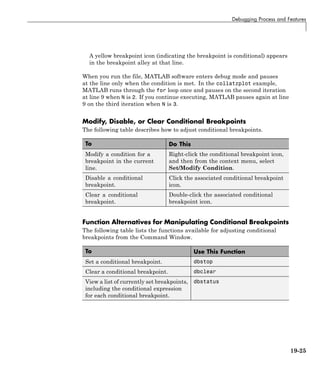
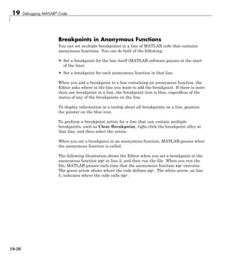
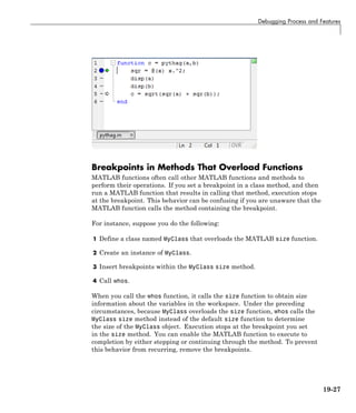
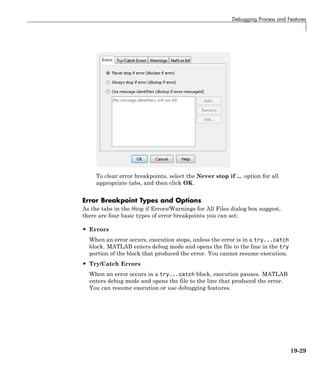
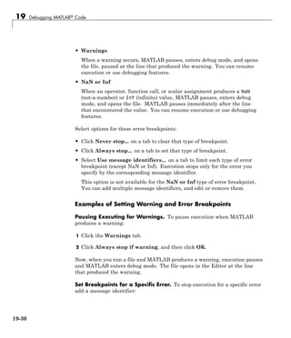
![Debugging Process and Features
1 Click the Errors, Try/Catch Errors, or Warnings tab.
2 Click Use Message Identifiers.
3 Click Add.
4 In the resulting Add Message Identifier dialog box, type the message
identifier of the error for which you want to stop. The identifier is of the form
component:message (for example, MATLAB:narginchk:notEnoughInputs).
Then click OK.
The message identifier you specified appears in the Stop if Errors/Warnings
for All Files dialog box.
5 Click OK.
Obtain Error Message Identifiers. To obtain an error message identifier
generated by a MATLAB function, run the function to produce the error, and
then call MExeption.last. For example:
surf
MException.last
The Command Window displays the MException object, including the error
message identifier in the identifier field. For this example, it displays:
ans =
MException
Properties:
identifier: 'MATLAB:narginchk:notEnoughInputs'
message: 'Not enough input arguments.'
cause: {}
stack: [1x1 struct]
Methods
Obtain Warning Message Identifiers. To obtain a warning message
identifier generated by a MATLAB function, run the function to produce the
warning. Then, run:
19-31](https://image.slidesharecdn.com/matlabprog-220902050722-ff974cdf/85/matlab_prog-pdf-591-320.jpg)
![19 Debugging MATLAB® Code
[m,id] = lastwarn
MATLAB returns the last warning identifier to id. An example of a warning
message identifier is MATLAB:concatenation:integerInteraction.
Function Alternative for Manipulating Error Breakpoints
The function equivalent for each option in the Stop if Errors/Warnings for
All Files dialog box, appears to the right of each option. For example, the
function equivalent for Always stop if error is dbstop if error. Use these
functions in the Command Window as listed in the following table.
To Use This Function
Set error breakpoints. dbstop
Clear error breakpoints. dbclear
View a list of currently set breakpoints,
including the condition and message identifier
for each error breakpoint.
dbstatus
19-32](https://image.slidesharecdn.com/matlabprog-220902050722-ff974cdf/85/matlab_prog-pdf-592-320.jpg)
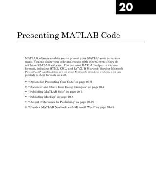
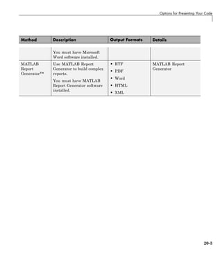
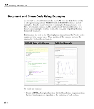
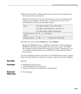
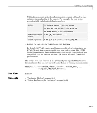
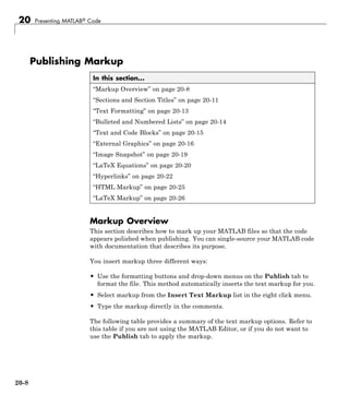
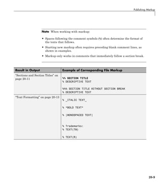

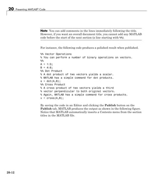
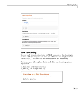
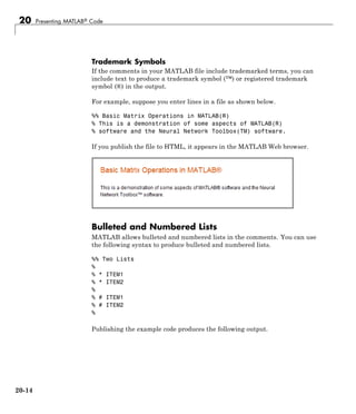
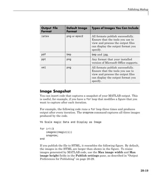
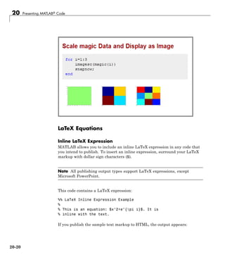
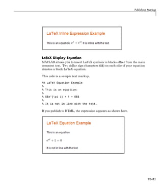
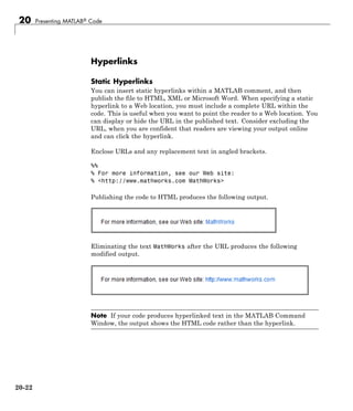
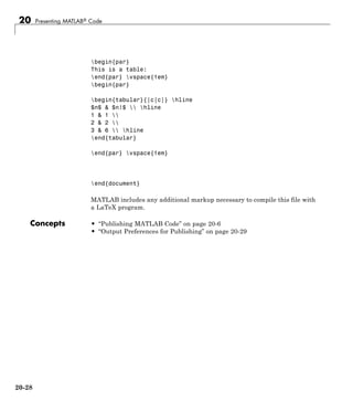
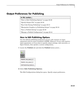
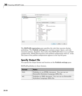
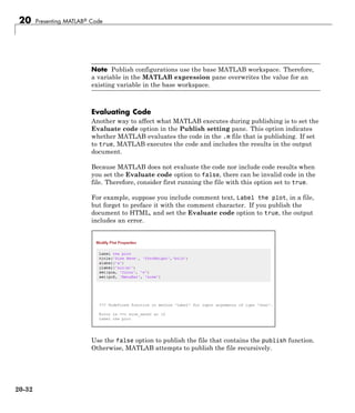
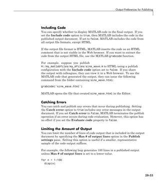
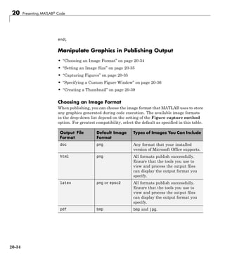
![20 Presenting MATLAB® Code
Use This Figure Capture
Method
To Get Figure Captures with These Appearance Details
Window Decorations Plot Backgrounds
entireGUIWindow Included for dialog boxes;
Excluded for figures
Set to white for figures;
matches the screen for dialog
boxes
print Excluded for dialog boxes and
figures
Set to white
getframe Excluded for dialog boxes and
figures
Matches the screen plot
background
entireFigureWindow Included for dialog boxes and
figures
Matches the screen plot
background
Note Typically, MATLAB figures have the HandleVisibility property set to
on. Dialog boxes are figures with the HandleVisibility property set to off or
callback. If your results are different from the results listed in the preceding
table, the HandleVisibility property of your figures or dialog boxes might
be atypical. For more information, see “HandleVisibility Property”.
Specifying a Custom Figure Window
MATLAB allows you to specify custom appearance for figures it creates. If
the Use new figure option in the Publish settings pane is set to true, then
in the published output, MATLAB uses a Figure window at the default size
and with a white background. If the Use new figure option is set to false,
then MATLAB uses the properties from an open Figure window to determine
the appearance of code-generated figures. This preference does not apply to
figures included using the syntax in “External Graphics” on page 20-16.
Use the following code as a template to produce Figure windows that meet
your needs.
% Create figure
figure1 = figure('Name','purple_background',...
'Color',[0.4784 0.06275 0.8941]);
20-36](https://image.slidesharecdn.com/matlabprog-220902050722-ff974cdf/85/matlab_prog-pdf-628-320.jpg)
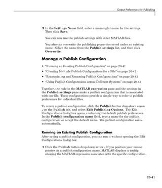
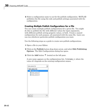
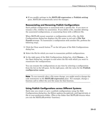
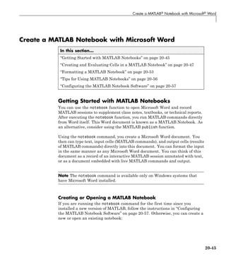
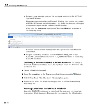
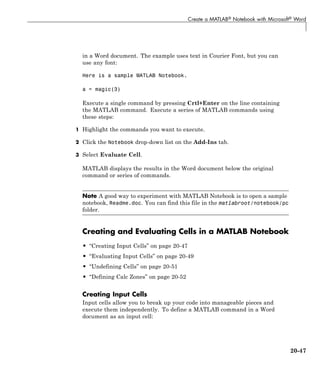
![20 Presenting MATLAB® Code
1 Type the command into the MATLAB Notebook as text. For example,
This is a sample MATLAB Notebook.
a = magic(3)
2 Position the cursor anywhere in the command, and then select Define Input
Cell from the Notebook drop-down list. If the command is embedded in a line
of text, use the mouse to select it. The characters appear within cell markers
([ ]). Cell markers are bold, gray brackets. They differ from the brackets
used to enclose matrices by their size and weight.
[a = magic(3)]
Creating Autoinit Input Cells. Autoinit cells are identical to input cells
with additional characteristics:
• Autoinit cells evaluate when MATLAB Notebook opens.
• Commands in autoinit cells display in dark blue characters.
To create an autoinit cell, highlight the text, and then select Define AutoInit
Cell from the Notebook drop-down list.
Creating Cell Groups. You can collect several input cells into a single input
cell, called a cell group. All the output from a cell group appears in a single
output cell immediately after the group. Cell groups are useful when you need
several MATLAB commands to execute in sequence. For instance, defining
labels and tick marks in a plot requires multiple commands:
x = -pi:0.1:pi;
plot(x,cos(x))
title('Sample Plot')
xlabel('x')
ylabel('cos(x)')
set(gca,'XTick',-pi:pi:pi)
set(gca,'XTickLabel',{'-pi','0','pi'})
To create a cell group:
1 Use the mouse to select the input cells that are to make up the group.
20-48](https://image.slidesharecdn.com/matlabprog-220902050722-ff974cdf/85/matlab_prog-pdf-640-320.jpg)
![Create a MATLAB® Notebook with Microsoft® Word
2 Select Group Cells from the Notebook drop-down list.
A single pair of cell markers now surrounds the new cell group.
[x = -pi:0.1:pi;
plot(x,cos(x))
title('Sample Plot')
xlabel('x')
ylabel('cos(x)')
set(gca,'XTick',-pi:pi:pi)
set(gca,'XTickLabel',{'-pi','0','pi'})]
When working with cell groups, you should note several behaviors:
• A cell group cannot contain output cells. If the selection includes output
cells, they are deleted.
• A cell group cannot contain text. If the selection includes text, the text
appears after the cell group, unless it precedes the first input cell in the
selection.
• If you select part or all of an output cell, the cell group includes the
respective input cell.
• If the first line of a cell group is an autoinit cell, then the entire group is
an autoinit cell.
Evaluating Input Cells
After you define a MATLAB command as an input cell, you can evaluate it in
your MATLAB Notebook using these steps:
1 Highlight or place your cursor in the input cell you want to evaluate.
2 Select Evaluate Cell in the Notebook drop-down list, or press Ctrl+Enter.
The notebook evaluates and displays the results in an output cell immediately
following the input cell. If there is already an output cell, its contents update
wherever the output cell appears in the notebook. For example:
This is a sample MATLAB Notebook.
[a = magic(3) ]
20-49](https://image.slidesharecdn.com/matlabprog-220902050722-ff974cdf/85/matlab_prog-pdf-641-320.jpg)
![20 Presenting MATLAB® Code
[a =
8 1 6
3 5 7
4 9 2 ]
To evaluate more than one MATLAB command contained in different, but
contiguous input cells:
1 Select a range of cells that includes the input cells you want to evaluate. You
can include text that surrounds input cells in your selection.
2 Select Evaluate Cell in the Notebook drop-down list or press Ctrl+Enter.
Note Text or numeric output always displays first, regardless of the order of
the commands in the group.
When each input cell evaluates, new output cells appear or existing ones are
replaced. Any error messages appear in red, by default.
Evaluating Cell Groups. Evaluate a cell group the same way you evaluate
an input cell (because a cell group is an input cell):
1 Position the cursor anywhere in the cell or in its output cell.
2 Select Evaluate Cell in the Notebook drop-down list or press Ctrl+Enter.
When MATLAB evaluates a cell group, the output for all commands in the
group appears in a single output cell. By default, the output cell appears
immediately after the cell group the first time the cell group is evaluated. If
you evaluate a cell group that has an existing output cell, the results appear
in that output cell, wherever it is located in the MATLAB Notebook.
Using a Loop to Evaluate Input Cells Repeatedly. MATLAB allows you
to evaluate a sequence of MATLAB commands repeatedly, using these steps:
1 Highlight the input cells, including any text or output cells located between
them.
20-50](https://image.slidesharecdn.com/matlabprog-220902050722-ff974cdf/85/matlab_prog-pdf-642-320.jpg)
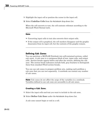
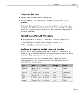
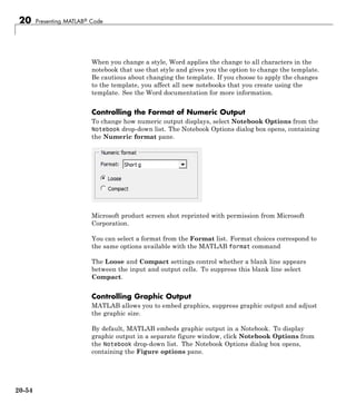
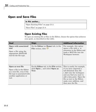
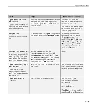
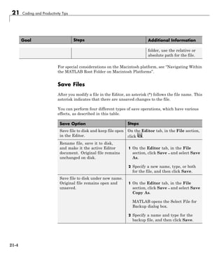
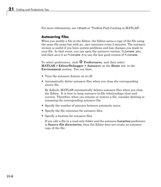
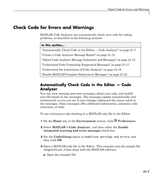
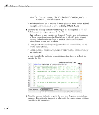
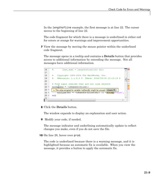
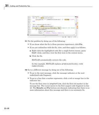
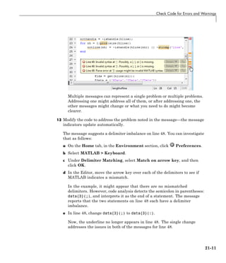
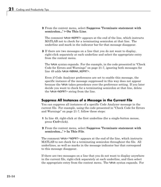
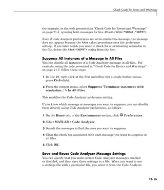
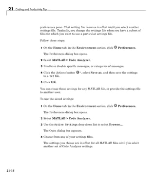
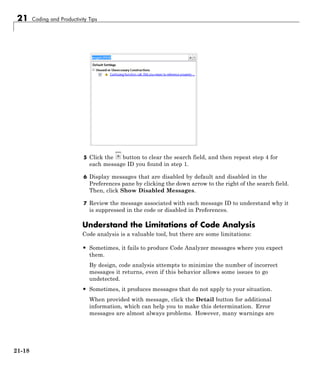
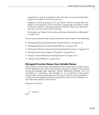
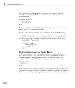
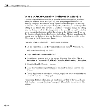
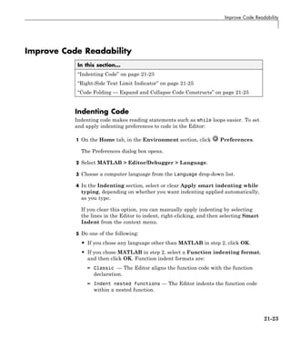
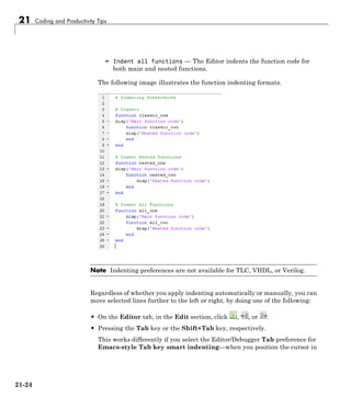
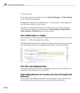
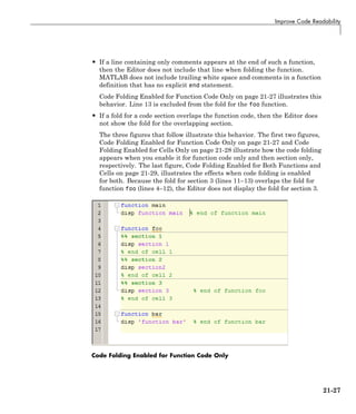
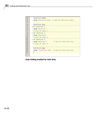
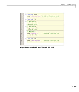
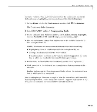
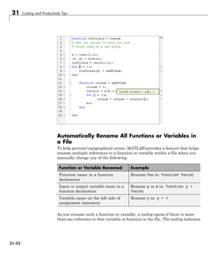
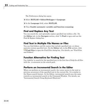
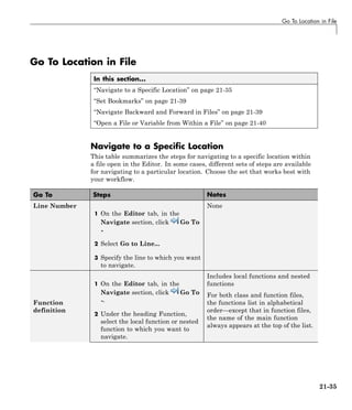
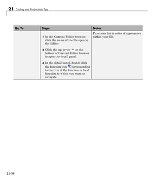
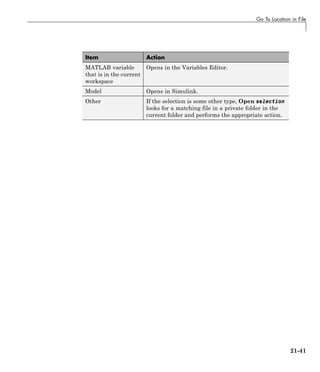
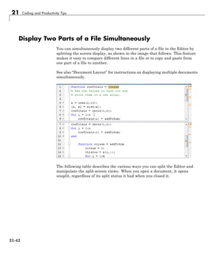
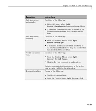
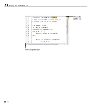
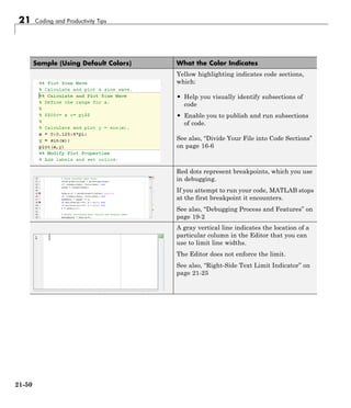
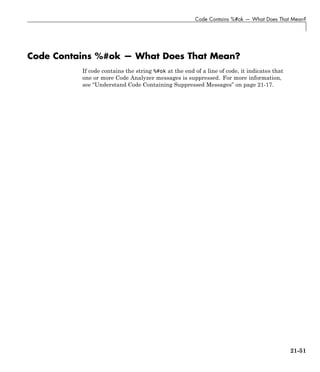
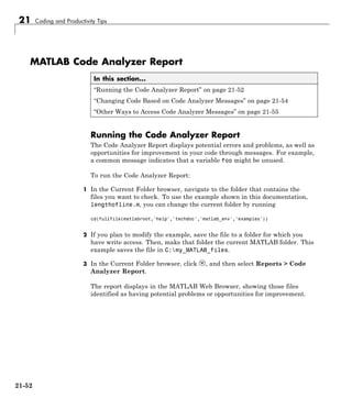
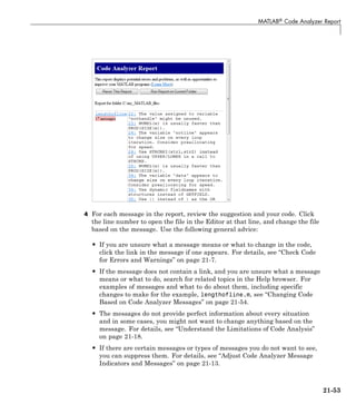
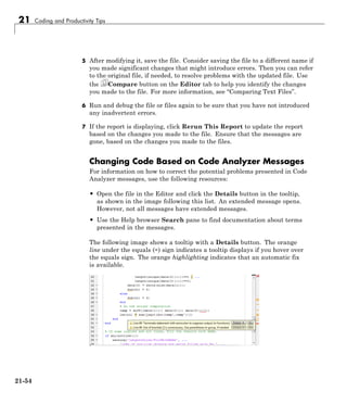
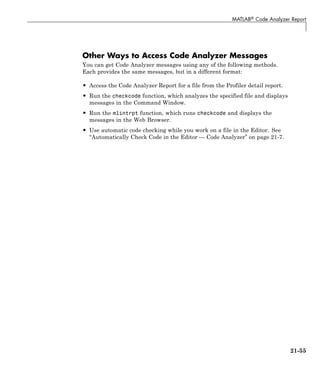
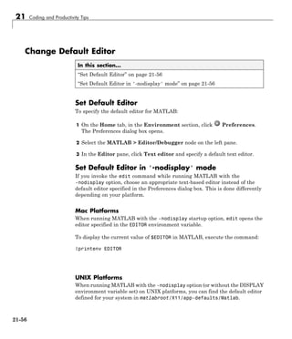

![22 Programming Utilities
Identify Program Dependencies
If you need to know what other functions and scripts your program is
dependent upon, use one of the techniques described below.
In this section...
“Simple Display of Program File Dependencies” on page 22-2
“Detailed Display of Program File Dependencies” on page 22-2
“Dependencies Within a Folder” on page 22-3
Simple Display of Program File Dependencies
For a simple display of all program files referenced by a particular function,
follow these steps:
1 Type clear functions to clear all functions from memory (see Note below).
Note clear functions does not clear functions locked by mlock. If you
have locked functions (which you can check using inmem) unlock them with
munlock, and then repeat step 1.
2 Execute the function you want to check. Note that the function arguments
you choose to use in this step are important, because you can get different
results when calling the same function with different arguments.
3 Type inmem to display all program files that were used when the function ran.
If you want to see what MEX-files were used as well, specify an additional
output:
[mfiles, mexfiles] = inmem
Detailed Display of Program File Dependencies
For a more detailed display of dependent function information, use the
matlab.codetools.requiredFilesAndProducts function. In addition to
program files, matlab.codetools.requiredFilesAndProducts shows which
22-2](https://image.slidesharecdn.com/matlabprog-220902050722-ff974cdf/85/matlab_prog-pdf-710-320.jpg)
![Identify Program Dependencies
MathWorks products a particular function depends on. If you have a function,
myFun, that calls to the edge function in the Image Processing Toolbox™:
[fList,pList] = matlab.codetools.requiredFilesAndProducts('myFun.m');
fList
fList =
'C:workmyFun.m'
The only required program file, is the function file itself, myFun.
{pList.Name}'
ans =
'MATLAB'
'Image Processing Toolbox'
The file, myFun.m, requires both MATLAB and the Image Processing Toolbox.
Dependencies Within a Folder
The Dependency Report shows dependencies among MATLAB code files in a
folder. Use this report to determine:
• Which files in the folder are required by other files in the folder
• If any files in the current folder will fail if you delete a file
• If any called files are missing from the current folder
The report does not list:
• Files in the toolbox/matlab folder because every MATLAB user has those
files.
Therefore, if you use a function file that shadows a built-in function file,
MATLAB excludes both files from the list.
• Files called from anonymous functions.
• The superclass for a class file.
22-3](https://image.slidesharecdn.com/matlabprog-220902050722-ff974cdf/85/matlab_prog-pdf-711-320.jpg)
![22 Programming Utilities
pcode *.m
See the pcode function reference page for a description of all syntaxes for
generating P-code files.
Invoking the P-Code File
You invoke the resulting P-code file in the same way you invoke the MATLAB
.m source file from which it was derived. For example, to invoke file myfun.p,
type
[out, out2, ...] = myfun(in1, in2, ...);
To invoke script myscript.p, type
myscript;
When you call a P-code file, MATLAB gives it execution precedence over its
corresponding .m source file. This is true even if you happen to change the
source code at some point after generating the P-code file. Remember to
remove the .m source file before distributing your code.
Running Older P-Code Files on Later Versions of MATLAB
P-code files are designed to be independent of the release under which they
were created and the release in which they are used (backward and forward
compatibility). New and deprecated MATLAB features can be a problem, but
it is the same problem that would exist if you used the original MATLAB
input file. To fix errors of this kind in a P-code file, fix the corresponding
MATLAB input file and create a new P-code file.
P-code files built using MATLAB Version 7.4 and earlier have a different
format than those built with more recent versions of MATLAB. You still can
use these older P-code files when you run MATLAB 7.4 and later, but this
capability could be removed in a future release. MathWorks recommends that
you rebuild any P-code files that were built with MATLAB 7.4 or earlier using
a more recent version of MATLAB, and then redistribute them as necessary.
22-10](https://image.slidesharecdn.com/matlabprog-220902050722-ff974cdf/85/matlab_prog-pdf-718-320.jpg)
![Create Hyperlinks that Run Functions
Some symbols might not be interpreted correctly and you might need to use
the ASCII value for the symbol. For example, an alternative way to run the
previous statement is to use ASCII 62 instead of the greater than symbol:
disp('<a href="matlab:str=[''Value '' char(62) '' 0'']">Positive</a>')
22-15](https://image.slidesharecdn.com/matlabprog-220902050722-ff974cdf/85/matlab_prog-pdf-723-320.jpg)


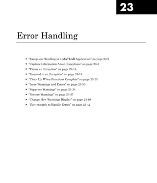
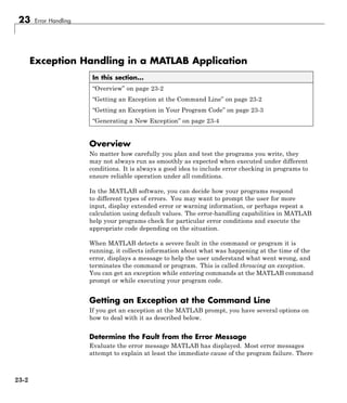
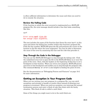
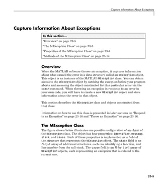
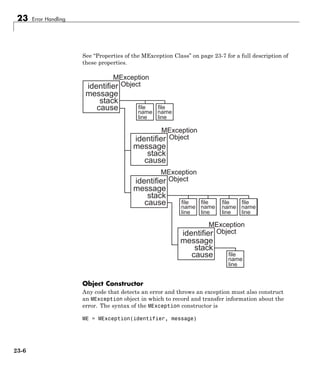
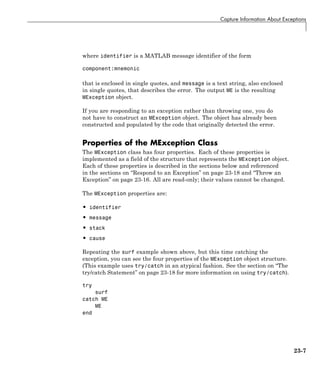
![23 Error Handling
Run this at the command line and MATLAB returns the contents of the
MException object:
ME =
MException object with properties:
identifier: 'MATLAB:narginchk:notEnoughInputs'
message: 'Not enough input arguments.'
stack: [1x1 struct]
cause: {}
The stack field shows the filename, function, and line number where the
exception was thrown:
ME.stack
ans =
file: 'matlabroottoolboxmatlabgraph3dsurf.m'
name: 'surf'
line: 54
The cause field is empty in this case. Each field is described in more detail
in the sections that follow.
Message Identifiers
A message identifier is a tag that you attach to an error or warning statement
that makes that error or warning uniquely recognizable by MATLAB. You can
use message identifiers with error reporting to better identify the source of
an error, or with warnings to control any selected subset of the warnings in
your programs.
The message identifier is a read-only character string that specifies a
component and a mnemonic label for an error or warning. The format of
a simple identifier is
component:mnemonic
A colon separates the two parts of the identifier: component and mnemonic.
If the identifier uses more than one component, then additional colons are
required to separate them. A message identifier must always contain at
least one colon.
23-8](https://image.slidesharecdn.com/matlabprog-220902050722-ff974cdf/85/matlab_prog-pdf-734-320.jpg)
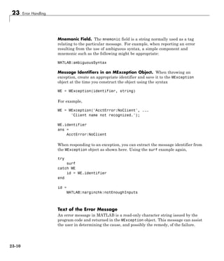
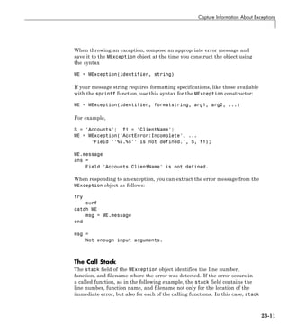
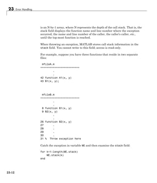
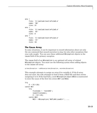
![23 Error Handling
'Unable to load from file %s', filename);
ME3 = addCause(ME3, ME1);
ME3 = addCause(ME3, ME2);
end
end
There are two exceptions in the cause field of ME3:
ME3.cause
ans =
[1x1 MException]
[1x1 MException]
Examine the cause field of ME3 to see the related errors:
ME3.cause{:}
ans =
MException object with properties:
identifier: 'MATLAB:UndefinedFunction'
message: 'Undefined function or method 'D' for input
arguments of type 'double'.'
stack: [0x1 struct]
cause: {}
ans =
MException object with properties:
identifier: 'MATLAB:load:couldNotReadFile'
message: 'Unable to read file test204: No such file or
directory.'
stack: [0x1 struct]
cause: {}
Methods of the MException Class
There are ten methods that you can use with the MException class. The
names of these methods are case-sensitive. See the MATLAB function
reference pages for more information.
23-14](https://image.slidesharecdn.com/matlabprog-220902050722-ff974cdf/85/matlab_prog-pdf-740-320.jpg)
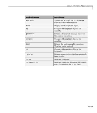
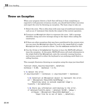
![Throw an Exception
err = addCause(err, errCause);
end
% 4) Throw the exception to stop execution and display
an error message.
throw(err)
end
If the program detects the OutOfRange condition, the throw(err) statement
throws an exception at the end. If the BadInput condition is also detected, the
program also displays this as the cause:
resultsArr = [1.63, 2.05, 0.91, 2.16, 1.5, 2.11 0.72];
check_results(resultsArr, 'run33.dat')
Error using check_results (line 20)
Resulting value is outside expected range
Caused by:
Input file run33.dat is out of date.
23-17](https://image.slidesharecdn.com/matlabprog-220902050722-ff974cdf/85/matlab_prog-pdf-743-320.jpg)
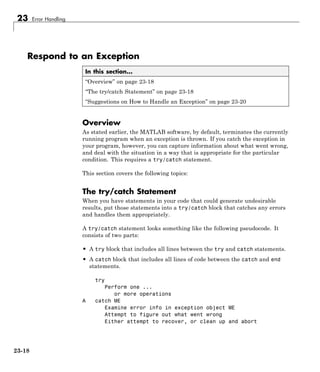
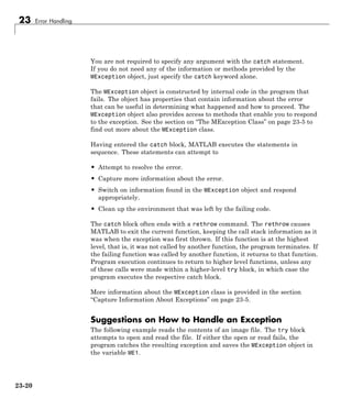
![Respond to an Exception
The catch block in the example checks to see if the specified file could not be
found. If so, the program allows for the possibility that a common variation
of the filename extension (e.g., jpeg instead of jpg) was used by retrying
the operation with a modified extension. This is done using a try/catch
statement nested within the original try/catch.
function d_in = read_image(filename)
[path name ext] = fileparts(filename);
try
fid = fopen(filename, 'r');
d_in = fread(fid);
catch ME1
% Get last segment of the error message identifier.
idSegLast = regexp(ME1.identifier, '(?<=:)w+$', 'match');
% Did the read fail because the file could not be found?
if strcmp(idSegLast, 'InvalidFid') && ...
~exist(filename, 'file')
% Yes. Try modifying the filename extension.
switch ext
case '.jpg' % Change jpg to jpeg
filename = strrep(filename, '.jpg', '.jpeg')
case '.jpeg' % Change jpeg to jpg
filename = strrep(filename, '.jpeg', '.jpg')
case '.tif' % Change tif to tiff
filename = strrep(filename, '.tif', '.tiff')
case '.tiff' % Change tiff to tif
filename = strrep(filename, '.tiff', '.tif')
otherwise
fprintf('File %s not foundn', filename);
rethrow(ME1);
end
% Try again, with modifed filenames.
try
fid = fopen(filename, 'r');
d_in = fread(fid);
catch ME2
fprintf('Unable to access file %sn', filename);
23-21](https://image.slidesharecdn.com/matlabprog-220902050722-ff974cdf/85/matlab_prog-pdf-747-320.jpg)
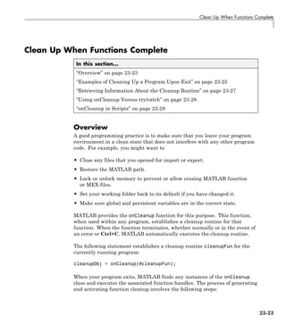
![Clean Up When Functions Complete
Examples of Cleaning Up a Program Upon Exit
Example 1 — Close Open Files on Exit
MATLAB closes the file with identifier fid when function openFileSafely
terminates:
function openFileSafely(fileName)
fid = fopen(fileName, 'r');
c = onCleanup(@()fclose(fid));
s = fread(fid);
.
.
.
end
Example 2 — Maintain the Selected Folder
This example preserves the current folder whether functionThatMayError
returns an error or not:
function changeFolderSafely(fileName)
currentFolder = pwd;
c = onCleanup(@()cd(currentFolder));
functionThatMayError;
end % c executes cd(currentFolder) here.
Example 3 — Close Figure and Restore MATLAB Path
This example extends the MATLAB path to include files in the toolboximages
folders, and then displays a figure from one of these folders. After the figure
displays, the cleanup routine restore_env closes the figure and restores
the path to its original state:
function showImageOutsidePath(imageFile)
fig1 = figure;
imgpath = genpath([matlabroot 'toolboximages']);
23-25](https://image.slidesharecdn.com/matlabprog-220902050722-ff974cdf/85/matlab_prog-pdf-751-320.jpg)
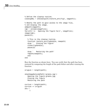
![Clean Up When Functions Complete
Retrieving Information About the Cleanup Routine
In Example 3 shown above, the cleanup routine and data needed to call it are
contained in a handle to an anonymous function:
@()restore_env(fig1, imgpath)
The details of that handle are then contained within the object returned by
the onCleanup function:
cleanupObj = onCleanup(@()restore_env(fig1, imgpath));
You can access these details using the task property of the cleanup object
as shown here. (Modify the showImageOutsidePath function by adding the
following code just before the comment line that says, “% This is the
cleanup routine.”)
disp ' Displaying information from the function handle:'
task = cleanupObj.task;
fun = functions(task)
wsp = fun.workspace{2,1}
fprintf('n');
pause(2);
Run the modified function to see the output of the functions command and
the contents of one of the workspace cells:
showImageOutsidePath('greens.jpg')
Opening the figure greens.jpg
Displaying information from the function handle:
fun =
function: '@()restore_env(fig1,imgpath)'
type: 'anonymous'
file: 'c:workg6.m'
workspace: {2x1 cell}
wsp =
imageFile: 'greens.jpg'
fig1: 1
imgpath: [1x3957 char]
cleanupObj: [1x1 onCleanup]
rgb: [300x500x3 uint8]
23-27](https://image.slidesharecdn.com/matlabprog-220902050722-ff974cdf/85/matlab_prog-pdf-753-320.jpg)
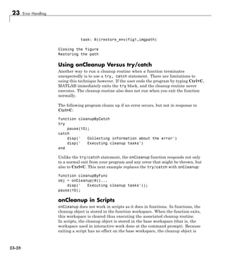
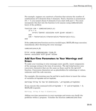
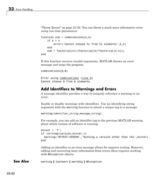
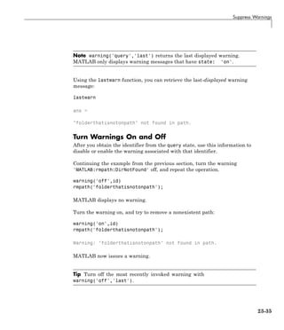
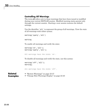
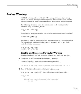
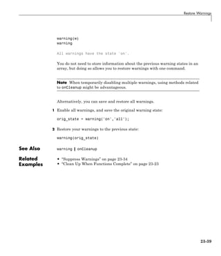
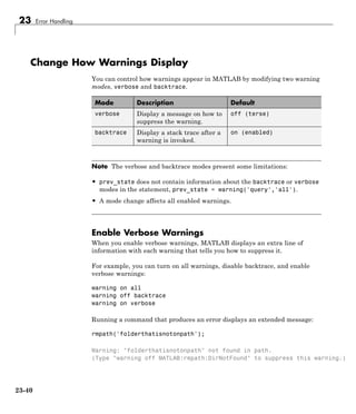
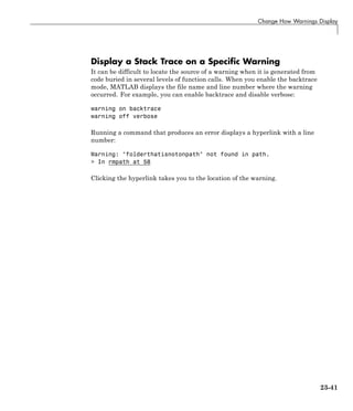
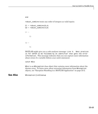


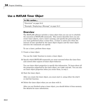
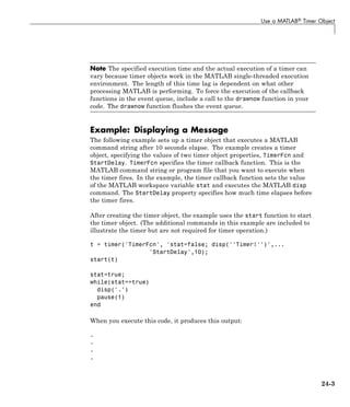
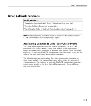
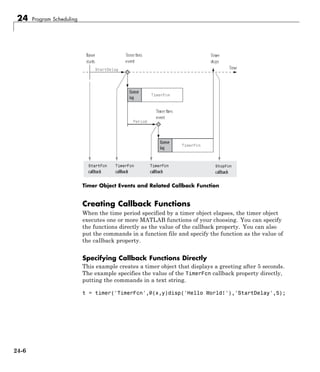
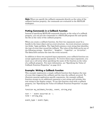
![24 Program Scheduling
event_time = datestr(event.Data.time);
msg = [event_type txt1 event_time];
disp(msg)
disp(txt2)
Specifying the Value of Callback Function Properties
You associate a callback function with a specific event by setting the value of
the appropriate callback property. You can specify the callback function as
a cell array or function handle. If your callback function accepts additional
arguments, you must use a cell array.
The following table shows the syntax for several sample callback functions
and describes how you call them.
Callback Function Syntax
How to Specify as a Property
Value for Object t
function myfile(obj, event) t.StartFcn = @myfile
function myfile t.StartFcn = @(~,~)myfile
function myfile(obj, event,
arg1, arg2)
t.StartFcn = {@myfile, 5, 6}
This example illustrates several ways you can specify the value of timer object
callback function properties, some with arguments and some without. To see
the code of the callback function, my_callback_fcn, see “Example: Writing
a Callback Function” on page 24-7:
1 Create a timer object.
t = timer('StartDelay', 4, 'Period', 4, 'TasksToExecute', 2, ...
'ExecutionMode', 'fixedRate');
2 Specify the value of the StartFcn callback. Note that the example specifies
the value in a cell array because the callback function needs to access
arguments passed to it:
t.StartFcn = {@my_callback_fcn, 'My start message'};
24-8](https://image.slidesharecdn.com/matlabprog-220902050722-ff974cdf/85/matlab_prog-pdf-778-320.jpg)
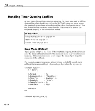
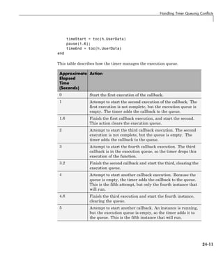
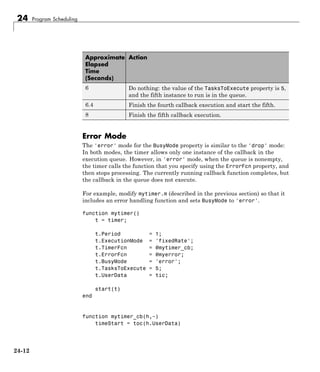
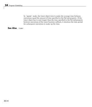
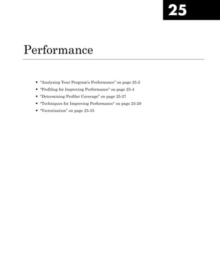
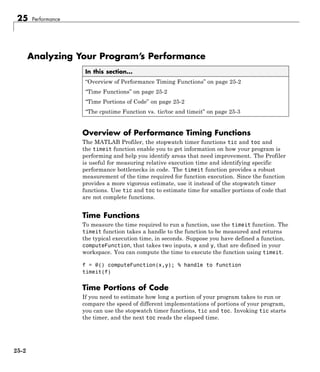

![Profiling for Improving Performance
• “Running the Profiler” on page 25-7
• “Profiling a Graphical User Interface” on page 25-8
• “Profiling Statements from the Command Window” on page 25-9
• “Changing Fonts for the Profiler” on page 25-9
• “Troubleshooting” on page 25-9
For information about the reports generated by the Profiler, see “Profile
Summary Report” on page 25-12 and “Profile Detail Report” on page 25-14.
Running the Profiler
To profile a MATLAB code file or a line of code:
1 Launch the Profiler using one of the following methods:
• On the Editor tab, in the Run section, click Run and Time. If you use
this method, the Profiler automatically profiles the code in the current
Editor tab, so skip to step 5.
• On the Home tab, in the Code section, click Run and Time.
• In the Command Window, type profile viewer.
2 Do one of the following in the Profiler:
• For a statement you have not profiled in the current MATLAB session:
In the Run this code field, type the statement you want to run.
For example, you can run the Lotka-Volterra example, which is provided
with MATLAB examples (lotkademo):
[t,y] = ode23('lotka',[0 2],[20;20])
• For a statement you previously profiled in the current MATLAB session:
1 Select the statement from the list box—MATLAB automatically starts
profiling the code.
2 Skip to step 5.
25-7](https://image.slidesharecdn.com/matlabprog-220902050722-ff974cdf/85/matlab_prog-pdf-791-320.jpg)
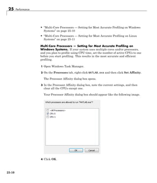
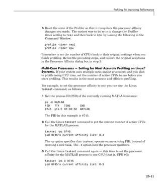
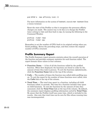
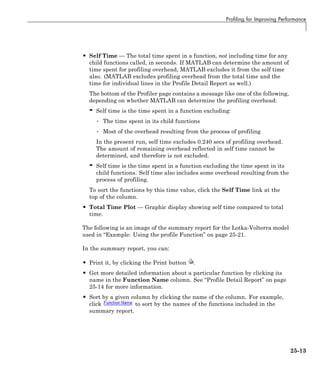
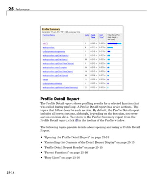
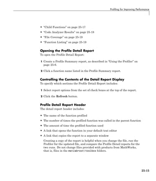
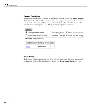
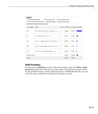
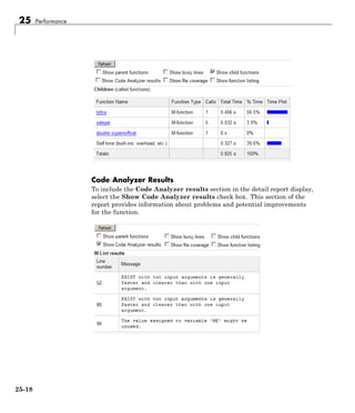
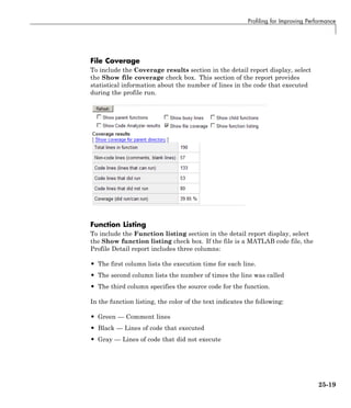
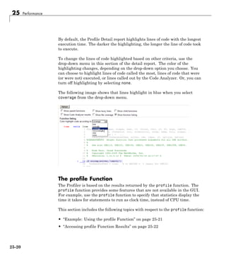
![Profiling for Improving Performance
• “Saving profile Function Reports” on page 25-24
• “Using the profile Function to Change the Time Type Used by the Profiler”
on page 25-25
Example: Using the profile Function
This example demonstrates how to run profile:
1 To start profile, type the following in the Command Window:
profile on
2 Execute a MATLAB code file. This example runs the Lotka-Volterra
predator-prey population model. For more information about this model, type
lotkademo, which runs a demonstration.
[t,y] = ode23('lotka',[0 2],[20;20]);
3 Generate the profile report and display it in the Profiler window. This
suspends profile.
profile viewer
4 Restart profile, without clearing the existing statistics.
profile resume
The profile function is now ready to continue gathering statistics for
any more files you run. It will add these new statistics to those statistics
generated in the previous steps.
5 Stop profile when you finish gathering statistics.
profile off
6 To view the profile data, call profile specifying the 'info' argument. The
profile function returns data in a structure.
p = profile('info')
p =
25-21](https://image.slidesharecdn.com/matlabprog-220902050722-ff974cdf/85/matlab_prog-pdf-805-320.jpg)
![25 Performance
FunctionTable: [33x1 struct]
FunctionHistory: [2x0 double]
ClockPrecision: 1.0000e-03
ClockSpeed: 3.0000e+09
Name: 'MATLAB'
Overhead: 0
The FunctionTable indicates that statistics were gathered for 33 functions.
7 To save the profile report, use the profsave function. This function stores
the profile information in separate HTML files, for each function listed in
FunctionTable of p.
profsave(p)
By default, profsave puts these HTML files in a subfolder of the current
folder named profile_results, and displays the summary report in your
system browser. You can specify another folder name as an optional second
argument to profsave.
Accessing profile Function Results
The profile function returns results in a structure. This example illustrates
how you can access these results:
1 To start profile, specifying the history option, type the following in the
Command Window:
profile on -history
The history option specifies that the report include information about the
sequence of functions as they are entered and exited during profiling.
2 Execute a MATLAB code file. This example runs the Lotka-Volterra
predator-prey population model. For more information about this model, type
lotkademo, which runs a demonstration.
[t,y] = ode23('lotka',[0 2],[20;20]);
3 Stop profiling.
25-22](https://image.slidesharecdn.com/matlabprog-220902050722-ff974cdf/85/matlab_prog-pdf-806-320.jpg)
![Profiling for Improving Performance
profile off
4 Get the structure containing profile results.
stats = profile('info')
stats =
FunctionTable: [33x1 struct]
FunctionHistory: [2x880 double]
ClockPrecision: 1.0000e-03
ClockSpeed: 3.0000e+09
Name: 'MATLAB'
Overhead: 0
5 The FunctionTable field is an array of structures, where each structure
represents a MATLAB function (M-function), MATLAB local function,
MEX-function, or, because the builtin option is specified, a MATLAB built-in
function.
stats.FunctionTable
ans =
33x1 struct array with fields:
CompleteName
FunctionName
FileName
Type
Children
Parents
ExecutedLines
IsRecursive
TotalRecursiveTime
PartialData
NumCalls
TotalTime
6 View the second structure in FunctionTable.
stats.FunctionTable(2)
25-23](https://image.slidesharecdn.com/matlabprog-220902050722-ff974cdf/85/matlab_prog-pdf-807-320.jpg)
![25 Performance
ans =
CompleteName: [1x95 char]
FunctionName: 'ode23'
FileName: [1x89 char]
Type: 'M-function'
Children: [6x1 struct]
Parents: [0x1 struct]
ExecutedLines: [139x3 double]
IsRecursive: 0
TotalRecursiveTime: 0
PartialData: 0
NumCalls: 1
TotalTime: 0.0920
7 To view the history data generated by profile, view the FunctionHistory,
for example, stats.FunctionHistory. The history data is a 2-by-n array.
The first row contains Boolean values, where 0 (zero) means entrance into
a function and 1 means exit from a function. The second row identifies the
function being entered or exited by its index in the FunctionTable field. To
see how to create a formatted display of history data, see the example on
the profile reference page.
Saving profile Function Reports
To save the profile report, use the profsave function.
This function stores the profile information in separate HTML files, for each
function listed in the FunctionTable field of the structure, stats.
profsave(stats)
By default, profsave puts these HTML files in a subfolder of the current
folder named profile_results. You can specify another folder name as an
optional second argument to profsave.
profsave(stats,'mydir')
25-24](https://image.slidesharecdn.com/matlabprog-220902050722-ff974cdf/85/matlab_prog-pdf-808-320.jpg)
![Profiling for Improving Performance
Using the profile Function to Change the Time Type Used by
the Profiler
By default, MATLAB generates the Profiler Summary report using CPU time,
as opposed to real (wall clock) time. This example illustrates how you can
direct MATLAB to use real time instead.
Specify that the Profiler use real time instead, by using the profile function
with the -timer real option, as shown in this example:
1 If the Profiler is currently open, close the Profiler, and if prompted, stop
profiling.
2 Set the timer to real time by typing the following in the Command Window:
profile on -timer real
3 Run the file that you want to profile. This example runs the Lotka-Volterra
predator-prey population model.
[t,y] = ode23('lotka',[0 2],[20;20]);
4 Open the Profiler by typing the following in the Command Window:
profile viewer
The Profiler opens and indicates that it is using real time, as shown in the
following image.
5 To change the timer back to using CPU time:
25-25](https://image.slidesharecdn.com/matlabprog-220902050722-ff974cdf/85/matlab_prog-pdf-809-320.jpg)
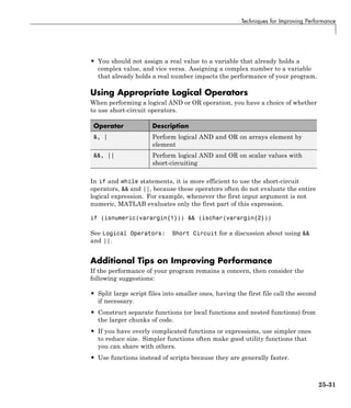
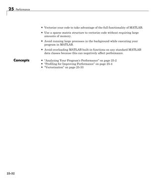
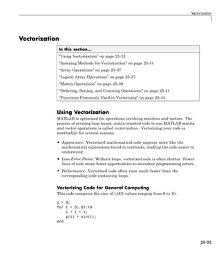
![Vectorization
Subscripted Indexing
In subscripted indexing, the index values indicate their position within
the matrix. Thus, if A = 6:10, then A([3 5]) denotes the third and fifth
elements of vector A:
A = 6:10;
A([3 5])
ans =
8 10
Multidimensional arrays or matrices use multiple index parameters for
subscripted indexing.
A = [11 12 13; 14 15 16; 17 18 19]
A(2:3,2:3)
A =
11 12 13
14 15 16
17 18 19
ans =
15 16
18 19
Linear Indexing
In linear indexing, MATLAB assigns every element of a matrix a single index
as if the entire matrix structure stretches out into one column vector.
A = [11 12 13; 14 15 16; 17 18 19];
A(6)
A([3,1,8])
A([3;1;8])
25-35](https://image.slidesharecdn.com/matlabprog-220902050722-ff974cdf/85/matlab_prog-pdf-819-320.jpg)
![25 Performance
ans =
18
ans =
17 11 16
ans =
17
11
16
In the previous example, the returned matrix elements preserve the shape
specified by the index parameter. If the index parameter is a row vector,
MATLAB returns the specified elements as a row vector.
Note Use the functions sub2ind and ind2sub to convert between subscripted
and linear indices.
Logical Indexing
With logical indexing, the index parameter is a logical matrix that is the same
size as A and contains only 0s and 1s.
MATLAB selects elements of A that contain a 1 in the corresponding position
of the logical matrix:
A = [11 12 13; 14 15 16; 17 18 19];
A(logical([0 0 1; 0 1 0; 1 1 1]))
ans =
17
15
25-36](https://image.slidesharecdn.com/matlabprog-220902050722-ff974cdf/85/matlab_prog-pdf-820-320.jpg)
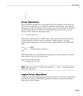
![25 Performance
For example, suppose while collecting data from 10,000 cones, you record
several negative values for the diameter. You can determine which values in
a vector are valid with the >= operator:
D = [-0.2 1.0 1.5 3.0 -1.0 4.2 3.14];
D >= 0
ans =
0 1 1 1 0 1 1
You can directly exploit the logical indexing power of MATLAB to select the
valid cone volumes, Vgood, for which the corresponding elements of D are
nonnegative:
Vgood = V(D >= 0);
MATLAB allows you to perform a logical AND or OR on the elements of an
entire vector with the functions all and any, respectively. You can throw a
warning if all values of D are below zero:
if all(D < 0)
warning('All values of diameter are negative.');
return;
end
MATLAB can compare two vectors of the same size, allowing you to impose
further restrictions. This code finds all the values where V is nonnegative
and D is greater than H:
V((V >= 0) & (D > H))
The resulting vector is the same size as the inputs.
To aid comparison, MATLAB contains special values to denote overflow,
underflow, and undefined operators, such as inf and nan. Logical operators
isinf and isnan exist to help perform logical tests for these special values.
For example, it is often useful to exclude NaN values from computations:
x = [2 -1 0 3 NaN 2 NaN 11 4 Inf];
xvalid = x(~isnan(x))
25-38](https://image.slidesharecdn.com/matlabprog-220902050722-ff974cdf/85/matlab_prog-pdf-822-320.jpg)
![Vectorization
xvalid =
2 -1 0 3 2 11 4 Inf
Note Inf == Inf returns true; however, NaN == NaN always returns false.
Matrix Operations
Matrix operations act according to the rules of linear algebra. These
operations are most useful in vectorization if you are working with
multidimensional data.
Suppose you want to evaluate a function, F, of two variables, x and y.
F(x,y) = x*exp(-x2
- y2
)
To evaluate this function at every combination of points in the x and y, you
need to define a grid of values:
x = -2:0.2:2;
y = -1.5:0.2:1.5;
[X,Y] = meshgrid(x,y);
F = X.*exp(-X.^2-Y.^2);
Without meshgrid, you might need to write two for loops to iterate through
vector combinations. The function ndgrid also creates number grids from
vectors, but can construct grids beyond three dimensions. meshgrid can only
construct 2-D and 3-D grids.
In some cases, using matrix multiplication eliminates intermediate steps
needed to create number grids:
x = -2:2;
y = -1:0.5:1;
x'*y
ans =
2.0000 1.0000 0 -1.0000 -2.0000
25-39](https://image.slidesharecdn.com/matlabprog-220902050722-ff974cdf/85/matlab_prog-pdf-823-320.jpg)
![25 Performance
1.0000 0.5000 0 -0.5000 -1.0000
0 0 0 0 0
-1.0000 -0.5000 0 0.5000 1.0000
-2.0000 -1.0000 0 1.0000 2.0000
Constructing Matrices
When vectorizing code, you often need to construct a matrix with a particular
size or structure. Techniques exist for creating uniform matrices. For
instance, you might need a 5-by-5 matrix of equal elements:
A = ones(5,5)*10;
Or, you might need a matrix of repeating values:
v = 1:5;
A = repmat(v,3,1)
A =
1 2 3 4 5
1 2 3 4 5
1 2 3 4 5
The function repmat possesses flexibility in building matrices from smaller
matrices or vectors. repmat creates matrices by repeating an input matrix:
A = repmat(1:3,5,2)
B = repmat([1 2; 3 4],2,2)
A =
1 2 3 1 2 3
1 2 3 1 2 3
1 2 3 1 2 3
1 2 3 1 2 3
1 2 3 1 2 3
B =
1 2 1 2
25-40](https://image.slidesharecdn.com/matlabprog-220902050722-ff974cdf/85/matlab_prog-pdf-824-320.jpg)
![Vectorization
3 4 3 4
1 2 1 2
3 4 3 4
The bsxfun function provides a way of combining matrices of different
dimensions. Suppose that matrix A represents test scores, the rows of which
denote different classes. You want to calculate the difference between the
average score and individual scores for each class. Your first thought might
be to compute the simple difference, A - mean(A). However, MATLAB throws
an error if you try this code because the matrices are not the same size.
Instead, bsxfun performs the operation without explicitly reconstructing the
input matrices so that they are the same size.
A = [97 89 84; 95 82 92; 64 80 99;76 77 67;...
88 59 74; 78 66 87; 55 93 85];
dev = bsxfun(@minus,A,mean(A))
dev =
18 11 0
16 4 8
-15 2 15
-3 -1 -17
9 -19 -10
-1 -12 3
-24 15 1
Ordering, Setting, and Counting Operations
In many applications, calculations done on an element of a vector depend on
other elements in the same vector. For example, a vector, x, might represent a
set. How to iterate through a set without a for or while loop is not obvious.
The process becomes much clearer and the syntax less cumbersome when
you use vectorized code.
Eliminating Redundant Elements
A number of different ways exist for finding the redundant elements of a
vector. One way involves the function diff. After sorting the vector elements,
equal adjacent elements produce a zero entry when you use the diff function
on that vector. Because diff(x) produces a vector that has one fewer element
25-41](https://image.slidesharecdn.com/matlabprog-220902050722-ff974cdf/85/matlab_prog-pdf-825-320.jpg)
![25 Performance
than x, you must add an element that is not equal to any other element in the
set. NaN always satisfies this condition. Finally, you can use logical indexing
to choose the unique elements in the set:
x = [2 1 2 2 3 1 3 2 1 3];
x = sort(x);
difference = diff([x,NaN]);
y = x(difference~=0)
y =
1 2 3
Alternatively, you could accomplish the same operation by using the unique
function:
y=unique(x);
However, the unique function might provide more functionality than is
needed and slow down the execution of your code. Use the tic and toc
functions if you want to measure the performance of each code snippet.
Counting Elements in a Vector
Rather than merely returning the set, or subset, of x, you can count the
occurrences of an element in a vector. After the vector sorts, you can use the
find function to determine the indices of zero values in diff(x) and to show
where the elements change value. The difference between subsequent indices
from the find function indicates the number of occurrences for a particular
element:
x = [2 1 2 2 3 1 3 2 1 3];
x = sort(x);
difference = diff([x,max(x)+1]);
count = diff(find([1,difference]))
y = x(find(difference))
count =
3 4 3
25-42](https://image.slidesharecdn.com/matlabprog-220902050722-ff974cdf/85/matlab_prog-pdf-826-320.jpg)
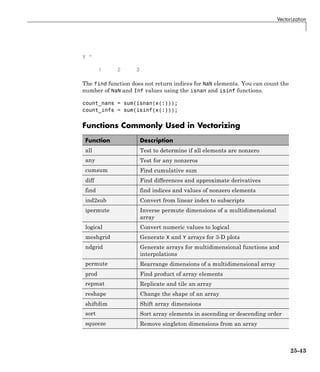

![Memory Allocation
If you remove elements from an existing array, MATLAB keeps the memory
storage contiguous by removing the deleted elements, and then compacting its
storage in the original memory location.
Working with Large Data Sets. If you are working with large data sets,
you need to be careful when increasing the size of an array to avoid getting
errors caused by insufficient memory. If you expand the array beyond the
available contiguous memory of its original location, MATLAB must make a
copy of the array and set this copy to the new value. During this operation,
there are two copies of the original array in memory. This temporarily doubles
the amount of memory required for the array and increases the risk of your
program running out of memory during execution. It is better to preallocate
sufficient memory for the largest potential size of the array at the start. See
“Preallocating Arrays” on page 25-29.
Copying Arrays
Internally, multiple variables can point to the same block of data, thus
sharing that array’s value. When you copy a variable to another variable (e.g.,
B = A), MATLAB makes a copy of the array reference, but not the array itself.
As long as you do not modify the contents of the array, there is no need to
store more than one copy of it. If you do modify any elements of the array,
MATLAB makes a copy of the array and then modifies that copy.
The following example demonstrates this. Start by creating a simple script
memUsed.m to display how much memory is currently being used by your
MATLAB process. Put these two lines of code in the script:
[usr, sys] = memory;
usr.MemUsedMATLAB
Get an initial reading of how much memory is currently being used by your
MATLAB process:
format short eng;
memUsed
ans =
295.4977e+006
Create a 2000-by-2000 numeric array A. This uses about 32MB of memory:
26-3](https://image.slidesharecdn.com/matlabprog-220902050722-ff974cdf/85/matlab_prog-pdf-831-320.jpg)
![26 Memory Usage
A = magic(2000);
memUsed
ans =
327.6349e+006
Make a copy of array A in B. As there is no need at this point to have two
copies of the array data, MATLAB only makes a copy of the array reference.
This requires no significant additional memory:
B = A;
memUsed
ans =
327.6349e+006
Now modify B by making it one half its original size (i.e., set 1000 rows to
empty). This requires that MATLAB make a copy of at least the first 1000
rows of the A array, and assign that copy to B:
B(1001:2000,:) = [];
format short; size(B)
ans =
1000 2000
Check the memory used again. Even though B is significantly smaller than
it was originally, the amount of memory used by the MATLAB process has
increased by about 16 MB (1/2 of the 32 MB originally required for A) because
B could no longer remain as just a reference to A:
format short eng; memUsed
ans =
343.6421e+006
Array Headers
When you assign an array to a variable, MATLAB also stores information
about the array (such as class and dimensions) in a separate piece of memory
called a header. For most arrays, the memory required to store the header is
insignificant. There is a small advantage to storing large data sets in a small
26-4](https://image.slidesharecdn.com/matlabprog-220902050722-ff974cdf/85/matlab_prog-pdf-832-320.jpg)
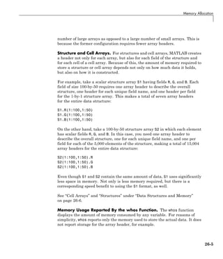
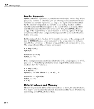
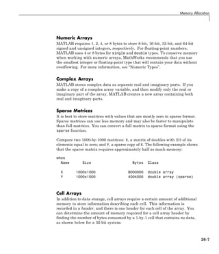
![26 Memory Usage
A = {[]}; % Empty cell array
whos A
Name Size Bytes Class Attributes
A 1x1 60 cell
In this case, MATLAB shows the number of bytes required for each header in
the cell array on a 32-bit system to be 60. This is the header size that is used
in all of the 32-bit examples in this section. For 64-bit systems, the header
size is assumed to be 112 bytes in this documentation. You can find the
correct header size on a 64-bit system using the method just shown for 32 bits.
To predict the size of an entire cell array, multiply the number you have just
derived for the header by the total number of cells in the array, and then
add to that the number of bytes required for the data you intend to store
in the array:
(header_size x number_of_cells) + data
So a 10-by-20 cell array that contains 400 bytes of data would require 22,800
bytes of memory on a 64-bit system:
(112 x 200) + 400 = 22800
Note While numeric arrays must be stored in contiguous memory, structures
and cell arrays do not.
Example 1 – Memory Allocation for a Cell Array. The following 4-by-1
cell array records the brand name, screen size, price, and on-sale status for
three laptop computers:
Laptops = {['SuperrrFast 89X', 'ReliablePlus G5', ...
'UCanA4dIt 140L6']; ...
[single(17), single(15.4), single(14.1)]; ...
[2499.99, 1199.99, 499.99]; ...
[true, true, false]};
On a 32-bit system, the cell array header alone requires 60 bytes per cell:
26-8](https://image.slidesharecdn.com/matlabprog-220902050722-ff974cdf/85/matlab_prog-pdf-836-320.jpg)
![Memory Allocation
4 cells * 60 bytes per cell = 240 bytes for the cell array
Calculate the memory required to contain the data in each of the four cells:
45 characters * 2 bytes per char = 90 bytes
3 doubles * 8 bytes per double = 24 bytes
3 singles * 4 bytes per single = 12 bytes
3 logicals * 1 byte per logical = 3 bytes
90 + 24 + 12 + 3 = 129 bytes for the data
Add the two, and then compare your result with the size returned by
MATLAB:
240 + 129 = 369 bytes total
whos Laptops
Name Size Bytes Class Attributes
Laptops 4x1 369 cell
Structures
S.A = [];
B = whos('S');
B.bytes - 60
ans =
64
Compute the memory needed for a structure array as follows:
32-bit systems: fields x ((60 x array elements) + 64) + data
64-bit systems: fields x ((112 x array elements) + 64) + data
On a 64-bit computer system, a 4-by-5 structure Clients with fields Address
and Phone uses 4,608 bytes just for the structure:
2 fields x ((112 x 20) + 64) = 2 x (2240 + 64) = 4608 bytes
To that sum, you must add the memory required to hold the data assigned to
each field. If you assign a 25-character string to Address and a 12-character
26-9](https://image.slidesharecdn.com/matlabprog-220902050722-ff974cdf/85/matlab_prog-pdf-837-320.jpg)
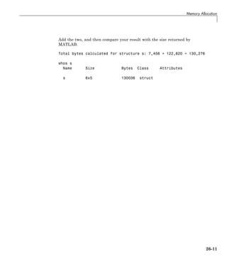
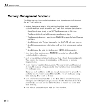
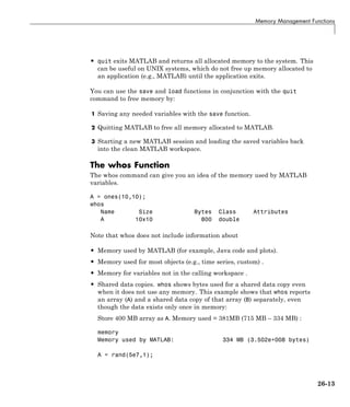
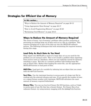
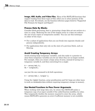
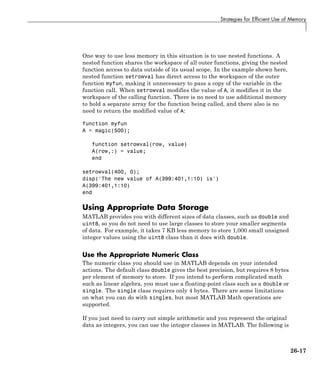
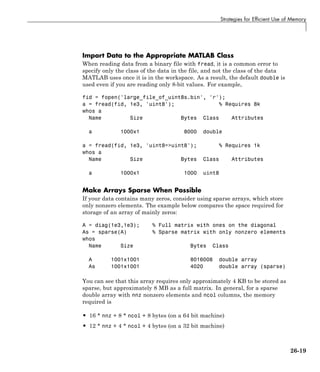
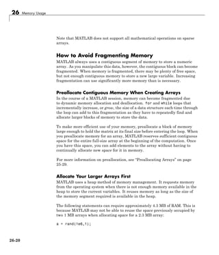
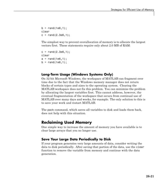
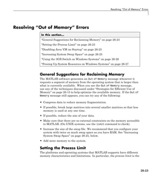
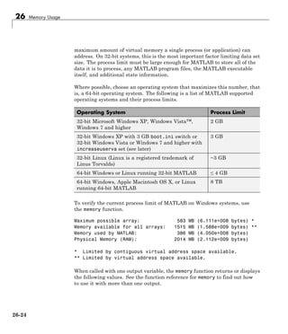
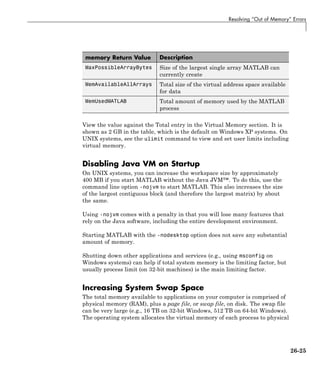
![26 Memory Usage
memory or to the swap file, depending on the needs of the system and other
processes.
Most systems allow you to control the size of your swap file. The steps
involved depend on the system you are running on.
Note There is no interface for directly controlling the swap space on
Macintosh OS X systems.
Windows Systems
Use the Windows Control Panel to change the size of the virtual memory
paging file on your system. For more information, refer to the Windows help.
Linux Systems
You can change your swap space by using the mkswap and swapon commands.
For more information on the above commands, type man followed by the
command name at the Linux prompt.
Using the 3GB Switch on Windows Systems
Microsoft Windows XP systems can allocate 3 GB (instead of the default 2
GB) to processes, if you set an appropriate switch in the boot.ini file of the
system. MathWorks recommends that you only do this with Windows XP SP2
systems or later. This gives an extra 1 GB of virtual memory to MATLAB, not
contiguous with the rest of the memory. This enables you to store more data,
but not larger arrays, as these are limited by contiguous space. This is mostly
beneficial if you have enough RAM (e.g., 3 or 4 GB) to use it.
After setting the switch, confirm the new value of the virtual memory after
restarting your computer and using the memory function.
[userview systemview] = memory;
systemview.VirtualAddressSpace
ans =
Available: 1.6727e+009 % Virtual memory available to MATLAB.
Total: 2.1474e+009 % Total virtual memory
26-26](https://image.slidesharecdn.com/matlabprog-220902050722-ff974cdf/85/matlab_prog-pdf-854-320.jpg)

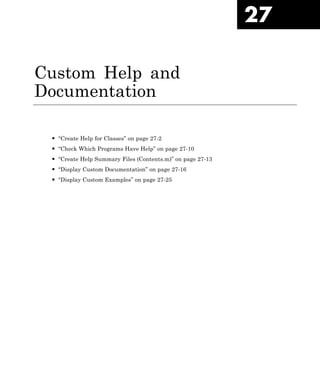
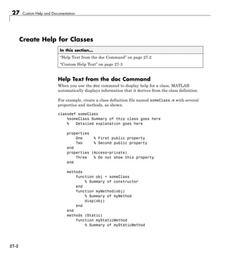
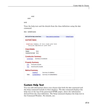
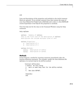
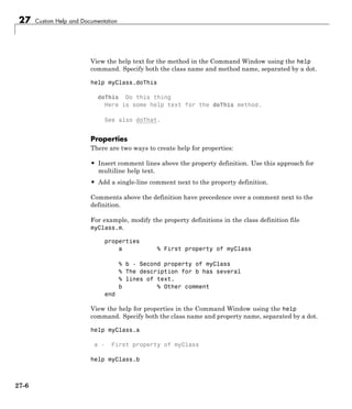
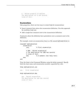
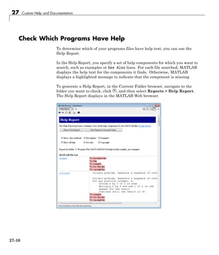
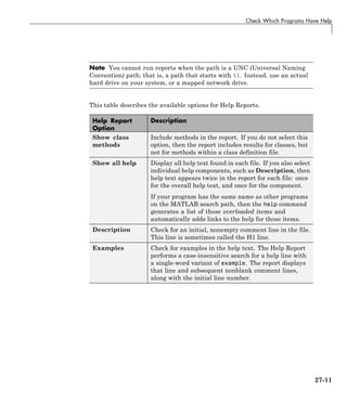
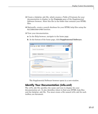
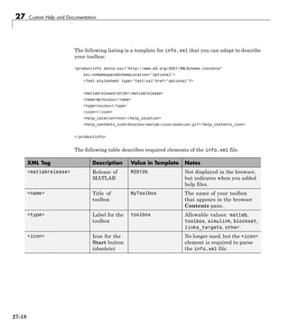
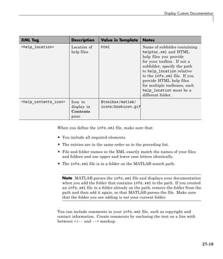
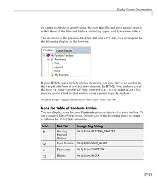
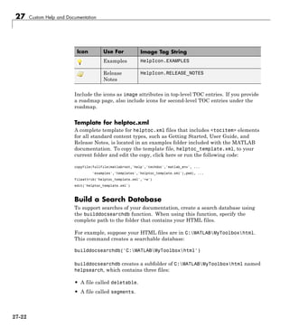
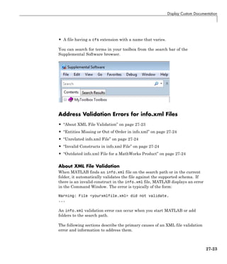
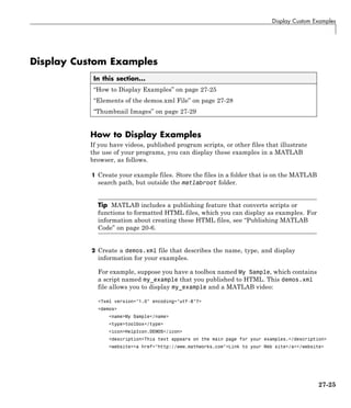
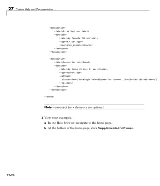
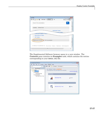
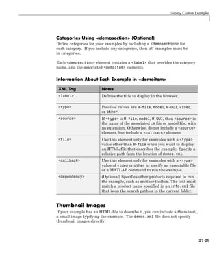
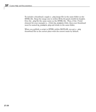
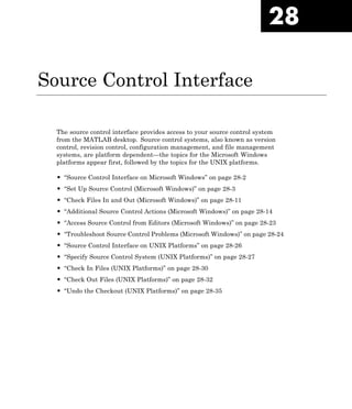
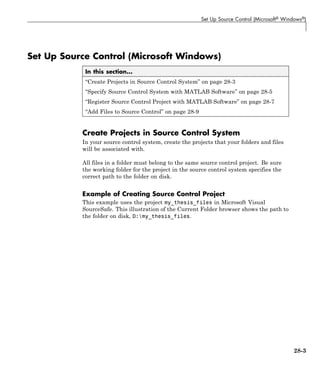
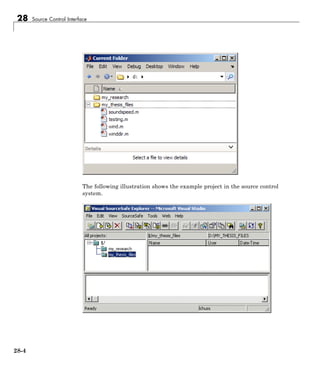
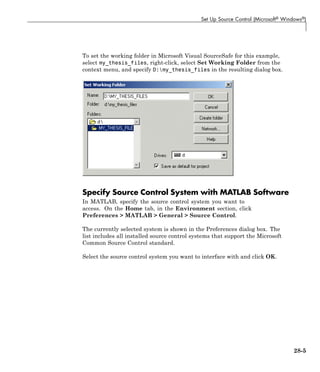
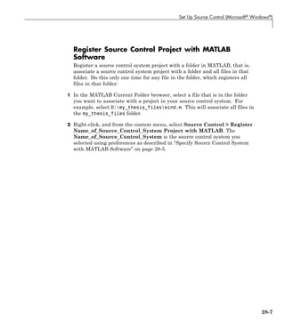
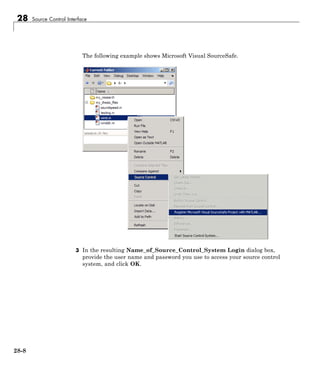
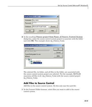
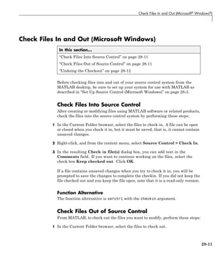
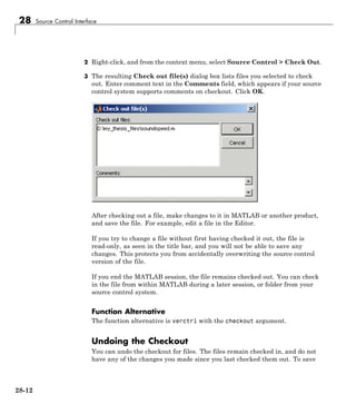
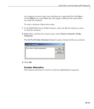

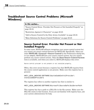
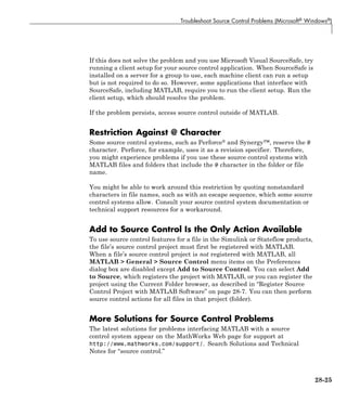

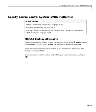
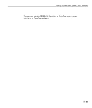
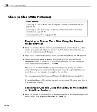
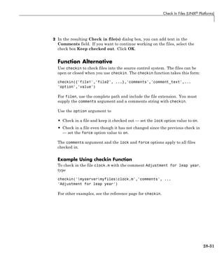
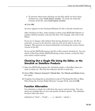
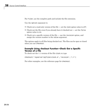
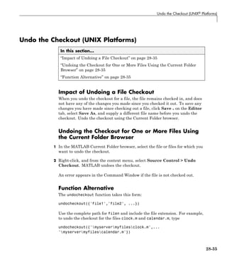

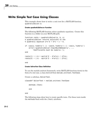
![Write Simple Test Case Using Classes
Create Test Method for Real Solutions
Create a test method, testRealSolution, to verify that quadraticSolver
returns the right value for real solutions. For example, the equation
x2
- 3x + 2 = 0 has real solutions x = 1 and x = 2. This method
calls quadraticSolver with the inputs of this equation. The solution,
expSolution, is [2,1].
Use the matlab.unittest.TestCase method, verifyEqual to compare the
output of the function, actSolution, to the desired output, expSolution. If
the qualification fails, the test continues execution.
function testRealSolution(testCase)
actSolution = quadraticSolver(1,-3,2);
expSolution = [2,1];
testCase.verifyEqual(actSolution,expSolution);
end
Add this function inside the methods (Test) block.
Create Test Method for Imaginary Solutions
Create a test to verify that quadraticSolver returns the right value for
imaginary solutions. For example, the equation x2
- 2x + 10 = 0 has
imaginary solutions x = -1 + 3i and x = -1 - 3i. Add this function,
testImaginarySolution, inside the methods (Test) block.
function testImaginarySolution(testCase)
actSolution = quadraticSolver(1,2,10);
expSolution = [-1+3i, -1-3i];
testCase.verifyEqual(actSolution,expSolution);
end
The order of the tests within the block does not matter.
Save Class Definition
The following is the complete SolverTest class definition. Save this file in a
folder on your MATLAB path.
classdef SolverTest < matlab.unittest.TestCase
29-3](https://image.slidesharecdn.com/matlabprog-220902050722-ff974cdf/85/matlab_prog-pdf-925-320.jpg)
![29 Unit Testing
% SolverTest tests solutions to the quadratic equation
% a*x^2 + b*x + c = 0
methods (Test)
function testRealSolution(testCase)
actSolution = quadraticSolver(1,-3,2);
expSolution = [2,1];
testCase.verifyEqual(actSolution,expSolution);
end
function testImaginarySolution(testCase)
actSolution = quadraticSolver(1,2,10);
expSolution = [-1+3i, -1-3i];
testCase.verifyEqual(actSolution,expSolution);
end
end
end
Run Tests in SolverTest Test Case
Run all the tests in the SolverTest class definition file.
testCase = SolverTest;
res = run(testCase)
Running SolverTest
..
Done SolverTest
__________
res =
1x2 TestResult array with properties:
Name
Passed
Failed
Incomplete
Duration
Totals:
2 Passed, 0 Failed, 0 Incomplete.
29-4](https://image.slidesharecdn.com/matlabprog-220902050722-ff974cdf/85/matlab_prog-pdf-926-320.jpg)
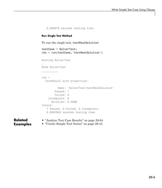
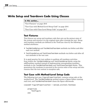
![Write Setup and Teardown Code Using Classes
methods(TestMethodSetup)
function createFigure(testCase)
%comment
testCase.TestFigure = figure;
end
end
methods(TestMethodTeardown)
function closeFigure(testCase)
close(testCase.TestFigure);
end
end
methods(Test)
function defaultCurrentPoint(testCase)
cp = get(testCase.TestFigure, 'CurrentPoint');
testCase.verifyEqual(cp, [0 0], ...
'Default current point is incorrect')
end
function defaultCurrentObject(testCase)
import matlab.unittest.constraints.IsEmpty;
co = get(testCase.TestFigure, 'CurrentObject');
testCase.verifyThat(co, IsEmpty, ...
'Default current object should be empty');
end
end
end
Test Case with Class-Level Setup Code
The following test case, BankAccountTest, contains setup code at the class
level.
29-7](https://image.slidesharecdn.com/matlabprog-220902050722-ff974cdf/85/matlab_prog-pdf-929-320.jpg)
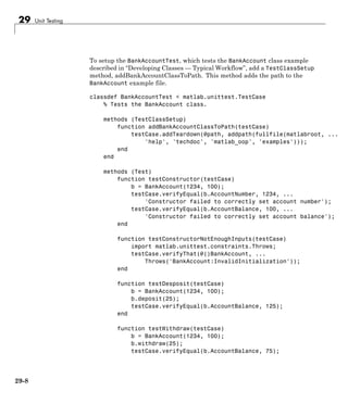
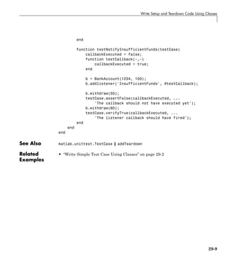
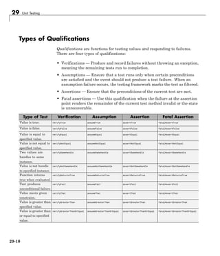
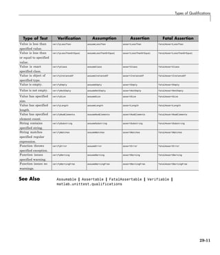
![29 Unit Testing
Write Tests Using Shared Fixtures
This example shows how to use shared fixtures when creating tests. You
can share test fixtures across test classes using the SharedTestFixtures
attribute of the TestCase class. To exemplify this attribute, create multiple
test classes in a subdirectory of your current working folder. The test methods
are shown only at a high level.
The two test classes used in this example test the DocPolynom class and the
BankAccount class. You can access both classes in MATLAB, but you must add
them to the MATLAB path. A path fixture adds the directory to the current
path, runs the tests, and removes the directory from the path. Since both
classes require the same addition to the path, the tests use a shared fixture.
Create a Test for the DocPolynom Class
Create a test file for the DocPolynom class. Create the shared fixture by
specifying the SharedTestFixtures attribute for the TestCase and passing in
a PathFixture.
DocPolynomTest Class Definition File
classdef (SharedTestFixtures={matlab.unittest.fixtures.PathFixture( ...
fullfile(matlabroot, 'help', 'techdoc', 'matlab_oop', 'examples'))}
DocPolynomTest < matlab.unittest.TestCase
% Tests the DocPolynom class.
properties
msgEqn = 'Equation under test: ';
end
methods (Test)
function testConstructor(testCase)
p = DocPolynom([1, 0, 1]);
testCase.verifyClass(p, ?DocPolynom);
end
function testAddition(testCase)
p1 = DocPolynom([1, 0, 1]);
p2 = DocPolynom([5, 2]);
29-12](https://image.slidesharecdn.com/matlabprog-220902050722-ff974cdf/85/matlab_prog-pdf-934-320.jpg)
![Write Tests Using Shared Fixtures
actual = p1 + p2;
expected = DocPolynom([1, 5, 3]);
msg = [testCase.msgEqn,...
'(x^2 + 1) + (5*x + 2) = x^2 + 5*x + 3'];
testCase.verifyEqual(actual, expected, msg);
end
function testMultiplication(testCase)
p1 = DocPolynom([1, 0, 3]);
p2 = DocPolynom([5, 2]);
actual = p1 * p2;
expected = DocPolynom([5, 2, 15, 6]);
msg = [testCase.msgEqn,...
'(x^2 + 3) * (5*x + 2) = 5*x^3 + 2*x^2 + 15*x + 6'];
testCase.verifyEqual(actual, expected, msg);
end
end
end
Create a Test for the BankAccount Class
Create a test file for the BankAccount class. Create the shared fixture by
specifying the SharedTestFixtures attribute for the TestCase and passing in
a PathFixture.
BankAccountTest Class Definition File
classdef (SharedTestFixtures={matlab.unittest.fixtures.PathFixture( ...
fullfile(matlabroot, 'help', 'techdoc', 'matlab_oop', ...
'examples'))}) BankAccountTest < matlab.unittest.TestCase
% Tests the BankAccount class.
methods (Test)
function testConstructor(testCase)
b = BankAccount(1234, 100);
29-13](https://image.slidesharecdn.com/matlabprog-220902050722-ff974cdf/85/matlab_prog-pdf-935-320.jpg)
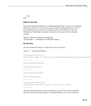
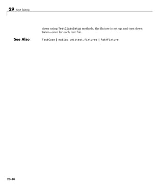
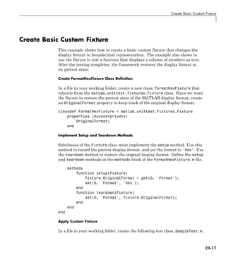
![29 Unit Testing
classdef SampleTest < matlab.unittest.TestCase
methods (Test)
function test1(testCase)
testCase.applyFixture(FormatHexFixture);
actStr = getColumnForDisplay([1;2;3], 'Small Integers');
expStr = ['Small Integers '
'3ff0000000000000'
'4000000000000000'
'4008000000000000'];
testCase.verifyEqual(actStr, expStr);
end
end
end
function str = getColumnForDisplay(values, title)
elements = cell(numel(values)+1, 1);
elements{1} = title;
for idx = 1:numel(values)
elements{idx+1} = displayNumber(values(idx));
end
str = char(elements);
end
function str = displayNumber(n)
str = strtrim(evalc('disp(n);'));
end
This test applies the custom fixture and verifies that the displayed column of
hexadecimal representation is as expected.
At the command prompt, run the test.
run(SampleTest);
Running SampleTest
.
Done SampleTest
__________
See Also matlab.unittest.fixtures.Fixture
29-18](https://image.slidesharecdn.com/matlabprog-220902050722-ff974cdf/85/matlab_prog-pdf-940-320.jpg)
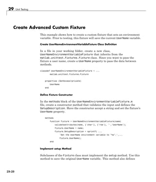
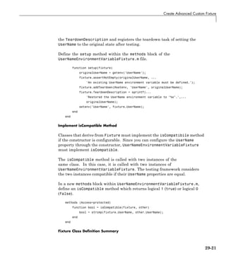
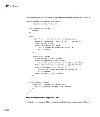
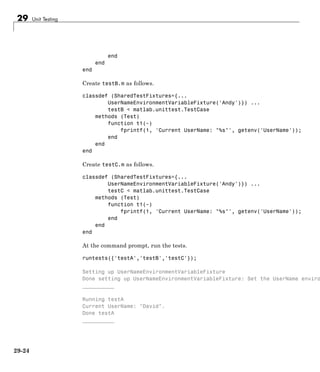
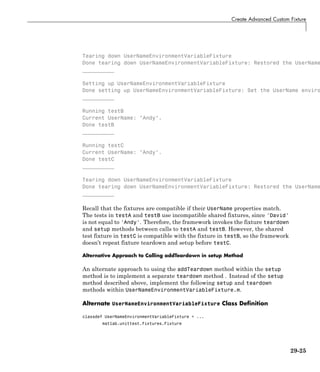
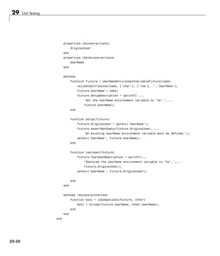
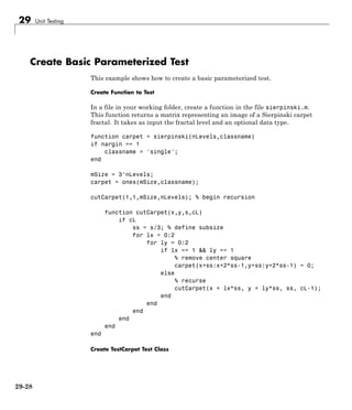
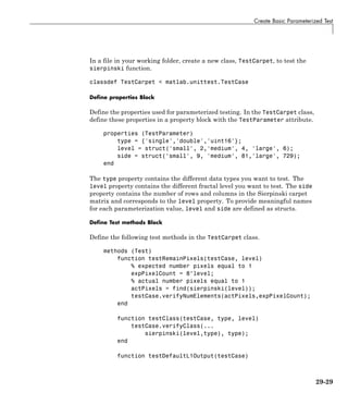
![29 Unit Testing
exp = single([1 1 1; 1 0 1; 1 1 1]);
testCase.verifyEqual(sierpinski(1), exp);
end
end
The testRemainPixes method tests the output of the sierpinski function
by verifying that the number of nonzero pixels is the same as expected
for a particular level. This method uses the level property and, therefore,
results in three test elements—one for each value in level. The testClass
method tests the class of the output from the sierpinski function with
each combination of the type and level properties. This approach results
in nine test elements. The testDefaultL1Output test method does not use
a TestParameter property and, therefore, is not parameterized. This test
method verifies that the level 1 matrix contains the expected values. Since
the test method is not parameterized, it results in a one test element.
In the test methods above, you did not define the ParameterCombination
attribute of the Test methods block. This attribute is, by default,
'exhaustive'. The test framework invokes a given test method once for
every combination of the test parameters.
Define Test methods Block with ParameterCombination Attribute
Define the following test methods in the TestCarpet class to ensure that
the matrix output by the sierpinski function has the correct number of
elements. Set the ParameterCombination attribute to 'sequential'.
methods (Test, ParameterCombination='sequential')
function testNumel(testCase, level, side)
import matlab.unittest.constraints.HasElementCount;
testCase.verifyThat(sierpinski(level),...
HasElementCount(side^2));
end
end
end
Test methods with the ParameterCombination attribute set to 'sequential'
are invoked once for each corresponding value of the parameter. The
properties, level and side, must have the same number of values. Since
29-30](https://image.slidesharecdn.com/matlabprog-220902050722-ff974cdf/85/matlab_prog-pdf-952-320.jpg)
![Create Basic Parameterized Test
these properties each have three values, the testNumel method is invoked
three times.
TestCarpet Class Definition Summary
The complete contents of TestCarpet.m follows.
classdef TestCarpet < matlab.unittest.TestCase
properties (TestParameter)
type = {'single','double','uint16'};
level = struct('small', 2,'medium', 4, 'large', 6);
side = struct('small', 9, 'medium', 81,'large', 729);
end
methods (Test)
function testRemainPixels(testCase, level)
% expected number pixels equal to 1
expPixelCount = 8^level;
% actual number pixels equal to 1
actPixels = find(sierpinski(level));
testCase.verifyNumElements(actPixels,expPixelCount);
end
function testClass(testCase, type, level)
testCase.verifyClass(...
sierpinski(level,type), type);
end
function testDefaultL1Output(testCase)
exp = single([1 1 1; 1 0 1; 1 1 1]);
testCase.verifyEqual(sierpinski(1), exp);
end
end
methods (Test, ParameterCombination='sequential')
function testNumel(testCase, level, side)
import matlab.unittest.constraints.HasElementCount;
testCase.verifyThat(sierpinski(level),...
HasElementCount(side^2));
29-31](https://image.slidesharecdn.com/matlabprog-220902050722-ff974cdf/85/matlab_prog-pdf-953-320.jpg)
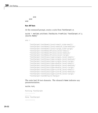
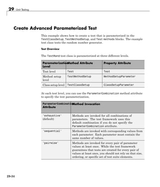
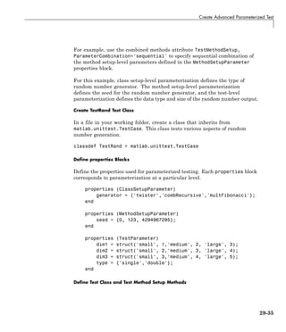
![29 Unit Testing
Define the setup methods at the test class and test method level. These
methods register the initial random number generator state. After the
framework runs the tests, the methods restore the original state. The
ClassSetup method defines the type of random number generator, and the
TestMethodSetup seeds the generator.
methods (TestClassSetup)
function ClassSetup(testCase, generator)
orig = rng;
testCase.addTeardown(@rng, orig);
rng(0, generator);
end
end
methods (TestMethodSetup)
function MethodSetup(testCase, seed)
orig = rng;
testCase.addTeardown(@rng, orig);
rng(seed);
end
end
Define Sequential Parameterized Test Methods
Define a methods block with the Test and
ParameterCombination='sequential' attributes. The test framework
invokes these methods once for each corresponding property value.
methods (Test, ParameterCombination='sequential')
function testSize(testCase,dim1,dim2,dim3)
testCase.verifySize(rand(dim1,dim2,dim3),[dim1 dim2 dim3]);
end
end
The method tests the size of the output for each corresponding parameter
in dim1, dim2, and dim3. For example, to test all the 'medium' values
use: testCase.verifySize(rand(2,3,4),[2 3 4]);. For a given
TestClassSetup and TestMethodSetup parameterization, the framework
calls the testSize method three times—once each for the 'small', 'medium',
and 'large' values.
29-36](https://image.slidesharecdn.com/matlabprog-220902050722-ff974cdf/85/matlab_prog-pdf-958-320.jpg)
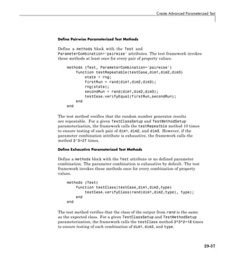
![29 Unit Testing
TestRand Class Definition Summary
classdef TestRand < matlab.unittest.TestCase
properties (ClassSetupParameter)
generator = {'twister','combRecursive','multFibonacci'};
end
properties (MethodSetupParameter)
seed = {0, 123, 4294967295};
end
properties (TestParameter)
dim1 = struct('small', 1,'medium', 2, 'large', 3);
dim2 = struct('small', 2,'medium', 3, 'large', 4);
dim3 = struct('small', 3,'medium', 4, 'large', 5);
type = {'single','double'};
end
methods (TestClassSetup)
function ClassSetup(testCase, generator)
orig = rng;
testCase.addTeardown(@rng, orig);
rng(0, generator);
end
end
methods (TestMethodSetup)
function MethodSetup(testCase, seed)
orig = rng;
testCase.addTeardown(@rng, orig);
rng(seed);
end
end
methods (Test, ParameterCombination='sequential')
function testSize(testCase,dim1,dim2,dim3)
testCase.verifySize(rand(dim1,dim2,dim3),[dim1 dim2 dim3]);
end
end
29-38](https://image.slidesharecdn.com/matlabprog-220902050722-ff974cdf/85/matlab_prog-pdf-960-320.jpg)
![29 Unit Testing
ans =
TestRand[generator=twister]/[seed=value1]testClass(dim1=small,dim2=small,ty
The name of each element is constructed from the combination of the
following:
• Test class: TestRand
• Class setup property and property name: [generator=twister]
• Method setup property and property name: [seed=value1]
• Test method name: testClass
• Test method properties and property names:
(dim1=small,dim2=small,type=single)
The name for the seed property isn’t particularly meaningful (value1). The
testing framework provided this name because the seed property values are
numbers. For a more meaningful name, define the seed property as a struct
with more descriptive field names.
Run Suite from Class Using Selector
At the command prompt, create a selector to select test elements that test the
'twister' generator for 'single' precision. Omit test elements that use
properties with the 'large' name.
import matlab.unittest.selectors.HasParameter
s = HasParameter('Property','generator', 'Name','twister') & ...
HasParameter('Property','type', 'Name','single') & ...
~HasParameter('Name','large');
suite2 = matlab.unittest.TestSuite.fromClass(?TestRand,s)
suite2 =
1x12 Test array with properties:
Name
Parameterization
SharedTestFixtures
29-40](https://image.slidesharecdn.com/matlabprog-220902050722-ff974cdf/85/matlab_prog-pdf-962-320.jpg)
![Create Advanced Parameterized Test
If you first generate the full suite, construct the same test suite as above
using the selectIf method.
suite = matlab.unittest.TestSuite.fromClass(?TestRand);
suite2 = selectIf(suite,s);
Run the test suite.
suite2.run;
Running TestRand
..........
..
Done TestRand
__________
Run Suite from Method Using Selector
At the command prompt, create a selector that omits test elements that use
properties with the 'large' or 'medium' name. Limit results to test elements
from the testRepeatable method.
import matlab.unittest.selectors.HasParameter
s = ~(HasParameter('Name','large') | HasParameter('Name','medium'));
suite3 = matlab.unittest.TestSuite.fromMethod(?TestRand,'testRepeatable',s);
{suite3.Name}'
ans =
'TestRand[generator=twister]/[seed=value1]testRepeatable(dim1=small,dim2=small,dim3=small)'
'TestRand[generator=twister]/[seed=value2]testRepeatable(dim1=small,dim2=small,dim3=small)'
'TestRand[generator=twister]/[seed=value3]testRepeatable(dim1=small,dim2=small,dim3=small)'
'TestRand[generator=combRecursive]/[seed=value1]testRepeatable(dim1=small,dim2=small,dim3=sm
'TestRand[generator=combRecursive]/[seed=value2]testRepeatable(dim1=small,dim2=small,dim3=sm
'TestRand[generator=combRecursive]/[seed=value3]testRepeatable(dim1=small,dim2=small,dim3=sm
'TestRand[generator=multFibonacci]/[seed=value1]testRepeatable(dim1=small,dim2=small,dim3=sm
'TestRand[generator=multFibonacci]/[seed=value2]testRepeatable(dim1=small,dim2=small,dim3=sm
'TestRand[generator=multFibonacci]/[seed=value3]testRepeatable(dim1=small,dim2=small,dim3=sm
Run the test suite.
29-41](https://image.slidesharecdn.com/matlabprog-220902050722-ff974cdf/85/matlab_prog-pdf-963-320.jpg)
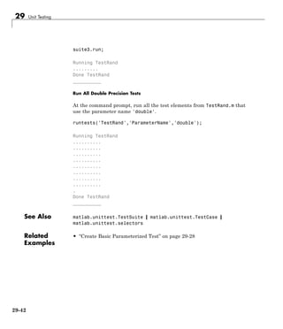
![Create Simple Test Suites
Create Simple Test Suites
This example shows how to combine tests into test suites, using
the SolverTest test case. Use the static from* methods in the
matlab.unittest.TestSuite class to create suites for combinations of your tests,
whether they are organized in packages and classes or files and folders, or
both.
Create Quadratic Solver Function
Create the following function that solves roots of the quadratic equation in a
file, quadraticSolver.m, in your working folder.
function roots = quadraticSolver(a, b, c)
% quadraticSolver returns solutions to the
% quadratic equation a*x^2 + b*x + c = 0.
if ~isa(a,'numeric') || ~isa(b,'numeric') || ~isa(c,'numeric')
error('quadraticSolver:InputMustBeNumeric', ...
'Coefficients must be numeric.');
end
roots(1) = (-b + sqrt(b^2 - 4*a*c)) / (2*a);
roots(2) = (-b - sqrt(b^2 - 4*a*c)) / (2*a);
end
Create Test for Quadratic Solver Function
Create the following test class in a file, SolverTest.m, in your working folder.
classdef SolverTest < matlab.unittest.TestCase
% SolverTest tests solutions to the quadratic equation
% a*x^2 + b*x + c = 0
methods (Test)
function testRealSolution(testCase)
actSolution = quadraticSolver(1,-3,2);
expSolution = [2,1];
testCase.verifyEqual(actSolution,expSolution);
29-43](https://image.slidesharecdn.com/matlabprog-220902050722-ff974cdf/85/matlab_prog-pdf-965-320.jpg)
![29 Unit Testing
end
function testImaginarySolution(testCase)
actSolution = quadraticSolver(1,2,10);
expSolution = [-1+3i, -1-3i];
testCase.verifyEqual(actSolution,expSolution);
end
end
end
Import TestSuite Class
At the command prompt, add the matlab.unittest.TestSuite class to the
current import list.
import matlab.unittest.TestSuite;
Make sure the SolverTest class definition file is on your MATLAB path.
Create Suite from SolverTest Class
The fromClass method creates a suite from all Test methods in the
SolverTest class.
suiteClass = TestSuite.fromClass(?SolverTest);
result = run(suiteClass);
Create Suite from SolverTest Class Definition File
The fromFile method creates a suite using the name of the file to identify
the class.
suiteFile = TestSuite.fromFile('SolverTest.m');
result = run(suiteFile);
Create Suite from All Test Case Files in Current Folder
The fromFolder method creates a suite from all test case files in the specified
folder. For example, the following files are in the current folder:
• BankAccountTest.m
29-44](https://image.slidesharecdn.com/matlabprog-220902050722-ff974cdf/85/matlab_prog-pdf-966-320.jpg)
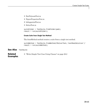
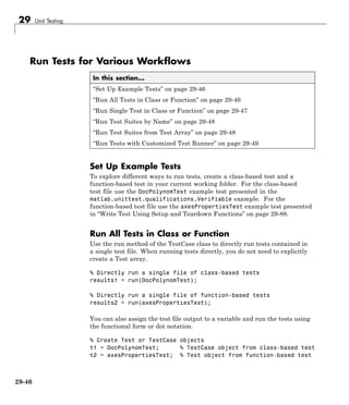
![29 Unit Testing
results2 = t2(2).run; % or results2 = run(t2(2));
Run Test Suites by Name
You can run a group, or suite, of tests together. To run the test suite using
runtests, the suite is defined as a cell array of strings representing a test
file, a test class, a package that contains tests or a folder that contains tests.
suite = {'axesPropertiesTest','DocPolynomTest'};
runtests(suite);
Run all tests in the current folder using the pwd as input to the runtests
function.
runtests(pwd);
Alternatively, you can explicitly create Test arrays and use the run method
to run them.
Run Test Suites from Test Array
You can explicitly create Test arrays and use the run method in the TestSuite
class to run them. Using this approach, you explicitly define TestSuite objects
and, therefore, can examine the contents. The runtests function does not
return the TestSuite object.
import matlab.unittest.TestSuite;
s1 = TestSuite.fromClass(?DocPolynomTest);
s2 = TestSuite.fromFile('axesPropertiesTest.m');
% generate test suite and then run
fullSuite = [s1 s2];
result = run(fullSuite);
Since the suite is explicitly defined, it is easy for you to perform further
analysis on the suite, such as rerunning failed tests.
failedTests = fullSuite([result.Failed]);
result2 = run(failedTests);
29-48](https://image.slidesharecdn.com/matlabprog-220902050722-ff974cdf/85/matlab_prog-pdf-970-320.jpg)
![Run Tests for Various Workflows
Run Tests with Customized Test Runner
You can specialize the test running by defining a custom test runner and
adding plugins. The run method of the TestRunner class operates on a
TestSuite object.
import matlab.unittest.TestRunner;
import matlab.unittest.TestSuite;
import matlab.unittest.plugins.TestSuiteProgressPlugin;
% Generate TestSuite.
s1 = TestSuite.fromClass(?DocPolynomTest);
s2 = TestSuite.fromFile('axesPropertiesTest.m');
suite = [s1 s2];
% Create silent test runner.
runner = TestRunner.withNoPlugins;
% Add plugin to display test progress.
runner.addPlugin(TestSuiteProgressPlugin);
% Run tests using customized runner.
result = run(runner,[s1 s2]);
See Also runtests | matlab.unittest.TestCase.run |
matlab.unittest.TestSuite.run | matlab.unittest.TestRunner.run
29-49](https://image.slidesharecdn.com/matlabprog-220902050722-ff974cdf/85/matlab_prog-pdf-971-320.jpg)
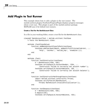
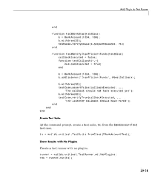
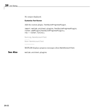
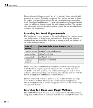
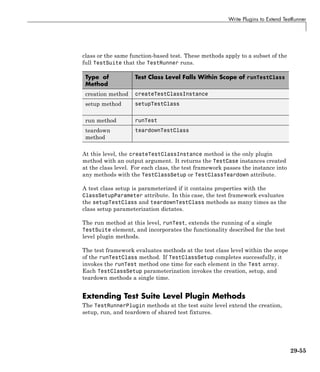
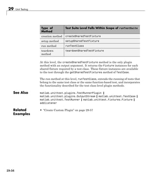
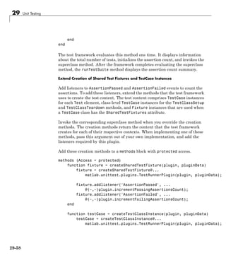
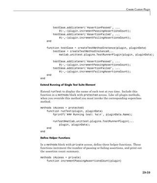
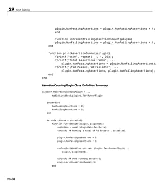
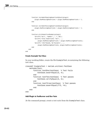
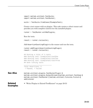
![29 Unit Testing
Analyze Test Case Results
This example shows how to analyze the information returned by a test runner
created from the SolverTest test case.
Create Quadratic Solver Function
Create the following function that solves roots of the quadratic equation in a
file, quadraticSolver.m, in your working folder.
function roots = quadraticSolver(a, b, c)
% quadraticSolver returns solutions to the
% quadratic equation a*x^2 + b*x + c = 0.
if ~isa(a,'numeric') || ~isa(b,'numeric') || ~isa(c,'numeric')
error('quadraticSolver:InputMustBeNumeric', ...
'Coefficients must be numeric.');
end
roots(1) = (-b + sqrt(b^2 - 4*a*c)) / (2*a);
roots(2) = (-b - sqrt(b^2 - 4*a*c)) / (2*a);
end
Create Test for Quadratic Solver Function
Create the following test class in a file, SolverTest.m, in your working folder.
classdef SolverTest < matlab.unittest.TestCase
% SolverTest tests solutions to the quadratic equation
% a*x^2 + b*x + c = 0
methods (Test)
function testRealSolution(testCase)
actSolution = quadraticSolver(1,-3,2);
expSolution = [2,1];
testCase.verifyEqual(actSolution,expSolution);
end
function testImaginarySolution(testCase)
actSolution = quadraticSolver(1,2,10);
29-64](https://image.slidesharecdn.com/matlabprog-220902050722-ff974cdf/85/matlab_prog-pdf-986-320.jpg)
![Analyze Test Case Results
expSolution = [-1+3i, -1-3i];
testCase.verifyEqual(actSolution,expSolution);
end
end
end
Run SolverTest Test Case
Create a test suite, quadTests.
quadTests = matlab.unittest.TestSuite.fromClass(?SolverTest);
result = run(quadTests);
Running SolverTest
..
Done SolverTest
__________
All tests passed.
Explore Output Argument, result
The output argument, result, is a matlab.unittest.TestResult object. It
contains information of the two tests in SolverTest.
whos result
Name Size Bytes Class
result 1x2 248 matlab.unittest.TestResult
Display Information for One Test
To see the information for one value, type:
result(1)
ans =
TestResult with properties:
29-65](https://image.slidesharecdn.com/matlabprog-220902050722-ff974cdf/85/matlab_prog-pdf-987-320.jpg)
![Analyze Failed Test Results
Analyze Failed Test Results
This example shows how to identify and rerun failed tests.
Create an Incorrect Test Method
Using the SolverTest test case, add a method, testBadRealSolution. This
test, based on testRealSolution, calls the quadraticSolver function with
inputs 1,3,2, but tests the results against an incorrect solution, [2,1].
function testBadRealSolution(testCase)
actSolution = quadraticSolver(1,3,2);
expSolution = [2,1];
testCase.verifyEqual(actSolution,expSolution);
end
Run New Test Suite
Save the updated SolverTest class definition and rerun the tests.
quadTests = matlab.unittest.TestSuite.fromClass(?SolverTest);
result1 = run(quadTests);
Running SolverTest
.
===========================================================================
Verification failed in SolverTest/testBadRealSolution.
---------------------
Framework Diagnostic:
---------------------
verifyEqual failed.
--> NumericComparator failed.
--> The values are not equal using "isequaln".
Actual Value:
-1 -2
Expected Value:
2 1
------------------
29-67](https://image.slidesharecdn.com/matlabprog-220902050722-ff974cdf/85/matlab_prog-pdf-989-320.jpg)
![29 Unit Testing
Stack Information:
------------------
In C:Program FilesMATLABR2013atoolboxmatlabtestframework+matlab
In c:workSolverTest.m (SolverTest.testBadRealSolution) at 15
===========================================================================
....
Done SolverTest
__________
Failure Summary:
Name Failed Incomplete Reason(s)
=======================================================================
SolverTest/testBadRealSolution X Failed by verifica
>>
Analyze Results
The output tells you SolverTest/testBadRealSolution failed. From the
Framework Diagnostic you see the following:
Actual Value:
-1 -2
Expected Value:
2 1
At this point, you must decide if the error is in quadraticSolver or in your
value for expSolution.
Correct Error
Edit the value of expSolution in testBadRealSolution:
expSolution = [-1 -2];
Rerun Tests
Save SolverTest and rerun only the failed tests.
failedTests = quadTests([result1.Failed]);
29-68](https://image.slidesharecdn.com/matlabprog-220902050722-ff974cdf/85/matlab_prog-pdf-990-320.jpg)
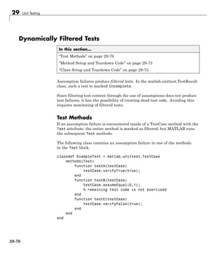
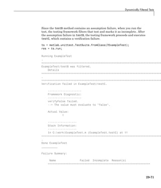
![29 Unit Testing
ExampleTest/testB X Filtered by assumption.
----------------------------------------------------------------
ExampleTest/testC X Failed by verification.
If you examine the TestResult, you notice that there is a passed test, a failed
test, and a test that did not complete due to an assumption failure.
res
res =
1x3 TestResult array with properties:
Name
Passed
Failed
Incomplete
Duration
Totals:
1 Passed, 1 Failed, 1 Incomplete.
0.059433 seconds testing time.
The testing framework keeps track of incomplete tests so that you can monitor
filtered tests for nonexercised test code. You can see information about these
tests within the TestResult object.
res([res.Incomplete])
ans =
TestResult with properties:
Name: 'ExampleTest/testB'
Passed: 0
Failed: 0
Incomplete: 1
Duration: 0.0400
Totals:
0 Passed, 0 Failed, 1 Incomplete.
29-72](https://image.slidesharecdn.com/matlabprog-220902050722-ff974cdf/85/matlab_prog-pdf-994-320.jpg)
![Dynamically Filtered Tests
0.040017 seconds testing time.
To create a modified test suite from only the filtered tests, select incomplete
tests from the original test suite.
tsFiltered = ts([res.Incomplete])
tsFiltered =
Test with properties:
Name: 'ExampleTest/testB'
Parameterization: []
SharedTestFixtures: []
Method Setup and Teardown Code
If an assumption failure is encountered inside a TestCase method with
the TestMethodSetup attribute, MATLAB filters the method which was
to be run for that instance. If a test uses assumptions from within the
TestMethodSetup block, consider instead using the assumptions in the
TestClassSetup block, which likewise filters all Test methods in the class
but is less verbose and more efficient.
One of the methods in the following TestMethodSetup block within
ExampleTest.m contains an assumption failure.
methods(TestMethodSetup)
function setupMethod1(testCase)
testCase.assumeEqual(1,0);
% remaining test code is not exercised
end
function setupMethod2(testCase)
disp('* Running setupMethod2 *')
testCase.assertEqual(1,1);
end
end
Updated ExampleTest Class Definition
classdef ExampleTest < matlab.unittest.TestCase
methods(TestMethodSetup)
29-73](https://image.slidesharecdn.com/matlabprog-220902050722-ff974cdf/85/matlab_prog-pdf-995-320.jpg)
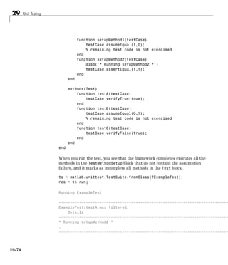
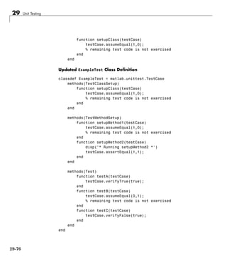
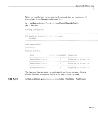
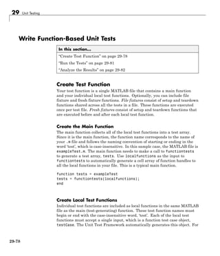
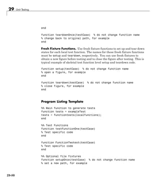
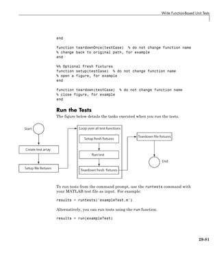
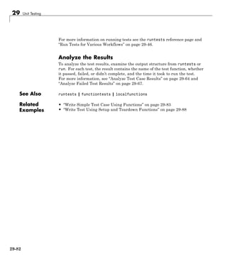
![29 Unit Testing
Create Test Function for Real Solutions
Create a test function, testRealSolution, to verify that quadraticSolver
returns the correct value for real solutions. For example, the equation x2
- 3x + 2 = 0 has real solutions x = 1 and x = 2. This function calls
quadraticSolver with the inputs of this equation. The expected solution,
expSolution, is [2,1].
Use the qualification function, verifyEqual, to compare the output of
the function, actSolution, to the desired output, expSolution. If the
qualification fails, the framework continues executing the test. Typically,
when using verifyEqual on floating point values, you specify a tolerance for
the comparison. For more information, see matlab.unittest.constraints.
Add this function to the solverTest.m file.
function testRealSolution(testCase)
actSolution = quadraticSolver(1,-3,2);
expSolution = [2,1];
verifyEqual(testCase,actSolution,expSolution);
end
Create Test Function for Imaginary Solutions
Create a test to verify that quadraticSolver returns the right value for
imaginary solutions. For example, the equation x2
- 2x + 10 = 0 has
imaginary solutions x = -1 + 3i and x = -1 - 3i. Typically, when
using verifyEqual on floating point values, you specify a tolerance for the
comparison. For more information, see matlab.unittest.constraints.
Add this function, testImaginarySolution, to the solverTest.m file.
function testImaginarySolution(testCase)
actSolution = quadraticSolver(1,2,10);
expSolution = [-1+3i, -1-3i];
verifyEqual(testCase,actSolution,expSolution);
end
The order of the tests within the solverTest.m file does not matter because
they are fully independent test cases.
29-84](https://image.slidesharecdn.com/matlabprog-220902050722-ff974cdf/85/matlab_prog-pdf-1006-320.jpg)
![Write Simple Test Case Using Functions
Save solverTest Function
The following is the complete solverTest.m test file. Save this file in a folder
on your MATLAB path.
function tests = solverTest
tests = functiontests(localfunctions);
end
function testRealSolution(testCase)
actSolution = quadraticSolver(1,-3,2);
expSolution = [2,1];
verifyEqual(testCase,actSolution,expSolution);
end
function testImaginarySolution(testCase)
actSolution = quadraticSolver(1,2,10);
expSolution = [-1+3i, -1-3i];
verifyEqual(testCase,actSolution,expSolution);
end
Run Tests in solverTest Function
Run the tests.
results = runtests('solverTest.m')
Running solverTest
..
Done solverTest
__________
results =
1x2 TestResult array with properties:
Name
Passed
Failed
29-85](https://image.slidesharecdn.com/matlabprog-220902050722-ff974cdf/85/matlab_prog-pdf-1007-320.jpg)
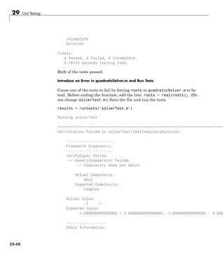
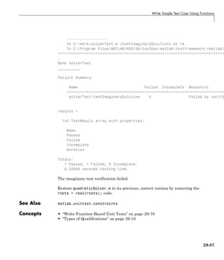
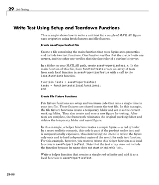
![Write Test Using Setup and Teardown Functions
function f = createFigure
f = figure;
ax = axes('Parent', f);
cylinder(ax,10);
h = findobj(ax,'Type','surface');
set(h,'FaceColor',[1 0 0]);
end
You must name the setup and teardown functions of a file test fixture
setupOnce and teardownOnce, respectively. These functions take a single
input argument, testCase, into which the test framework automatically
passes a function test case object. This test case object contains a TestData
structure that allows data to pass between setup, test, and teardown
functions. In this example, the TestData structure uses assigned fields to
store the original path, the temporary folder name, and the figure file name.
Create the setup and teardown functions as a local functions to
axesPropertiesTest.
function setupOnce(testCase)
% create and change to temporary folder
testCase.TestData.origPath = pwd;
testCase.TestData.tmpFolder = ['tmpFolder' datestr(now,30)];
mkdir(testCase.TestData.tmpFolder)
cd(testCase.TestData.tmpFolder)
% create and save a figure
testCase.TestData.figName = 'tmpFig.fig';
aFig = createFigure;
saveas(aFig,testCase.TestData.figName,'fig')
close(aFig)
end
function teardownOnce(testCase)
delete(testCase.TestData.figName);
cd(testCase.TestData.origPath);
rmdir(testCase.TestData.tmpFolder);
end
Create Fresh Fixture Functions
29-89](https://image.slidesharecdn.com/matlabprog-220902050722-ff974cdf/85/matlab_prog-pdf-1011-320.jpg)
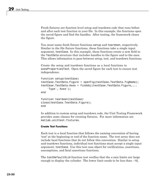
![Write Test Using Setup and Teardown Functions
and the upper limit needs to be greater than 10. These values come from
the figure generated in the helper function — a cylinder with a 10 unit
radius centered on the origin. This test function opens the figure created
and saved in the setupOnce function, queries the axes limit, and verifies
the limits are correct. The qualification functions, verifyLessThanOrEqual
and verifyGreaterThanOrEqual, takes the test case, the actual value, the
expected value, and optional diagnostic information to display in the case of
failure as inputs.
Create the testDefaultXLim function as local function to
axesPropertiesTest.
function testDefaultXLim(testCase)
xlim = get(testCase.TestData.Axes, 'XLim');
verifyLessThanOrEqual(testCase, xlim(1), -10,...
'Minimum x-limit was not small enough');
verifyGreaterThanOrEqual(testCase, xlim(2), 10,...
'Maximum x-limit was not big enough');
end
The surfaceColorTest function accesses the figure that you created and
saved in the setupOnce function. surfaceColorTest queries the face color of
the cylinder and verifies that it is red. The color red has an RGB value of [1 0
0]. The qualification function, verifyEqual, takes as inputs the test case,
the actual value, the expected value, and optional diagnostic information
to display in the case of failure. Typically when using verifyEqual on
floating point-values, you specify a tolerance for the comparison. For more
information, see matlab.unittest.constraints.
Create the surfaceColorTest function as local function to
axesPropertiesTest.
function surfaceColorTest(testCase)
h = findobj(testCase.TestData.Axes,'Type','surface');
co = get(h,'FaceColor');
verifyEqual(testCase, co, [1 0 0],'FaceColor is incorrect')
end
Now the axesPropertiesTest.m file is complete with a main function, file
fixture functions, fresh fixture functions, and two local test functions. You are
ready to run the tests.
29-91](https://image.slidesharecdn.com/matlabprog-220902050722-ff974cdf/85/matlab_prog-pdf-1013-320.jpg)
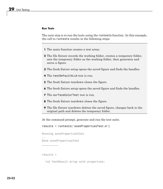
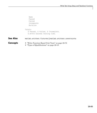

The document provides an overview of MATLAB programming fundamentals, including language syntax basics, variable creation, array vs. matrix operations, and command usage. It also details technical support contact information, copyright, trademarks, and patent protections for MATLAB software as of its 2014 release. Additional content includes a detailed table of contents outlining various programming concepts and operations available in MATLAB.