SOFTWARE TESTING
Yogesh Singh
CAMBRIDGE UNIVERSITY PRESS
Cambridge, New York, Melbourne, Madrid, Cape Town,
Singapore, São Paulo, Delhi, Tokyo, Mexico City
Cambridge University Press
4381/4, Ansari Road, Daryaganj, Delhi 110002, India
Published in the United States of America by Cambridge University Press, New York
www.cambridge.org
Information on this title: www.cambridge.org/9781107012967
© Yogesh Singh 2012
This publication is in copyright. Subject to statutory exception
and to the provisions of relevant collective licensing agreements,
no reproduction of any part may take place without the written
permission of Cambridge University Press.
First published 2012
Printed in India at...........
A catalogue record for this publication is available from the British Library
Library of Congress Cataloguing in Publication data
Singh, Yogesh, 1966-
Software testing / Yogesh Singh.
p. cm.
Includes bibliographical references.
Summary: “Discusses the concept of Software Testing with real-life case studies and solved
examples”-- Provided by publisher.
ISBN 978-1-107-01296-7 (hardback)
1. Computer software--Testing. 2. Computer software--Quality control. I. Title
QA76.76.T48S56 2011
005.1'4--dc22 2011012053
ISBN 978-1-107-01296-7 Hardback
Cambridge University Press has no responsibility for the persistence or
accuracy of URLs for external or third-party internet websites referred to in
this publication, and does not guarantee that any content on such websites is,
or will remain, accurate or appropriate.
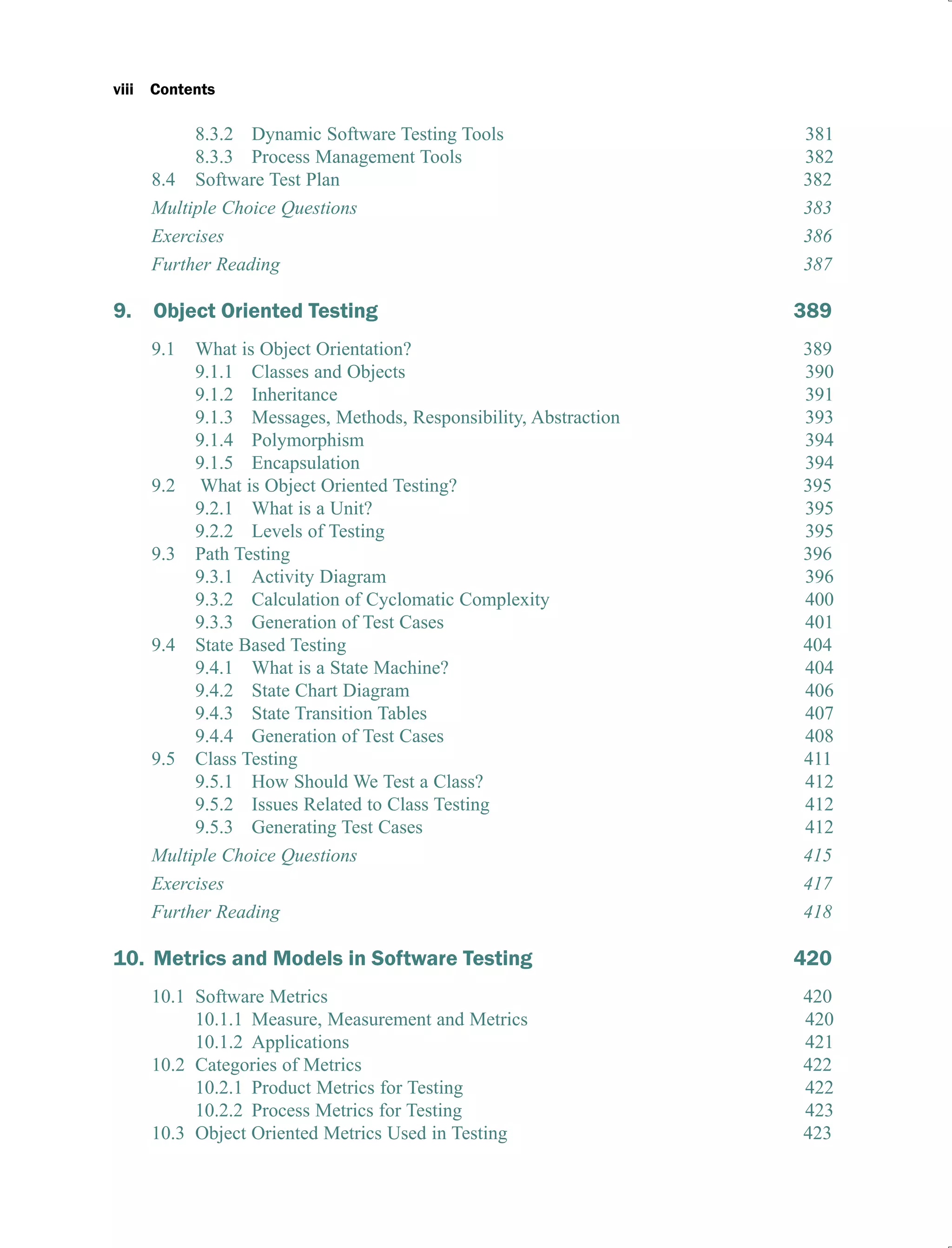
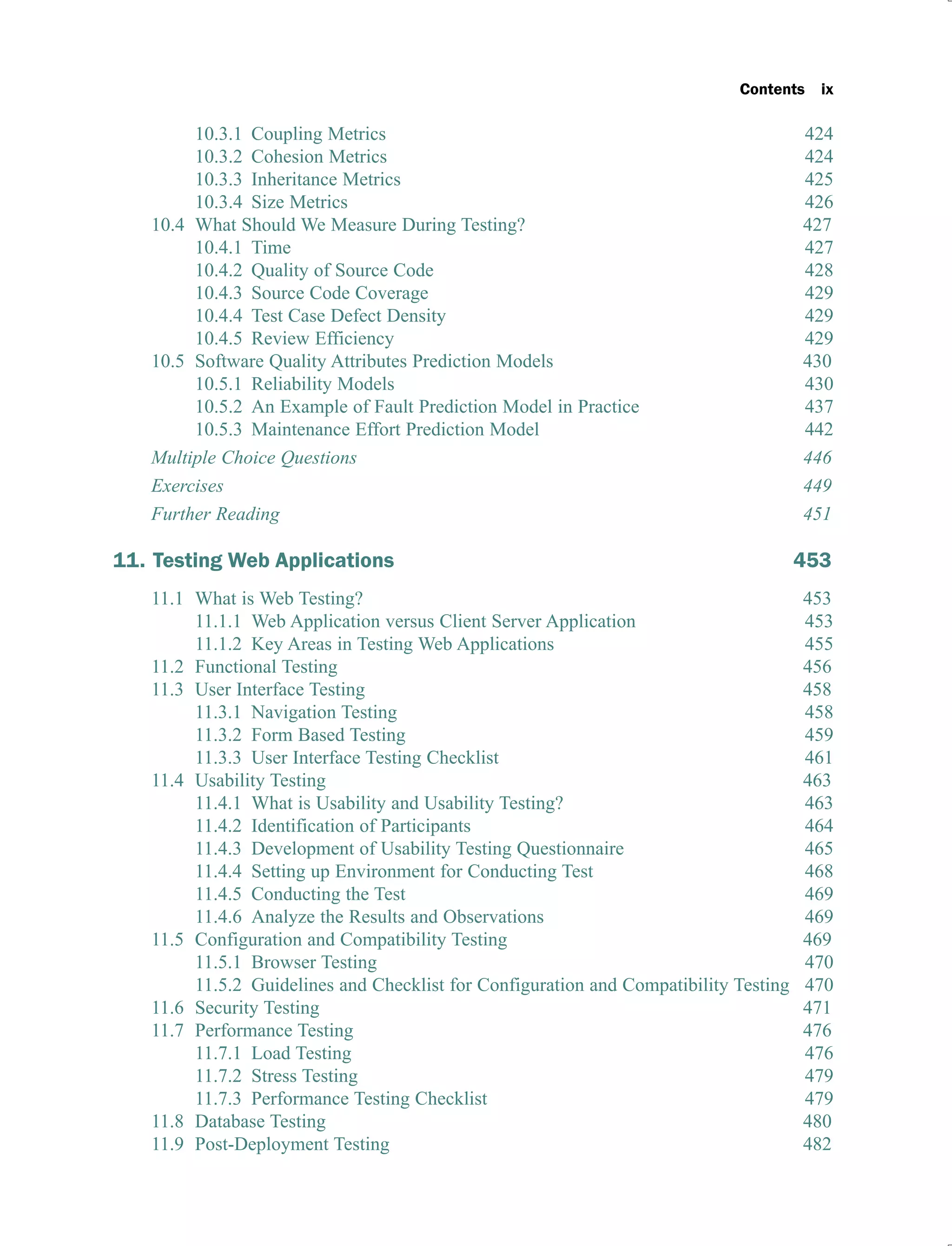
Contents
List of Figures xi
List of Tables xv
Preface xxi
Acknowledgements xxiii
1. Introduction 1
1.1 Some Software Failures 1
1.1.1 The Explosion of the Ariane 5 Rocket 1
1.1.2 The Y2K Problem 2
1.1.3 The USA Star-Wars Program 3
1.1.4 Failure of London Ambulance System 3
1.1.5 USS Yorktown Incident 3
1.1.6 Accounting Software Failures 3
1.1.7 Experience of Windows XP 4
1.2 Testing Process 4
1.2.1 What is Software Testing? 5
1.2.2 Why Should We Test? 14
1.2.3 Who Should We Do the Testing? 15
1.2.4 What Should We Test? 16
1.3 Some Terminologies 19
1.3.1 Program and Software 19
1.3.2 Verification and Validation 20
1.3.3 Fault, Error, Bug and Failure 21
1.3.4 Test, Test Case and Test Suite 21
1.3.5 Deliverables and Milestones 22
1.3.6 Alpha, Beta and Acceptance Testing 22
1.3.7 Quality and Reliability 23
iv Contents
1.3.8 Testing, Quality Assurance and Quality Control 23
1.3.9 Static and Dynamic Testing 23
1.3.10 Testing and Debugging 24
1.4 Limitations of Testing 24
1.4.1 Errors in the Software Requirement and Specification Document 24
1.4.2 Logical Bugs 24
1.4.3 Difficult to Measure the Progress of Testing 26
1.5 The V Shaped Software Life Cycle Model 26
1.5.1 Graphical Representation 27
1.5.2 Relationship of Development and Testing Parts 27
Multiple Choice Questions 28
Exercises 34
Further Reading 35
2. Functional Testing 37
2.1 Boundary Value Analysis 38
2.1.1 Robustness Testing 43
2.1.2 Worst-Case Testing 44
2.1.3 Robust Worst-Case Testing 46
2.1.4 Applicability 48
2.2 Equivalence Class Testing 63
2.2.1 Creation of Equivalence Classes 63
2.2.2 Applicability 65
2.3 Decision Table Based Testing 81
2.3.1 Parts of the Decision Table 81
2.3.2 Limited Entry and Extended Entry Decision Tables 82
2.3.3 ‘Do Not Care’ Conditions and Rule Count 82
2.3.4 Impossible Conditions 83
2.3.5 Applicability 83
2.4 Cause-Effect Graphing Technique 96
2.4.1 Identification of Causes and Effects 97
2.4.2 Design of Cause-Effect Graph 97
2.4.3 Use of Constraints in Cause-Effect Graph 97
2.4.4 Design of Limited Entry Decision Table 99
2.4.5 Writing of Test Cases 99
2.4.6 Applicability 99
Multiple Choice Questions 102
Exercises 105
Further Reading 108
3. Essentials of Graph Theory 110
3.1 What is a Graph? 110
3.1.1 Degree of a Node 112
3.1.2 Regular Graph 113
Contents v
3.2 Matrix Representation of Graphs 113
3.2.1 Incidence Matrix 114
3.2.2 Adjacency Matrix 114
3.3 Paths and Independent Paths 116
3.3.1 Cycles 117
3.3.2 Connectedness of a Graph 117
3.4 Generation of a Graph from Program 123
3.4.1 Program Graphs 124
3.4.2 DD Path Graphs 127
3.5 Identification of Independent Paths 144
3.5.1 Cyclomatic Complexity 144
3.5.2 Graph Matrices 150
Multiple Choice Questions 159
Exercises 161
Further Reading 163
4. Structural Testing 165
4.1 Control Flow Testing 165
4.1.1 Statement Coverage 166
4.1.2 Branch Coverage 167
4.1.3 Condition Coverage 167
4.1.4 Path Coverage 167
4.2 Data Flow Testing 173
4.2.1 Define/Reference Anomalies 174
4.2.2 Definitions 174
4.2.3 Identification of du and dc Paths 175
4.2.4 Testing Strategies Using du-Paths 175
4.2.5 Generation of Test Cases 176
4.3 Slice Based Testing 197
4.3.1 Guidelines for Slicing 197
4.3.2 Creation of Program Slices 198
4.3.3 Generation of Test Cases 202
4.4 Mutation Testing 212
4.4.1 Mutation and Mutants 212
4.4.2 Mutation Operators 216
4.4.3 Mutation Score 216
Multiple Choice Questions 223
Exercises 226
Further Reading 228
5. 0
5.1 Verification Methods 230
5.1.1 Peer Reviews 231
vi Contents
5.1.2 Walkthroughs 231
5.1.3 Inspections 231
5.1.4 Applications 232
5.2 Software Requirements Specification (SRS) Document Verification 233
5.2.1 Nature of the SRS Document 233
5.2.2 Characteristics and Organization of the SRS Document 233
5.2.3 SRS Document Checklist 235
5.3 Software Design Description (SDD) Document Verification 238
5.3.1 Organization of the SDD Document 239
5.3.2 The SDD Document Checklist 239
5.4 Source Code Reviews 241
5.4.1 Issues Related to Source Code Reviews 241
5.4.2 Checklist of Source Code Reviews 242
5.5 User Documentation Verification 243
5.5.1 Review Process Issues 244
5.5.2 User Documentation Checklist 244
5.6 Software Project Audit 245
5.6.1 Relevance Scale 246
5.6.2 Theory and Practice Scale 246
5.6.3 Project Audit and Review Checklist 246
5.7 Case Study 257
Multiple Choice Questions 279
Exercises 282
Further Reading 283
6. Creating Test Cases from Requirements and Use Cases 285
6.1 Use Case Diagram and Use Cases 285
6.1.1 Identification of Actors 286
6.1.2 Identification of Use Cases 287
6.1.3 Drawing of Use Case Diagram 288
6.1.4 Writing of Use Case Description 290
6.2 Generation of Test Cases from Use Cases 292
6.2.1 Generation of Scenario Diagrams 293
6.2.2 Creation of Use Case Scenario Matrix 294
6.2.3 Identification of Variables in a Use Case 295
6.2.4 Identification of Different Input States of a Variable 296
6.2.5 Design of Test Case Matrix 296
6.2.6 Assigning Actual Values to Variables 296
6.3 Guidelines for generating validity checks 316
6.3.1 Data Type 316
6.3.2 Data Range 316
6.3.3 Special Data Conditions 316
6.3.4 Mandatory Data Inputs 316
6.3.5 Domain Specific Checks 316
6.4 Strategies for Data Validity 317
6.4.1 Accept Only Known Valid Data 317
Contents vii
6.4.2 Reject Known Bad Data 322
6.4.3 Sanitize All Data 322
6.5 Database Testing 326
Multiple Choice Questions 331
Exercises 333
Further Reading 334
7. Selection, Minimization and Prioritization of Test Cases for
Regression Testing 335
7.1 What is Regression Testing? 335
7.1.1 Regression Testing Process 336
7.1.2 Selection of Test Cases 337
7.2 Regression Test Cases Selection 339
7.2.1 Select All Test Cases 339
7.2.2 Select Test Cases Randomly 339
7.2.3 Select Modification Traversing Test Cases 339
7.3 Reducing the Number of Test Cases 340
7.3.1 Minimization of Test Cases 340
7.3.2 Prioritization of Test Cases 341
7.4 Risk Analysis 342
7.4.1 What is Risk? 342
7.4.2 Risk Matrix 343
7.5 Code Coverage Prioritization Technique 346
7.5.1 Test Cases Selection Criteria 347
7.5.2 Modification Algorithm 347
7.5.3 Deletion Algorithm 352
Multiple Choice Questions 363
Exercises 364
Further Reading 365
8. Software Testing Activities 368
8.1 Levels of Testing 368
8.1.1 Unit Testing 369
8.1.2 Integration Testing 370
8.1.3 System Testing 373
8.1.4 Acceptance Testing 373
8.2 Debugging 374
8.2.1 Why Debugging is so Difficult? 374
8.2.2 Debugging Process 375
8.2.3 Debugging Approaches 377
8.2.4 Debugging Tools 378
8.3 Software Testing Tools 379
8.3.1 Static Software Testing Tools 379
viii Contents
8.3.2 Dynamic Software Testing Tools 381
8.3.3 Process Management Tools 382
8.4 Software Test Plan 382
Multiple Choice Questions 383
Exercises 386
Further Reading 387
9. Object Oriented Testing 389
9.1 What is Object Orientation? 389
9.1.1 Classes and Objects 390
9.1.2 Inheritance 391
9.1.3 Messages, Methods, Responsibility, Abstraction 393
9.1.4 Polymorphism 394
9.1.5 Encapsulation 394
9.2 What is Object Oriented Testing? 395
9.2.1 What is a Unit? 395
9.2.2 Levels of Testing 395
9.3 Path Testing 396
9.3.1 Activity Diagram 396
9.3.2 Calculation of Cyclomatic Complexity 400
9.3.3 Generation of Test Cases 401
9.4 State Based Testing 404
9.4.1 What is a State Machine? 404
9.4.2 State Chart Diagram 406
9.4.3 State Transition Tables 407
9.4.4 Generation of Test Cases 408
9.5 Class Testing 411
9.5.1 How Should We Test a Class? 412
9.5.2 Issues Related to Class Testing 412
9.5.3 Generating Test Cases 412
Multiple Choice Questions 415
Exercises 417
Further Reading 418
10. Metrics and Models in Software Testing 420
10.1 Software Metrics 420
10.1.1 Measure, Measurement and Metrics 420
10.1.2 Applications 421
10.2 Categories of Metrics 422
10.2.1 Product Metrics for Testing 422
10.2.2 Process Metrics for Testing 423
10.3 Object Oriented Metrics Used in Testing 423
Contents ix
10.3.1 Coupling Metrics 424
10.3.2 Cohesion Metrics 424
10.3.3 Inheritance Metrics 425
10.3.4 Size Metrics 426
10.4 What Should We Measure During Testing? 427
10.4.1 Time 427
10.4.2 Quality of Source Code 428
10.4.3 Source Code Coverage 429
10.4.4 Test Case Defect Density 429
10.4.5 Review Efficiency 429
10.5 Software Quality Attributes Prediction Models 430
10.5.1 Reliability Models 430
10.5.2 An Example of Fault Prediction Model in Practice 437
10.5.3 Maintenance Effort Prediction Model 442
Multiple Choice Questions 446
Exercises 449
Further Reading 451
11. Testing Web Applications 453
11.1 What is Web Testing? 453
11.1.1 Web Application versus Client Server Application 453
11.1.2 Key Areas in Testing Web Applications 455
11.2 Functional Testing 456
11.3 User Interface Testing 458
11.3.1 Navigation Testing 458
11.3.2 Form Based Testing 459
11.3.3 User Interface Testing Checklist 461
11.4 Usability Testing 463
11.4.1 What is Usability and Usability Testing? 463
11.4.2 Identification of Participants 464
11.4.3 Development of Usability Testing Questionnaire 465
11.4.4 Setting up Environment for Conducting Test 468
11.4.5 Conducting the Test 469
11.4.6 Analyze the Results and Observations 469
11.5 Configuration and Compatibility Testing 469
11.5.1 Browser Testing 470
11.5.2 Guidelines and Checklist for Configuration and Compatibility Testing 470
11.6 Security Testing 471
11.7 Performance Testing 476
11.7.1 Load Testing 476
11.7.2 Stress Testing 479
11.7.3 Performance Testing Checklist 479
11.8 Database Testing 480
11.9 Post-Deployment Testing 482
x Contents
11.10 Web Metrics 485
Multiple Choice Questions 486
Exercises 490
Further Reading 492
12. Automated Test Data Generation 494
12.1 What is Automated Test Data Generation? 494
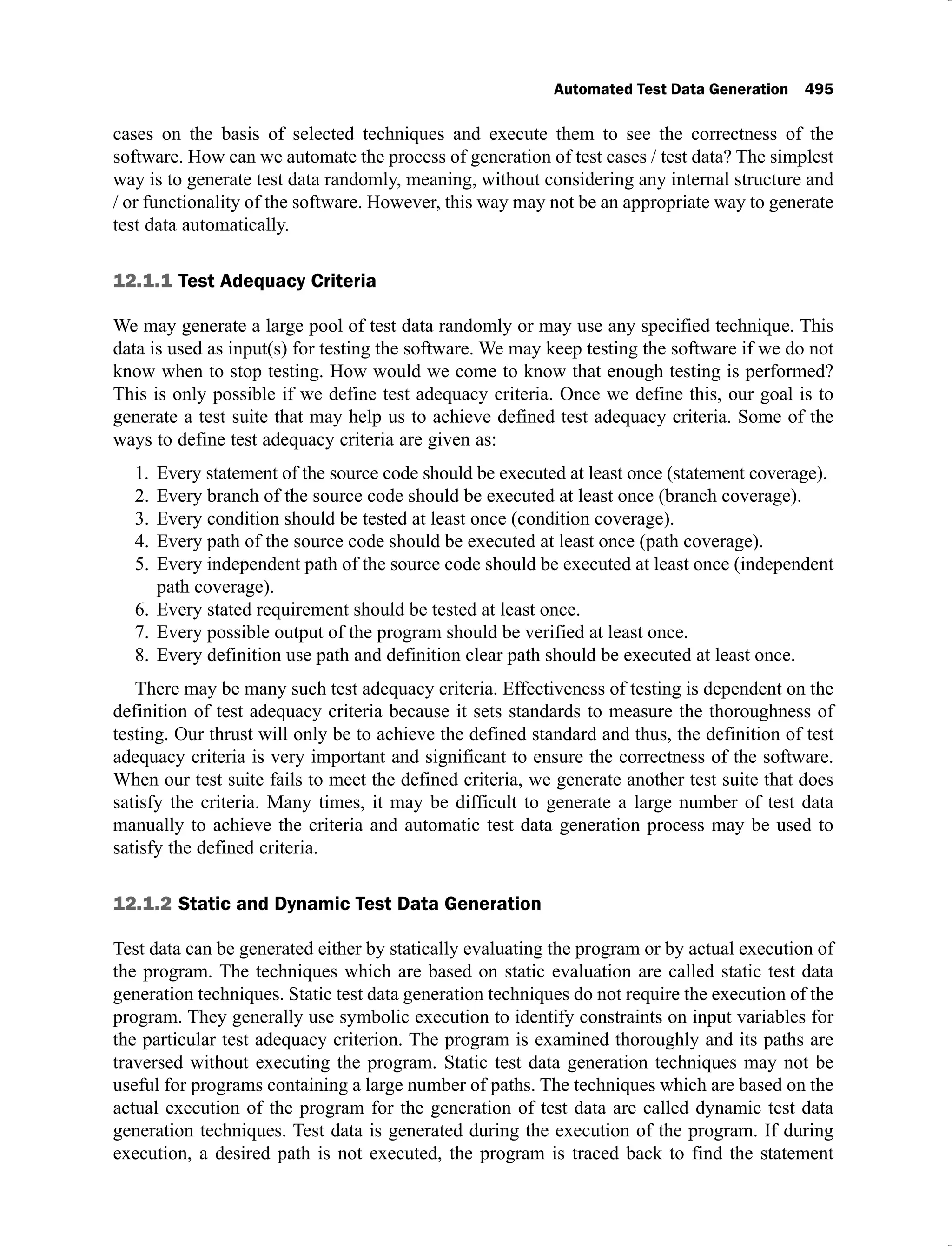
12.1.1 Test Adequacy Criteria 495
12.1.2 Static and Dynamic Test Data Generation 495
12.2 Approaches to Test Data Generation 496
12.2.1 Random Testing 496
12.2.2 Symbolic Execution 496
12.2.3 Dynamic Test Data Generation 501
12.3 Test Data Generation using Genetic Algorithm 502
12.3.1 Initial Population 503
12.3.2 Crossover and Mutation 503
12.3.3 Fitness Function 504
12.3.4 Selection 505
12.3.5 Algorithm for Generating Test Data 505
12.4 Test Data Generation Tools 511
Multiple Choice Questions 512
Exercises 513
Further Reading 514
Appendix I 517
Appendix II 541
Appendix III 594
References 612
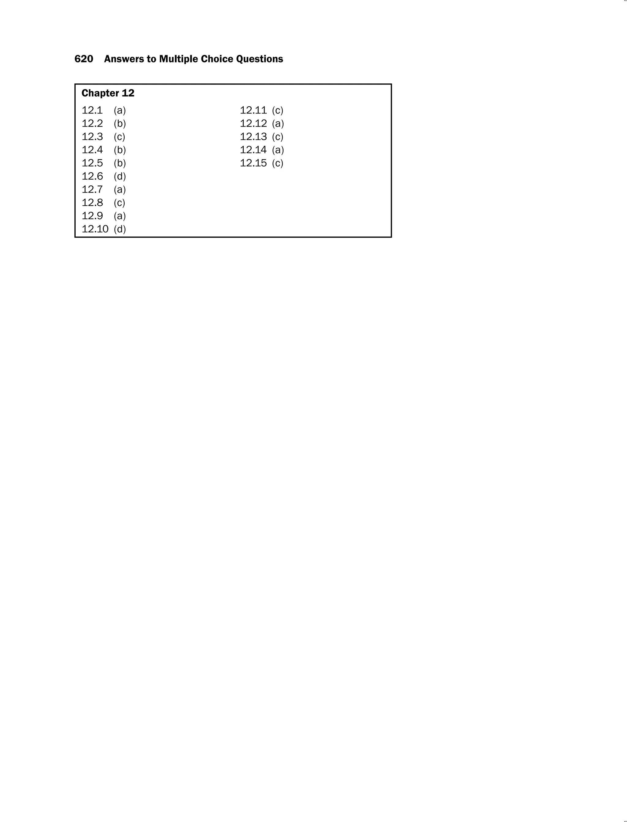
Answers to Multiple Choice Questions 617
Index 621
List of Figures
1.1 Program ‘Minimum’ to find the smallest integer out of a set of integers 5
1.2 Modified program ‘Minimum’ to find the smallest integer out of a set of integers 11
1.3 Final program ‘Minimum’ to find the smallest integer out of a set of integers 13
1.4 Phase wise cost of fixing an error 15
1.5 Control flow graph of a 10 to 20 statement program [MYER04] 18
1.6 Components of the software 19
1.7 Documentation manuals 19
1.8 Operating system manuals 20
1.9 A typical example 25
1.10 V shaped software development life cycle model 27
2.1 Functional (Black Box) testing 37
2.2 Five values for input ‘x’ of ‘Square’ program 38
2.3 Selected values for input values x and y 39
2.4 Valid input domain for the program ‘Addition’ 39
2.5 Graphical representation of inputs 40
2.6 Graphical representation of inputs 44
2.7 Graphical representation of inputs 45
2.8 Graphical representation of inputs 46
2.9 Graphical representation of inputs 64
2.10 Equivalence classes of input domain 65
2.11 Steps for the generation of test cases 96
2.12 Basic notations used in cause-effect graph 97
2.13 Constraint symbols for any cause-effect graph 98
2.14 Example of cause-effect graph with exclusive (constraint) and requires constraint 99
2.15 Cause-effect graph of rental car problem 100
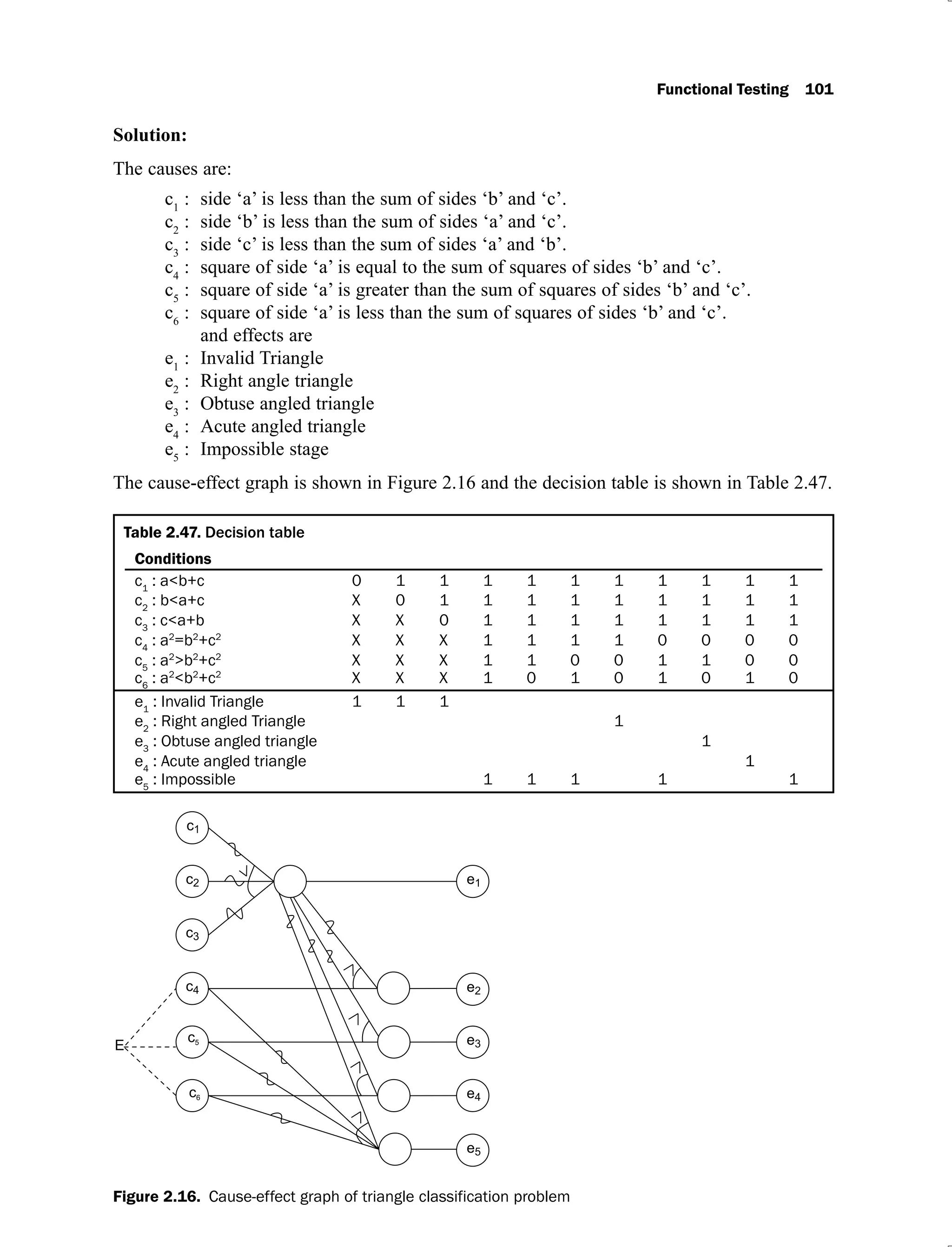
2.16 Cause-effect graph of triangle classification problem 101
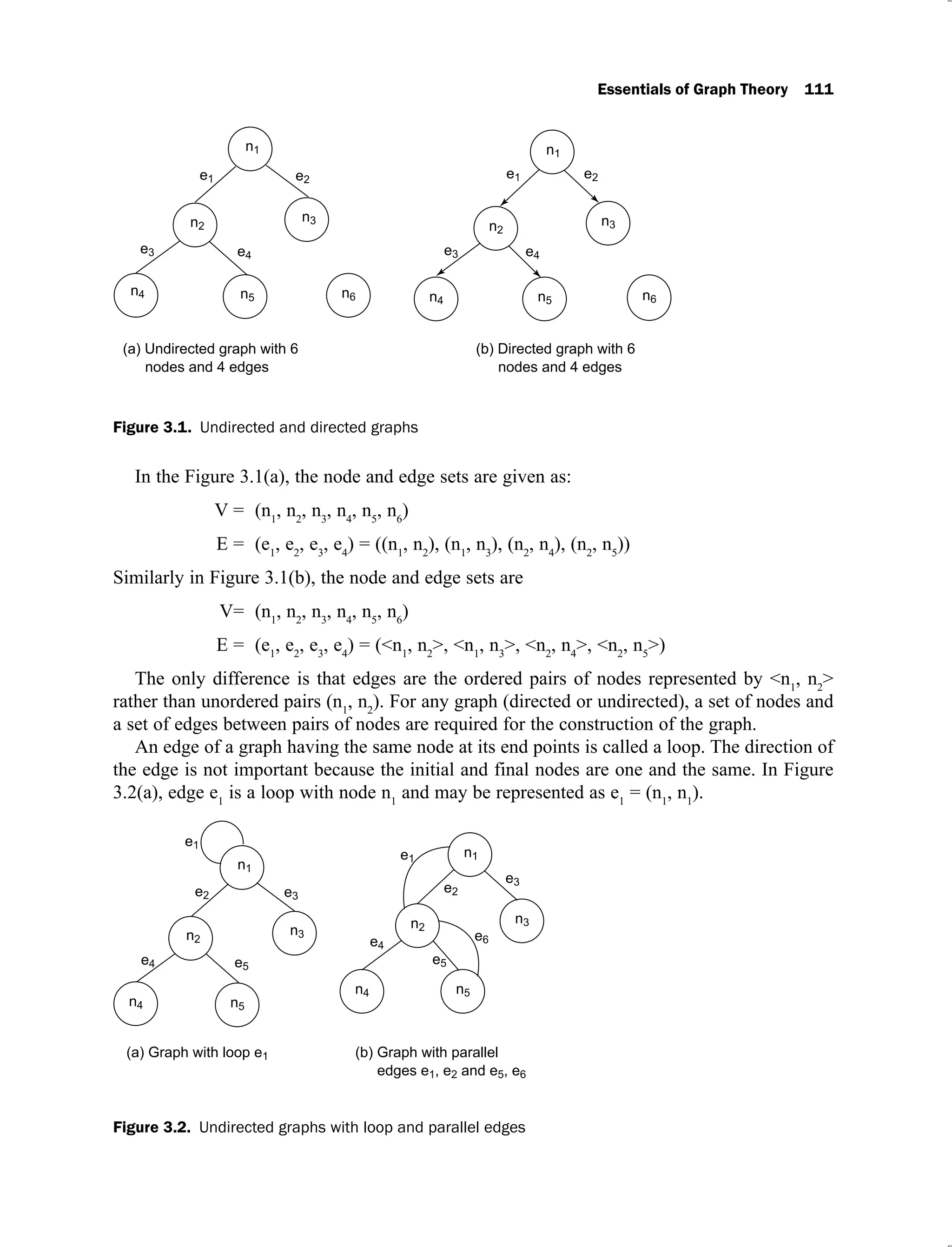
3.1 Undirected and directed graphs 111
3.2 Graphs with loop and parallel edges 111
3.3 Types of graphs 112
3.4 Regular graphs 113
3.5 Cyclic graph 117
3.6 Disconnected graphs 118
3.7 Strongly connected graph 118
3.8 Weakly connected graph 119
xii List of Figures
3.9 Basic constructs of a program graph 124
3.10 Program ‘Square’ and its program graph 125
3.11 Program to find the largest among three numbers 126
3.12 Program graph to find the largest number amongst three numbers as given
in Figure 3.11 126
3.13 DD path graph and mapping table of program graph in Figure 3.10 127
3.14 DD path graph of the program to find the largest among three numbers 128
3.15 Source code of determination of division of a student problem 130
3.16 Program graph 130
3.17 DD path graph of program to find division of a student 132
3.18 Source code for classification of triangle problem 134
3.19 Program graph of classification of triangle problem 134
3.20 DD path graph of the program to classify a triangle 136
3.21 Source code for determination of day of the week 139
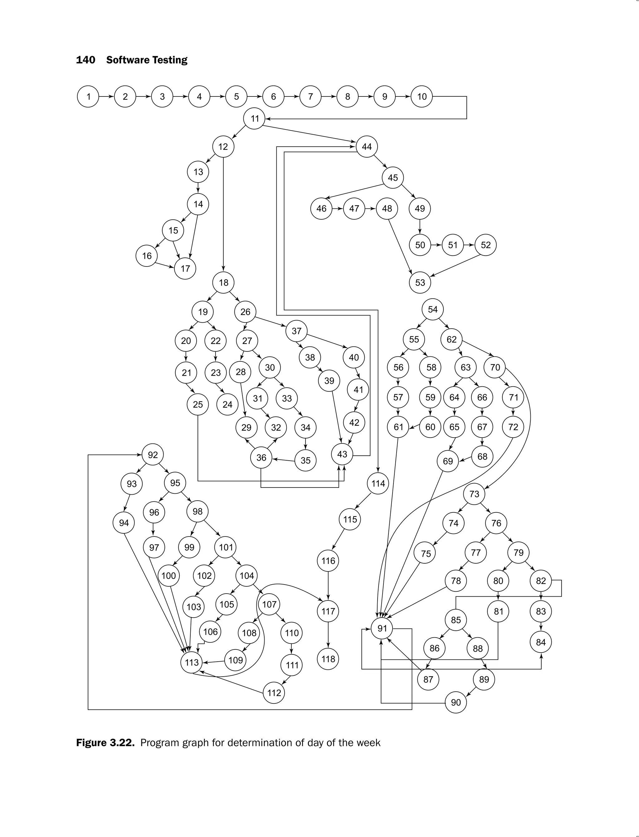
3.22 Program graph for determination of day of the week 140
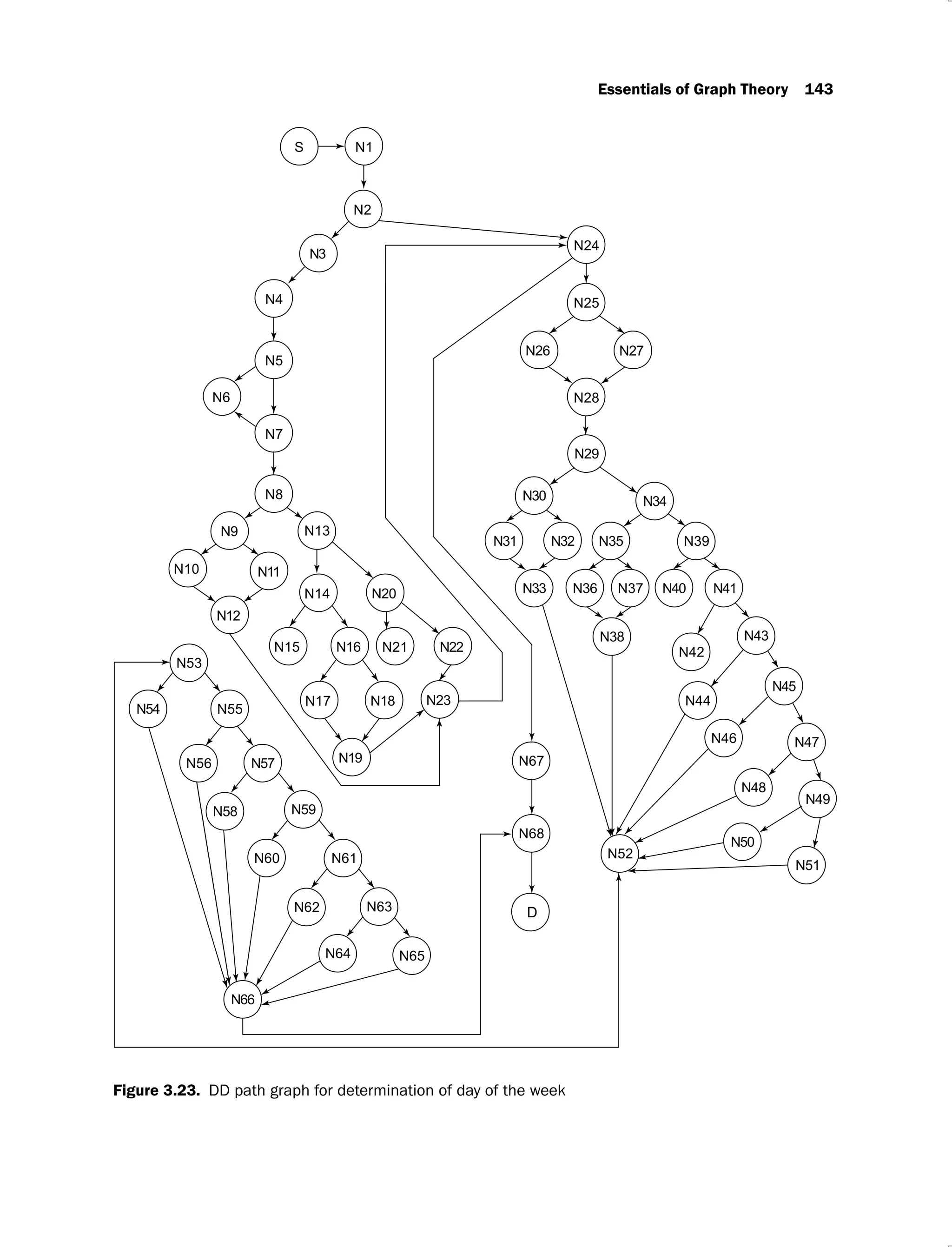
3.23 DD path graph for determination of day of the week 143
3.24 Program graph 145
3.25 Program graph with 3 connected components 146
3.26 Program graphs and graph matrices 151
3.27 Connection matrix for program graph shown in Figure 3.26(b) 152
3.28 Various paths of program graph given in Figure 3.26(a) 153
3.29 Program graph 154
3.30 DD path graph for determination of division problem 155
3.31 Graph matrix for determination of division problem 156
3.32 Connection matrix for determination of division problem 156
3.33 DD path graph for classification of triangle problem 157
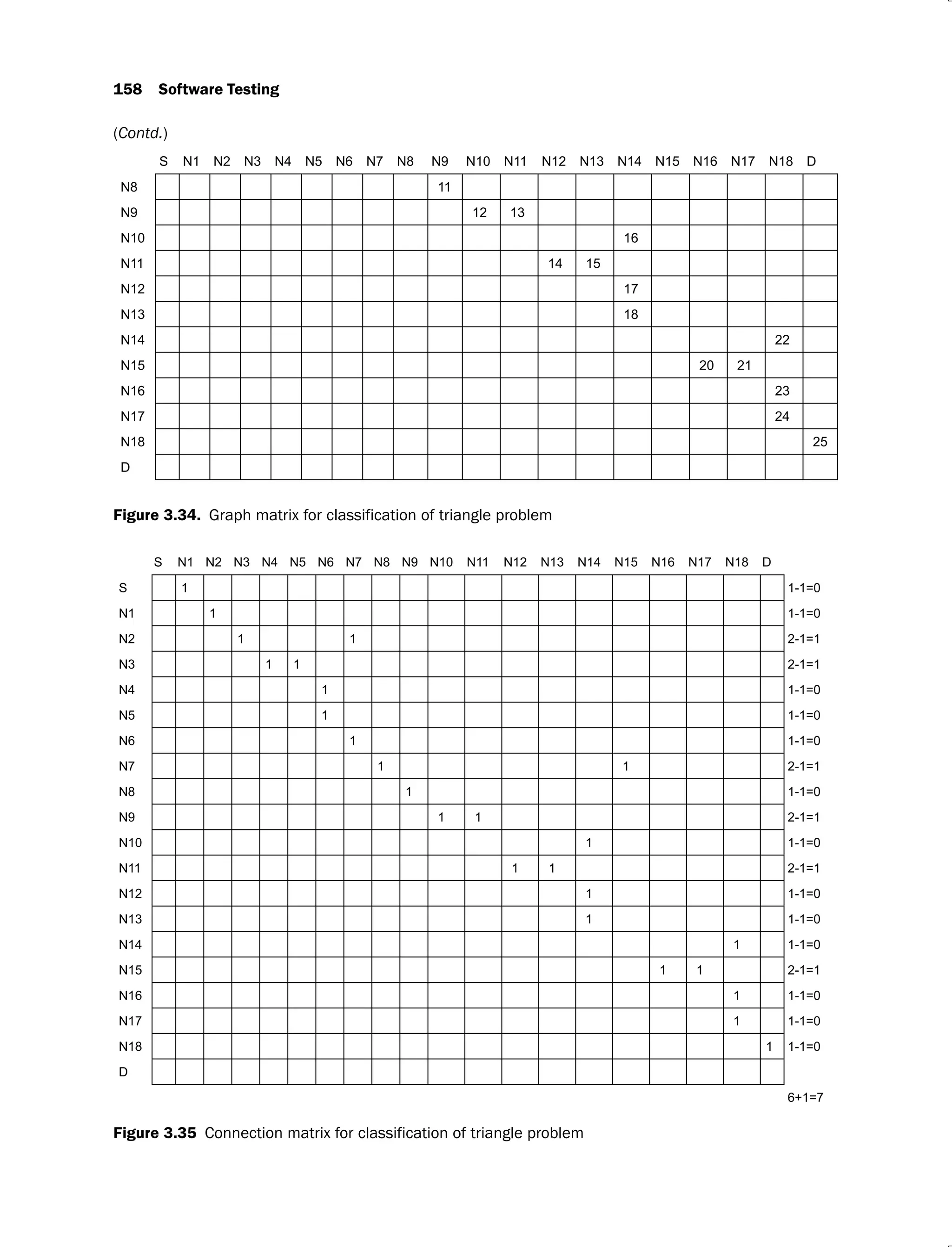
3.34 Graph matrix for classification of triangle problem 158
3.35 Connection matrix for classification of triangle problem 158
4.1 Source code with program graph 166
4.2 Portion of a program 198
4.3 Two slices for variable ‘c’ 199
4.4 Example program 199
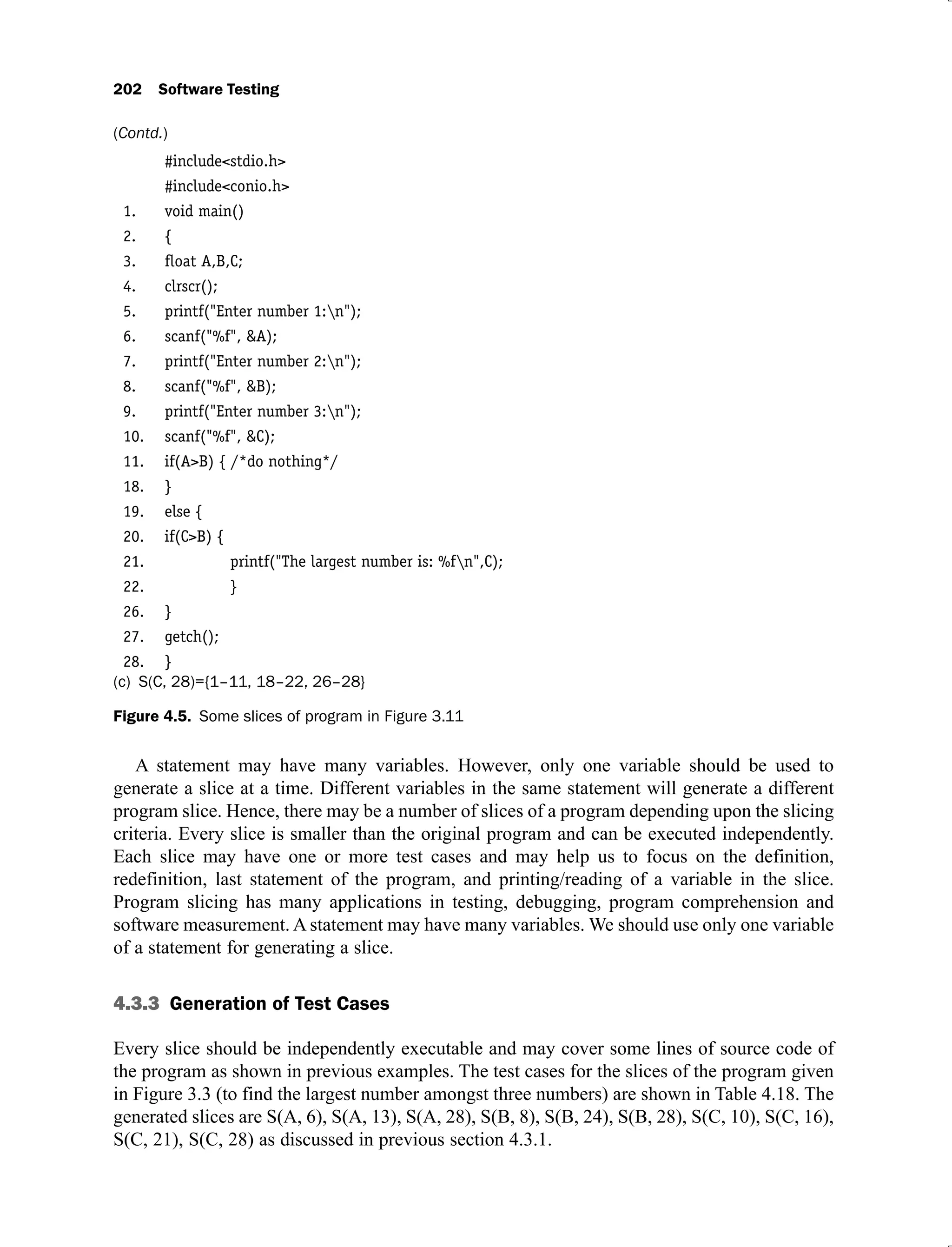
4.5 Some slices of program in Figure 3.11 202
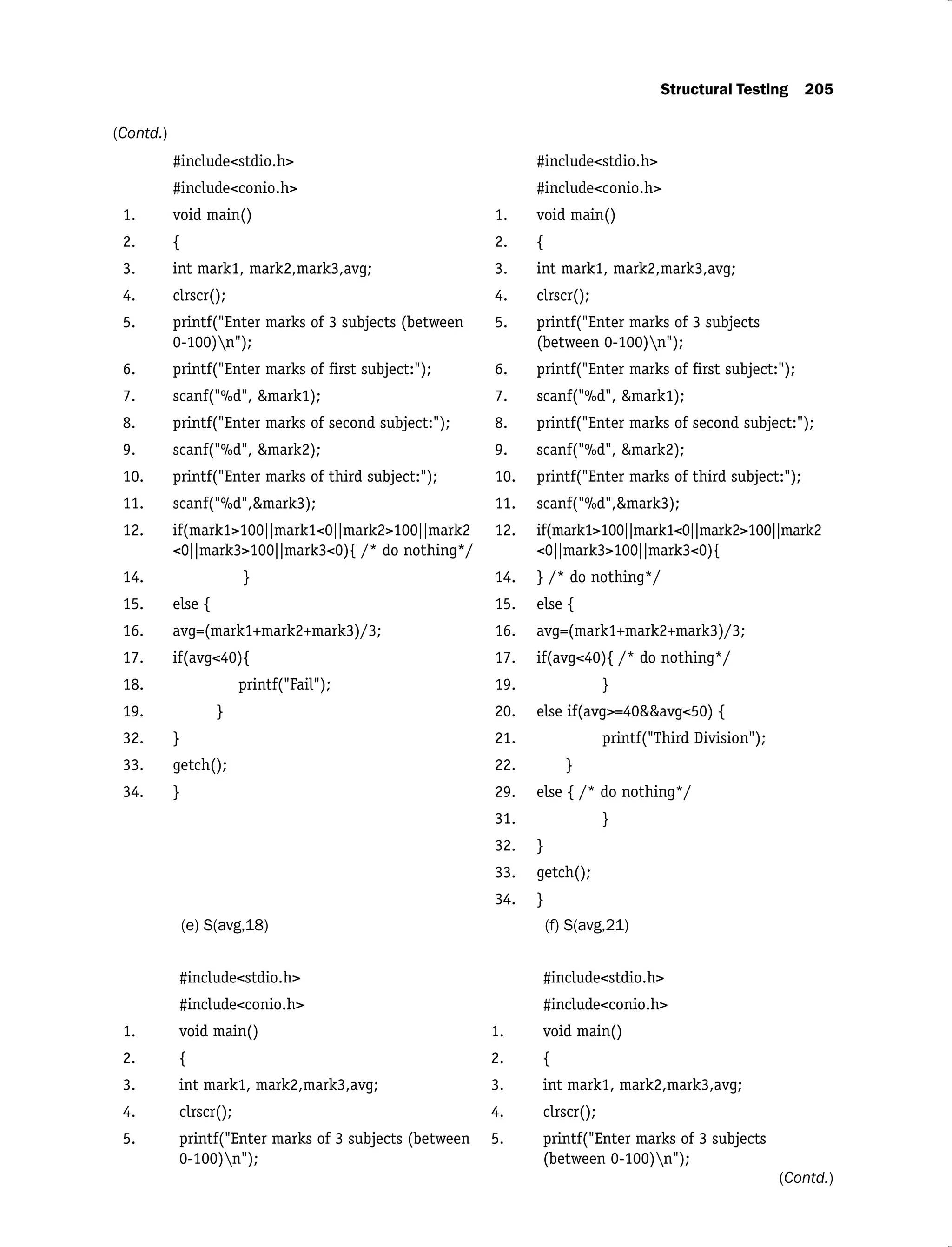
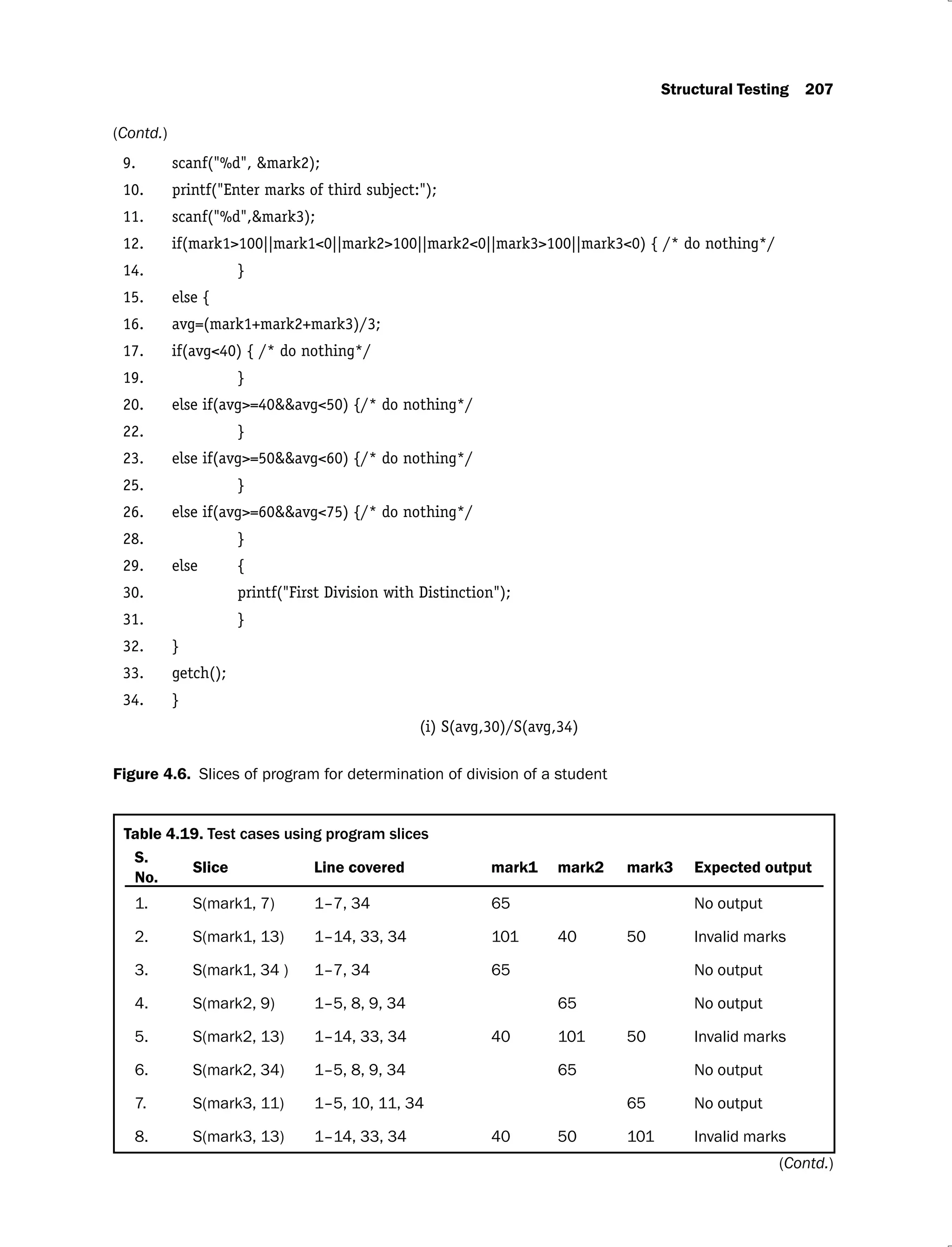
4.6 Slices of program for determination of division of a student 207
4.7 Mutant1
(M1
) of program to find the largest among three numbers 214
4.8 Mutant2
(M2
) of program to find the largest among three numbers 214
4.9 Mutant3
(M3
) of program to find the largest among three numbers 215
6.1 Components of use case diagram 288
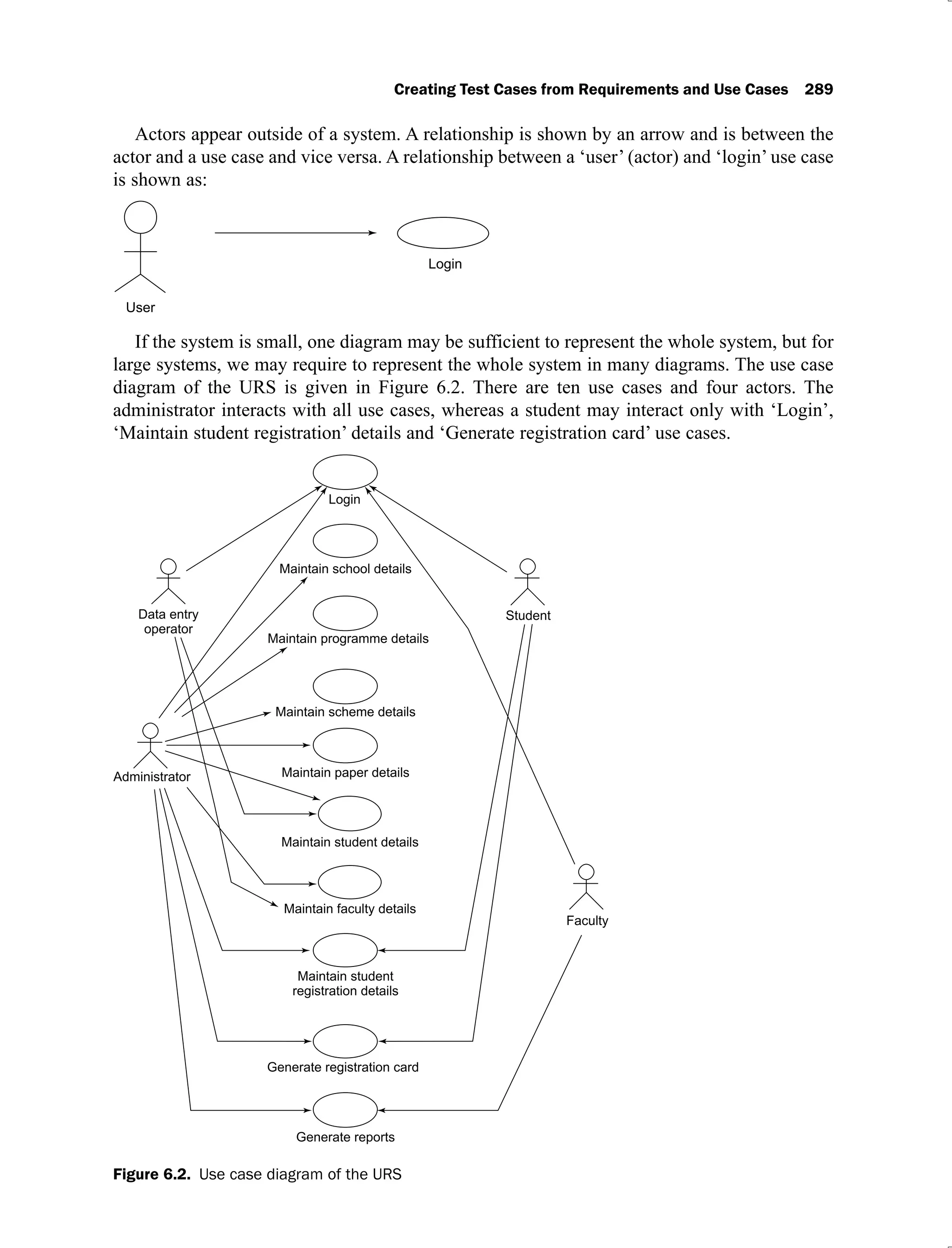
6.2 Use case diagram of the URS 289
6.3 Basic and alternative flows with pre-and post-conditions 293
6.4 Basic and alternative flows for login use case (a) Login (b) Change password 294
6.5 Basic and alternative flows for ‘maintain school’, ‘programme’, ‘scheme’,
‘paper’, or ‘student details’ use cases (a) Add details (b) Edit details (c) Delete
details (d) View details 301
6.6 Login form 318
6.7 Change password form 320
List of Figures xiii
6.8 Maintain school details form 322
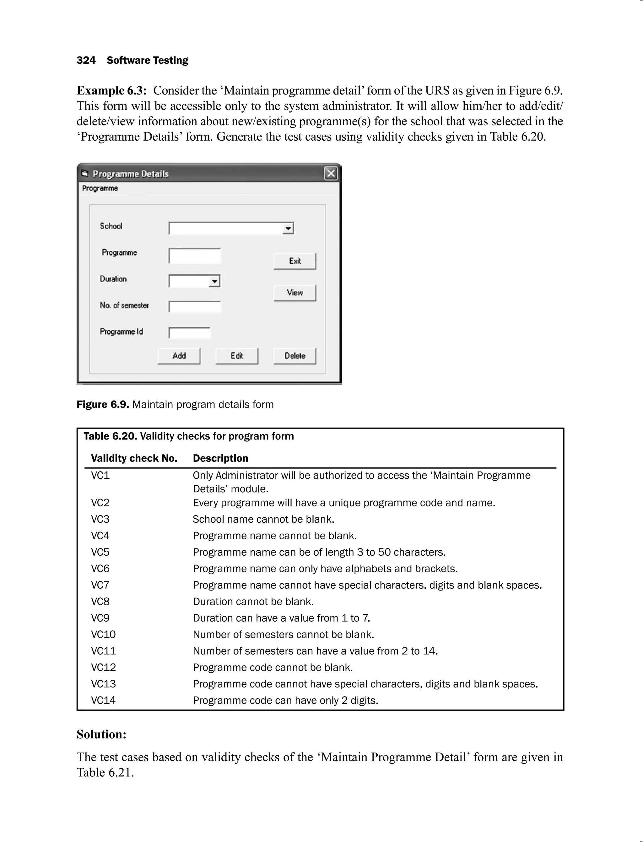
6.9 Maintain program details form 324
7.1 Steps of regression testing process 337
7.2 Program for printing value of z 338
7.3 Threshold by quadrant 343
7.4 Alternate threshold by quadrant 344
7.5 Threshold by diagonal quadrant 345
7.6 Threshold based on high ‘Impact of Problem’ value 345
7.7 Threshold based on high ‘probability of occurrence of problem’ value 346
8.1 Levels of testing 369
8.2 Unit under test with stubs and driver 370
8.3 Coupling amongst units 371
8.4 Integration approaches 372
9.1 Class and its objects 390
9.2 Class courier 391
9.3 The categories around fast track courier 392
9.4 A class hierarchy 393
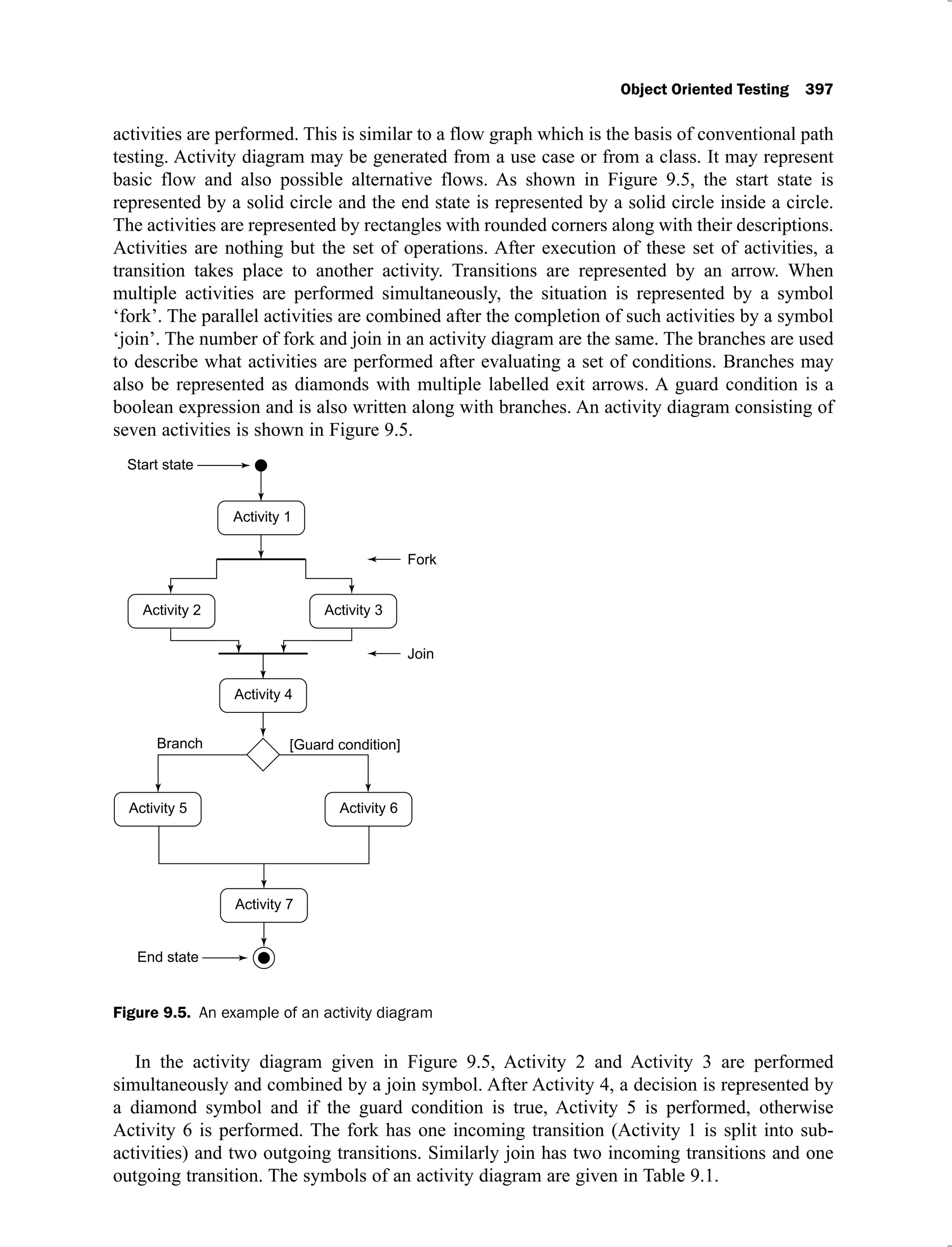
9.5 An example of an activity diagram 397
9.6 Program to determine division of a student 399
9.7 Activity diagram of function validate() 400
9.8 Activity diagram of function calculate() 400
9.9 Program to determine largest among three numbers 403
9.10 Activity diagram for function validate() 403
9.11 Activity diagram for function maximum() 404
9.12 A typical state machine diagram 405
9.13 Typical life cycle of a process 406
9.14 State chart diagram for class stack 407
9.15 State chart diagram of withdrawal from ATM 410
9.16 Specification for the class stack 413
9.17 Class ATM withdrawal 414
10.1 as a function of 431
10.2 Relationship between and μ 431
10.3 Relationship between and 432
10.4 ROC curve for (a) Model I (b) Model II (c) Model III (d) Model IV using
LR method 442
10.5 Comparison between actual and predicted values for maintenance effort 446
11.1 Two-tier architecture of client-server application 454
11.2 Three-tier architecture of web based applications 454
11.3 Web application process 455
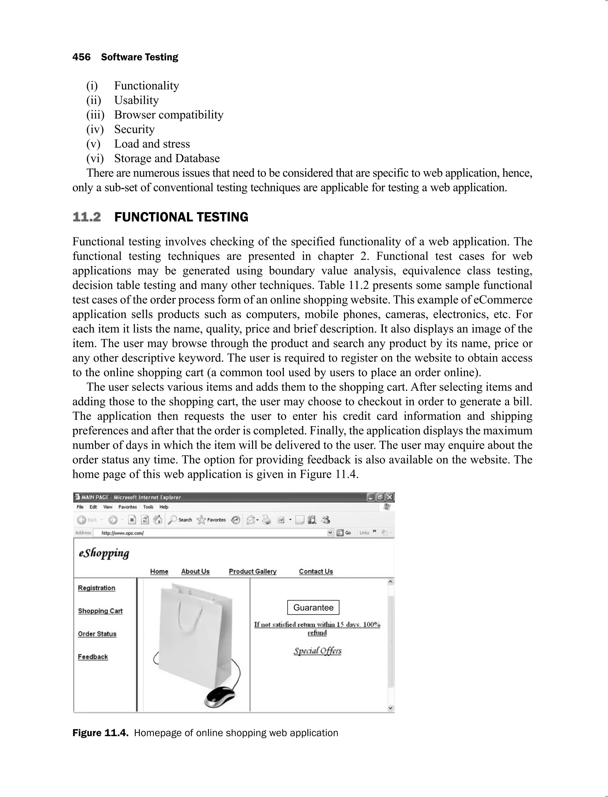
11.4 Homepage of online shopping web application 456
11.5 Sample online registration form 460
11.6 Usability testing steps 464
11.7 Participant characteristics for online shopping website 464
11.8 Usability testing questionnaire 468
11.9 Sample questions for online shopping website 468
xiv List of Figures
11.10 Security threats 472
11.11 Working of a firewall 473
11.12 Post deployment testing questionnaire 484
11.13 Typical post deployment testing procedure of a web application 484
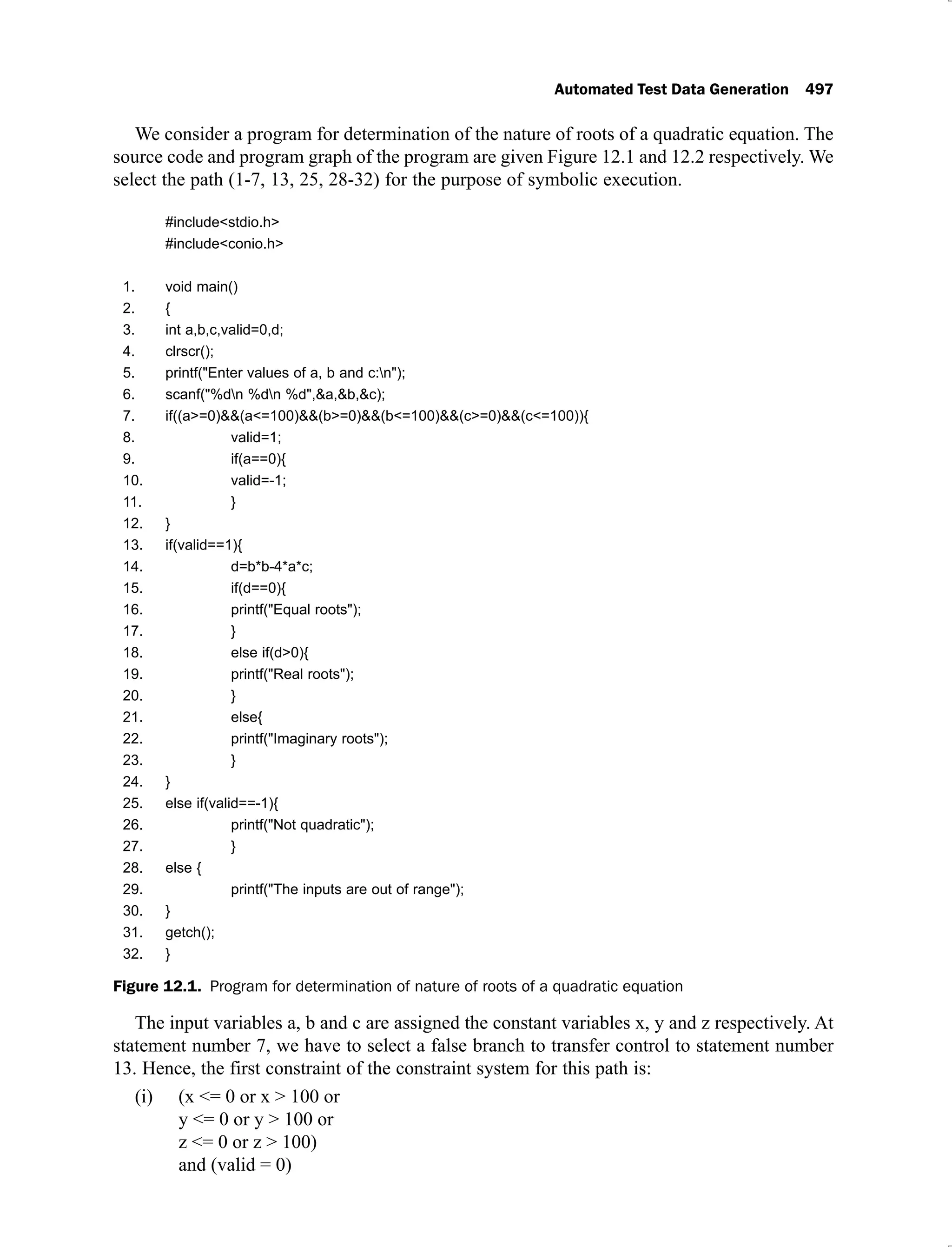
12.1 Program for determination of nature of roots of a quadratic equation 497
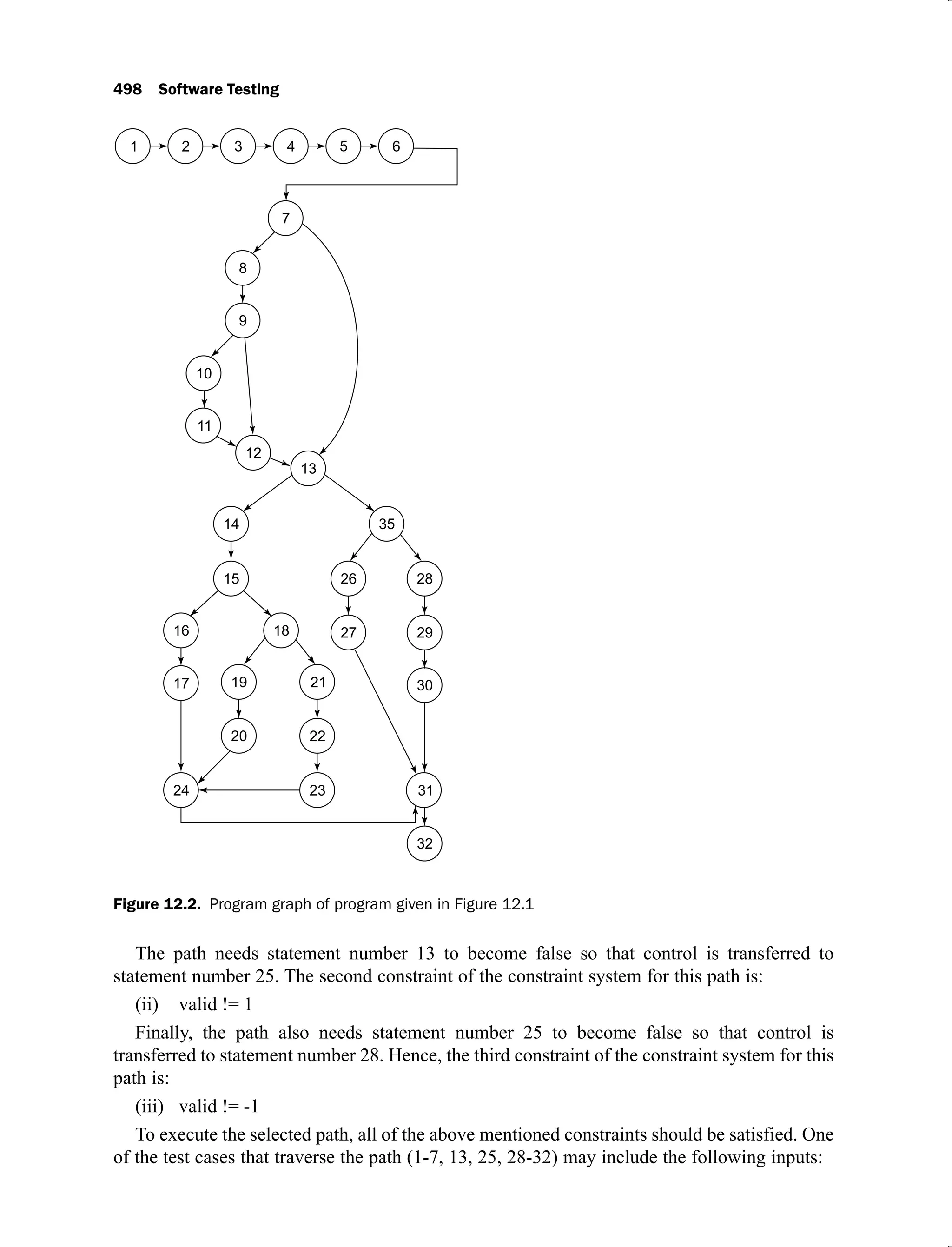
12.2 Program graph of program given in Figure 12.1 498
12.3 A typical program 501
12.4 Flow chart of various steps of genetic algorithm 506
12.5 Program to divide two numbers 507
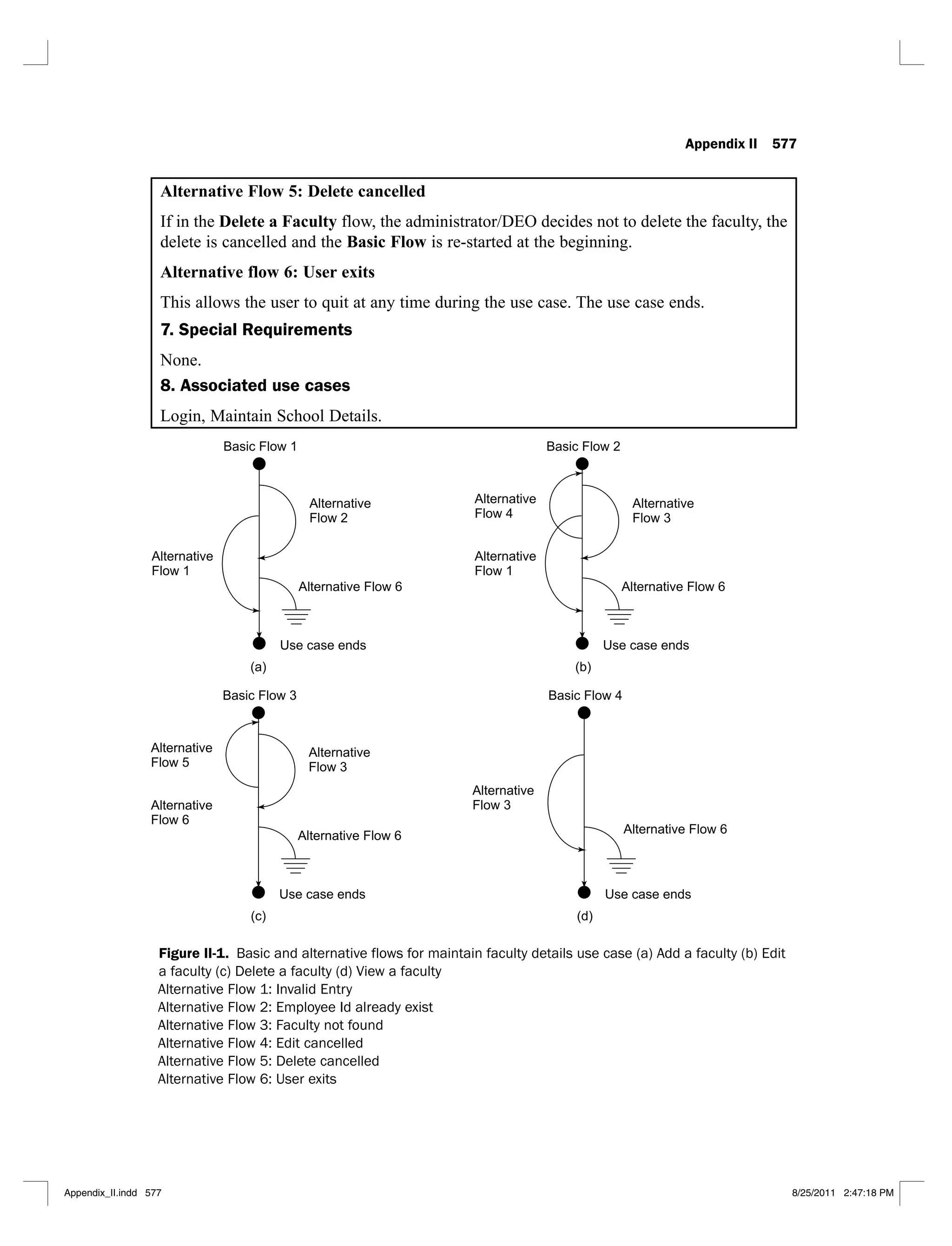
II-1 Basic and alternative flows for maintain faculty details use case (a) Add a faculty
(b) Edit a faculty (c) Delete a faculty (d) View a faculty 577
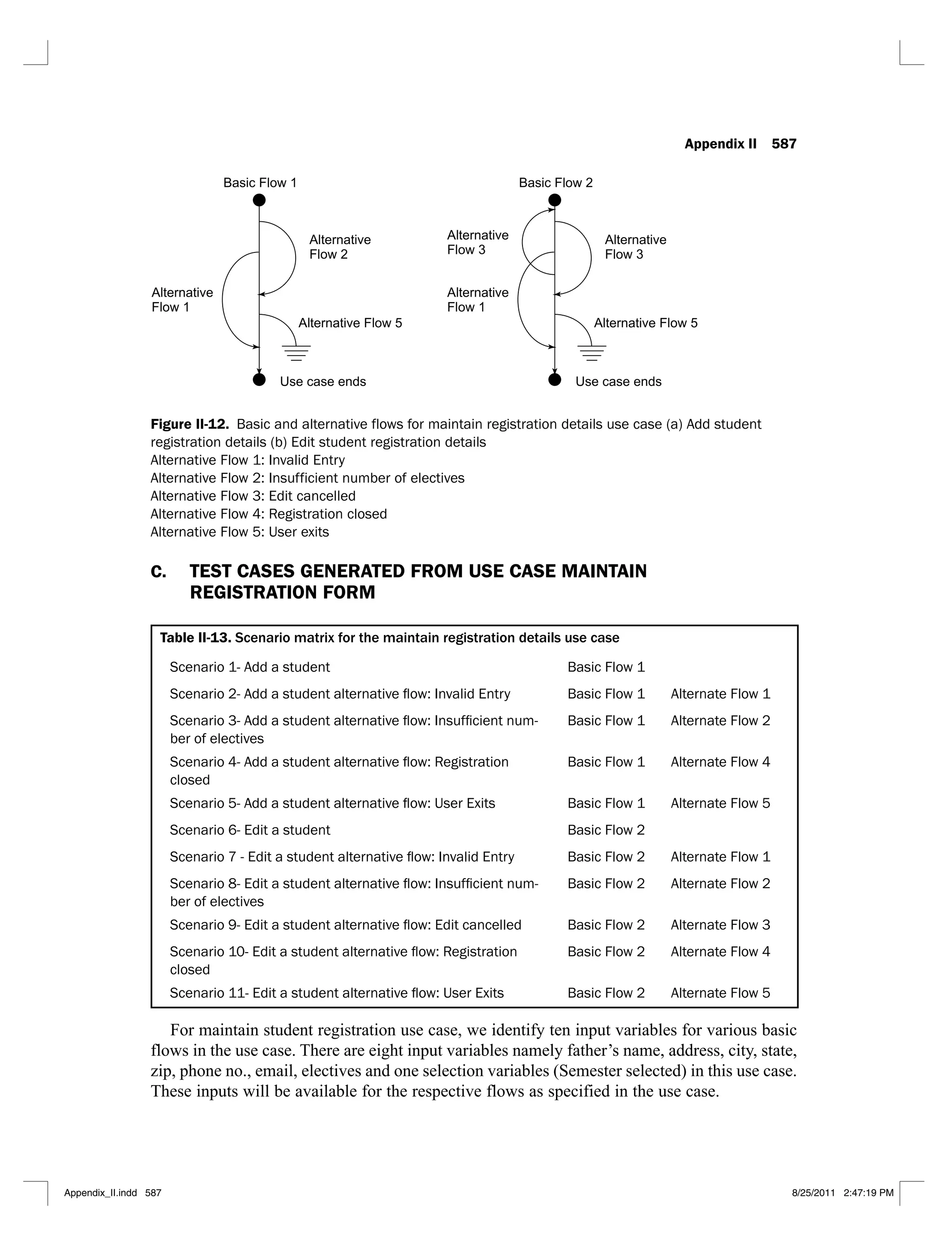
II-2 Basic and alternative flows for maintain registration details use case
(a) Add student registration details (b) Edit student registration details 587
III-1 Validity checks for scheme form 595
III-2 Test case with actual data values for the scheme form 597
III-3 Validity checks for paper form 598
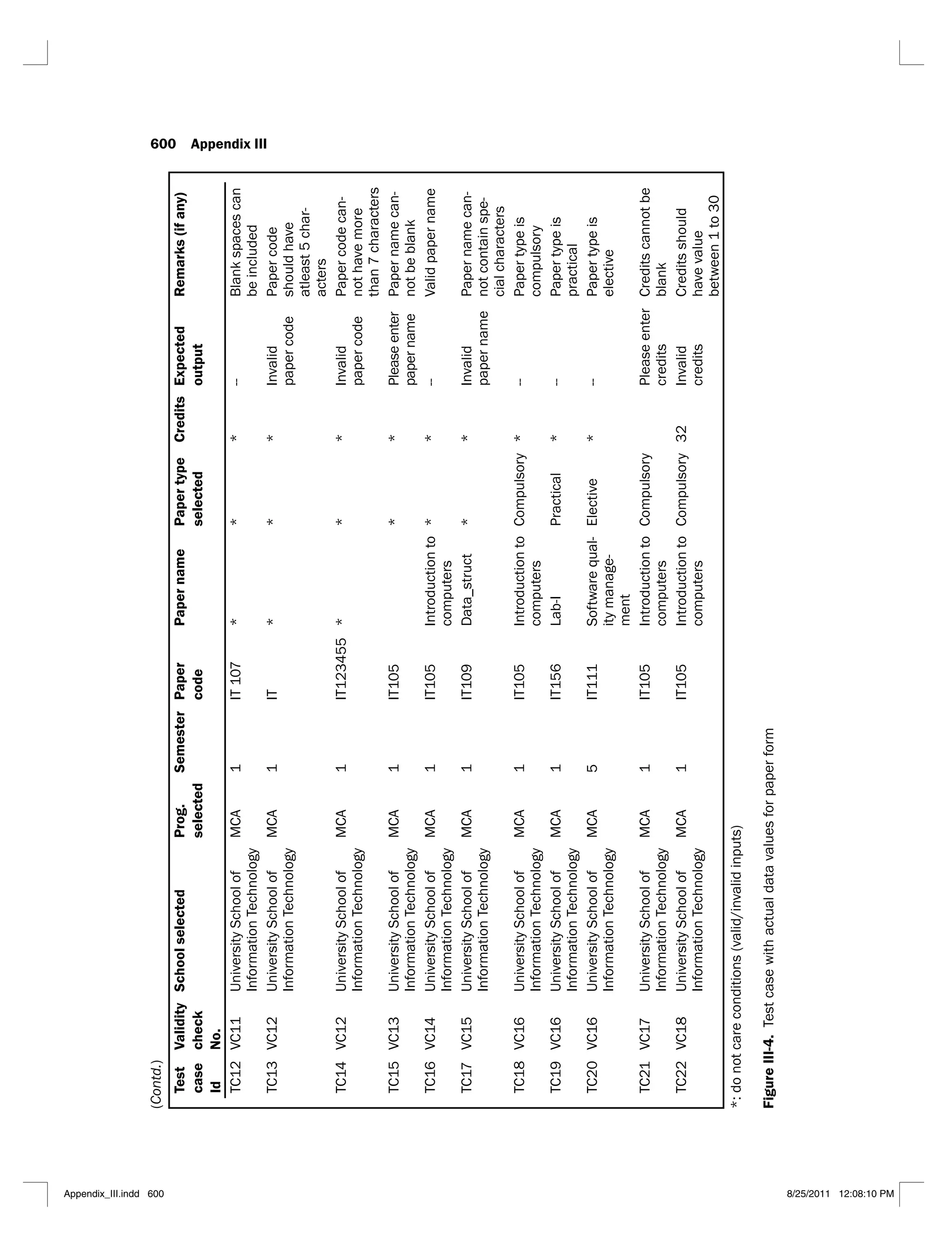
III-4 Test case with actual data values for paper form 600
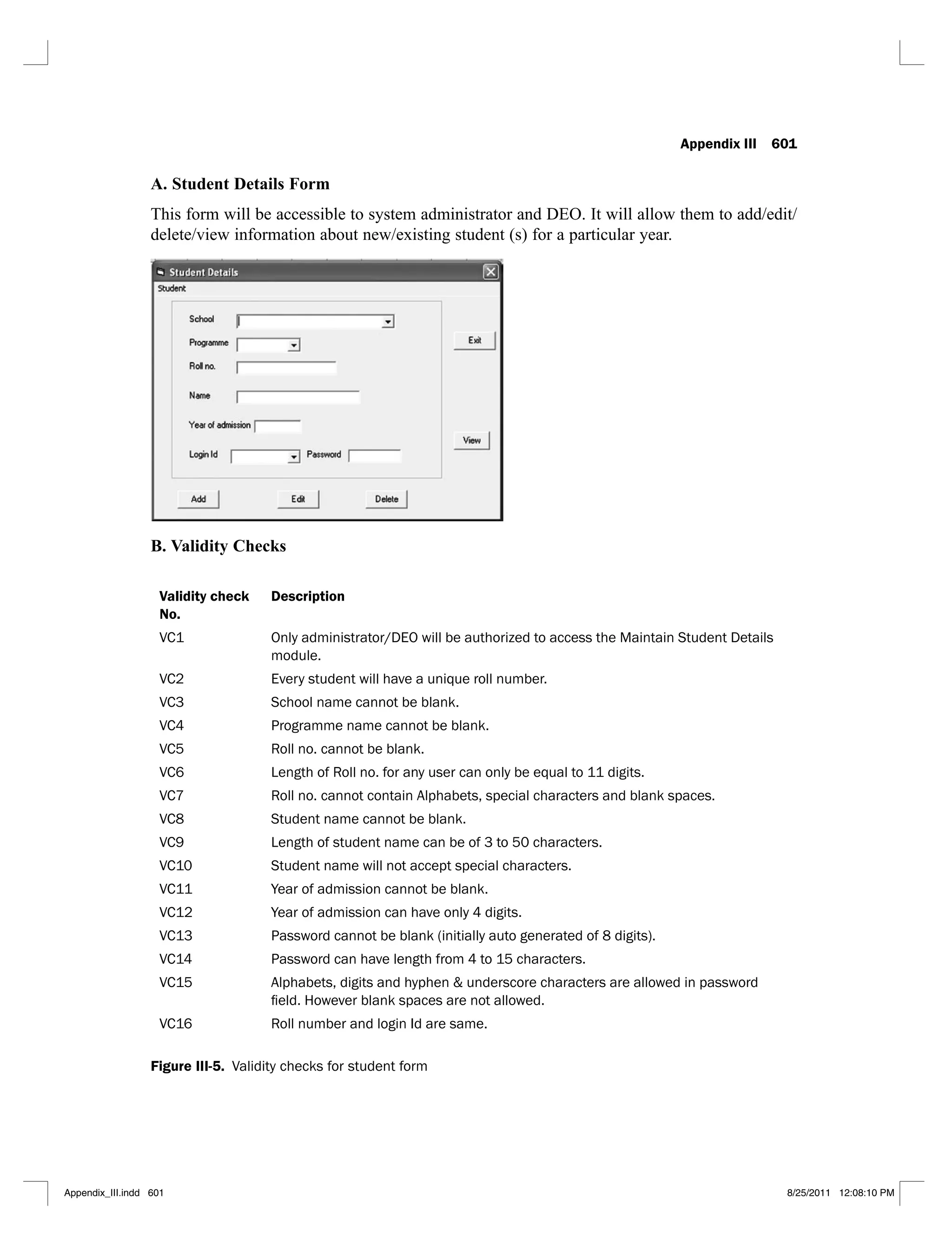
III-5 Validity checks for student form 601
III-6 Test case with actual data values for the student form 603
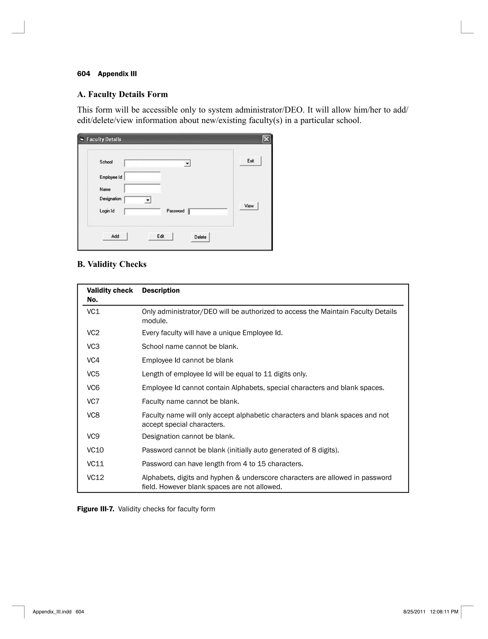
III-7 Validity checks for faculty form 604
III-8 Test case with actual data values for the faculty form 605
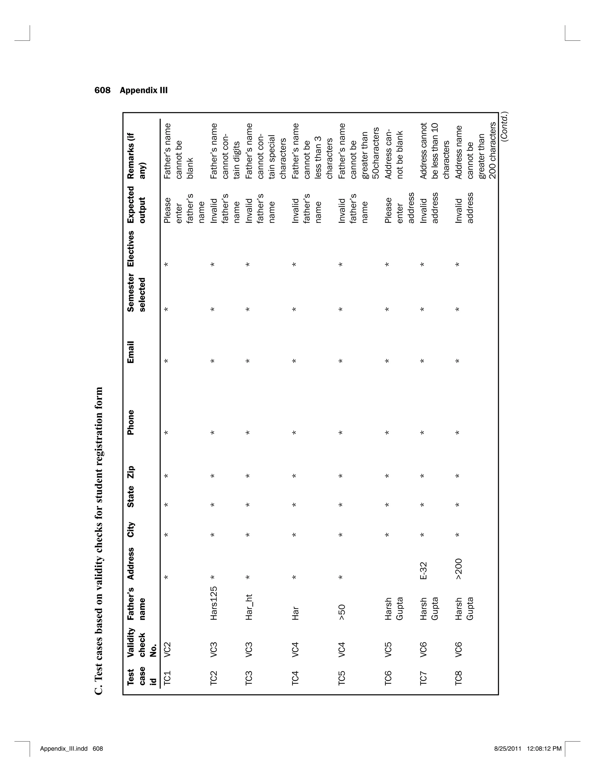
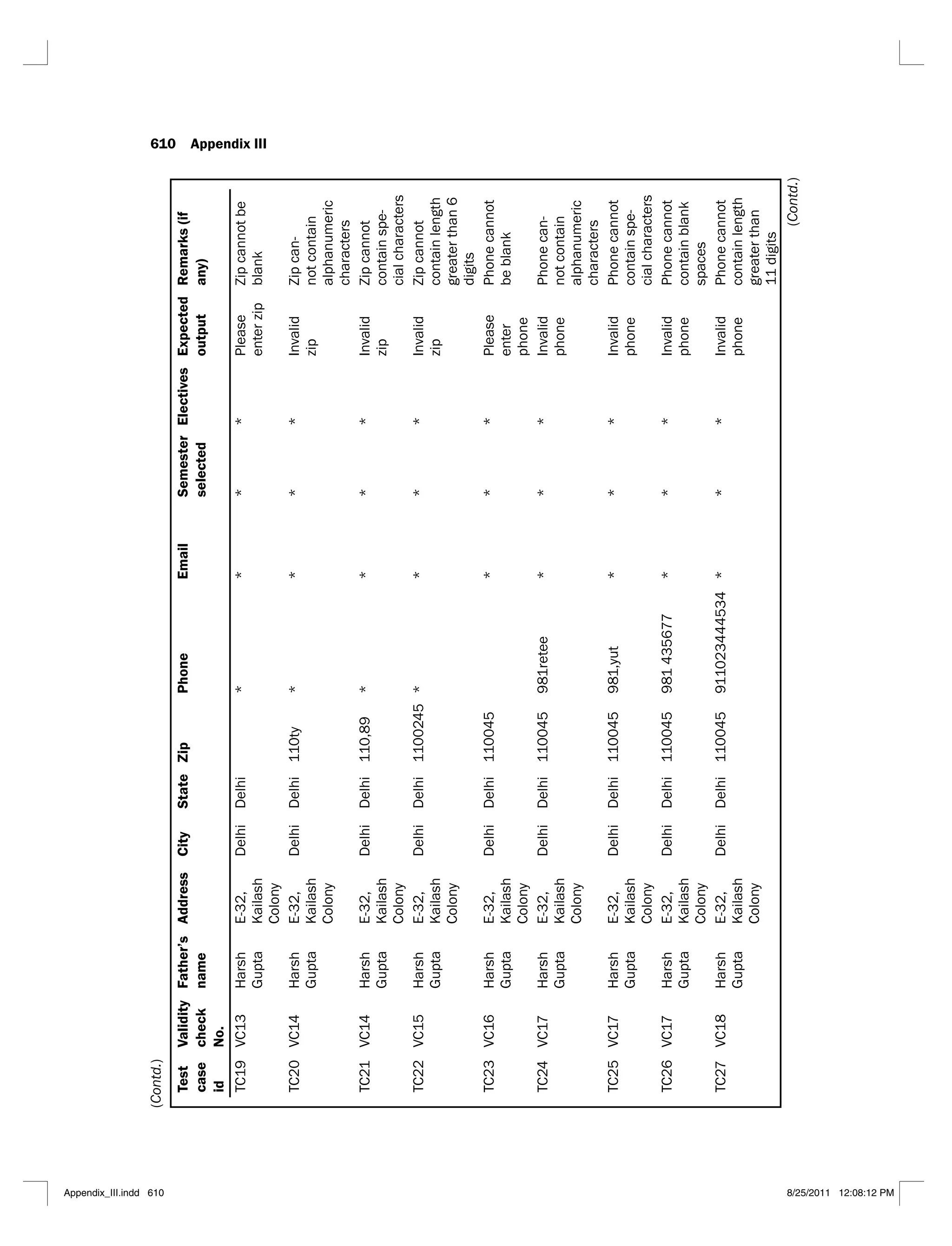
III-9 Validity checks for maintain registration details 607
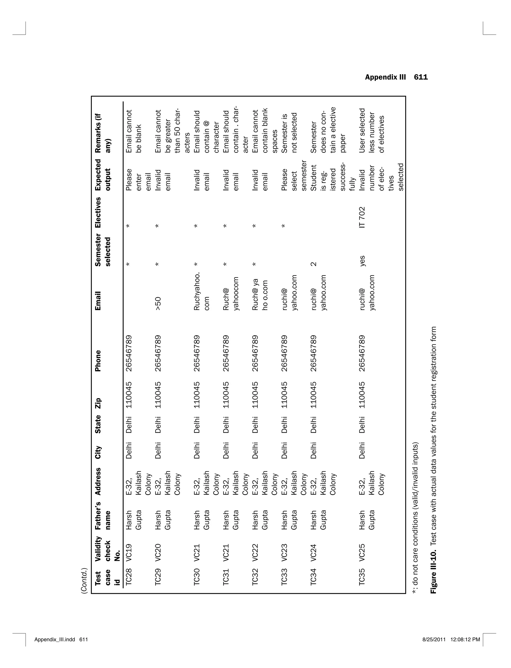
III-10 Test case with actual data values for the student registration form 611
List of Tables
1.1 Inputs and outputs of the program ‘Minimum’ 6
1.2 Some critical/typical situations of the program ‘Minimum’ 7
1.3 Possible reasons of failures for all nine cases 8
1.4 Reasons for observed output 9
1.5 Results of the modified program ‘Minimum’ 12
1.6 Persons and their roles during development and testing 16
1.7 Test case template 21
1.8 Test cases for function of Figure 1.9 25
1.9 Typical test cases where outputs are different 26
2.1 Test cases for the ‘Square’ program 38
2.2 Test cases for the program ‘Addition’ 40
2.3 Boundary value test cases to find the largest among three numbers 41
2.4 Boundary value test cases for the program determining the division of a student 41
2.5 Boundary value test cases for triangle classification program 42
2.6 Boundary value test cases for the program determining the day of the week 43
2.7 Robustness test cases for two input values x and y 44
2.8 Worst test cases for the program ‘Addition’ 45
2.9 Robust worst test cases for the program ‘Addition’ 47
2.10 Robust test cases for the program to find the largest among three numbers 48
2.11 Worst case test cases for the program to find the largest among three numbers 48
2.12 Robust test cases for the program determining the division of a student 51
2.13 Worst case test cases for the program for determining the division of a student 52
2.14 Robust test cases for the triangle classification program 55
2.15 Worst case test cases for the triangle classification program 55
2.16 Robust test cases for program for determining the day of the week 59
2.17 Worst case test cases for the program determining day of the week 59
2.18 Test cases for program ‘Square’ based on input domain 63
2.19 Test cases for the program ‘Addition’ 64
2.20 Test cases for program ‘Square’ based on output domain 65
2.21 Test cases for program ‘Addition’ based on output domain 65
2.22 Output domain test cases to find the largest among three numbers 66
2.23 Input domain test case 67
2.24 Output domain test cases 68
2.25 Input domain test cases 70
xvi List of Tables
2.26 Output domain test cases for triangle classification program 71
2.27 Input domain test cases 73
2.28 Output domain equivalence class test cases 74
2.29 Input domain equivalence class test cases 78
2.30 Decision table 81
2.31 Typical structure of a decision table 82
2.32 Decision table for triangle problem 82
2.33 Decision table 84
2.34 Test cases of the given problem 84
2.35 Limited entry decision table 85
2.36 Test cases of the given problem 86
2.37 Extended entry decision table 87
2.38 Test cases of the problem 88
2.39 Decision table 89
2.40 Test cases 90
2.41 Modified decision table 90
2.42 Test cases of the decision table given in table 2.41 92
2.43 Decision table 94
2.44 Test cases of the program day of the week 95
2.45 Decision table of rental car problem 100
2.46 Test cases of the given decision table 100
2.47 Decision table 101
3.1 Paths of undirected graph in Figure 3.1(a) 116
3.2 Paths of directed graph in Figure 3.1(b) 117
3.3 Mapping of program graph nodes and DD graph nodes 127
3.4 Mapping of program graph nodes and DD graph nodes 131
3.5 Mapping of program graph nodes and DD graph nodes 135
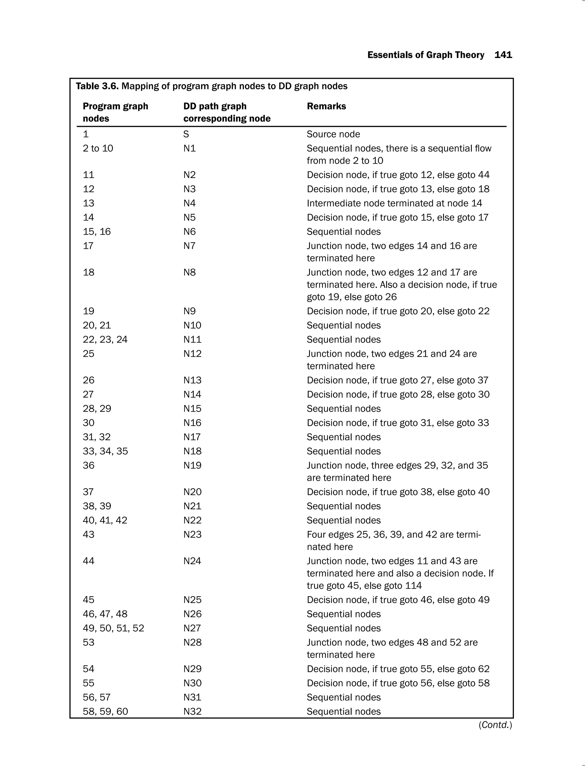
3.6 Mapping of program graph nodes to DD graph nodes 141
4.1 Test cases 168
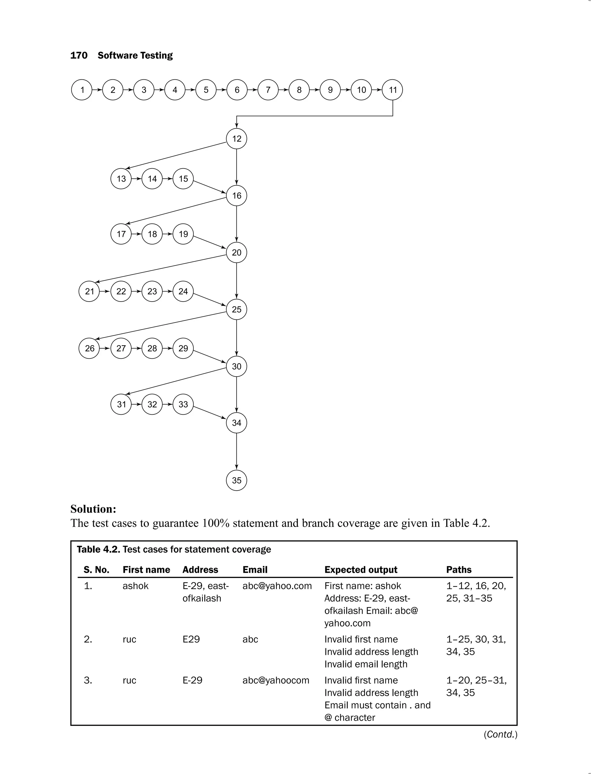
4.2 Test cases for statement coverage 170
4.3 Test cases for path coverage 171
4.4 Test cases for statement coverage 172
4.5 Test cases for path coverage 173
4.6 Test cases for all du-paths and all uses 180
4.7 Test cases for all definitions 180
4.8 All du-paths 182
4.9 Test cases for all du-paths 183
4.10 All uses paths for triangle classification problem 184
4.11 Test cases for all uses paths 185
4.12 All definitions paths for triangle classification problem 185
4.13 Test cases for all definitions paths 186
4.14 All uses paths for determination of the day of week problem 189
4.15 Test cases for all uses 192
4.16 All-definitions paths for determination of the day of week problem 195
4.17 Test cases for all-definitions 196
4.18 Test cases using program slices of program to find the largest among
three numbers 203
4.19 Test cases using program slices 207
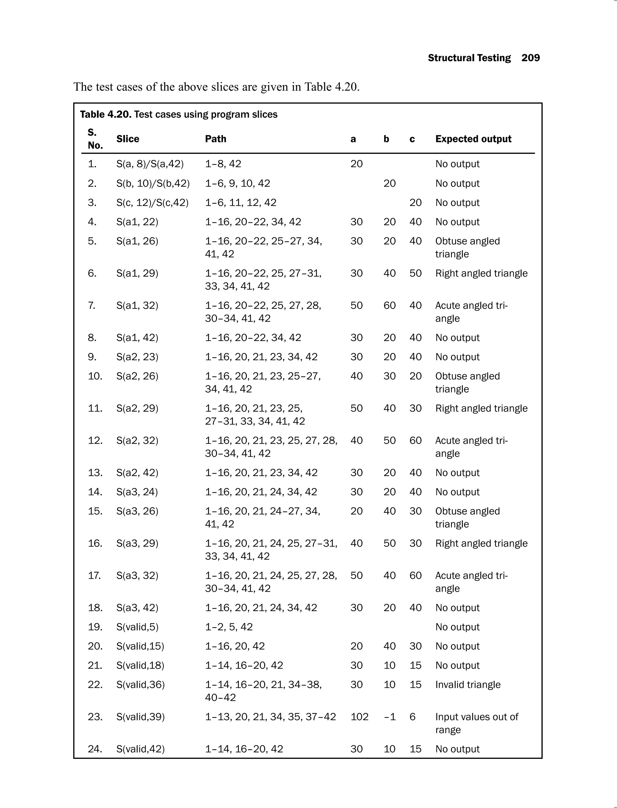
4.20 Test cases using program slices 209
4.21 Test cases using program slices 211
4.22 Mutated statements 217
4.23 Actual output of mutant M1
217
4.24 Actual output of mutant M2
217
4.25 Actual output of mutant M3
218
4.26 Actual output of mutant M4
218
4.27 Actual output of mutant M5
218
4.28 Additional test case 218
4.29 Output of added test case 218
4.30 Revised test suite 219
4.31 Test suite A 219
4.32 Test suite B 219
4.33 Mutated lines 219
4.34 Actual output of M1
(A) 220
4.35 Actual output of M2
(A) 220
4.36 Actual output of M3
(A) 220
4.37 Actual output of M4
(A) 220
4.38 Actual output of M5
(A) 221
4.39 Actual output of M1
(B) 221
4.40 Actual output of M2
(B) 221
4.41 Actual output of M3
(B) 222
4.42 Actual output of M4
(B) 222
4.43 Actual output of M5
(B) 222
4.44 Additional test case 222
4.45 Revised test suite B 223
5.1 Comparison of verification methods 232
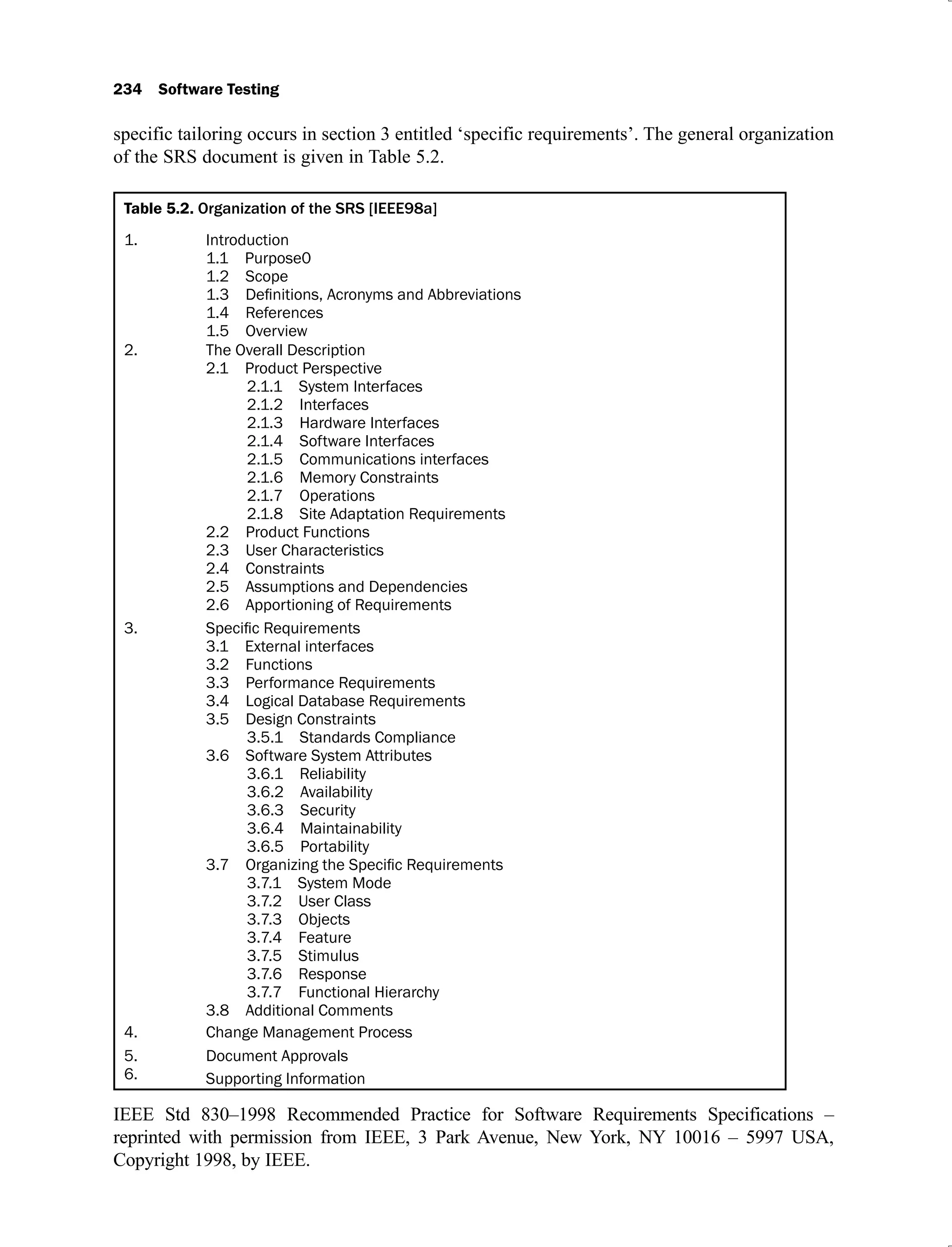
5.2 Organization of the SRS [IEEE98a] 234
5.3 Checklist for the SRS document 236
5.4 Checklist for the SDD Document 239
5.5 Source code reviews checklist 242
5.6 User Documentation checklist 244
6.1 Jacobson’s use case template 290
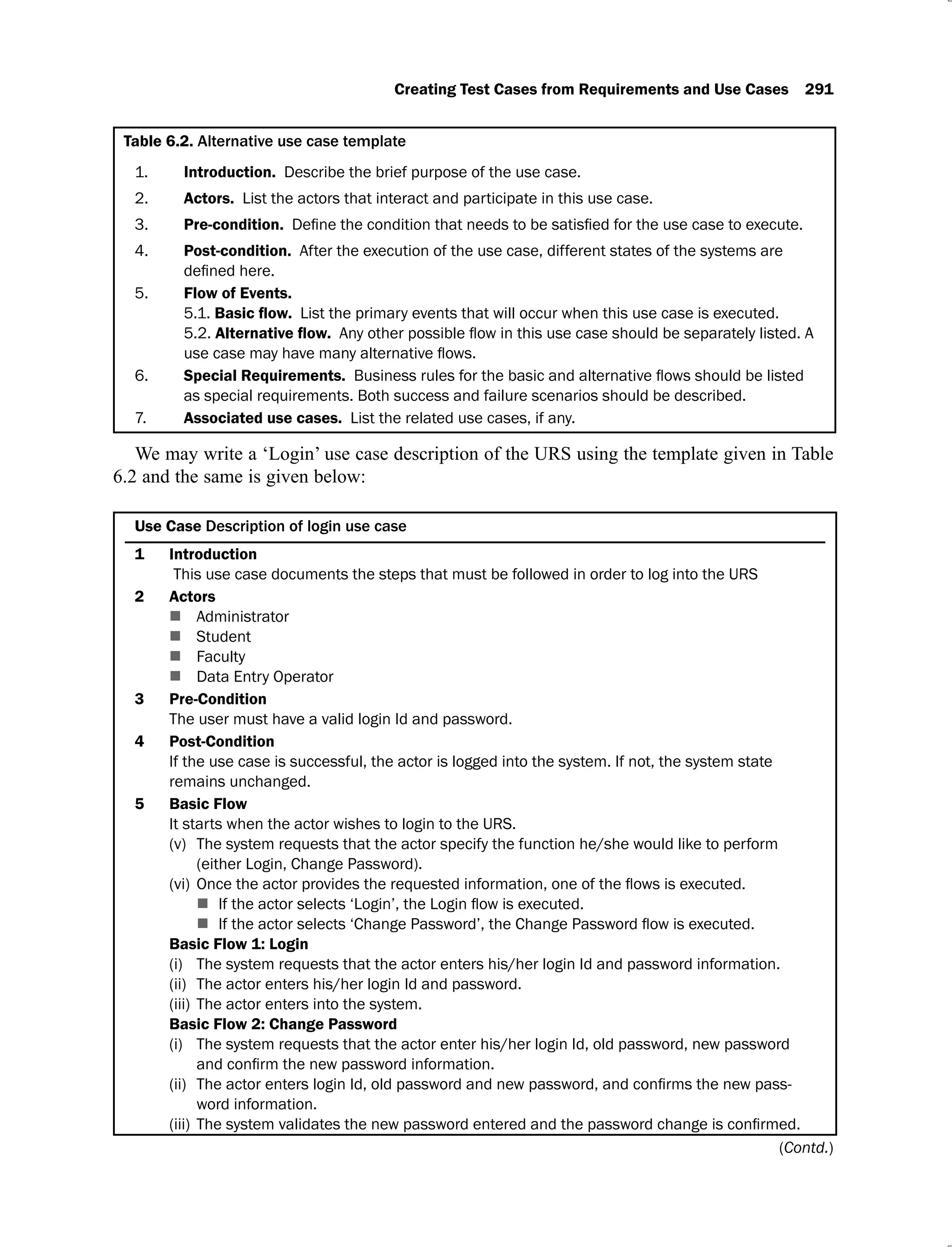
6.2 Alternative use case template 291
6.3 Scenario matrix for the flow of events shown in Figure 6.3 294
6.4 Scenario matrix for the login use case 295
6.5 A typical test case matrix 296
6.6 Test case matrix for the login use case 297
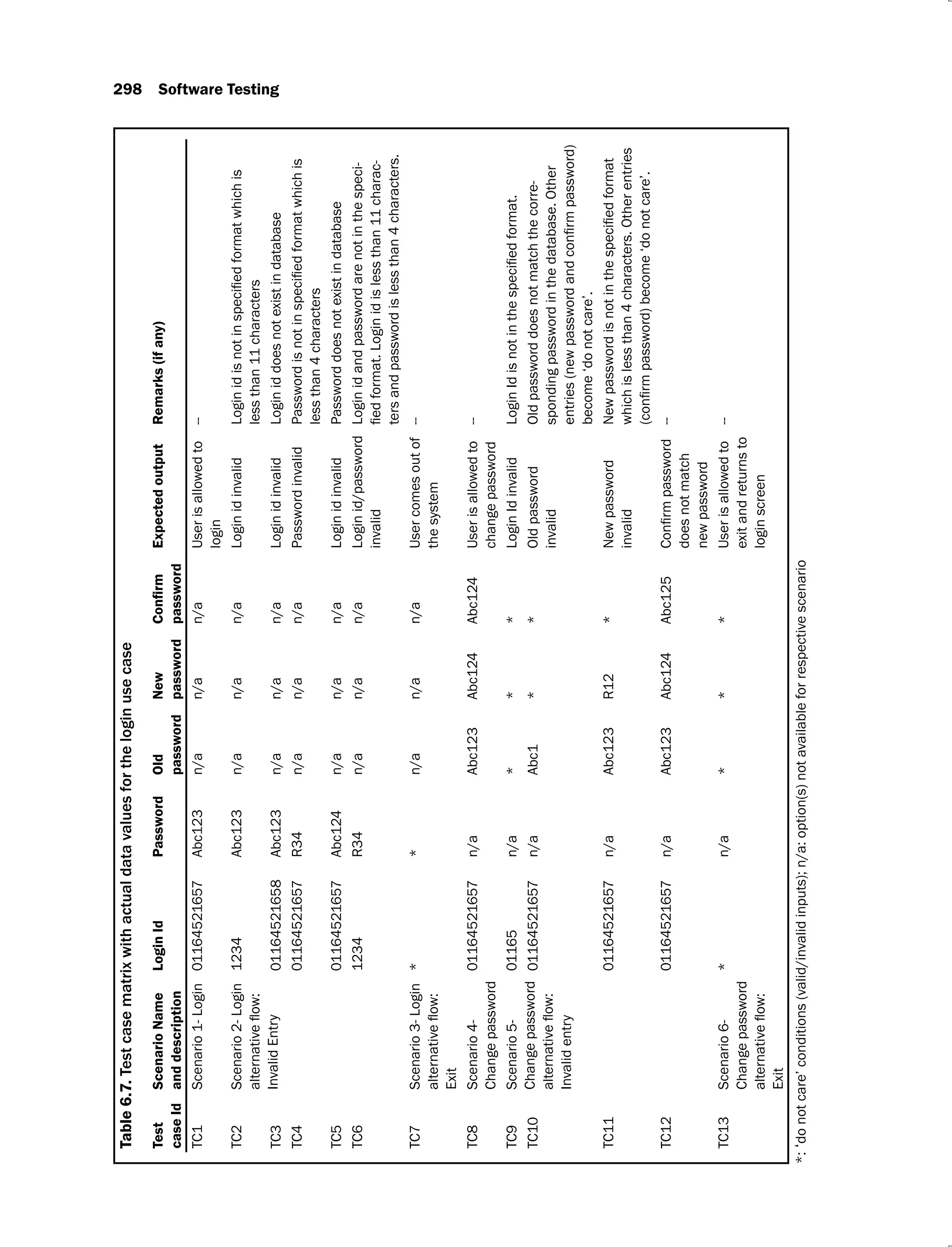
6.7 Test case matrix with actual data values for the login use case 298
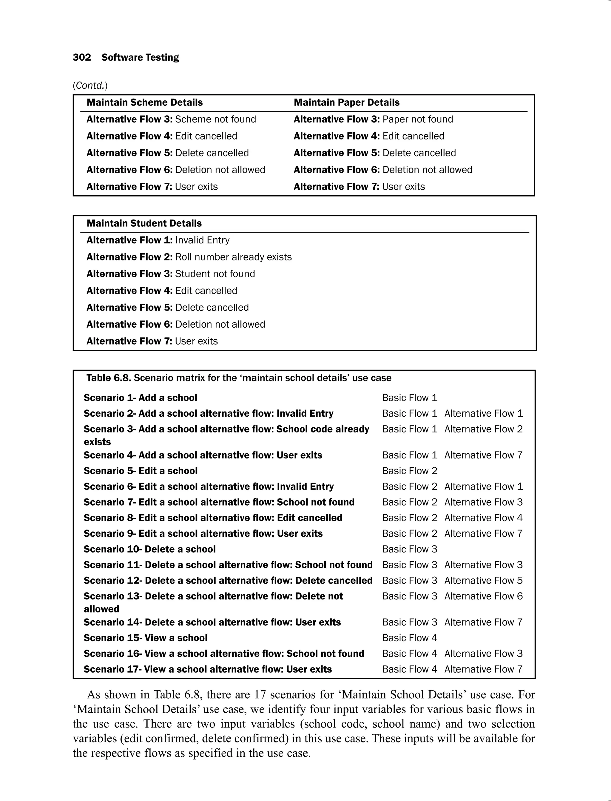
6.8 Scenario matrix for the ‘maintain school details’ use case 302
6.9 Test case matrix for the ‘maintain school details’ use case 303
6.10 Test case matrix with actual data values for the ‘maintain school’ use case 305
6.11 Scenario matrix for the ‘maintain programme details’ use case 308
List of Tables xvii
xviii List of Tables
6.12 Test case matrix for the ‘maintain programme details’ use case 309
6.13 Test case matrix with actual data values for the programme use case 313
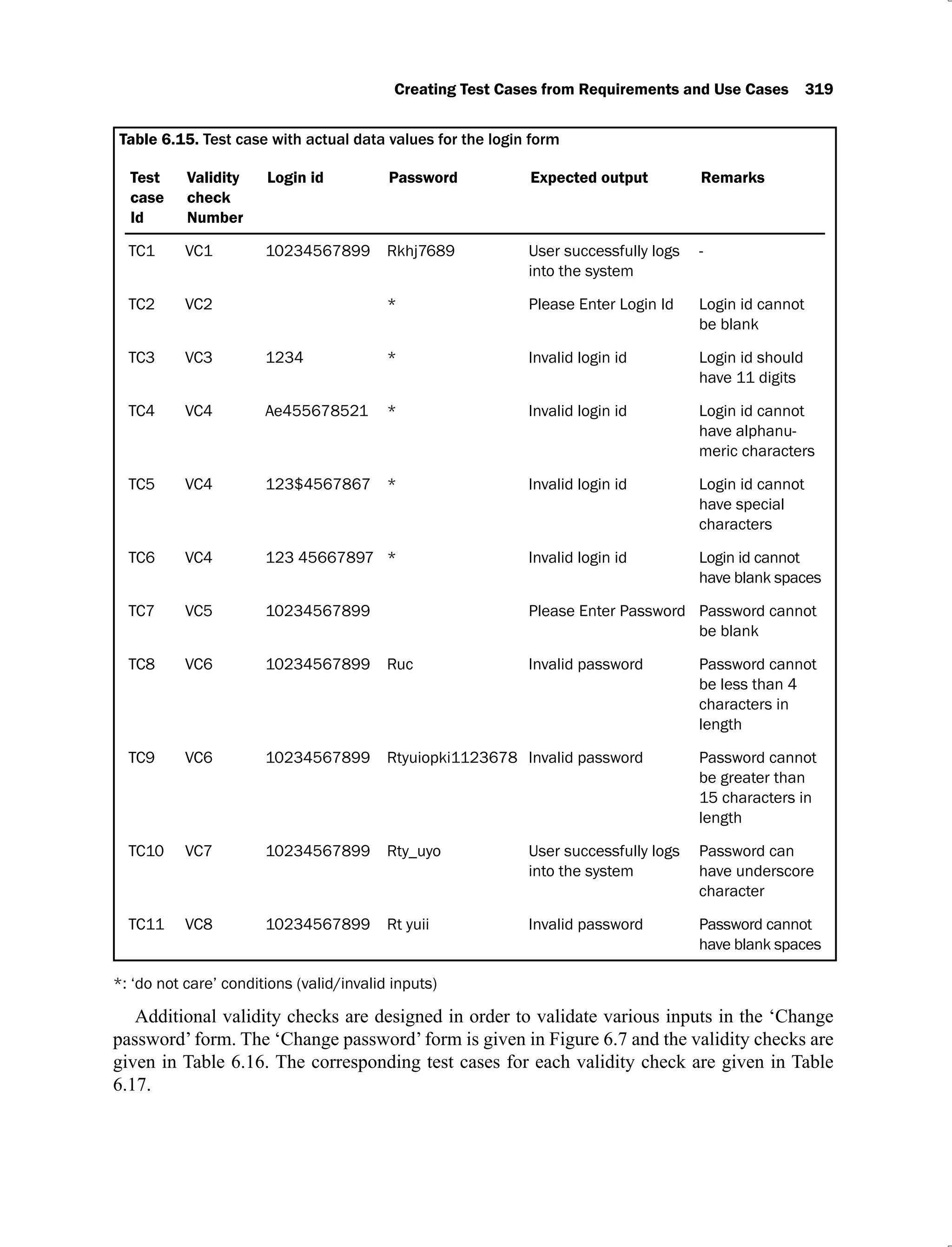
6.14 Validity checks for login form 318
6.15 Test case with actual data values for the login form 319
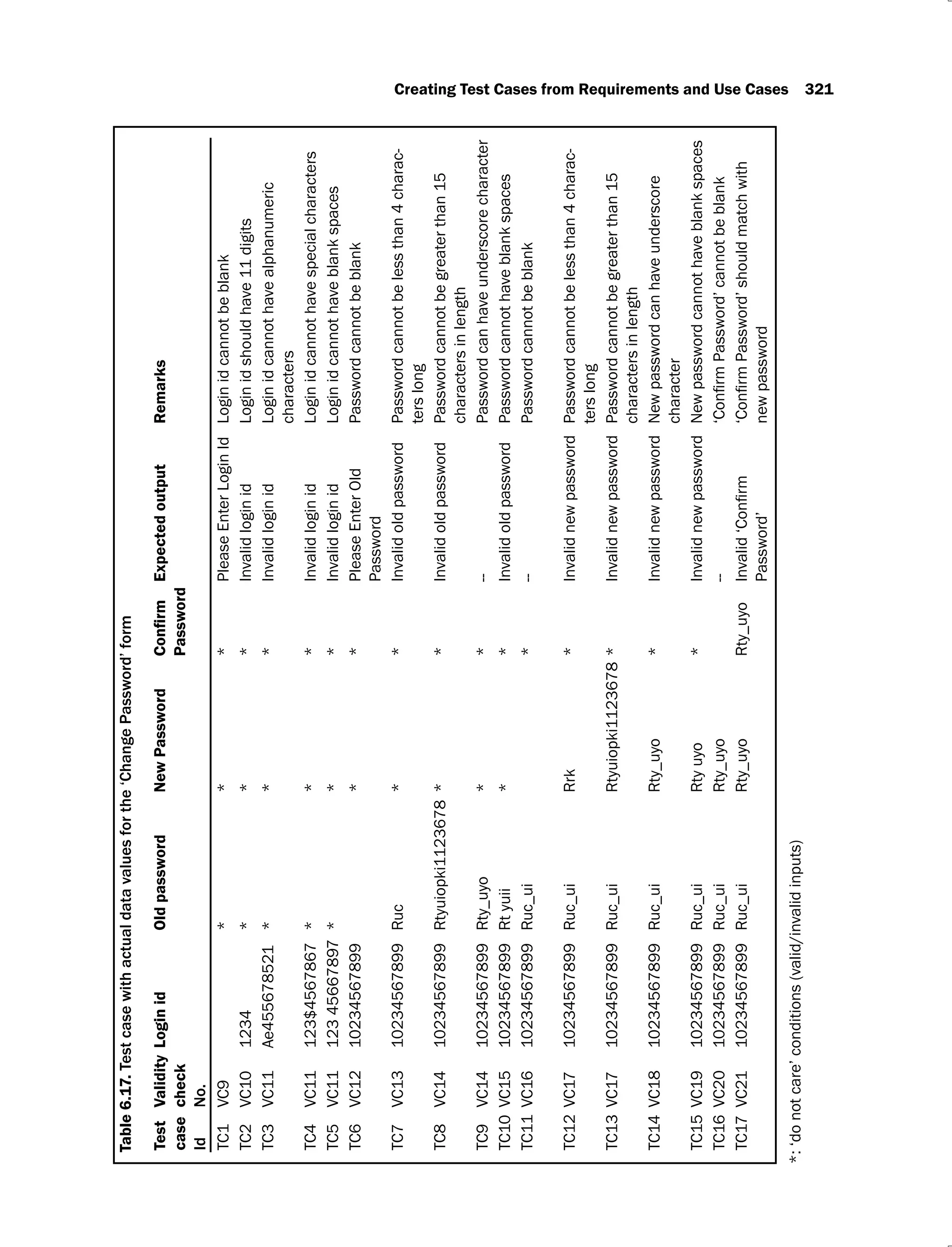
6.16 Validity checks for change password form 320
6.17 Test case with actual data values for the ‘Change Password’ form 321
6.18 Validity checks for school form 323
6.19 Test case with actual data values for the school form 323
6.20 Validity checks for program form 324
6.21 Test case with actual data values for the program form 325
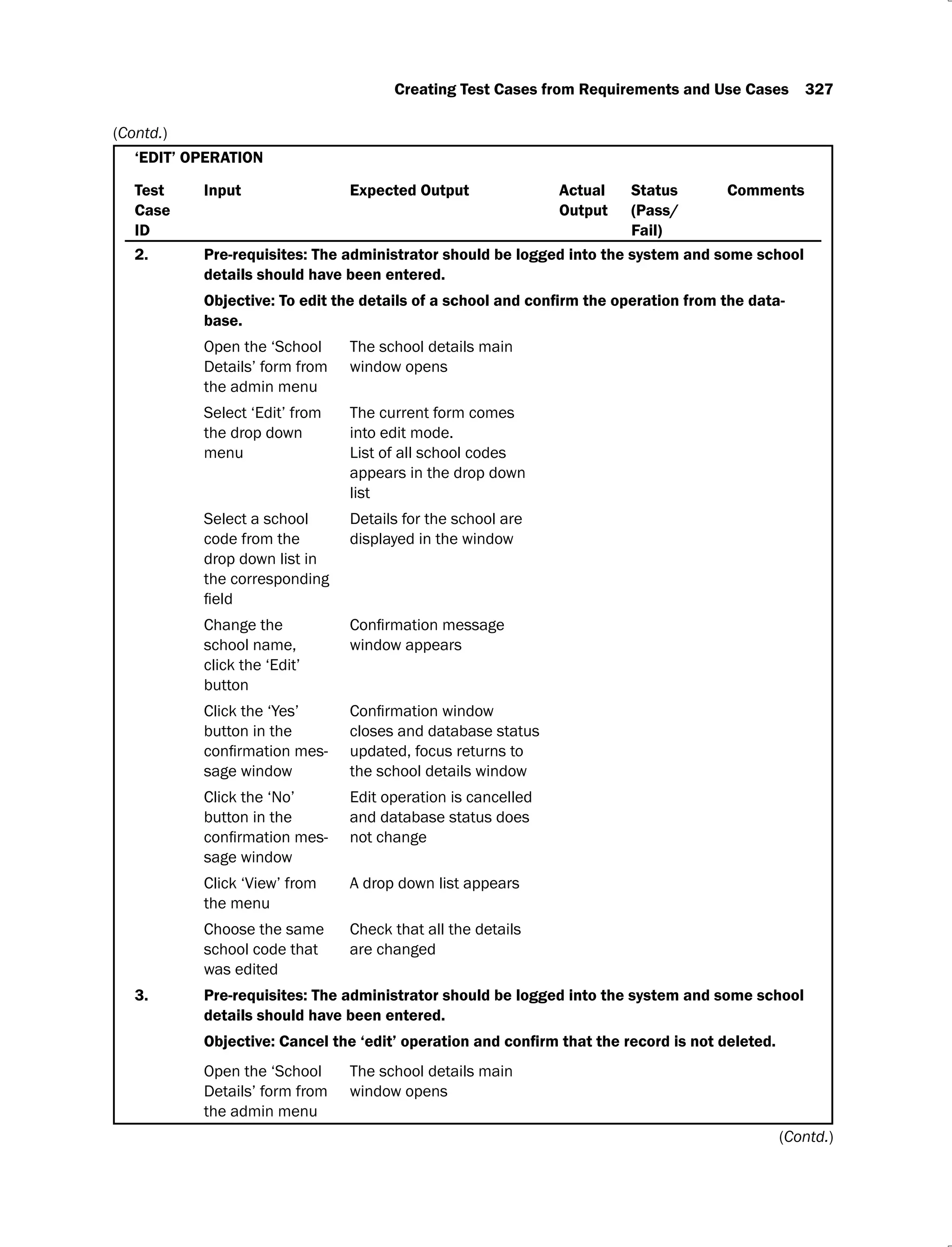
6.22 Operations of ‘school details’ form 326
7.1 Comparison of regression and development testing 336
7.2 Test suite for program given in Figure 7.2 338
7.3 Risk analysis table 342
7.4 Risk analysis table of ‘University Registration System’ 343
7.5 Variables used by ‘modification’ algorithm 347
7.6 Test cases with execution history 348
7.7 Test cases with number of matches found 349
7.8 Test cases in decreasing order of number of modified lines covered 350
7.9 Test cases in descending order of number of matches found (iteration 2) 350
7.10 Test cases in descending order of number of matches found (iteration 3) 351
7.11 Test cases in descending order of number of matches found (iteration 4) 351
7.12 Test cases in descending order of number of matches found (iteration 5) 351
7.13 Variables used by ‘deletion’ algorithm 352
7.14 Test cases with execution history 352
7.15 Modified execution history after deleting line numbers 4, 7 and 15 353
7.16 Redundant test cases 354
7.17 Modified table after removing T1 and T5 355
7.18 Test cases with modified lines 355
7.19 Test cases in descending order of number of modified lines covered 355
7.20 Test cases in descending order of number of modified lines
covered (iteration 2) 355
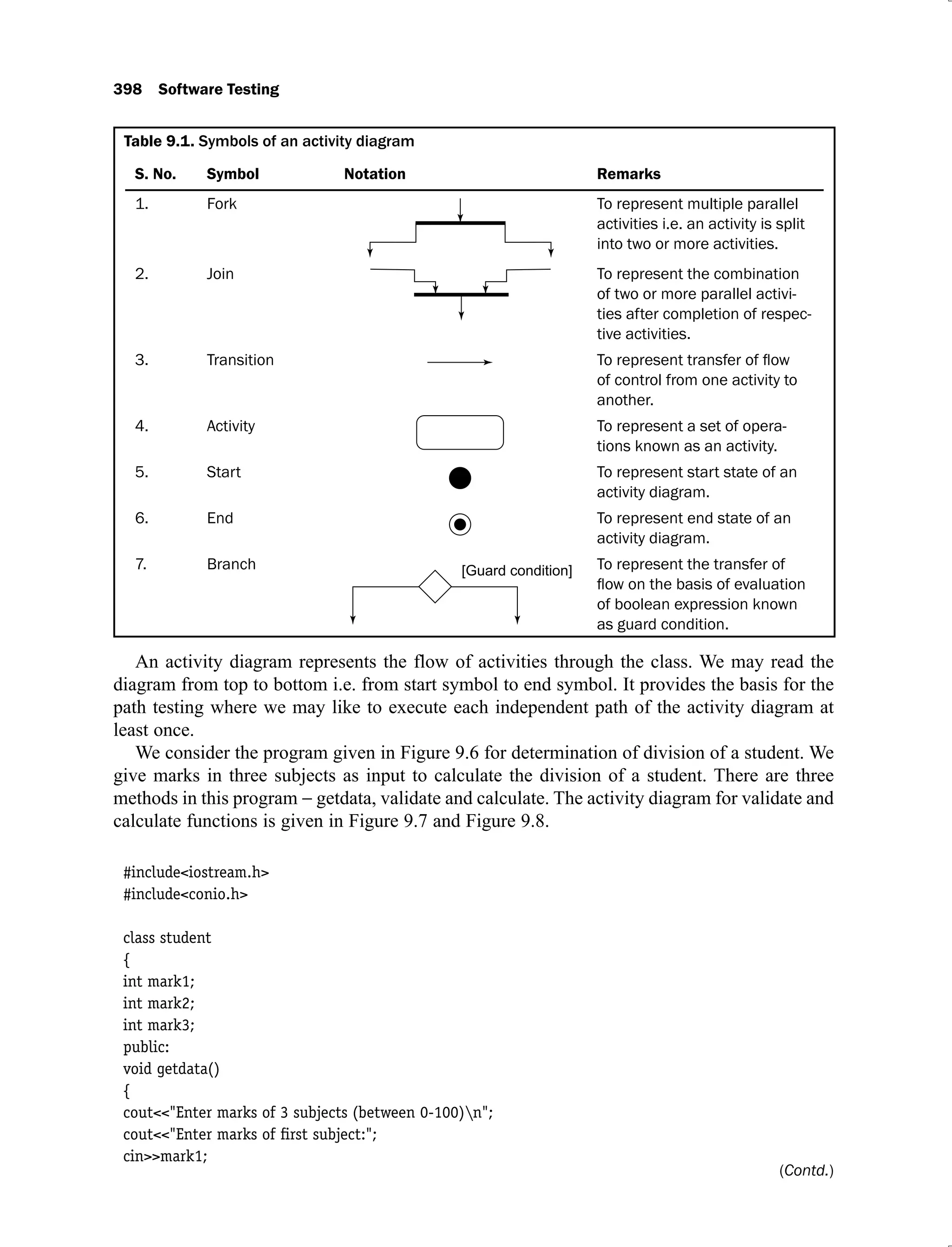
9.1 Symbols of an activity diagram 398
9.2 Test cases for validate function 401
9.3 Test cases for calculate function 402
9.4 Test cases of activity diagram in Figure 9.10 403
9.5 Test cases of activity diagram in Figure 9.11 404
9.6 Terminologies used in state chart diagram 405
9.7 State transition table for stack class 408
9.8 Test cases for class stack 409
9.9 Illegal test case for class stack 409
9.10 Test cases of withdrawal from ATM 411
9.11 Test cases of function push() 413
9.12 Test cases of function pop() 414
9.13 Test cases for function withdraw() 414
10.1 Coupling metrics 424
List of Tables xix
10.2 Cohesion metrics 425
10.3 Inheritance metrics 425
10.4 Size metrics 426
10.5 Time-based failure specification 427
10.6 Failure-based failure specification 428
10.7 Distribution of faults and faulty classes at high, medium and low
severity levels 438
10.8 Descriptive statistics for metrics 438
10.9 Correlations among metrics 439
10.10 High severity faults model statistics 439
10.11 Medium severity faults model statistics 440
10.12 Low severity faults model statistics 440
10.13 Ungraded severity faults model statistics 440
10.14 Confusion matrix 440
10.15 Results of 10-cross validation of models 441
10.16 ANN summary 443
10.17 Rotated principal components 444
10.18 Validation results of ANN model 445
10.19 Analysis of model evaluation accuracy 445
11.1 Comparison of client/server and web based applications 454
11.2 Sample functional test cases of order process of an online shopping
web application 457
11.3 Navigation testing test cases for online shopping website 459
11.4 Test cases of registration form of an online shopping web application 460
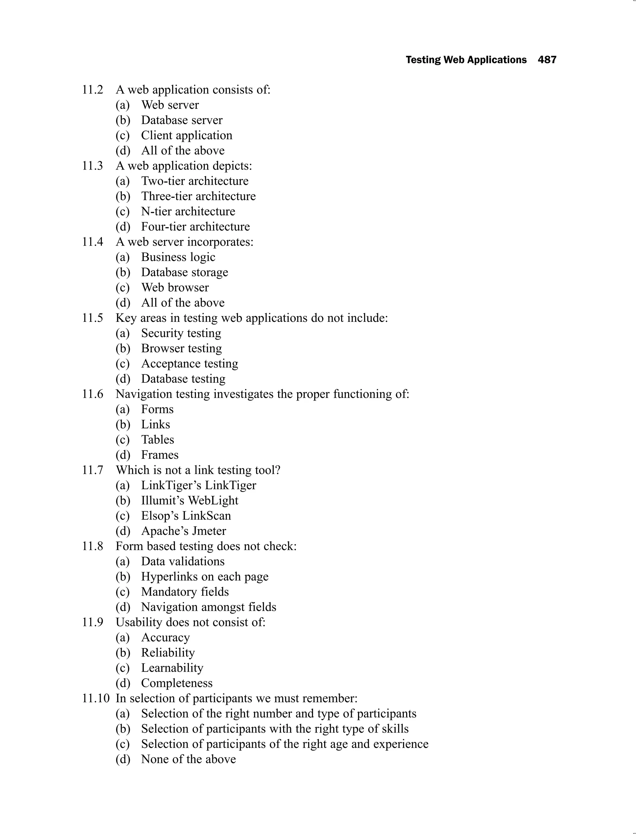
11.5 Checklist for testing user interfaces 461
11.6 Web application usability attributes 463
11.7 Browser’s compatibility matrix 470
11.8 Configuration and compatibility testing checklist 471
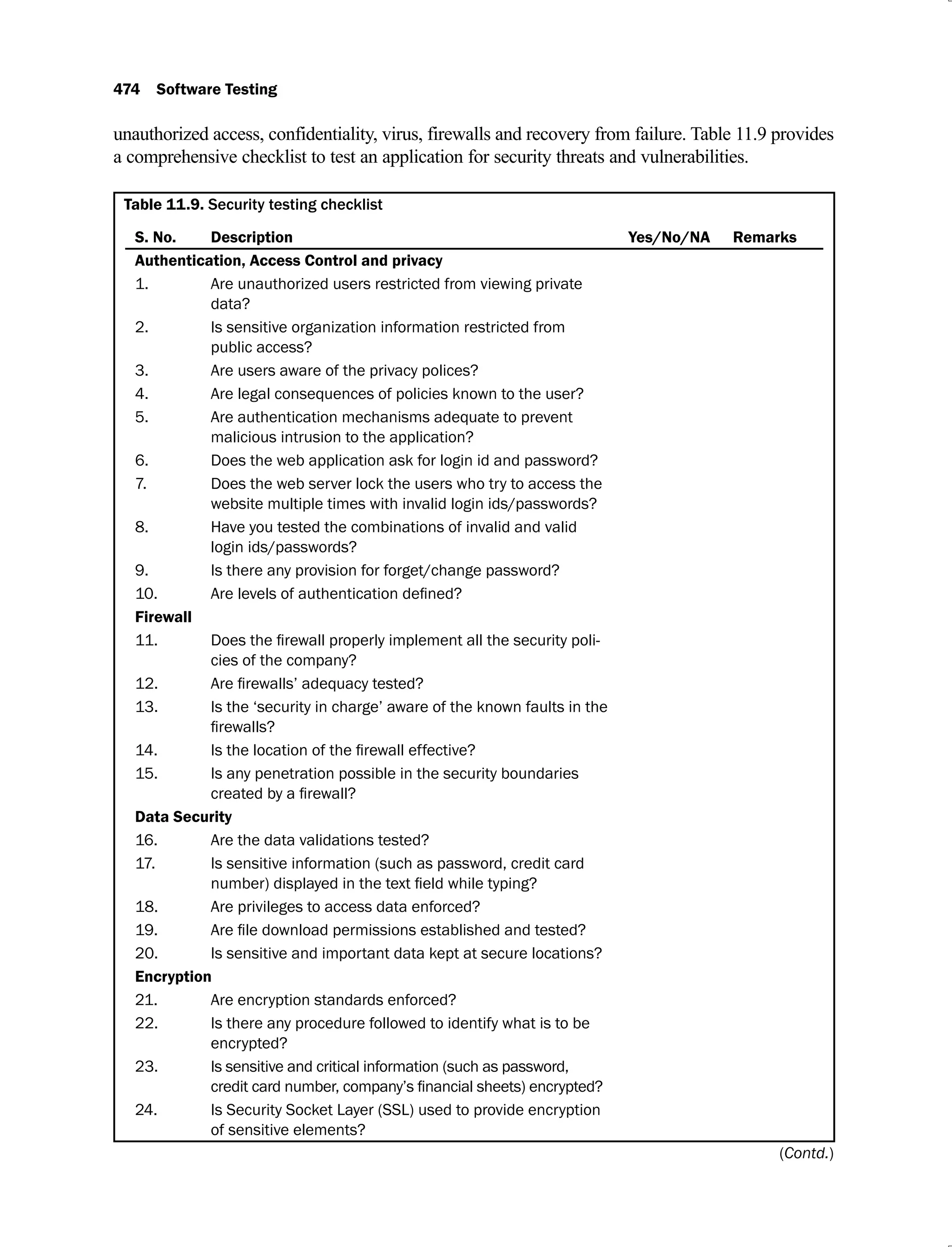
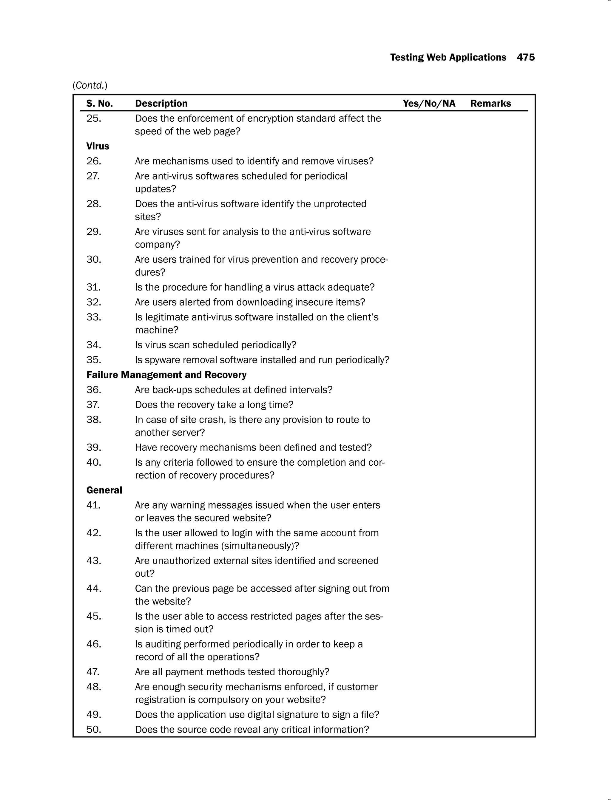
11.9 Security testing checklist 474
11.10 Load testing metrics 477
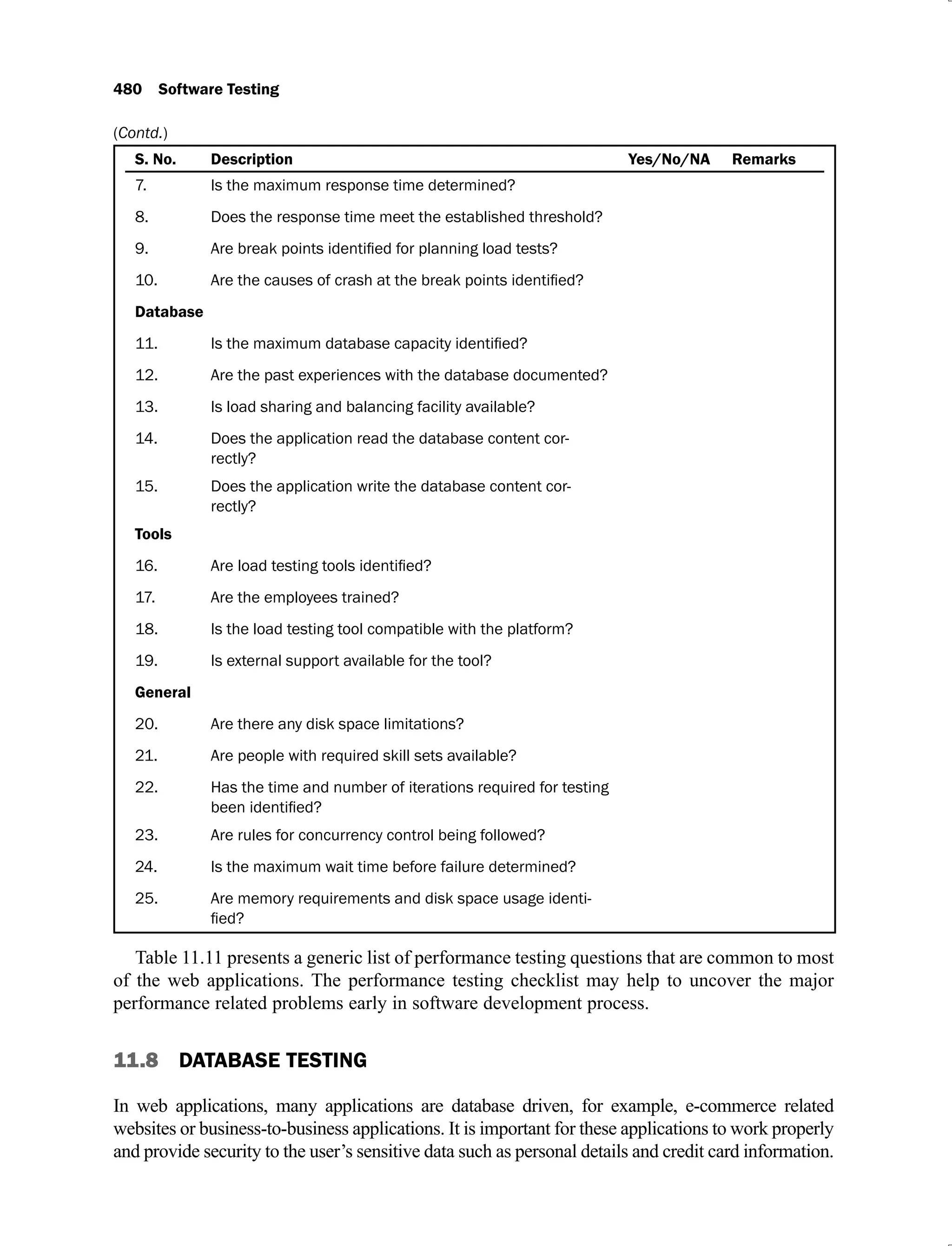
11.11 Performance testing checklist 479
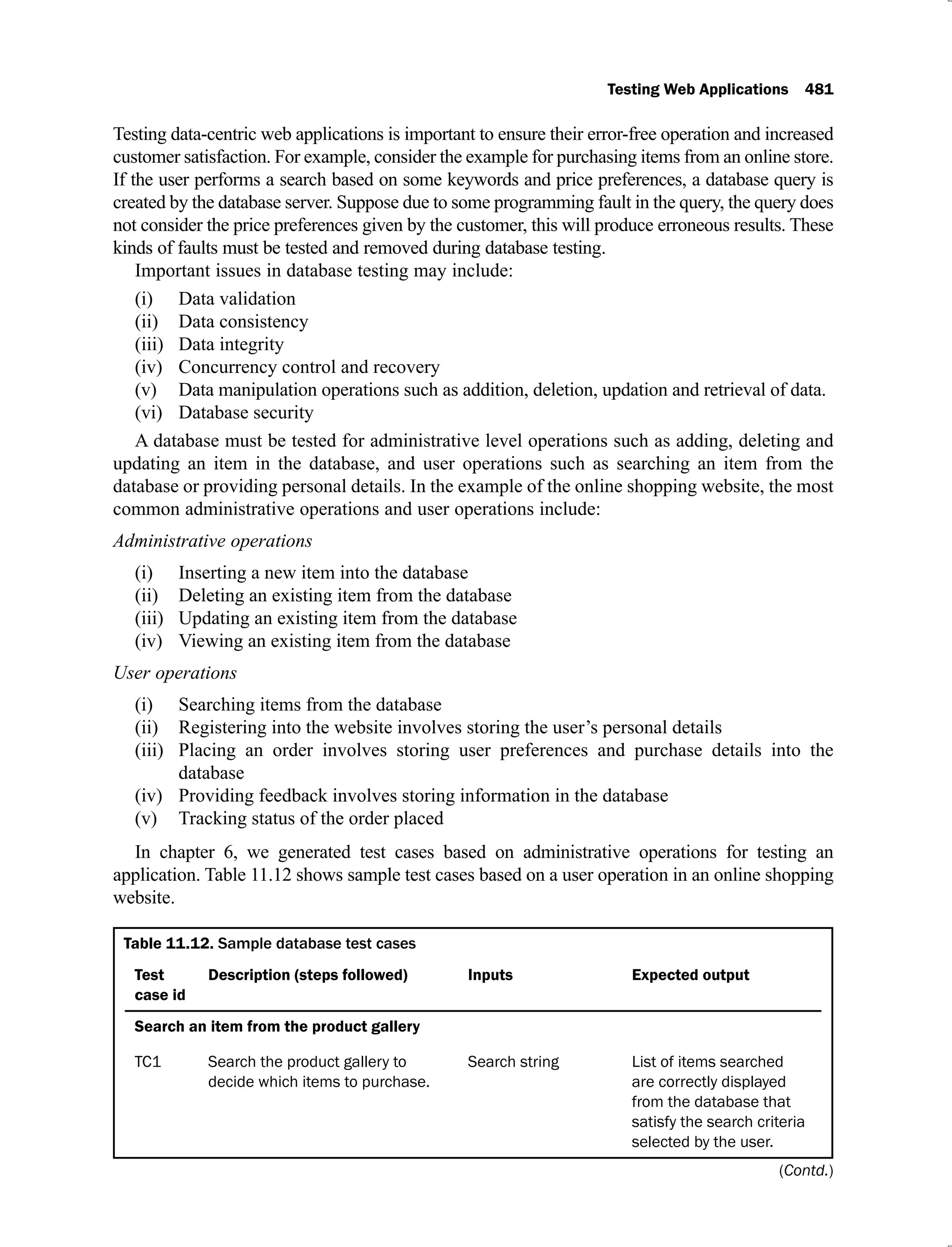
11.12 Sample database test cases 481
11.13 Web metrics 485
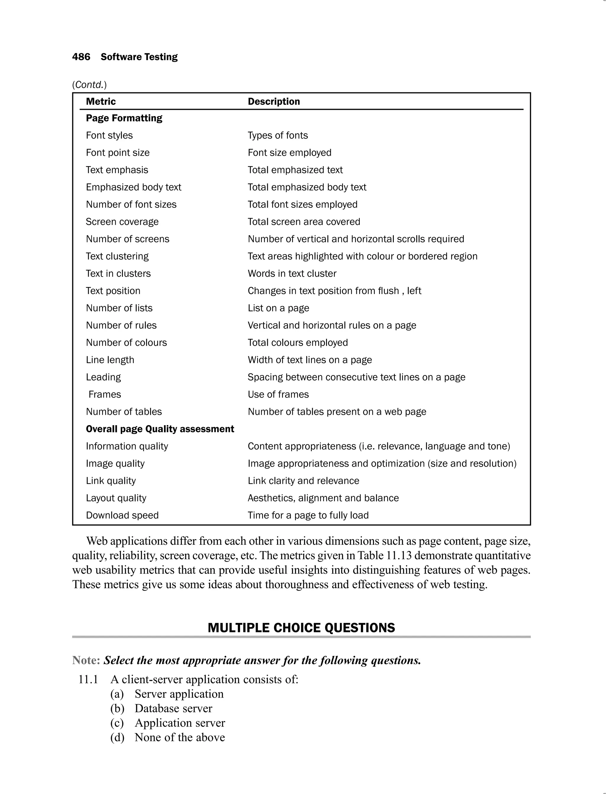
12.1 Constraints and values of paths (feasible/not feasible) of program given
in Figure 12.1 499
12.2 Examples of one point crossover operator 503
12.3 Examples of two point crossover operator 504
12.4 Chromosomes with fitness values for initial population 505
12.5 Automated test data generation tools 511
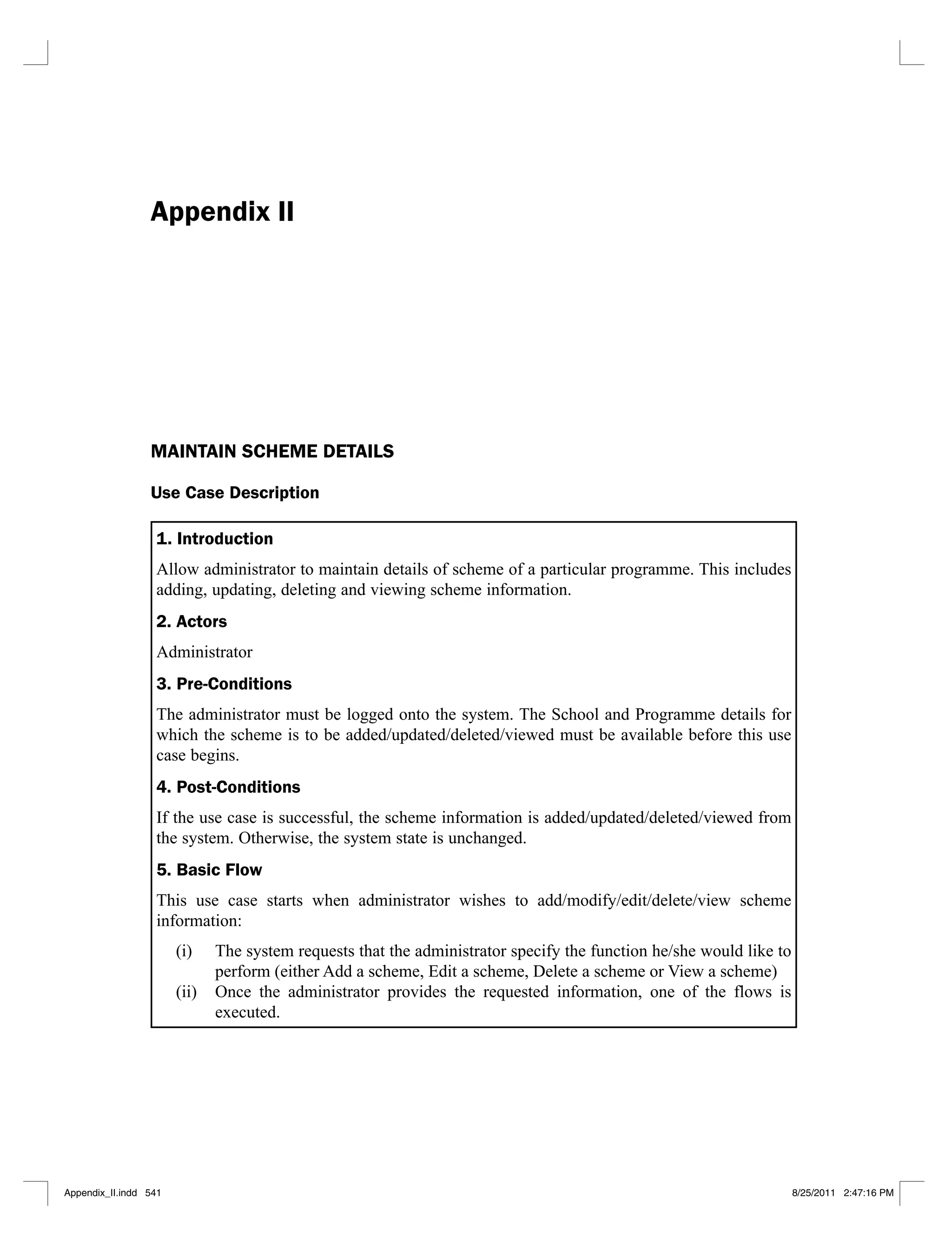
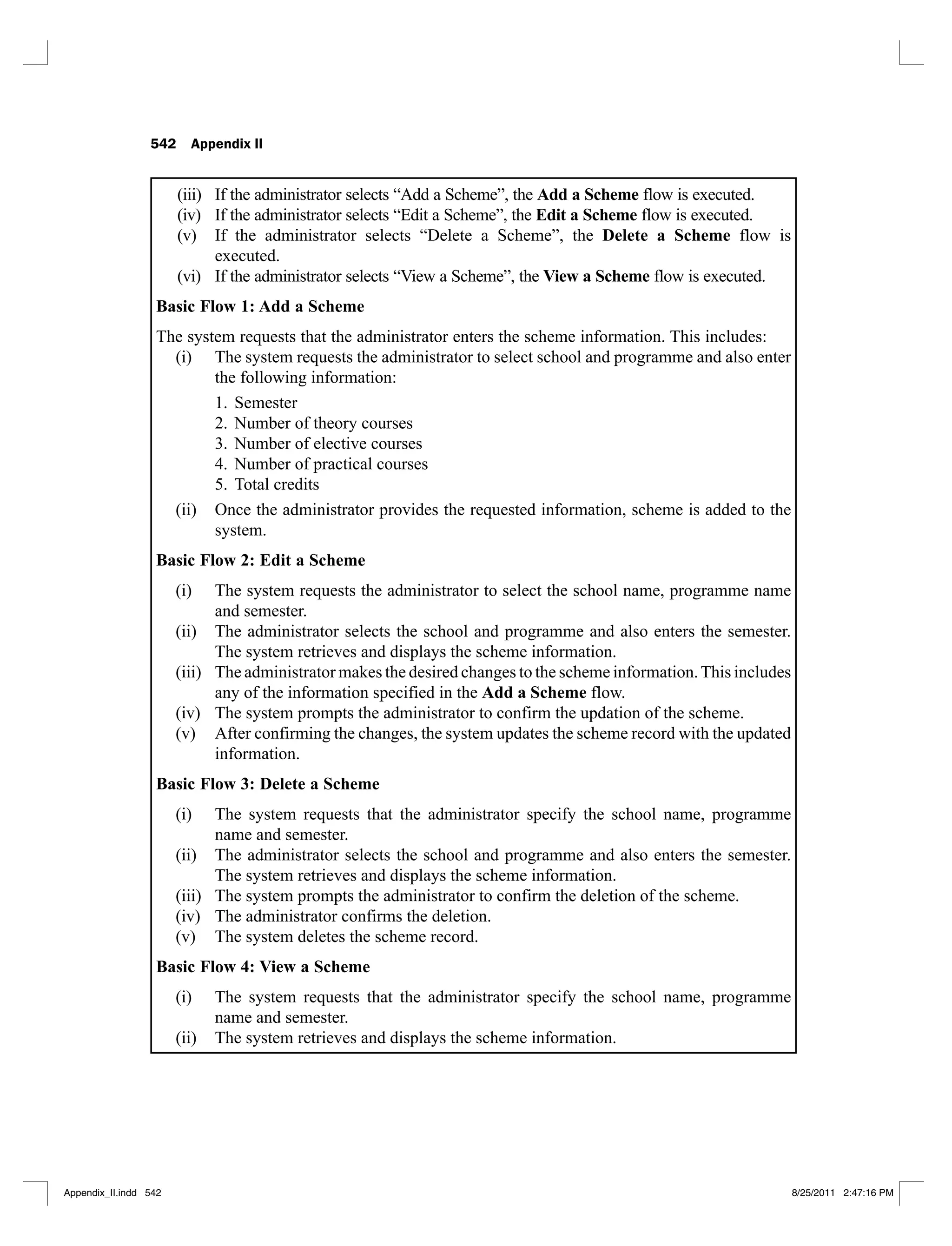
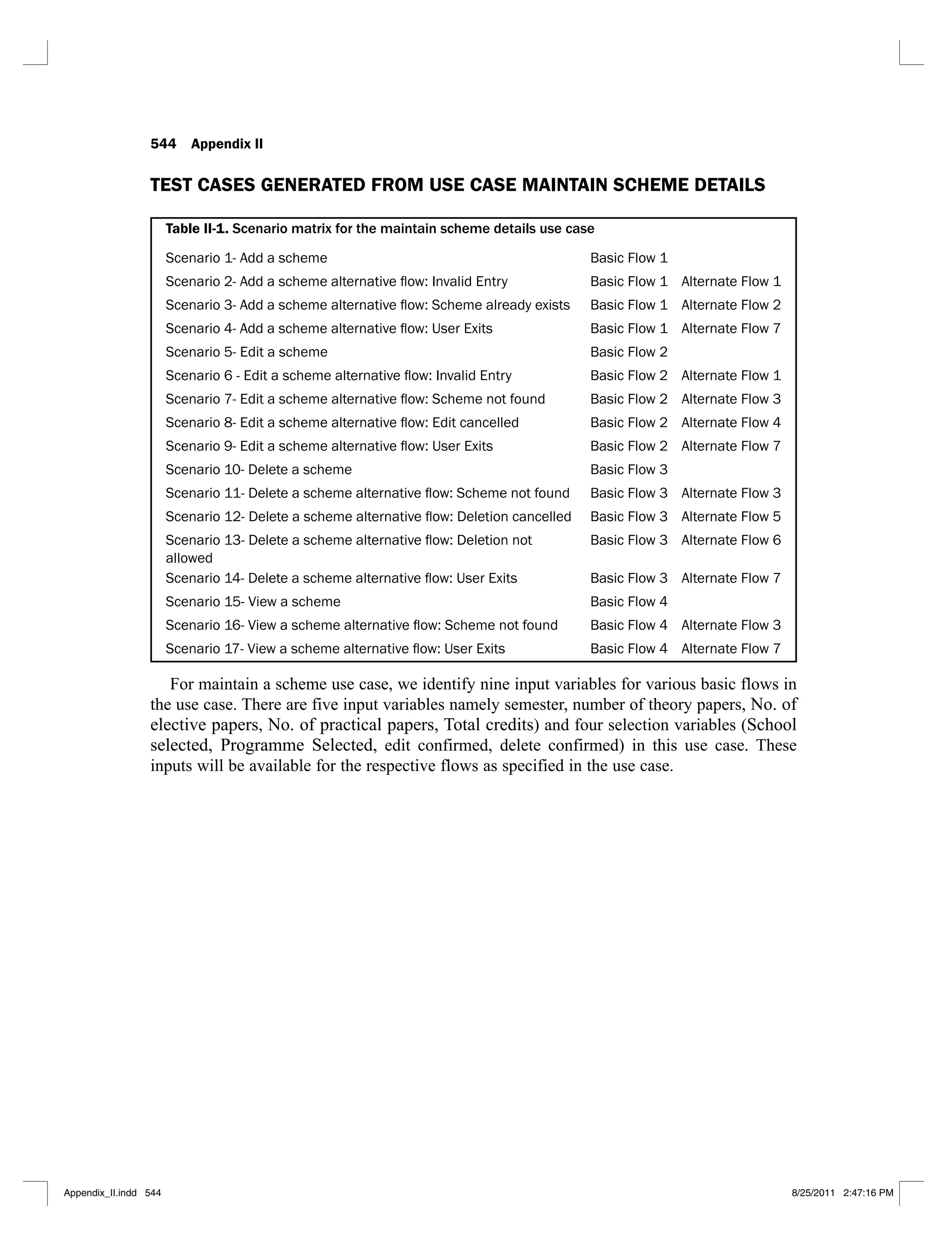
II-1 Scenario matrix for the maintain scheme details use case 544
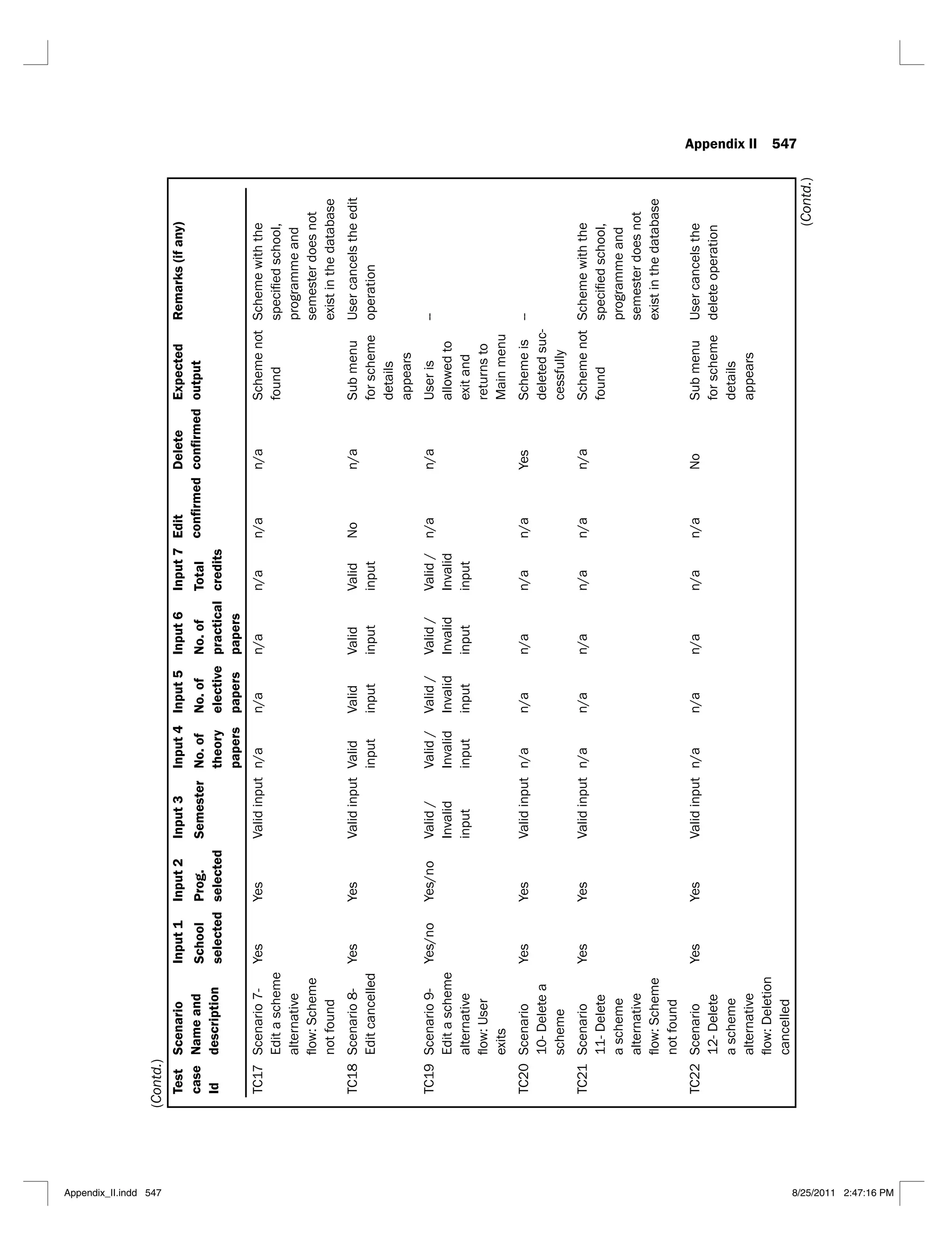
II-2 Test case matrix for the maintain scheme details use case 545
II-3 Test case matrix with actual data values for the maintain scheme details
use case 549
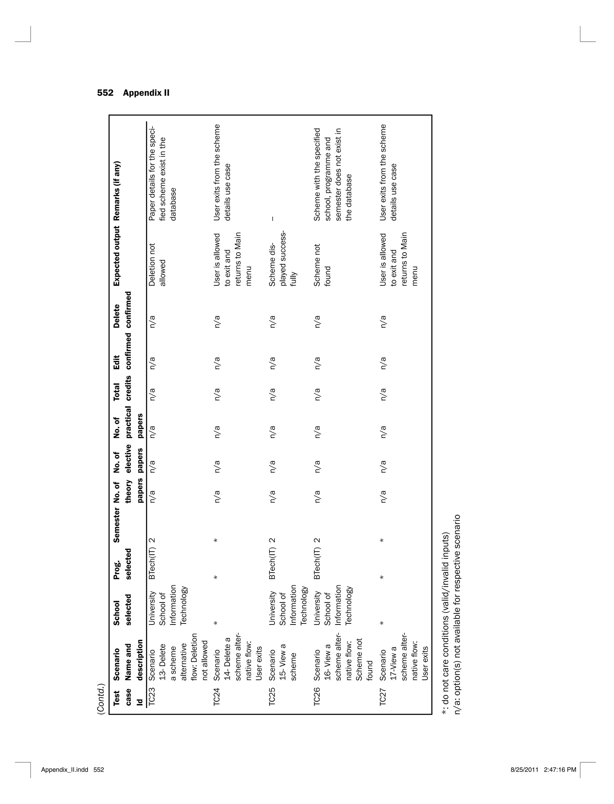
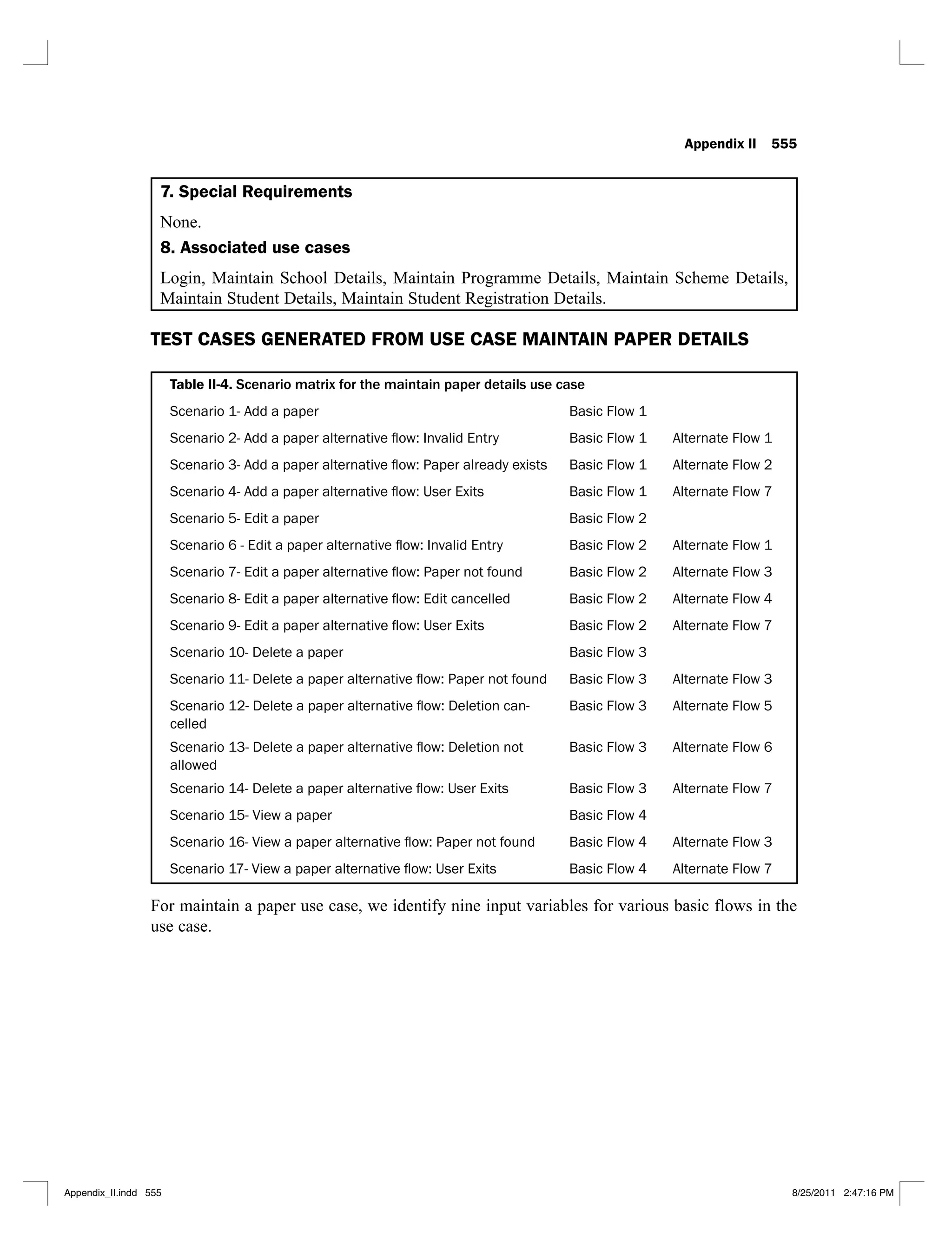
II-4 Scenario matrix for the maintain paper details use case 555
II-5 Test case matrix for the maintain paper details use case 556
xx List of Tables
II-6 Test case matrix with actual data values for the maintain paper details
use case 560
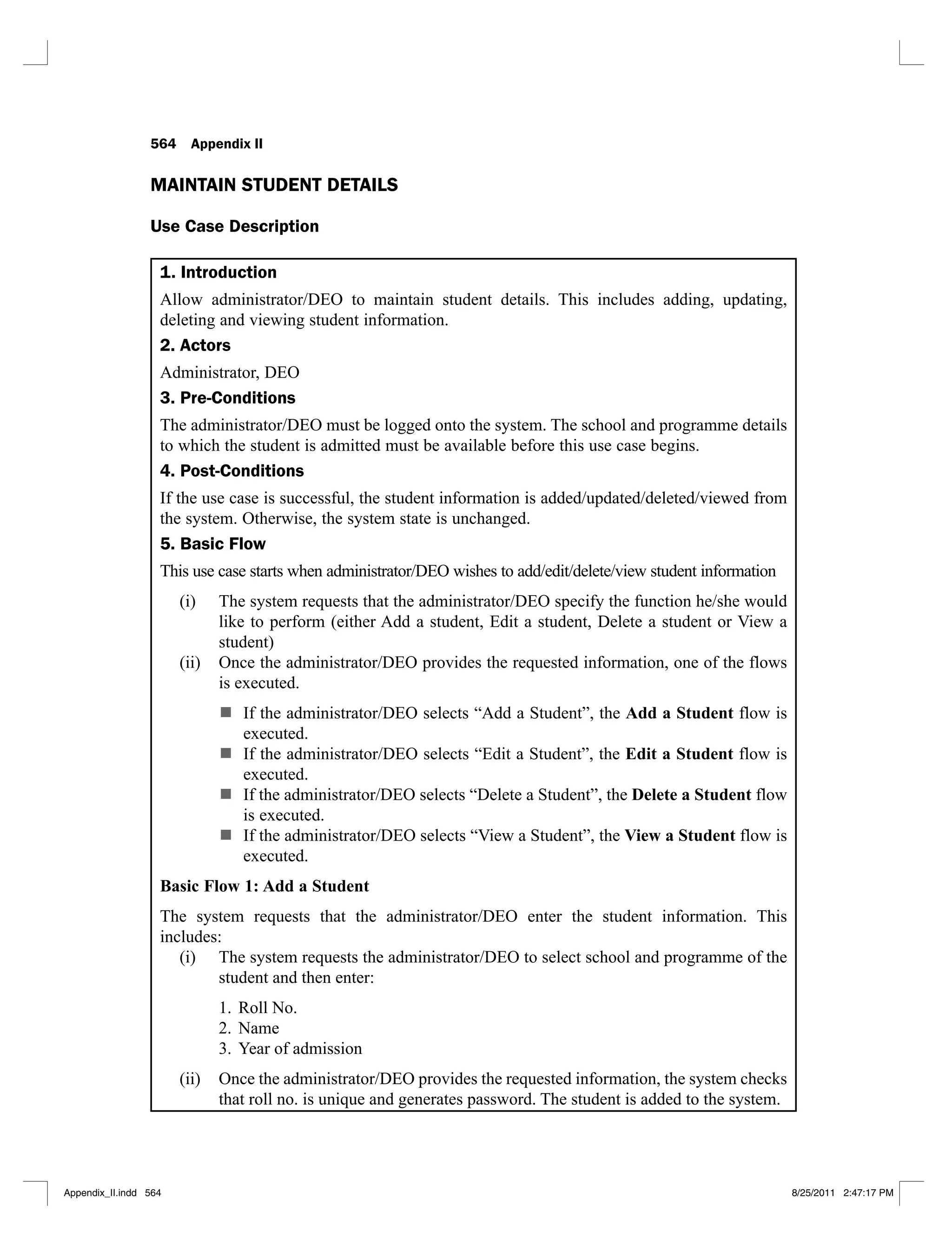
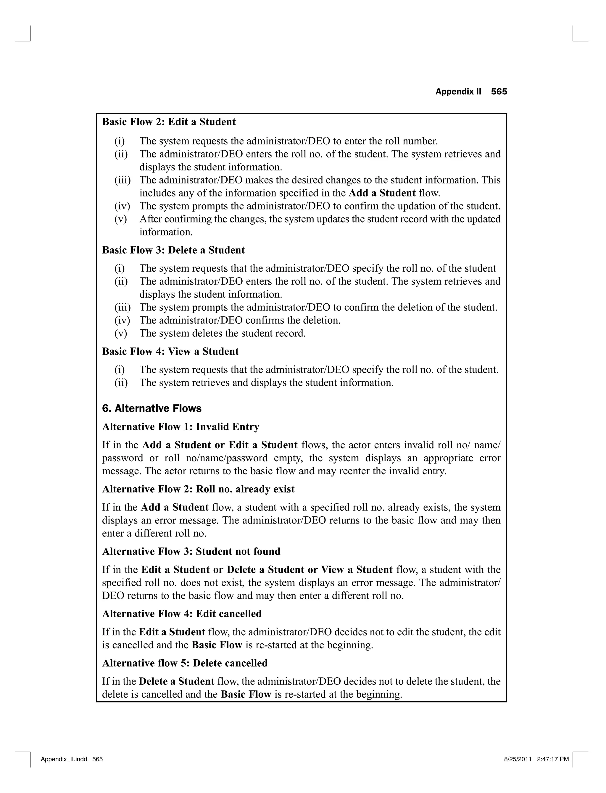
II-7 Scenario matrix for the maintain student details use case 566
II-8 Test case matrix for the maintain student details use case 567
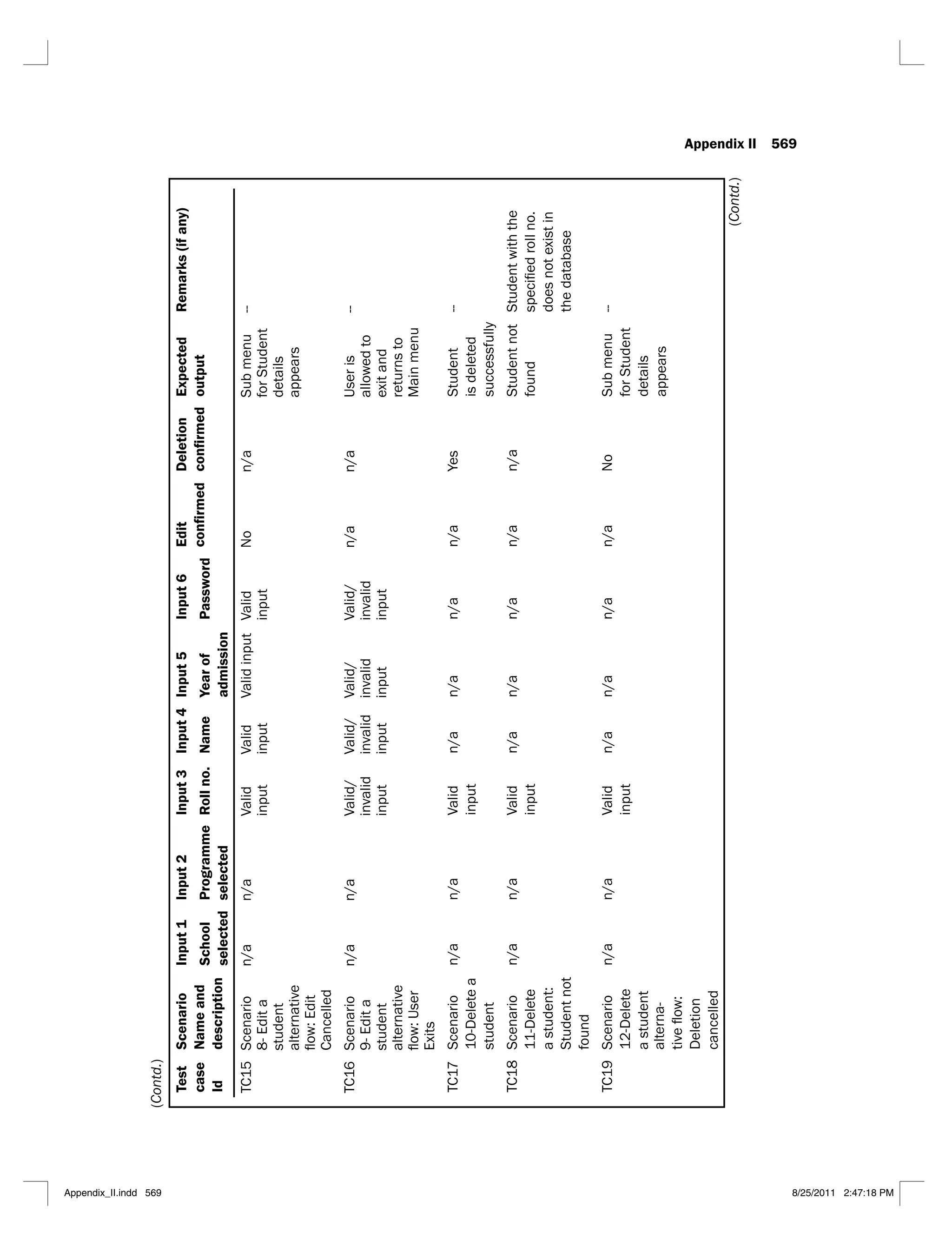
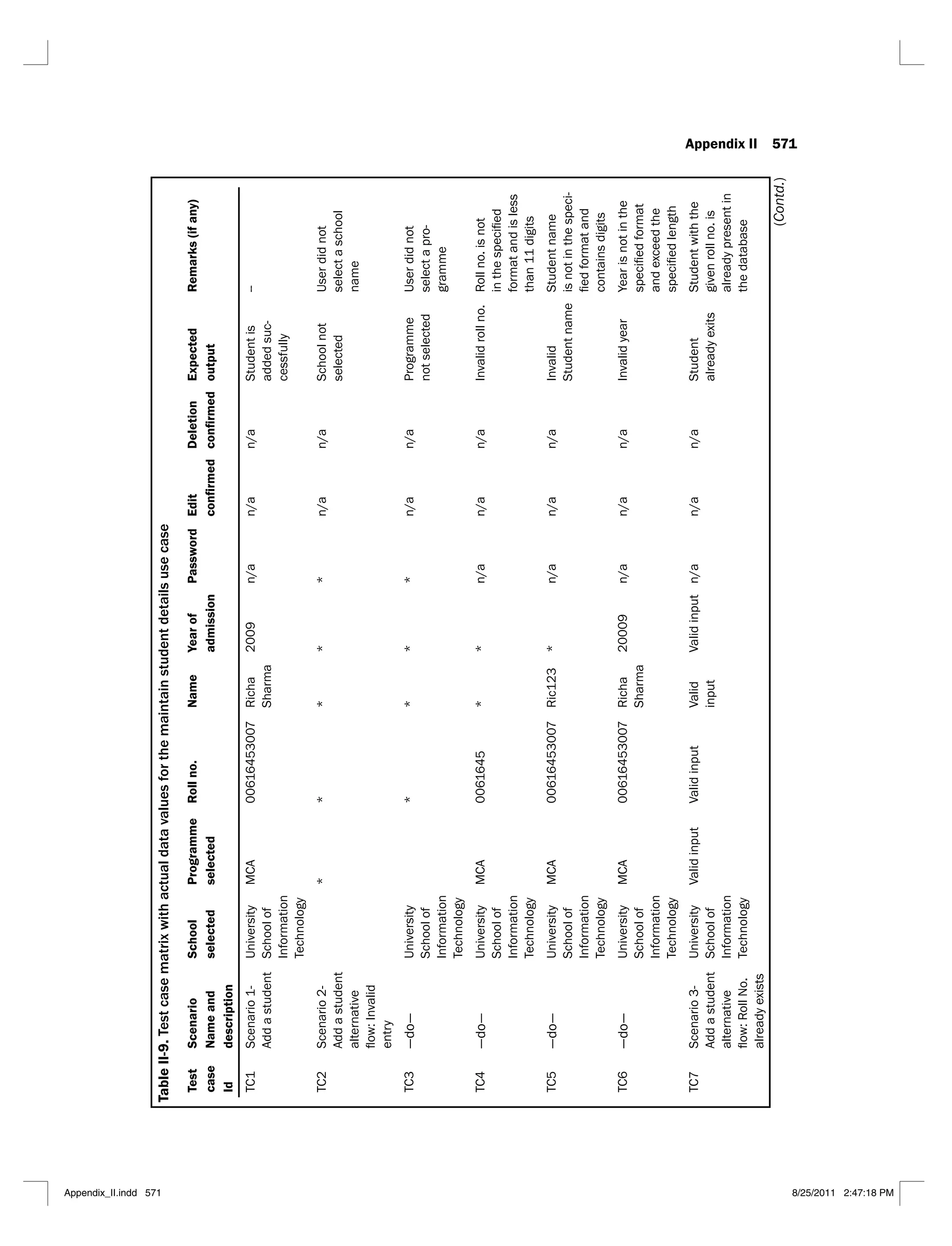
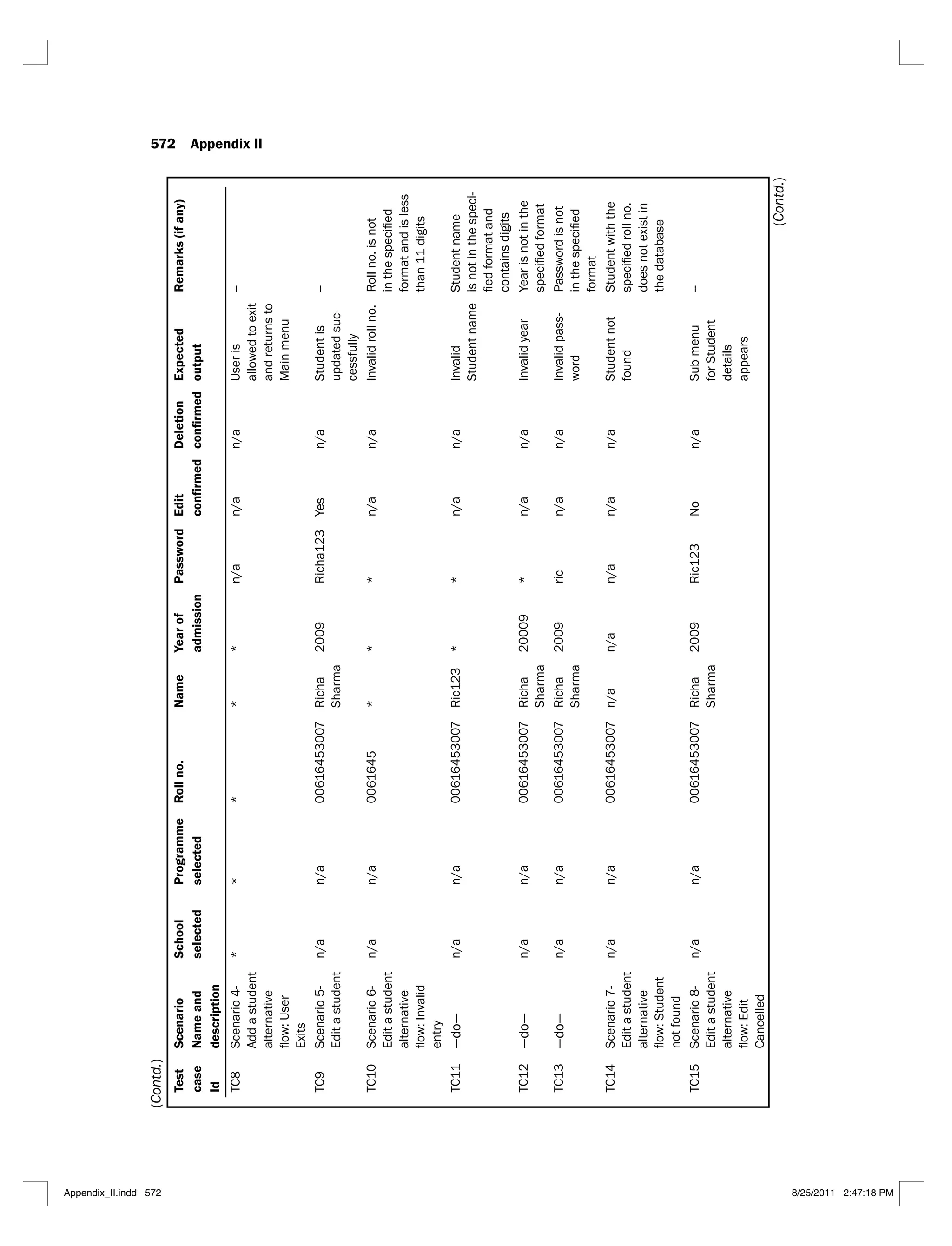
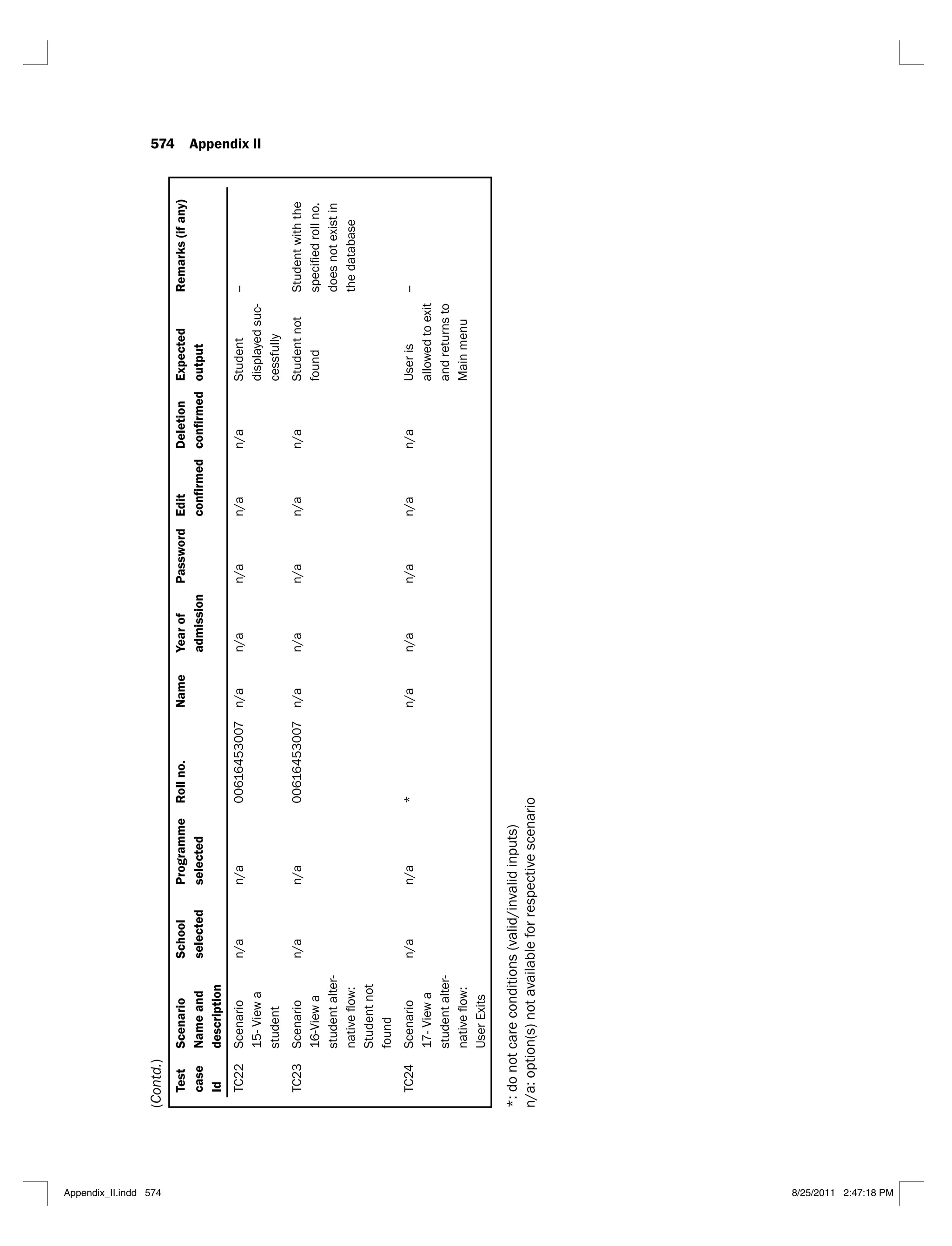
II-9 Test case matrix with actual data values for the maintain student details
use case 571
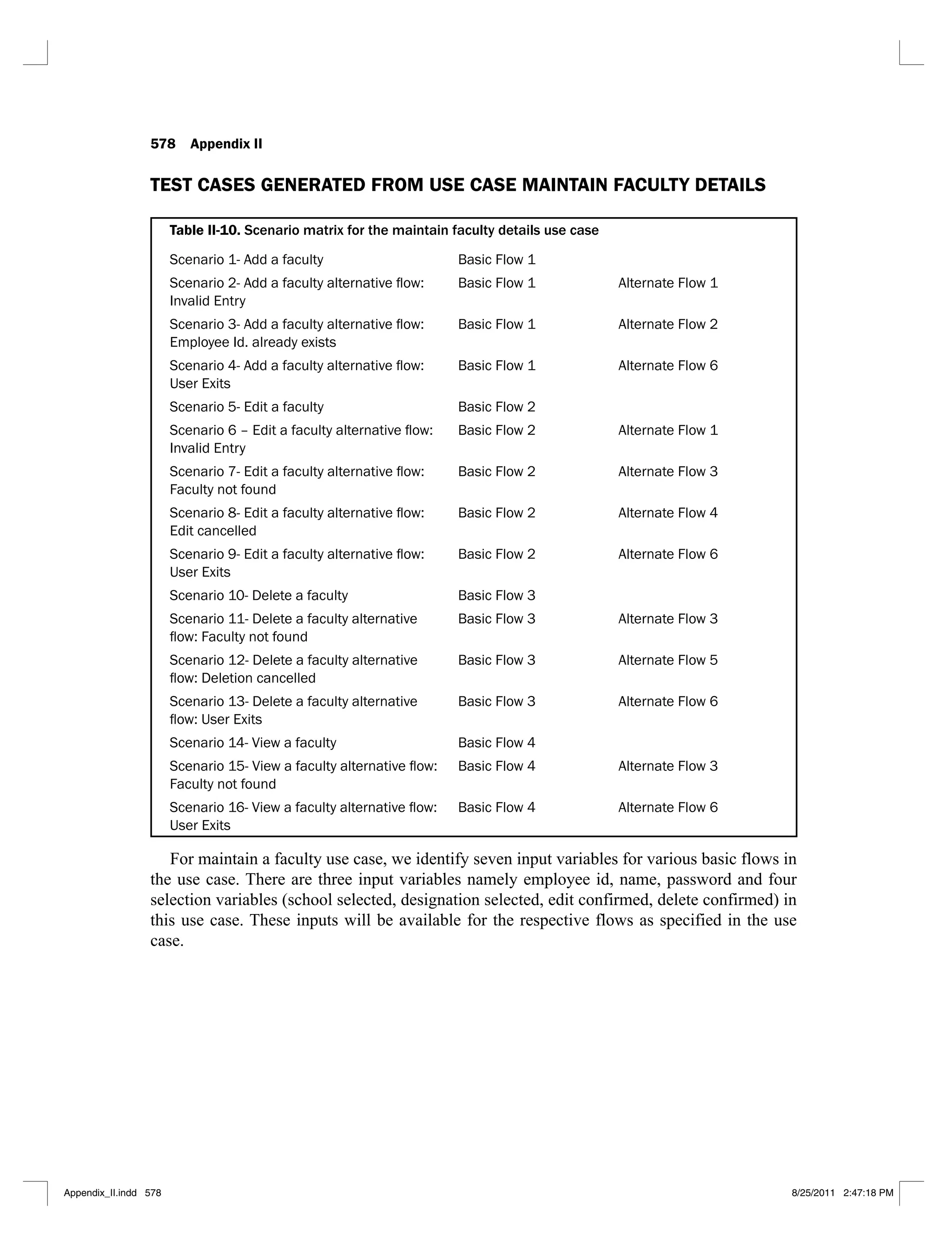
II-10 Scenario matrix for the maintain faculty details use case 578
II-11 Test case matrix for the maintain faculty details use case 579
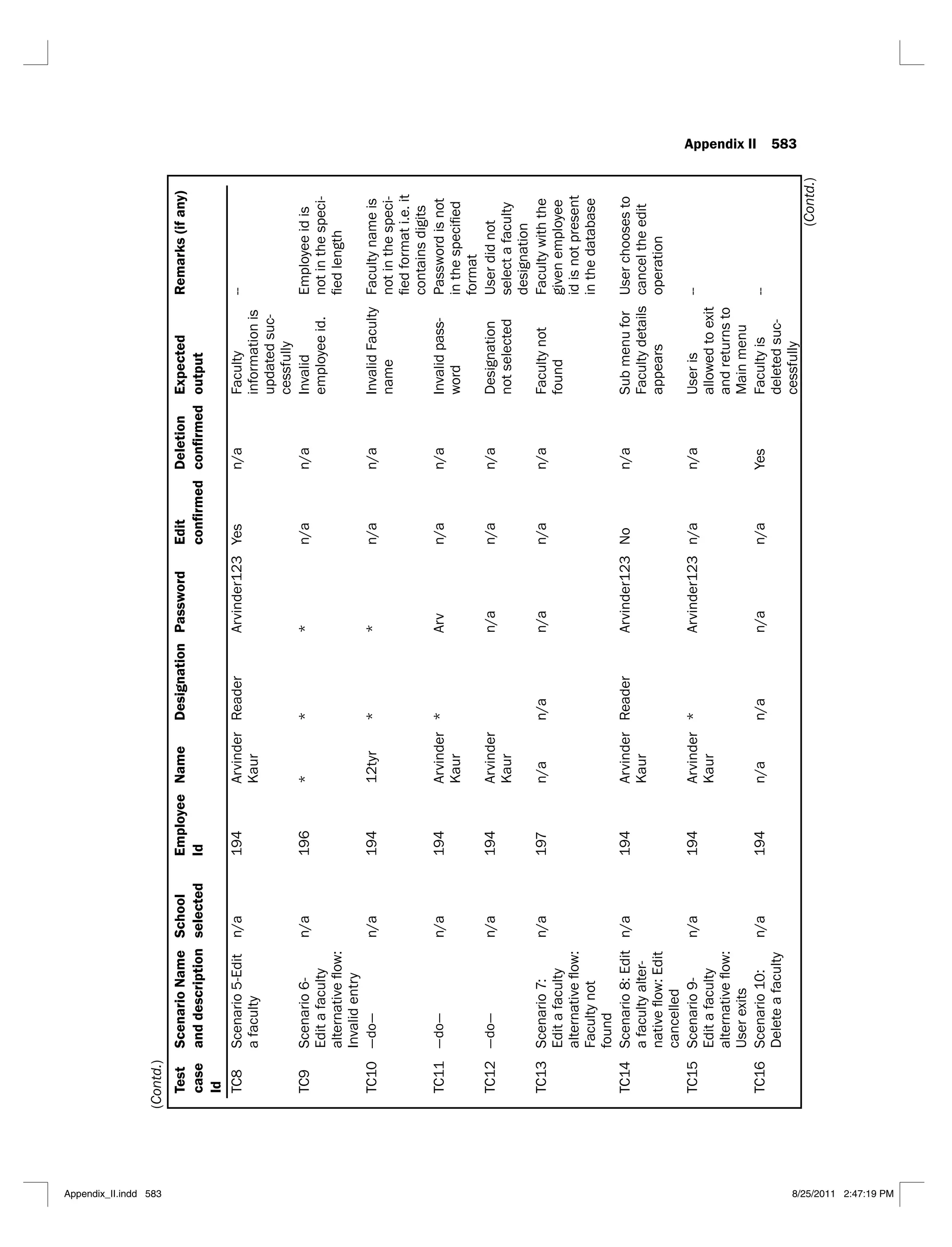
II-12 Test case matrix with actual data values for the maintain faculty details
use case 582
II-13 Scenario matrix for the maintain registration details use case 587
II-14 Test case matrix for the maintain registration details use case 588
II-15 Test case matrix with actual data values for the maintain registration details
use case 591
Preface
There is a worldwide awareness of realizing the importance of software testing. Many
universities now offer a course in software testing for undergraduate and graduate studies in
Computer Science and Engineering, Computer Applications, Information Technology,
Software Engineering and Electronics and Communication Engineering.
The book discusses software testing in the context of testing concepts and methods that can
be implemented in practice. It has been designed as a main textbook for a course in software
testing and as a useful resource for teachers and software practitioners.
The main features of this book are:
It focuses on the importance, significance and limitations of software testing.
It presents functional testing techniques that may help to design test cases without
considering internal structure of the program.
It presents structural testing techniques and introduces some fundamental structural
testing techniques like control flow testing, dataflow testing, slice based testing and
mutation testing.
It promotes verification testing as an integral to modern software testing practices,
equally as important as validation testing. Verification activities such as walkthroughs
and inspections can be carried out at early phases of software development. Use case
testing has also been introduced.
It addresses important issues of selection, minimization and prioritization of test cases
for regression testing. Complementary approaches for achieving adequate number of test
cases during regression testing is also discussed in the book to show how to reduce
maintenance cost.
It presents software testing activities, debugging approaches and testing tools along with
their commercial applications.
It signifies the importance of object oriented testing. It also presents metrics used in
software testing with their practical application in predicting models using commercial
data sets.
It emphasizes on testing web applications covering key areas such as functional testing,
usabilitytesting,userinterfacetesting,securitytesting,performancetesting,configuration
and compatibility testing.
It introduces the concepts of automated test data generation using static and dynamic test
data generation techniques. Genetic algorithm is used for the generation of test data
along with suitable examples.
xxii Preface
The work for this book was primarily collected from the author’s several years of teaching.
Therefore, the text has been thoroughly tested in classroom and revised accordingly in the form
of this textbook. The book contains numerous solved examples and each chapter ends with
multiple choice questions and self-assessment Exercises. The answers to multiple choice
questions have also been provided for verification. An Instructor Manual for teachers is also
available on the website to provide guidance in teaching software testing.
I do realize the importance of feedback of our readers for continuous improvement in the
contents of the book. I shall appreciate the constructive criticism about anything and also about
any omission due to my ignorance. It is expected that the book will be a useful addition in the
literature on software testing. Any suggestion about the book would gratefully be received.
Yogesh Singh
Acknowledgements
This book is the result of hardwork of Dr Ruchika Malhotra, Assistant Professor, Department
of Software Engineering, Delhi Technological University, Delhi. The book would not have
been completed without her kind support.
Thanks to my undergraduate and postgraduate students of the University School of
Information Technology, Guru Gobind Singh Indraprastha University for motivating me to
write this book. Their expectations, discussions and enthusiasm always become my strength
for continuous improvement in academic pursuit. I would also like to thank all researchers,
practitioners, software developers, testers and teachers whose views, ideas and techniques find
a place in this book. I am also grateful to Sandeep Kumar, Stenographer of Examination
Division of the University for typing the draft of the manuscript.
Lastly, I am thankful to Dr Pravin Chandra, Associate Professor, Delhi University, Dr
Jitendra Chabra, Associate Professor, National Institute of Technology, Kurukshetra, Dr
Arvinder Kaur, Associate Professor, Guru Gobind Singh Indraprastha University for their
valuable suggestions. My thanks are also due to Dr Chetna Tiwari, Assistant Professor,
University School of Humanities and Social Sciences, Guru Gobind Singh Indraprastha
University for reading a few chapters of the manuscript.
1
Introduction
What is software testing? Why do we need to test software? Can we live without testing? How
do we handle software bugs reported by the customers? Who should work hard to avoid
frustrations of software failures?
Such questions are endless. But we need to find answers to such burning questions. Software
organizations are regularly getting failure reports of their products and this number is increasing
day by day. All of us would appreciate that it is extremely disappointing for the developers to
receive such failure reports. The developers normally ask: how did these bugs escape unnoticed?
It is a fact that software developers are experiencing failures in testing their coded programs and
such situations are becoming threats to modern automated civilization. We cannot imagine a day
without using cell phones, logging on to the internet, sending e-mails, watching television and
so on. All these activities are dependent on software, and software is not reliable. The world has
seen many software failures and some were even fatal to human life.
1.1 SOME SOFTWARE FAILURES
A major problem of the software industry is its inability to develop error-free software. Had
software developers ever been asked to certify that the software developed is error-free, no
software would have ever been released. Hence ‘software crises’ has become a fixture of
everyday life with many well-publicized failures that have had not only major economic
impact but also have become the cause of loss of life. Some of the failures are discussed in
subsequent sections.
1.1.1 The Explosion of the Ariane 5 Rocket
The Ariane 5 rocket was designed by European Space Agency and it was launched on June 4,
1996. It was an unmanned rocket and unfortunately exploded only after 40 seconds of its take
2 Software Testing
off from Kourou, French Guiana. The design and development took ten long years with a cost
of $7 billion. An enquiry board was constituted to find the reasons of the explosion. The board
identified the cause and mentioned in its report that [LION96]: “The failure of the Ariane 5
was caused by the complete loss of guidance and altitude information, 37 seconds after start of
the main engine ignition sequence (30 seconds after lift-off). This loss of information was due
to specification and design errors in the software of the inertial reference system. The extensive
reviews and tests carried out during the Ariane 5 development programme did not include
adequate analysis and testing of the inertial reference system or of the complete flight control
system, which could have detected the potential failure”. A software fault in the inertial
reference system was identified as a reason for the explosion by the enquiry committee. The
inertial reference system of the rocket had tried to convert 64 bit floating point number of
horizontal velocity to a 16 bit signed integer. However, the number was greater than 32,767
(beyond the permissible limit of 16 bit machine) and the conversion process failed.
Unfortunately, the navigation system of Ariane 4 was used in Ariane 5 without proper
testing and analysis. The Ariane 5 was a high speed rocket with higher value of an internal
alignment function, known as horizontal bias. This value is for the calculation of horizontal
velocity. On the day of the explosion, this value was more than expectations due to different
trajectory of this rocket as compared to the Ariane 4. Therefore, the main technical reason was
the conversion problem at the time of converting the horizontal bias variable, and this resulted
into the shutdown of the computer of the inertial reference system. When the computer shut
down, it passed control to an identical, redundant unit, which was there to provide backup in
case of such a failure. But the second unit had failed in the identical manner before a few
milliseconds. Why wouldn’t it be? It was running the same software.
The designers never thought that the particular velocity value would ever be large enough
to cause trouble. After all, it never had been before. Unfortunately Ariane 5 was a faster rocket
than Ariane 4. Moreover, the calculation containing the error, which shut down the computer
system, actually served no purpose, once the rocket was in the air. Its only function was to
align the system before launch. So it should have been turned off. But designers chose long
ago, in an earlier version of the Ariane 4, to leave this function running for the first forty
seconds of flight – a ‘special feature’ meant to make the restart of the system easy in the event
of a brief hold in the countdown. Such design decisions and poor testing resulted in the
explosion of Ariane 5.
1.1.2 The Y2K Problem
The Y2K problem was the most critical problem of the last century. The whole world was
expecting something drastic on January 1, 2000. Significant sums of money were spent by
software companies to get rid of this problem. What was the problem? It was simply the case
of using two digits for the year instead of four digits. For instance, 1965 was considered as 65.
The developers could not imagine the problem of year 2000. What would happen on January
1, 2000? The last two digits i.e. 00 may belong to any century like 1800, 1900, 2000, 2100,
etc. The simple ignorance or a faulty design decision to use only the last two digits for the year
resulted into the serious Y2K problem. Most of the software was re-tested and modified or
discarded, depending on the situation.
Introduction 3
1.1.3 The USA Star-Wars Program
‘Patriot missile’ was the result of the USA ‘Star Wars’ program. This missile was used for the
first time in the Gulf war against the Scud missile of Iraq. Surprisingly, ‘Patriot missiles’ failed
many times to hit the targeted Scud missile. One of the failures killed 28 American soldiers in
Dhahran, Saudi Arabia. An investigation team was constituted to identify the cause of failure.
The team re-looked at every dimension of the product and found the reason for the failure. The
cause of the failure was a software fault. There was a slight timing error in the system’s clock
after 14 hours of its operation. Hence, the tracking system was not accurate after 14 hours of
operations and at the time of the Dhahran attack, the system had already operated for more than
100 hours.
1.1.4 Failure of London Ambulance System
The software controlling the ambulance dispatch system of London collapsed on October
26-27, 1992 and also on November 4, 1992 due to software failures. The system was introduced
on October 26, 1992. The London Ambulance Service was a challenging task that used to
cover an area of 600 square miles and handled 1500 emergency calls per day. Due to such a
failure, there was a partial or no ambulance cover for many hours. The position of the vehicles
was incorrectly recorded and multiple vehicles were sent to the same location. Everywhere
people were searching for an ambulance and nobody knew the reason for non-arrival of
ambulances at the desired sites. The repair cost was estimated to be £9m, but it is believed that
twenty lives could have been saved if this failure had not occurred. The enquiry committee
clearly pointed out the administrative negligence and over-reliance on ‘cosy assurances’ of the
software company. The administration was allowed to use this system without proper
alternative systems in case of any failure. The committee also termed the possible cause of
failure as [ANDE98, FINK93]: “When the system went live, it could not cope with the volume
of calls and broke under the strain. The transition to a back-up computer system had not been
properly rehearsed and also failed.”
1.1.5 USS Yorktown Incident
The USS Yorktown - a guided missile cruiser was in the water for several hours due to the
software failure in 1998. A user wrongly gave a zero value as an input which caused a division
by zero error. This fault further failed the propulsion system of the ship and it did not move in
the water for many hours. The reason behind this failure was that the program did not check
for any valid input.
1.1.6 Accounting Software Failures
Financial software is an essential part of any company’s IT infrastructure. However, many
companies have suffered failures in the accounting system due to errors in the financial software.
The failures range from producing the wrong information to the complete system failure. There
4 Software Testing
is widespread dissatisfaction over the quality of financial software. If a system gives information
in the incorrect format, it may have an adverse impact on customer satisfaction.
1.1.7 Experience of Windows XP
Charles C. Mann shared his views about Windows XP through his article in technology review
[MANN02] as: “Microsoft released Windows XP on October 25, 2001. That same day, what
may be a record, the company posted 18 megabyte of patches on its website for bug fixes,
compatibility updates, and enhancements. Two patches fixed important security holes. Or
rather, one of them did; the other patch did not work. Microsoft advised (still advises) users to
back up critical files before installing patches.” This situation is quite embarrassing and clearly
explains the sad situation of the software companies. The developers were either too careless
or in a great hurry to fix such obvious faults.
We may endlessly continue discussing the history of software failures. Is there any light at
the end of the tunnel? Or will the same scenario continue for many years to come? When
automobile engineers give their views about cars, they do not say that the quality of today’s
cars is not better than the cars produced in the last decade. Similarly aeronautical engineers do
not say that Boeing orAirbus makes poor quality planes as compared to the planes manufactured
in the previous decade. Civil engineers also do not show their anxieties over the quality of
today’s structures over the structures of the last decade. Everyone feels that things are
improving day by day. But software, alas, seems different. Most of the software developers are
confused about the quality of their software products. If they are asked about the quality of
software being produced by companies, they generally say, “It is getting worse day by day.” It
is as if we say that Boeing’s planes produced in 2009 are less reliable than those produced in
1980. The blame for software bugs belongs to nearly everyone. It belongs to the software
companies that rush products to market without adequately testing them. It belongs to the
software developers who do not understand the importance of detecting and removing faults
before customers experience them as failures. It belongs to a legal system that has given the
software developers a free pass on error-related damages. The blame also belongs to universities
that stress more on software development than testing.
1.2 TESTING PROCESS
Testing is an important aspect of the software development life cycle. It is basically the
process of testing the newly developed software, prior to its actual use. The program is
executed with desired input(s) and the output(s) is/are observed accordingly. The observed
output(s) is/are compared with expected output(s). If both are same, then the program is said
to be correct as per specifications, otherwise there is something wrong somewhere in the
program. Testing is a very expensive process and consumes one-third to one-half of the cost
of a typical development project. It is largely a systematic process but partly intuitive too.
Hence, good testing process entails much more than just executing a program a few times to
see its correctness.
Introduction 5
1.2.1 What is Software Testing?
Good testing entails more than just executing a program with desired input(s). Let’s consider
a program termed as ‘Minimum’ (see Figure 1.1) that reads a set of integers and prints the
smallest integer. We may execute this program using Turbo C complier with a number of inputs
and compare the expected output with the observed output as given in Table 1.1.
LINE NUMBER /*SOURCE CODE*/
#include<stdio.h>
#include<limits.h>
#include<conio.h>
1. void Minimum();
2. void main()
3. {
4. Minimum();
5. }
6. void Minimum()
7. {
8. int array[100];
9. int Number;
10. int i;
11. int tmpData;
12. int Minimum=INT_MAX;
13. clrscr();
14. "printf("Enter the size of the array:");
15. scanf("%d",&Number);
16. for(i=0;i<Number;i++) {
17. printf("Enter A[%d]=",i+1);
18. scanf("%d",&tmpData);
19. tmpData=(tmpData<0)?-tmpData:tmpData;
20. array[i]=tmpData;
21. }
22. i=1;
23. while(i<Number-1) {
24. if(Minimum>array[i])
25. {
26. Minimum=array[i];
27. }
28. i++;
29. }
30. printf("Minimum = %dn", Minimum);
31. getch();
32. }
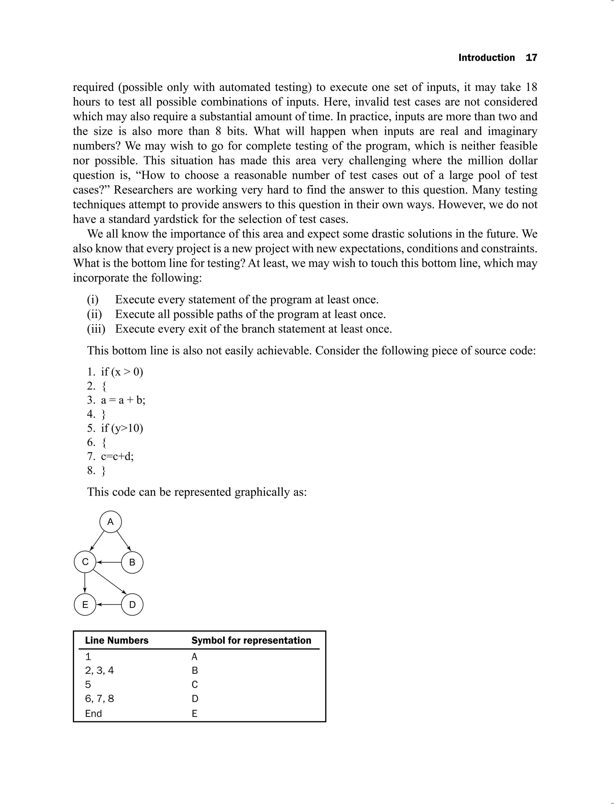
Figure 1.1. Program ‘Minimum’ to find the smallest integer out of a set of integers
6 Software Testing
Table 1.1. Inputs and outputs of the program ‘Minimum’
Test Case Inputs Expected
Output
Observed
Output
Match?
Size Set of Integers
1. 5 6, 9, 2, 16, 19 2 2 Yes
2. 7 96, 11, 32, 9, 39, 99, 91 9 9 Yes
3. 7 31, 36, 42, 16, 65, 76, 81 16 16 Yes
4. 6 28, 21, 36, 31, 30, 38 21 21 Yes
5. 6 106, 109, 88, 111, 114, 116 88 88 Yes
6. 6 61, 69, 99, 31, 21, 69 21 21 Yes
7. 4 6, 2, 9, 5 2 2 Yes
8. 4 99, 21, 7, 49 7 7 Yes
There are 8 sets of inputs in Table 1.1. We may feel that these 8 test cases are sufficient for
such a trivial program. In all these test cases, the observed output is the same as the expected
output. We may also design similar test cases to show that the observed output is matched with
the expected output. There are many definitions of testing. A few of them are given below:
(i) Testing is the process of demonstrating that errors are not present.
(ii) The purpose of testing is to show that a program performs its intended functions
correctly.
(iii) Testing is the process of establishing confidence that a program does what it is supposed
to do.
The philosophy of all three definitions is to demonstrate that the given program behaves as
per specifications. We may write 100 sets of inputs for the program ‘Minimum’ and show that
this program behaves as per specifications. However, all three definitions are not correct. They
describe almost the opposite of what testing should be viewed as. Forgetting the definitions for
the moment, whenever we want to test a program, we want to establish confidence about the
correctness of the program. Hence, our objective should not be to show that the program works
as per specifications. But, we should do testing with the assumption that there are faults and
our aim should be to remove these faults at the earliest. Thus, a more appropriate definition is
[MYER04]: “Testing is the process of executing a program with the intent of finding
faults.” Human beings are normally goal oriented. Thus, establishment of a proper objective
is essential for the success of any project. If our objective is to show that a program has no
errors, then we shall sub-consciously work towards this objective. We shall intend to choose
those inputs that have a low probability of making a program fail as we have seen in Table 1.1,
where all inputs are purposely selected to show that the program is absolutely correct. On the
contrary, if our objective is to show that a program has errors, we may select those test cases
which have a higher probability of finding errors. We shall focus on weak and critical portions
of the program to find more errors. This type of testing will be more useful and meaningful.
We again consider the program ‘Minimum’ (given in Figure 1.1) and concentrate on some
typical and critical situations as discussed below:
A very short list (of inputs) with the size of 1, 2, or 3 elements.
(i)
An empty list i.e. of size 0.
(ii)
Introduction 7
A list where the minimum element is the first or last element.
(iii)
A list where the minimum element is negative.
(iv)
A list where all elements are negative.
(v)
A list where some elements are real numbers.
(vi)
A list where some elements are alphabetic characters.
(vii)
A list with duplicate elements.
(viii)
A list where one element has a value greater than the maximum permissible limit of an
(ix)
integer.
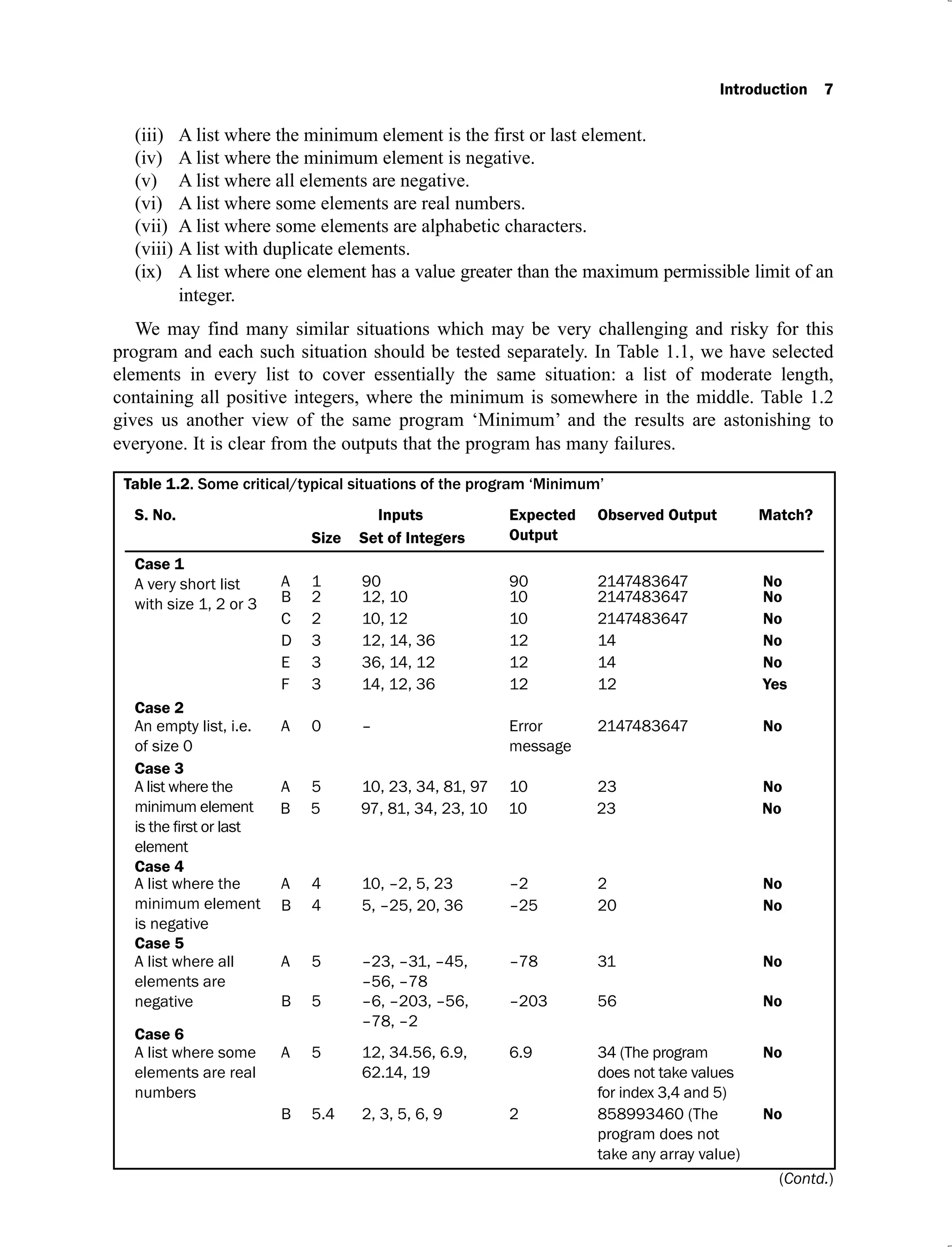
We may find many similar situations which may be very challenging and risky for this
program and each such situation should be tested separately. In Table 1.1, we have selected
elements in every list to cover essentially the same situation: a list of moderate length,
containing all positive integers, where the minimum is somewhere in the middle. Table 1.2
gives us another view of the same program ‘Minimum’ and the results are astonishing to
everyone. It is clear from the outputs that the program has many failures.
Table 1.2. Some critical/typical situations of the program ‘Minimum’
S. No. Inputs Expected
Output
Observed Output Match?
Size Set of Integers
Case 1
A very short list
with size 1, 2 or 3
A 1 90 90 2147483647 No
B 2 12, 10 10 2147483647 No
C 2 10, 12 10 2147483647 No
D 3 12, 14, 36 12 14 No
E 3 36, 14, 12 12 14 No
F 3 14, 12, 36 12 12 Yes
Case 2
An empty list, i.e.
of size 0
A 0 – Error
message
2147483647 No
Case 3
A list where the
minimum element
element
A 5 10, 23, 34, 81, 97 10 23 No
B 5 97, 81, 34, 23, 10 10 23 No
Case 4
A list where the
minimum element
is negative
A 4 10, –2, 5, 23 –2 2 No
B 4 5, –25, 20, 36 –25 20 No
Case 5
A list where all
elements are
negative
A 5 –23, –31, –45,
–56, –78
–78 31 No
B 5 –6, –203, –56,
–78, –2
–203 56 No
Case 6
A list where some
elements are real
numbers
A 5 12, 34.56, 6.9,
62.14, 19
6.9 34 (The program
does not take values
for index 3,4 and 5)
No
B 5.4 2, 3, 5, 6, 9 2 858993460 (The
program does not
take any array value)
No
(Contd.)
8 Software Testing
S. No. Inputs Expected
Output
Observed Output Match?
Size Set of Integers
Case 7
A list where some
elements are
characters
A 5 23, 2I, 26, 6, 9 6 2 (The program does
not take any other
index value for 3, 4
and 5)
No
B 1I 2, 3, 4, 9, 6, 5,
11, 12, 14, 21, 22
2 2147483647
(Program does not
take any other index
value)
No
Case 8
A list with dupli-
cate elements
A 5 3, 4, 6, 9, 6 3 4 No
B 5 13, 6, 6, 9, 15 6 6 Yes
Case 9
A list where one
element has a
value greater than
the maximum
permissible limit
of an integer
A 5 530,
4294967297, 23,
46, 59
23 1 No
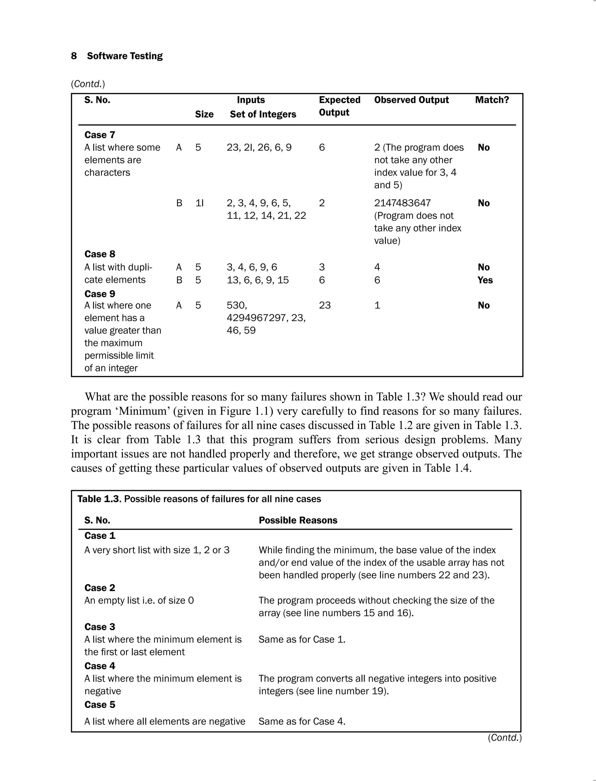
What are the possible reasons for so many failures shown in Table 1.3? We should read our
program ‘Minimum’ (given in Figure 1.1) very carefully to find reasons for so many failures.
The possible reasons of failures for all nine cases discussed in Table 1.2 are given in Table 1.3.
It is clear from Table 1.3 that this program suffers from serious design problems. Many
important issues are not handled properly and therefore, we get strange observed outputs. The
causes of getting these particular values of observed outputs are given in Table 1.4.
Table 1.3. Possible reasons of failures for all nine cases
S. No. Possible Reasons
Case 1
A very short list with size 1, 2 or 3
and/or end value of the index of the usable array has not
been handled properly (see line numbers 22 and 23).
Case 2
An empty list i.e. of size 0 The program proceeds without checking the size of the
array (see line numbers 15 and 16).
Case 3
A list where the minimum element is Same as for Case 1.
Case 4
A list where the minimum element is
negative
The program converts all negative integers into positive
integers (see line number 19).
Case 5
A list where all elements are negative Same as for Case 4.
(Contd.)
(Contd.)
Introduction 9
S. No. Possible Reasons
Case 6
A list where some elements are real
numbers
The program uses scanf() function to read the values. The
scanf() has unpredictable behaviour for inputs not accord-
Case 7
A list where some elements are
alphabetic characters
Same as for Case 6.
Case 8
A list with duplicate elements (a) Same as for Case 1.
(b) We are getting the correct result because the minimum
value is in the middle of the list and all values are positive.
Case 9
A list with one value greater than
the maximum permissible limit of an
integer
This is a hardware dependent problem. This is the case
integer. In this example, 32 bits integers are used.
Table 1.4. Reasons for observed output
Cases Observed Output Remarks
1 (a)
1 (b)
1 (c)
2147483647
2147483647
2147483647
the maximum value of a 32 bit integer to which a variable minimum
is initialized.
1 (d)
1 (e)
14
14 middle value is 14.
1 (f) 12
Fortunately, the middle value is the minimum value and thus the
result is correct.
2 (a) 2147483647 The maximum value of a 32 bit integer to which a variable minimum
is initialized.
3 (a)
3 (b)
23
23 value 23 is the minimum value in the remaining list.
4 (a)
4 (b)
2
20 converted negative integer(s) to positive integer(s).
5 (a)
5 (b)
31
56
Same as Case 4.
6 (a) 34 After getting ‘.’ of 34.56, the program was terminated and 34 was
displayed. However, the program has also ignored 12, being the
6 (b) 858993460 Garbage value.
7 (a) 2 After getting ‘I’ in the second index value ‘2I’, the program
terminated abruptly and displayed 2.
7 (b) 2147483647 The input has a non digit value. The program displays the value to
which variable ‘minimum’ is initialized.
8 (a) 4
minimum in the remaining list.
8 (b) 6
values are ignored.
9 (a) 1
signed integer data type used in the program.
(Contd.)
10 Software Testing
Modifications in the program ‘Minimum’
Table 1.4 has given many reasons for undesired outputs. These reasons help us to identify the
causes of such failures. Some important reasons are given below:
The program has ignored the first and last values of the list
(i)
The program is not handling the first and last values of the list properly. If we see the
line numbers 22 and 23 of the program, we will identify the causes. There are two
faults. Line number 22 “i = 1;” should be changed to “i = 0;” in order to handle the first
value of the list. Line number 23 “while (i<Number -1)” should be changed to “while
(i<=Number-1)” in order to handle the last value of the list.
The program proceeds without checking the size of the array
(ii)
If we see line numbers 14 and 15 of the program, we will come to know that the program
is not checking the size of the array / list before searching for the minimum value. A list
cannot be of zero or negative size. If the user enters a negative or zero value of size or value
greater than the size of the array, an appropriate message should be displayed. Hence after
line number 15, the value of the size should be checked as under:
if (Number < = 0||Number>100)
{
printf ("Invalid size specified");
}
If the size is greater than zero and lesser than 101, then the program should proceed
further, otherwise it should be terminated.
Program has converted negative values to positive values
(iii)
Line number 19 is converting all negative values to positive values. That is why the
program is not able to handle negative values. We should delete this line to remove
this fault.
The modified program, based on the above three points is given in Figure 1.2. The nine
cases of Table 1.2 are executed on this modified program and the results are given in
Table 1.5.
LINE NUMBER /*SOURCE CODE*/
#include<stdio.h>
#include<limits.h>
#include<conio.h>
1. void Minimum();
2. void main()
3. {
4. Minimum();
5. }
6. void Minimum()
7. {
8. int array[100];
9. int Number;
(Contd.)
Introduction 11
10. int i;
11. int tmpData;
12. int Minimum=INT_MAX;
13. clrscr();
14. printf("Enter the size of the array:");
15. scanf("%d",&Number);
16. if(Number<=0||Number>100) {
17. printf("Invalid size specified");
18. }
19. else {
20. for(i=0;i<Number;i++) {
21. printf("Enter A[%d]=",i+1);
22. scanf("%d",&tmpData);
23. /*tmpData=(tmpData<0)?-tmpData:tmpData;*/
24. array[i]=tmpData;
25. }
26. i=0;
27. while(i<=Number-1) {
28. if(Minimum>array[i])
29. {
30. Minimum=array[i];
31. }
32. i++;
33. }
34. printf("Minimum = %dn", Minimum);
35. }
36. getch();
37. }
Figure 1.2. Modified program ‘Minimum’ to find the smallest integer out of a set of integers
Table 1.5 gives us some encouraging results. Out of 9 cases, only 3 cases are not matched.
Six cases have been handled successfully by the modified program given in Figure 1.2. The
cases 6 and 7 are failed due to the scanf() function parsing problem. There are many ways to
handle this problem. We may design a program without using scanf() function at all.
However, scanf() is a very common function and all of us use it frequently. Whenever any
value is given using scanf() which is not as per specified format, scanf() behaves very
notoriously and gives strange results. It is advisable to display a warning message for the user
before using the scanf() function. The warning message may compel the user to enter values
in the specified format only. If the user does not do so, he/she may have to suffer the
consequences accordingly. The case 9 problem is due to the fixed maximal size of the
integers in the machine and the language used. This also has to be handled through a warning
message to the user. The further modified program based on these observations is given in
the Figure 1.3.
(Contd.)
12 Software Testing
Table 1.5
Sr. No.
Inputs Expected
Output
Observed
Output
Match?
Size Set of Integers
Case 1
A very short list with
size 1, 2 or 3
A 1 90 90 90 Yes
B 2 12, 10 10 10 Yes
C 2 10, 12 10 10 Yes
D 3 12, 14, 36 12 12 Yes
E 3 36, 14, 12 12 12 Yes
F 3 14, 12, 36 12 12 Yes
Case 2
An empty list, i.e. of
size 0
A 0 – Error
message
Error
message
Yes
Case 3
A list where the mini-
mum element is the
A 5 10, 23, 34, 81, 97 10 10 Yes
B 5 97, 81, 34, 23, 10 10 10 Yes
Case 4
A list where the
minimum element is
negative
A 4 10, –2, 5, 23 –2 –2 Yes
B 4 5, –25, 20, 36 –25 –25 Yes
Case 5
A list where all
elements are
negative
A 5 –23, –31, –45,
–56, –78
–78 –78 Yes
B 5 –6, –203, –56,
–78, –2
–203 –203 Yes
Case 6
A list where some
elements are real
numbers
A 5 12, 34.56, 6.9,
62.14, 19
6.9 34 No
B 5.4 2, 3, 5, 6, 9 2 858993460 No
Case 7
A list where some ele-
ments are alphabetic
characters
A 5 23, 2I, 26, 6, 9 6 2 No
B 1I 2, 3, 4, 9, 6, 5, 11,
12, 14, 21, 22
2 858993460 No
Case 8
A list with duplicate
elements
A 5 3,4,6,9, 6 3 3 Yes
B 5 13, 6, 6, 9, 15 6 6 Yes
Case 9
A list where one
element has a value
greater than the maxi-
mum permissible limit
of an integer
A 5 530, 42949672
97, 23, 46, 59
23 1 No
Introduction 13
LINE NUMBER /*SOURCE CODE*/
#include<stdio.h>
#include<limits.h>
#include<conio.h>
1. void Minimum();
2. void main()
3. {
4. Minimum();
5. }
6. void Minimum()
7. {
8. int array[100];
9. int Number;
10. int i;
11. int tmpData;
12. int Minimum=INT_MAX;
13. clrscr();
14. printf("Enter the size of the array:");
15. scanf("%d",&Number);
16. if(Number<=0||Number>100) {
17. printf("Invalid size specified");
18. }
19. else {
20. printf("Warning: The data entered must be a valid integer and
must be between %d to %d, INT_MIN, INT_MAXn");
21. for(i=0;i<Number;i++) {
22. printf("Enter A[%d]=",i+1);
23. scanf("%d",&tmpData);
24. /*tmpData=(tmpData<0)?-tmpData:tmpData;*/
25. array[i]=tmpData;
26. }
27. i=0;
28. while(i<=Number-1) {
29. if(Minimum>array[i])
30. {
31. Minimum=array[i];
32. }
33. i++;
34. }
35. printf("Minimum = %dn", Minimum);
36. }
37. getch();
38. }
Figure 1.3. Final program ‘Minimum’ to find the smallest integer out of a set of integers
14 Software Testing
Our goal is to find critical situations of any program. Test cases shall be designed for every
critical situation in order to make the program fail in such situations. If it is not possible to remove
a fault then proper warning messages shall be given at proper places in the program. The aim of
the best testing person should be to fix most of the faults. This is possible only if our intention is
to show that the program does not work as per specifications. Hence, as given earlier, the most
appropriate definition is “Testing is the process of executing a program with the intent of
finding faults.” Testing never shows the absence of faults, but it shows that the faults are present
in the program.
1.2.2 Why Should We Test?
Software testing is a very expensive and critical activity; but releasing the software without
testing is definitely more expensive and dangerous. No one would like to do it. It is like
running a car without brakes. Hence testing is essential; but how much testing is required? Do
we have methods to measure it? Do we have techniques to quantify it? The answer is not easy.
All projects are different in nature and functionalities and a single yardstick may not be helpful
in all situations. It is a unique area with altogether different problems.
The programs are growing in size and complexity. The most common approach is ‘code and
fix’ which is against the fundamental principles of software engineering. Watts S. Humphrey,
of Carnegie Mellon University [HUMP02] conducted a multiyear study of 13000 programs
and concluded that “On average professional coders make 100 to 150 errors in every thousand
lines of code they write.” The C. Mann [MANN02] used Humphrey’s figures on the business
operating system Windows NT 4 and gave some interesting observations: “Windows NT 4
code size is of 16 million lines. Thus, this would have been written with about two million
mistakes. Most would have been too small to have any effect, but some thousands would have
caused serious problems. Naturally, Microsoft exhaustively tested Windows NT 4 before
release, but in almost any phase of tests, they would have found less than half the defects. If
Microsoft had gone through four rounds of testing, an expensive and time consuming
procedure, the company would have found at least 15 out of 16 bugs. This means five defects
per thousand lines of code are still remaining. This is very low. But the software would still
have (as per study) as many as 80,000 defects.”
The basic issue of this discussion is that we cannot release a software system without
adequate testing. The study results may not be universally applicable but, at least, they give us
some idea about the depth and seriousness of the problem. When to release the software is a
very important decision. Economics generally plays an important role. We shall try to find
more errors in the early phases of software development. The cost of removal of such errors
will be very reasonable as compared to those errors which we may find in the later phases of
software development. The cost to fix errors increases drastically from the specification phase
to the test phase and finally to the maintenance phase as shown in Figure 1.4.
If an error is found and fixed in the specification and analysis phase, it hardly costs anything.
We may term this as ‘1 unit of cost’ for fixing an error during specifications and analysis
phase. The same error, if propagated to design, may cost 10 units and if, further propagated to
coding, may cost 100 units. If it is detected and fixed during the testing phase, it may lead to
1000 units of cost. If it could not be detected even during testing and is found by the customer
after release, the cost becomes very high. We may not be able to predict the cost of failure for
Introduction 15
a life critical system’s software. The world has seen many failures and these failures have been
costly to the software companies.
The fact is that we are releasing software that is full of errors, even after doing sufficient
testing. No software would ever be released by its developers if they are asked to certify that
the software is free of errors. Testing, therefore, continues to the point where it is considered
that the cost of testing processes significantly outweighs the returns.
Figure 1.4. Phase wise cost of fixing an error
1.2.3 Who Should We Do the Testing?
Testing a software system may not be the responsibility of a single person. Actually, it is a
team work and the size of the team is dependent on the complexity, criticality and functionality
of the software under test. The software developers should have a reduced role in testing, if
possible. The concern here is that the developers are intimately involved with the development
of the software and thus it is very difficult for them to point out errors from their own creations.
Beizer [BE1Z90] explains this situation effectively when he states, “There is a myth that if we
were really good at programming, there would be no bugs to catch. If we could really
concentrate; if everyone used structured programming, top down design, decision figures; if
programs were written in SQUISH; if we had the right silver bullets, then there would be no
bugs. So goes the myth. There are bugs, the myth says because we are bad at what we do; and
if we are bad at it, we should feel guilty about it. Therefore, testing and test design amount to
an admission of failures, which instils a goodly dose of guilt. The tedium of testing is just
punishment for our errors. Punishment for what? For being human? Guilt for what? For not
achieving human perfection? For not being able to distinguish between what another developer
thinks and what he says? For not being telepathic? For not solving human communication
problems that have been kicked around by philosophers and theologians for 40 centuries.”
16 Software Testing
The testing persons must be cautious, curious, critical but non-judgmental and good
communicators. One part of their job is to ask questions that the developers might not be able
to ask themselves or are awkward, irritating, insulting or even threatening to the developers.
Some of the questions are [BENT04]:
(i) How is the software?
(ii) How good is it?
(iii) How do you know that it works? What evidence do you have?
(iv) What are the critical areas?
(v) What are the weak areas and why?
(vi) What are serious design issues?
(vii) What do you feel about the complexity of the source code?
The testing persons use the software as heavily as an expert user on the customer side. User
testing almost invariably recruits too many novice users because they are available and the
software must be usable by them. The problem is that the novices do not have domain
knowledge that the expert users have and may not recognize that something is wrong.
Many companies have made a distinction between development and testing phases by
making different people responsible for each phase. This has an additional advantage. Faced
with the opportunity of testing someone else’s software, our professional pride will demand
that we achieve success. Success in testing is finding errors. We will therefore strive to reveal
any errors present in the software. In other words, our ego would have been harnessed to the
testing process, in a very positive way, in a way, which would be virtually impossible, had we
been testing our own software [NORM89]. Therefore, most of the times, the testing persons
are different from development persons for the overall benefit of the system. The developers
provide guidelines during testing; however, the overall responsibility is owned by the persons
who are involved in testing. Roles of the persons involved during development and testing are
given in Table 1.6.
Table 1.6. Persons and their roles during development and testing
S. No. Persons Roles
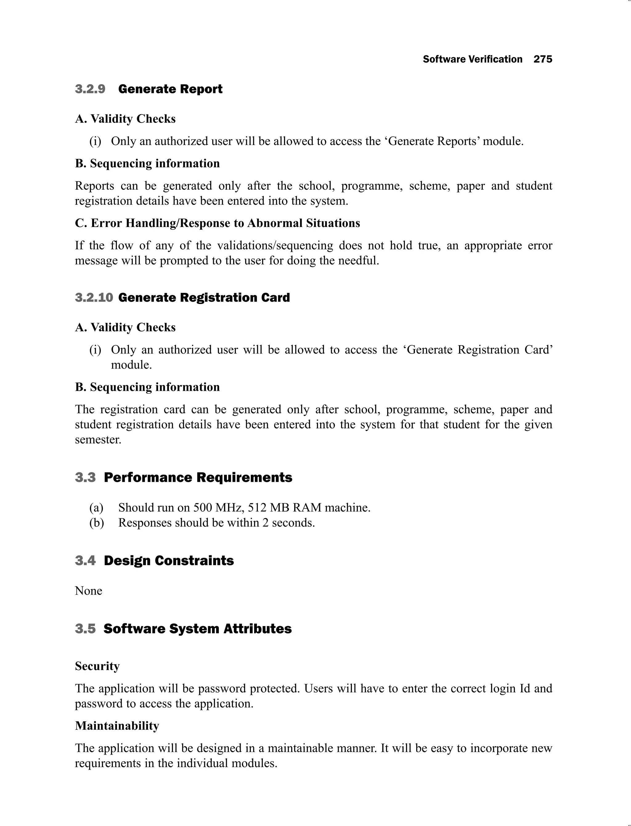
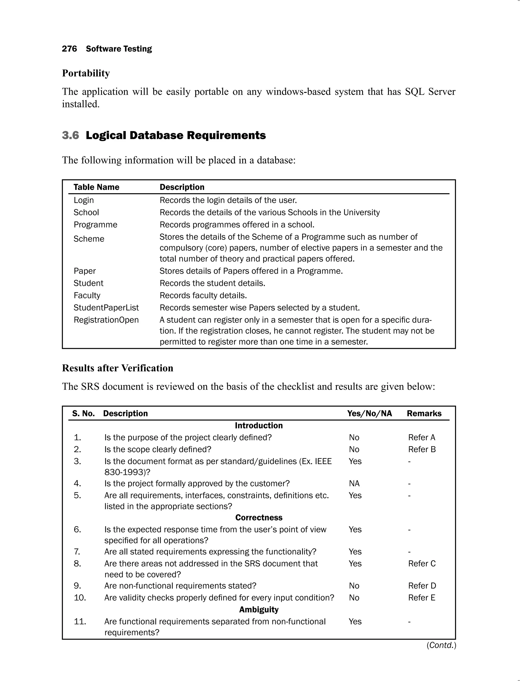
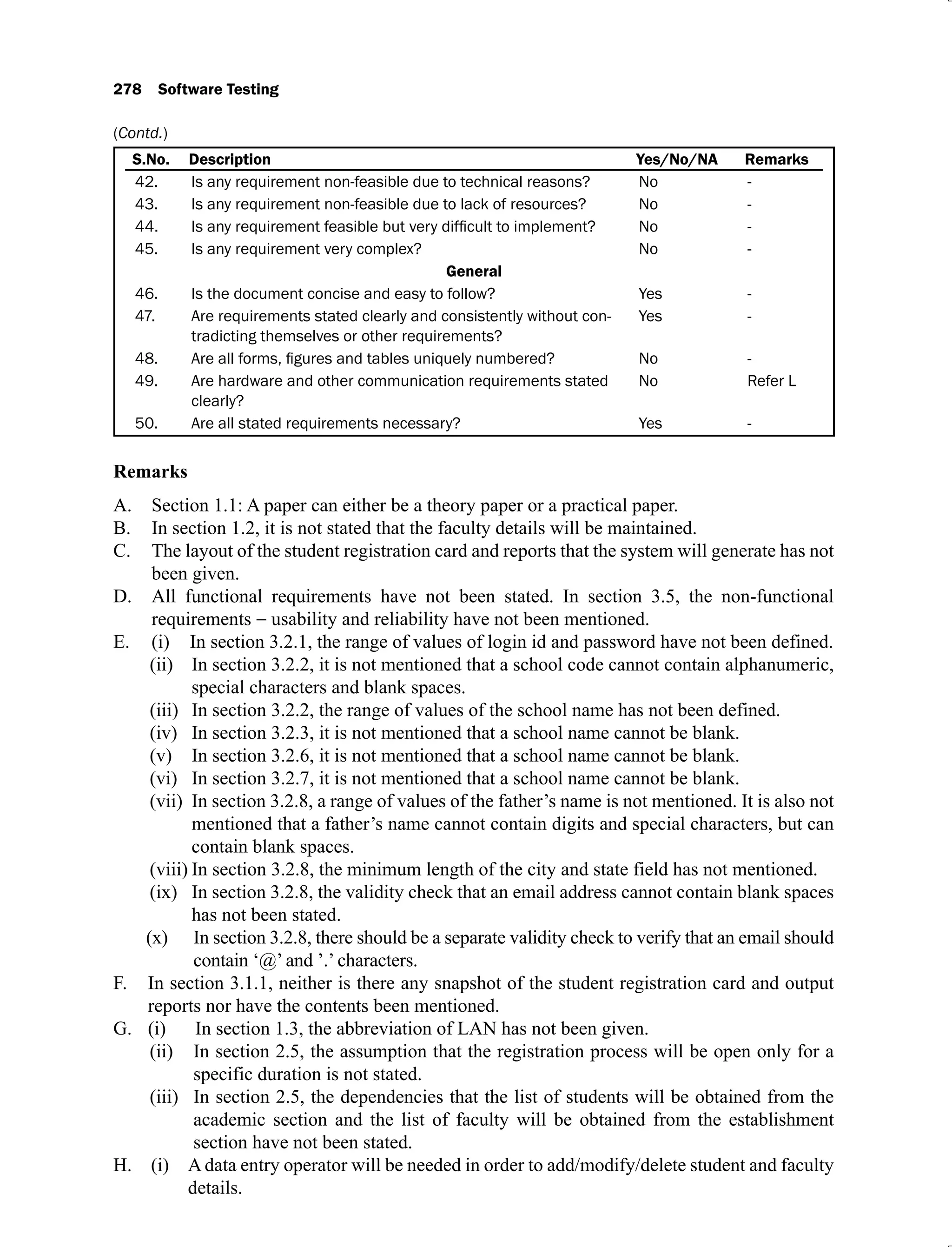
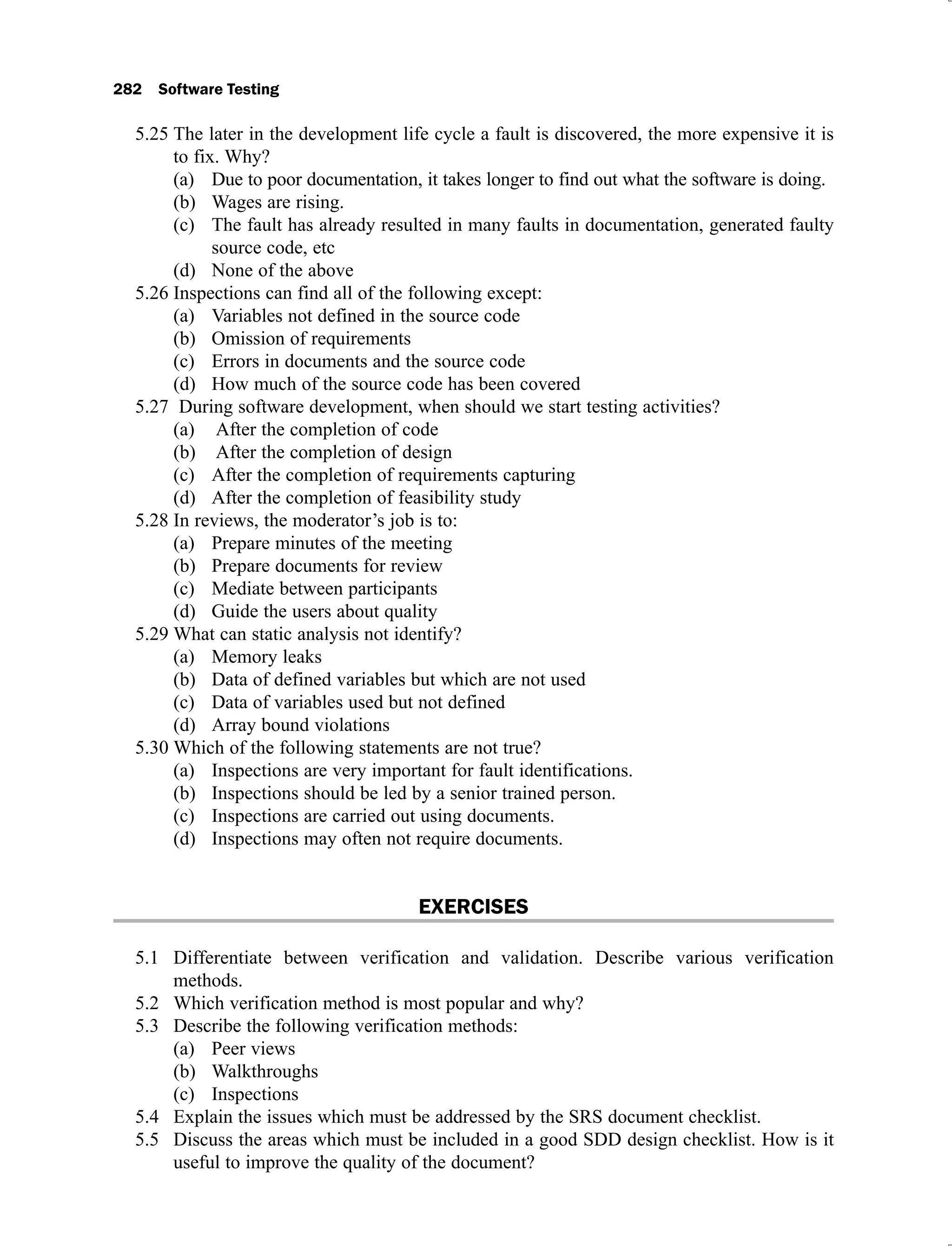
1. Customer
Provides funding, gives requirements, approves changes and
some test results.
2. Project Manager Plans and manages the project.
3. Software Developer(s)
Designs, codes and builds the software; participates in source
4. Testing co-ordinator(s)
-
ments and functional and technical documents.
5. Testing person(s) Executes the tests and documents results.
1.2.4 What Should We Test?
Is it possible to test the program for all possible valid and invalid inputs? The answer is always
negative due to a large number of inputs. We consider a simple example where a program has
two 8 bit integers as inputs. Total combinations of inputs are 28
28
. If only one second is
Introduction 17
required (possible only with automated testing) to execute one set of inputs, it may take 18
hours to test all possible combinations of inputs. Here, invalid test cases are not considered
which may also require a substantial amount of time. In practice, inputs are more than two and
the size is also more than 8 bits. What will happen when inputs are real and imaginary
numbers? We may wish to go for complete testing of the program, which is neither feasible
nor possible. This situation has made this area very challenging where the million dollar
question is, “How to choose a reasonable number of test cases out of a large pool of test
cases?” Researchers are working very hard to find the answer to this question. Many testing
techniques attempt to provide answers to this question in their own ways. However, we do not
have a standard yardstick for the selection of test cases.
We all know the importance of this area and expect some drastic solutions in the future. We
also know that every project is a new project with new expectations, conditions and constraints.
What is the bottom line for testing? At least, we may wish to touch this bottom line, which may
incorporate the following:
Execute every statement of the program at least once.
(i)
Execute all possible paths of the program at least once.
(ii)
Execute every exit of the branch statement at least once.
(iii)
This bottom line is also not easily achievable. Consider the following piece of source code:
if (x > 0)
1.
{
2.
a = a + b;
3.
}
4.
if (y>10)
5.
{
6.
c=c+d;
7.
}
8.
This code can be represented graphically as:
Line Numbers Symbol for representation
1 A
2, 3, 4 B
5 C
6, 7, 8 D
End E
18 Software Testing
The possible paths are: ACE, ABCE, ACDE and ABCDE. However, if we choose x = 9 and
y = 15, all statements are covered. Hence only one test case is sufficient for 100% statement
coverage by traversing only one path ABCDE. Therefore, 100% statement coverage may not
be sufficient, even though that may be difficult to achieve in real life programs.
Myers [MYER04] has given an example in his book entitled “The art of software testing”
which shows that the number of paths is too large to test. He considered a control flow graph
(as given in Figure 1.5) of a 10 to 20 statement program with ‘DO Loop’ that iterates up to 20
times. Within ‘DO Loop’ there are many nested ‘IF’ statements. The assumption is that all
decisions in the program are independent of each other. The number of unique paths is nothing
but the number of unique ways to move from point X to point Y. Myers further stated that
executing every statement of the program at least once may seem to be a reasonable goal.
However many portions of the program may be missed with this type of criteria.
Figure 1.5. Control flow graph of a 10 to 20 statement program [MYER04]
“The total number of paths is approximately 1014
or 100 trillion. It is computed from
520
+ 519
+ ………51
, where 5 is the number of independent paths of the control flow graph.
If we write, execute and verify a test case every five minutes, it would take approximately one
billion years to try every path. If we are 300 times faster, completing a test case one per second,
we could complete the job in 3.2 million years.” This is an extreme situation; however, in
reality, all decisions are not independent. Hence, the total paths may be less than the calculated
paths. But real programs are much more complex and larger in size. Hence, ‘testing all paths’
is very difficult if not impossible to achieve.
We may like to test a program for all possible valid and invalid inputs and furthermore, we
may also like to execute all possible paths; but practically, it is quite difficult. Every exit
condition of a branch statement is similarly difficult to test due to a large number of such
conditions. We require effective planning, strategies and sufficient resources even to target the
minimum possible bottom line. We should also check the program for very large numbers,
very small numbers, numbers that are close to each other, negative numbers, some extreme
cases, characters, special letters, symbols and some strange cases.
Introduction 19
1.3 SOME TERMINOLOGIES
Some terminologies are discussed in this section, which are inter-related and confusing but
commonly used in the area of software testing.
1.3.1 Program and Software
Both terms are used interchangeably, although they are quite different. The software is the
superset of the program(s). It consists of one or many program(s), documentation manuals and
operating procedure manuals. These components are shown in Figure 1.6.
Figure 1.6. Components of the software
The program is a combination of source code and object code. Every phase of the software
development life cycle requires preparation of a few documentation manuals which are shown
in Figure 1.7. These are very helpful for development and maintenance activities.
Figure 1.7. Documentation manuals
20 Software Testing
Operating procedure manuals consist of instructions to set up, install, use and to maintain
the software. The list of operating procedure manuals / documents is given in Figure 1.8.
Reference guide
System overview
Beginner’s guide
tutorial
Terminology and
help manual
Maintenance guide
System administration
guide
Installation guide
Figure 1.8. Operating system manuals
1.3.2 Verification and Validation
These terms are used interchangeably and some of us may also feel that both are synonyms.
The Institute of Electrical and Electronics Engineers (IEEE) has given definitions which are
largely accepted by the software testing community. Verification is related to static testing
which is performed manually. We only inspect and review the document. However, validation
is dynamic in nature and requires the execution of the program.
Verification: As per IEEE [IEEE01], “It is the process of evaluating the system or component
to determine whether the products of a given development phase satisfy the conditions imposed
at the start of that phase.” We apply verification activities from the early phases of the software
development and check / review the documents generated after the completion of each phase.
Hence, it is the process of reviewing the requirement document, design document, source code
and other related documents of the project. This is manual testing and involves only looking at
the documents in order to ensure what comes out is what we expected to get.
Validation: As per IEEE [IEEE01], “It is the process of evaluating a system or component
during or at the end of development process to determine whether it satisfies the specified
requirements.” It requires the actual execution of the program. It is dynamic testing and
requires a computer for execution of the program. Here, we experience failures and identify
the causes of such failures.
Hence, testing includes both verification and validation. Thus
Testing = Verification + Validation
Both are essential and complementary activities of software testing. If effective verification is
carried out, it may minimize the need of validation and more number of errors may be detected
in the early phases of the software development. Unfortunately, testing is primarily validation
oriented.
Introduction 21
1.3.3 Fault, Error, Bug and Failure
All terms are used interchangeably although error, mistake and defect are synonyms in software
testing terminology. When we make an error during coding, we call this a ‘bug’. Hence, error /
mistake / defect in coding is called a bug.
A fault is the representation of an error where representation is the mode of expression such
as data flow diagrams, ER diagrams, source code, use cases, etc. If fault is in the source code,
we call it a bug.
A failure is the result of execution of a fault and is dynamic in nature. When the expected
output does not match with the observed output, we experience a failure. The program has to
execute for a failure to occur. A fault may lead to many failures. A particular fault may cause
different failures depending on the inputs to the program.
1.3.4 Test, Test Case and Test Suite
Test and test case terms are synonyms and may be used interchangeably. A test case consists
of inputs given to the program and its expected outputs. Inputs may also contain pre-
condition(s) (circumstances that hold prior to test case execution), if any, and actual inputs
identified by some testing methods. Expected output may contain post-condition(s)
(circumstances after the execution of a test case), if any, and outputs which may come as a
result when selected inputs are given to the software. Every test case will have a unique
identification number. When we do testing, we set desire pre-condition(s), if any, given
selected inputs to the program and note the observed output(s). We compare the observed
output(s) with the expected output(s) and if they are the same, the test case is successful. If
they are different, that is the failure condition with selected input(s) and this should be recorded
properly in order to find the cause of failure. A good test case has a high probability of showing
a failure condition. Hence, test case designers should identify weak areas of the program and
design test cases accordingly. The template for a typical test case is given in Table 1.7.
Table 1.7. Test case template
Part I (Before Execution)
1. Purpose of test case:
2.
Pre-condition(s):
(optional)
3. Input(s) :
4. Expected Output(s) :
5. Post-condition(s) :
6. Written by :
7. Date of design :
Part II (After Execution)
1. Output(s) :
2.
Post-condition(s) :
(optional)
(Contd.)
22 Software Testing
Part II (After Execution)
3. Pass / fail :
4. If fails, any possible reason of failure (optional) :
5. Suggestions (optional)
6. Run by :
7. Date of suggestion :
The set of test cases is called a test suite. We may have a test suite of all test cases, test suite
of all successful test cases and test suite of all unsuccessful test cases. Any combination of test
cases will generate a test suite. All test suites should be preserved as we preserve source code
and other documents. They are equally valuable and useful for the purpose of maintenance of
the software. Sometimes test suite of unsuccessful test cases gives very important information
because these are the test cases which have made the program fail in the past.
1.3.5 Deliverables and Milestones
Different deliverables are generated during various phases of the software development. The
examples are source code, Software Requirements and Specification document (SRS),
Software Design Document (SDD), Installation guide, user reference manual, etc.
The milestones are the events that are used to ascertain the status of the project. For instance,
finalization of SRS is a milestone; completion of SDD is another milestone. The milestones
are essential for monitoring and planning the progress of the software development.
1.3.6 Alpha, Beta and Acceptance Testing
Customers may use the software in different and strange ways. Their involvement in testing
may help to understand their minds and may force developers to make necessary changes in
the software. These three terms are related to the customer’s involvement in testing with
different meanings.
Acceptance Testing: This term is used when the software is developed for a specific customer.
The customer is involved during acceptance testing. He/she may design adhoc test cases or
well-planned test cases and execute them to see the correctness of the software. This type of
testing is called acceptance testing and may be carried out for a few weeks or months. The
discovered errors are fixed and modified and then the software is delivered to the customer.
Alpha and Beta Testing: These terms are used when the software is developed as a product
for anonymous customers. Therefore, acceptance testing is not possible. Some potential
customers are identified to test the product. The alpha tests are conducted at the developer’s
site by the customer. These tests are conducted in a controlled environment and may start when
the formal testing process is near completion. The beta tests are conducted by potential
customers at their sites. Unlike alpha testing, the developer is not present here. It is carried out
in an uncontrolled real life environment by many potential customers. Customers are expected
to report failures, if any, to the company. These failure reports are studied by the developers
and appropriate changes are made in the software. Beta tests have shown their advantages in
the past and releasing a beta version of the software to the potential customer has become a
(Contd.)
Introduction 23
common practice. The company gets the feedback of many potential customers without
making any payment. The other good thing is that the reputation of the company is not at stake
even if many failures are encountered.
1.3.7 Quality and Reliability
Software reliability is one of the important factors of software quality. Other factors are
understandability, completeness, portability, consistency, maintainability, usability, efficiency,
etc. These quality factors are known as non-functional requirements for a software system.
Software reliability is defined as “the probability of failure free operation for a specified time
in a specified environment” [ANSI91]. Although software reliability is defined as a probabilistic
function and comes with the notion of time, it is not a direct function of time. The software does
not wear out like hardware during the software development life cycle. There is no aging concept
in software and it will change only when we intentionally change or upgrade the software.
Software quality determines how well the software is designed (quality of design), and how
well the software conforms to that design (quality of conformance).
Some software practitioners also feel that quality and reliability is the same thing. If we are
testing a program till it is stable, reliable and dependable, we are assuring a high quality
product. Unfortunately, that is not necessarily true. Reliability is just one part of quality. To
produce a good quality product, a software tester must verify and validate throughout the
software development process.
1.3.8 Testing, Quality Assurance and Quality Control
Most of us feel that these terms are similar and may be used interchangeably. This creates
confusion about the purpose of the testing team and Quality Assurance (QA) team. As we have
seen in the previous section (1.2.1), the purpose of testing is to find faults and find them in the
early phases of software development. We remove faults and ensure the correctness of removal
and also minimize the effect of change on other parts of the software.
The purpose of QA activity is to enforce standards and techniques to improve the
development process and prevent the previous faults from ever occurring. A good QA activity
enforces good software engineering practices which help to produce good quality software.
The QA group monitors and guides throughout the software development life cycle. This is a
defect prevention technique and concentrates on the process of the software development.
Examples are reviews, audits, etc.
Quality control attempts to build a software system and test it thoroughly. If failures are
experienced, it removes the cause of failures and ensures the correctness of removal. It
concentrates on specific products rather than processes as in the case of QA. This is a defect
detection and correction activity which is usually done after the completion of the software
development. An example is software testing at various levels.
1.3.9 Static and Dynamic Testing
Static testing refers to testing activities without executing the source code. All verification
activities like inspections, walkthroughs, reviews, etc. come under this category of testing.
24 Software Testing
This, if started in the early phases of the software development, gives good results at a very
reasonable cost. Dynamic testing refers to executing the source code and seeing how it
performs with specific inputs. All validation activities come in this category where execution
of the program is essential.
1.3.10 Testing and Debugging
The purpose of testing is to find faults and find them as early as possible. When we find any
such fault, the process used to determine the cause of this fault and to remove it is known as
debugging. These are related activities and are carried out sequentially.
1.4 LIMITATIONS OF TESTING
We want to test everything before giving the software to the customers. This ‘everything’ is
very illusive and has many meanings. What do we understand when we say ‘everything’? We
may expect one, two or all of the following when we refer to ‘everything’:
Execute every statement of the program
(i)
Execute every true and false condition
(ii)
Execute every condition of a decision node
(iii)
Execute every possible path
(iv)
Execute the program with all valid inputs
(v)
Execute the program with all invalid inputs
(vi)
These six objectives are impossible to achieve due to time and resource constraints as
discussed in section 1.2.4. We may achieve a few of them. If we do any compromise, we may
miss a bug. Input domain is too large to test and there are too many paths in any program.
Hence ‘Everything’ is impossible and we have to settle for ‘less than everything’ in real life
situations. Some of the other issues which further make the situation more complex and
complicated are given in the subsequent sub-sections.
1.4.1 Errors in the Software Requirement and Specification Document
These issues are very difficult to identify. If 6+9=20 is written in the SRS document and our
program prints output as 20 when 6 and 9 are inputs, is it a bug? If the program prints output
as 15, when inputs are 6 and 9, how can we interpret? In this case, the actual output is so
obvious that interpretation may not require time to take a correct decision. But in most of the
situations, outputs are not so obvious. Some requirements may be misunderstood and some
may be missed. Ambiguities of natural languages (like English) may give more than one
meaning to a sentence and make life difficult for testers. Hence, problems in writing good SRS
have also become one of the problems of software testing.
1.4.2 Logical Bugs
How do we handle logical bugs? An interesting example is given in Figure 1.9. In this function,
statement “d = c++;” given in line number 4 is incorrect. As per requirements, it should have
Introduction 25
been “d = ++c”; but due to a typographical mistake and ignorance, “d = c++;” has been written.
This is a logical error and cannot be detected by the compiler. Here, confusion is due to the use
of prefix and postfix operators. A prefix operator first adds 1 to the operand and then the result
is assigned to the variable on the left. On the other hand, a postfix operator first assigns the
value to the variable on the left and then increment the operand [BALA07]. In this function the
postfix operator is used instead of the prefix operator. The function returns the integer value of
‘flag’. If this function is executed on a 16 bit computer, the valid integer range for input ‘c’ is
–32768 to 32767. Hence, there are 65536 possible inputs to this program. We may not like to
create 65536 test cases. After all, who will execute those cases, if at all created, one fine day?
Which input values are to be selected for the detection of this bug? Ten test cases have been
given in Table 1.8 and none of them could detect this bug. How many test cases out of possible
65536 test cases will find this bug? What are the chances that we will select all those test cases
or any one of them in order to find this bug? Only two test cases out of 65536 can detect this
bug and are given in Table 1.9. This example shows the impossibility of testing ‘everything’.
If a small function can create so many problems, we may appreciate the problems of real life
large and complex programs. Logical bugs are extremely difficult to handle and become one
of the serious concerns of testing.
Software testing has inherent difficulties which is making it impossible to completely test
the software. It can only show that bugs are in the software but it cannot show that bugs are
not in the software at all. With all the limitations, software testing still is mandatory and a very
useful filter to detect errors, which may further be removed. However we all know that good
testing cannot make the software better, only good coding with software engineering principles
makes the software better. However, good testing techniques may detect a good number of
errors and their removal may improve the quality of the software.
1. int funct1 (int c)
2. {
3. int d, flag;
4. d = c ++ ; // should be d = ++ c; as per requirements
5. if (d < 20000)
6. flag = 1 ;
7. else
8. flag = 0;
9. return (flag);
10. }
Figure 1.9. A typical example
Table 1.8. Test cases for function of Figure 1.9
Test case Input c Expected output Actual output
1. 0 1 1
2. 1 1 1
3. 20000 0 0
4. 30000 0 0
(Contd.)
26 Software Testing
Test case Input c Expected output Actual output
5. –10000 1 1
6. –20000 1 1
7. –1 1 1
8. –16000 1 1
9. 27000 0 0
10. 32000 0 0
Table 1.9. Typical test cases where outputs are different
Input c Expected output Actual output
19999 0 1
32767 0
1.4.3 Difficult to Measure the Progress of Testing
How to measure the progress of testing? Normally we count various things to measure and
interpret these counts. Is experiencing more failures good news or bad news? The answer could
be either. A higher number of failures may indicate that testing was thorough and very few
faults remain in the software. Or, it may be treated as an indication of poor quality of the
software with lots of faults; even though many have been exposed, lots of them still remain.
These counts may be illusive and may not help us to measure the progress of testing.
This difficulty of measuring the progress of testing leads to another issue i.e. when to stop
testing and release the software to the customer(s)? This is a sensitive decision and should be
based on the status of testing. However, in the absence of testing standards, ‘economics’, ‘time
to market’ and ‘gut feeling’ have become important issues over technical considerations for the
release of any software. Many models are available with serious limitations and are not
universally acceptable.
Software companies are facing serious challenges in testing their products and these challenges
are growing bigger as the software grows more complex. Hence, we should recognize the
complex nature of testing and take it seriously. The gap between standards and practices should
be reduced in order to test the software effectively which may result in to good quality
software.
1.5 THE V SHAPED SOFTWARE LIFE CYCLE MODEL
The V shaped model is the modified form of the waterfall model with a special focus on testing
activities. The waterfall model allows us to start testing activities after the completion of the
implementation phase. This was popular when testing was primarily validation oriented. Now,
there is a shift in testing activities from validation to verification where we want to review /
inspect every activity of the software development life cycle. We want to involve the testing
persons from the requirement analysis and specification phase itself. They will review the SRS
document and identify the weak areas, critical areas, ambiguous areas and misrepresented
areas. This will improve the quality of the SRS document and may further minimize the errors.
(Contd.)
Introduction 27
These verification activities are treated as error preventive exercises and are applied at
requirements analysis and specification phase, high level design phase, detailed design phase
and implementation phase. We not only want to improve the quality of the end products at all
phases by reviews, inspections and walkthroughs, but also want to design test cases and test
plans during these phases. The designing of test cases after requirement analysis and
specification phase, high level design phase, detailed design phase and implementation phase
may help us to improve the quality of the final product and also reduce the cost and development
time.
1.5.1 Graphical Representation
The shape of the model is like the English letter ‘V’ and it emphasizes testing activities in
every phase. There are two parts of the software development life cycle in this model i.e.
development and testing and are shown in Figure 1.10. We want to carry out development and
testing activities in parallel and this model helps us to do the same in order to reduce time and
cost.
Figure 1.10. V shaped software development life cycle model
1.5.2 Relationship of Development and Testing Parts
The development part consists of the first four phases (i.e. requirements analysis and specification,
high level design, detailed design and implementation) whereas the testing part has three phases
(i.e. unit and integration testing, system testing and acceptance testing). The model establishes
the relationship between the development and testing parts. The acceptance test case design and
planning activities should be conducted along with the software requirements and specifications
28 Software Testing
phase. Similarly the system test case design and planning activities should be carried out along with
high level design phase. Unit and integration test case design and planning activities should be
carried out along with the detailed design phase. The development work is to be done by the
development team and testing is to be done by the testing team simultaneously.After the completion
of implementation, we will have the required test cases for every phase of testing. The only
remaining work is to execute these test cases and observe the responses of the outcome of the
execution. This model brings the quality into the development of our products. The encouragement
of writing test cases and test plans in the earlier phases of the software development life cycle is the
real strength of this model. We require more resources to implement this model as compared to the
waterfall model. This model also suffers from many disadvantages of the waterfall model like non-
availabilityofaworkingversionoftheproductuntillateinthelifecycle,difficultyinaccommodating
any change, etc. This model has also limited applications in today’s interactive software
processes.
MULTIPLE CHOICE QUESTIONS
Note: Select the most appropriate answer for the following questions.
What is software testing?
1.1
It is the process of demonstrating that errors are not present.
(a)
It is the process of establishing confidence that a program does what it is supposed
(b)
to do.
It is the process of executing a program with the intent of finding errors.
(c)
It is the process of showing the correctness of a program.
(d)
Why should testing be done?
1.2
To ensure the correctness of a program
(a)
To find errors in a program
(b)
To establish the reliability of a program
(c)
To certify the effectiveness of a program
(d)
Which phase consumes maximum effort to fix an error?
1.3
Requirements analysis and specifications
(a)
Design phase
(b)
Coding phase
(c)
Feasibility study phase
(d)
Which objective is most difficult to achieve?
1.4
Execute every statement of a program at least once
(a)
Execute every branch statement of a program at least once
(b)
Execute every path of a program at least once
(c)
Execute every condition of a branch statement of a program at least once
(d)
Software errors during coding are known as:
1.5
Bugs
(a)
Defects
(b)
Failures
(c)
Mistakes
(d)
Introduction 29
The cost of fixing an error is:
1.6
More in requirements analysis and specification phase than coding phase
(a)
More in coding phase than requirements analysis and specification phase
(b)
Same in all phases of a software development life cycle
(c)
Negligible in all phases
(d)
Beta testing is done by:
1.7
Developers
(a)
Testers
(b)
Potential customers
(c)
Requirements writers
(d)
Alpha testing is carried out at the:
1.8
Developer’s site in a controlled environment
(a)
Developer’s site in a free environment
(b)
Customer’s site in a controlled environment
(c)
Customer’s site in a free environment
(d)
The purpose of acceptance testing is:
1.9
To perform testing from the business perspective
(a)
To find faults in the software
(b)
To test the software with associated hardware
(c)
To perform feasibility study
(d)
Acceptance testing is done by:
1.10
Developers
(a)
Customers
(b)
Testers
(c)
All of the above
(d)
Program is:
1.11
Subset of software
(a)
Superset of software
(b)
Set of software
(c)
Union of software
(d)
Which is not an infrastructure software?
1.12
Compiler
(a)
Operating system
(b)
Testing tools
(c)
Result Management Software
(d)
Software should have:
1.13
Program + operating system + compiler
(a)
Set of programs + operating system
(b)
Programs + documentation + operating procedures
(c)
None of the above
(d)
Concepts of software testing are applicable to:
1.14
Procedural programming languages
(a)
Object oriented programming languages
(b)
‘C’, ‘C++’ and Java programming languages
(c)
All of the abo
(d) ve
30 Software Testing
CASE Tool is:
1.15
Computer Aided Software Engineering Tool
(a)
Component Aided Software Engineering Tool
(b)
Constructive Aided Software Engineering Tool
(c)
Complete Analysis Software Enterprise Tool
(d)
One fault may lead to:
1.16
One failure
(a)
Many failures
(b)
No failure
(c)
All of the above
(d)
Test suite of a program is a:
1.17
Set of test cases
(a)
Set of inputs with pre-conditions
(b)
Set of outputs with post-conditions
(c)
Set of testing strategies
(d)
Alpha and Beta testing techniques are related to:
1.18
Unit testing
(a)
Integration testing
(b)
System testing
(c)
Testing by Customer
(d)
Testing a software is primarily focused on:
1.19
Verification activities only
(a)
Validation activities only
(b)
Verification and validation activities
(c)
None of the above
(d)
Testing a software with real data in real environment is known as:
1.20
Alpha testing
(a)
Beta testing
(b)
System testing
(c)
Integration testing
(d)
Verification activities are:
1.21
Performed manually
(a)
Related to reviewing the documents and source code
(b)
Known as static testing
(c)
All of the above
(d)
Validation activities are:
1.22
Dynamic activities and require program execution
(a)
Related to inspecting the source code
(b)
Related to static testing
(c)
Related to source code design and documentation
(d)
When the output of a program is different from the expected output, it is known as:
1.23
A fault
(a)
An error
(b)
A failure
(c)
A mistake
(d)
Introduction 31
Software testing activities should be started:
1.24
After the completion of source code
(a)
After the completion of design phase
(b)
As early as possible in the software development life cycle
(c)
After the completion of software requirements and analysis phase
(d)
Software testing activities are important in:
1.25
Every phase of the software development life cycle
(a)
The last few phases of the software development life cycle
(b)
The software requirements and analysis phase
(c)
All of the above
(d)
The focus of acceptance testing is:
1.26
To find faults
(a)
To ensure correctness of software
(b)
To test integration related issues
(c)
To test from the user’s perspective
(d)
A reliable software is one which is:
1.27
Liked by its users
(a)
Delivered on time and with budget
(b)
Unlikely to cause failures
(c)
Very easy to use
(d)
When to stop testing and release the software to customers should be decided on the basis
1.28
of:
Market conditions
(a)
Budget and availability of resources
(b)
Test metrics
(c)
Capabilities of the testing persons
(d)
What are the good software testing practices?
1.29
Involve testing persons as early as possible in the software development life
(a)
cycle
Apply effective verification techniques
(b)
Enforce inspections and reviews after every phase of the software development
(c)
life cycle
All of the above
(d)
What is a test case?
1.30
Input(s), expected output(s), pre-condition(s) and post-condition(s)
(a)
Steps of execution
(b)
A list of activities which can be tested
(c)
None of the above
(d)
You cannot control what you cannot :
1.31
Define
(a)
Measure
(b)
Improve
(c)
Change
(d)
What is the major benefit of verifications in the early phases of the software development
1.32
life cycle?
32 Software Testing
It identifies changes in the SRS
(a)
It reduces defect multiplication
(b)
It allows involvement of testing persons
(c)
It improves discipline in the various development activities
(d)
Behavioural specifications are required for:
1.33
Modelling
(a)
Verification
(b)
Validation
(c)
Testing
(d)
Which, in general, is the least expected skill of a testing person?
1.34
Diplomatic
(a)
Reliable
(b)
Having good attention to detail
(c)
Good developer
(d)
Debugging of a program is
1.35
The process of executing the program
(a)
The process of identifying a fault and removing it from the program
(b)
The process of experiencing a failure
(c)
The process of improving the quality of the program
(d)
All validation activities come under the category of:
1.36
Dynamic testing
(a)
Static testing
(b)
Source code design
(c)
None of the above
(d)
All verification activities come under the category of:
1.37
Dynamic testing
(a)
Static testing
(b)
Source code design
(c)
None of the above
(d)
Which is not a factor of software quality?
1.38
Reliability
(a)
Portability
(b)
Efficiency
(c)
Functionality
(d)
Which is the most important factor of software quality?
1.39
Reliability
(a)
Understandability
(b)
Efficiency
(c)
Consistency
(d)
Quality assurance activities concentrate on
1.40
Software design
(a)
Software performance
(b)
Software products
(c)
Software processes
(d)
Which is not the quality of a testing person?
1.41
Introduction 33
Cautious
(a)
Curious
(b)
Judgmental
(c)
Critical
(d)
What should be the best possible objective for testing?
1.42
Execute every statement at least once
(a)
Execute every path at least once
(b)
Execute every branch statement at least once
(c)
Execute every condition of a branch statement at least once
(d)
Which is not a user manual?
1.43
Reference guide
(a)
Beginner’s guide
(b)
Sequence diagrams
(c)
System overview
(d)
Which is not a documentation manual?
1.44
SRS document
(a)
SDD document
(b)
Source code
(c)
Installation guide
(d)
Which is not the limitation of testing?
1.45
Difficult to measure the progress of testing
(a)
Availability of testing tools
(b)
Input domain is too large to test
(c)
Too many paths in the program
(d)
How much percentage of cost is generally consumed in software testing with reference
1.46
to software development cost?
10 – 20
(a)
40 – 50
(b)
80 – 90
(c)
70 – 80
(d)
How much testing is enough?
1.47
Not easy to decide
(a)
Depends on complexity and criticality
(b)
Depends on abilities of testing persons
(c)
Depends on maturity of developers
(d)
If an expected output is not specified then:
1.48
We cannot execute the test case
(a)
We may not be able to repeat the test
(b)
We may not be able to decide if the test has passed or failed
(c)
We may not be able to automate the testing activity
(d)
Which of the following is a reason for a software failure?
1.49
Testing fault
(a)
Software Fault
(b)
Design Fault
(c)
Requirement Fault
(d)
34 Software Testing
Why is it impossible to test a program completely?
1.50
Input domain is too large to test
(a)
Good testers are not available
(b)
Efficient testing tools are not available
(c)
None of the above
(d)
EXERCISES
What is software testing? Is it possible to do complete testing?
1.1
What are the limitations of testing? Discuss with the help of examples.
1.2
Describe some software failures. How can we minimize such failures?
1.3
Why should we test software? What are the associated risks, if we release it without
1.4
testing?
Who should do the testing of the software? Is there any international standard?
1.5
What should we test? Discuss the areas which should be focused on during testing.
1.6
There are two limitations in software testing:
1.7
Input domain is too large to test
(i)
Too many paths in the program
(ii)
Justify these limitations with the help of suitable examples.
What are logical bugs? How are they different from syntax bugs? How can we handle
1.8
logical bugs effectively?
Write a program to add two digit integers. Can we test the program completely? If so,
1.9
how many test cases are required? Assume that each test case can be executed and
analyzed in one second; how long would it take to execute all test cases?
What is the testing process? How can it be implemented? What are its limitations?
1.10
Will exhaustive testing (even if possible for a very small program) guarantee that the
1.11
program is 100% correct?
What are the objectives of testing? Why is the psychology of the testing person impo-
1.12
rtant?
Software does not break or wear out with time (unlike hardware). Why does software
1.13
fail even after a good amount of testing?
What is the tester’s role in software development?
1.14
When to stop testing is a very crucial decision. What factors should be considered for
1.15
taking such a decision?
Differentiate between
1.16
Alpha and Beta testing
(i)
Development and regression testing
(ii)
Fault, bug and failure
(iii)
Verification and validation
(iv)
Static and dynamic testing
(v)
Program and software
(vi)
Test, Test case and Test Suite
(vii)
Deliverable and milestones
(viii)
Quality and Reliability
(ix)
Testing, Quality Assurance and Quality Control
(x)
Introduction 35
Explain a typical test case template. What are the reasons for documenting test cases?
1.17
With the help of a suitable example, illustrate why exhaustive testing is not possible.
1.18
Define a test case. What are the objectives of test case design? Discuss the various
1.19
steps involved.
What is the role of Quality Assurance in software development? How is it different
1.20
from Quality Control?
What is software crisis? Was Y2K a software crisis?
1.21
What are the components of a software system? Discuss how a software differs from
1.22
a program.
Differentiate between generic and customized software products. Which one has a
1.23
large market share and why?
What is a software failure? Discuss the conditions of a failure. Mere presence of faults
1.24
may not lead to failures. Explain with the help of an example.
Verification and validation are used interchangeably many times. Define these terms
1.25
and establish their relationship with testing.
Testing is not a single phase in the software development life cycle. Explain and
1.26
comment.
Discuss the advantages of testing with reference to the software product.
1.27
Discuss the significance of the V-shaped software life cycle model and also establish
1.28
the relationship between its development and testing parts.
What is the relationship of the V-shaped software life cycle model with the waterfall
1.29
model? How is acceptance testing related to requirement analysis and specification
phase?
Differentiate between the V-shaped software life cycle model and the waterfall model.
1.30
FURTHER READING
The classic book on software testing which was the only book of note for years is:
G.J. Myers, “The Art of Software Testing”, John Wiley and Sons, Inc., 1977.
One of the first articles that describes the changes in growth of software testing is:
D. Gelperin, B. Hetzel, “The Growth of Software Testing”, Communications of
the ACM, vol. 31, no. 6, June 1988.
Read the record report of Prof. J.L. Lions, Chairman Inquiry Board and Director
General of ESA prepared on 19th July, 1996 for Identification of the Causes of Failure
of Ariane 5:
J.L. Lions, “Ariane 5 Flight 501 Failure”, http://esamultimedia.esa.int/docs/esa-
x-1819eng.pdf, July 19, Paris, 1996.
Many good books and articles have been written on the causes of software failure,
including:
S.A. Sherer, ‘Software Failure Risk”, Plenum, 1992.
P. Neumann, “Computer Related Risks”, Addison Wesley, 1995.
S. Flowers, “Software Failure: Management Failure”, John Wiley and Sons,
1996.
36 Software Testing
C. Jones, “Patterns of Software Systems Failure and Success”, International
Thomson Computer Press, 1996.
Ron Patton, “Software Testing”, Techmedia, Delhi, India, 2002.
K. Ewusi-Mensah’s, “Software Development Failures”, MIT Press, 2003.
R.N. Charette, “Why Software Fails?”, IEEE Spectrum, September 2005.
A very good article that shows why removing bugs is difficult and why testing is a
constant challenge may be found in:
J A. Whittaker, “What Is Software Testing? And Why Is It So Hard?”, IEEE
Software, January/February, 2000.
An interesting article of Mann about bugs of Windows XP may be found at:
Charles C. Mann, “Why Software is so bad”, Technology Review, www.techno-
logyreview.com, 2002.
The report presented by RTI for the U.S. Department of Commerce’s National Institute
of Standards and Technology (NIST) is a very good study that quantifies the problem
of software errors. The study states “Software errors cost U.S. economy $59.5 billion
annually.” The detailed report can be found at:
www.nist.gov/public_affairs/update/upd20020624.htm#Economics
M.P. Gallaher and B.M. Kropp, “Economic Impacts of Inadequate Infrastructure
for Software Testing”, NSIT Report, May 2002.
Some of the useful facts about software may be found in:
R. L. Glass, “Facts and Fallacies of Software Engineering”, Pearson Education,
2003.
Further list of software failures may be read from:
http://www.sereferences.com/software-failure-list.php
Aconcise list of 28 best practices for software testing arranged in order of implementation
is summarized in:
R. Chillarege, “Software Testing Best Practices”, IBM Research Technical Report,
1999.
Bret Pettichord’s Software testing hotlist can be checked from:
http://www.io.com/~wazmo/qa/
The online Forum on “Risks to the Public in Computers and Related Systems” is
available at http://catless.ncl.ac.uk/risks.
2
Functional Testing
Software testing is very important but is an effort-consuming activity. A large number of test
cases are possible and some of them may make the software fail. As we all know, if observed
behaviour of the software is different from the expected behaviour, we treat this as a failure
condition. Failure is a dynamic condition that always occurs after the execution of the software.
Everyone is in search of such test cases which may make the software fail and every technique
attempts to find ways to design those test cases which have a higher probability of showing a
failure.
Functional testing techniques attempt to design those test cases which have a higher probability
of making a software fail. These techniques also attempt to test every possible functionality of
the software. Test cases are designed on the basis of functionality and the internal structure of the
program is completely ignored. Observed output(s) is (are) compared with expected output(s) for
selected input(s) with preconditions, if any. The software is treated as a black box and therefore,
it is also known as black box testing as shown in Figure 2.1.
Figure 2.1. Functional (Black Box) testing
Every dot in the input domain represents a set of inputs and every dot in the output domain
represents a set of outputs. Every set of input(s) will have a corresponding set of output(s). The
test cases are designed on the basis of user requirements without considering the internal
structure of the program. This black box knowledge is sufficient to design a good number of
test cases. Many activities are performed in real life with only black box knowledge like
38 Software Testing
driving a car, using a cell phone, operating a computer, etc. In functional testing techniques,
execution of a program is essential and hence these testing techniques come under the category
of ‘validation’. Here, both valid and invalid inputs are chosen to see the observed behaviour of
the program. These techniques can be used at all levels of software testing like unit, integration,
system and acceptance testing. They also help the tester to design efficient and effective test
cases to find faults in the software.
2.1 BOUNDARY VALUE ANALYSIS
This is a simple but popular functional testing technique. Here, we concentrate on input values
and design test cases with input values that are on or close to boundary values. Experience has
shown that such test cases have a higher probability of detecting a fault in the software.
Suppose there is a program ‘Square’ which takes ‘x’ as an input and prints the square of ‘x’as
output. The range of ‘x’ is from 1 to 100. One possibility is to give all values from 1 to 100
one by one to the program and see the observed behaviour. We have to execute this program
100 times to check every input value. In boundary value analysis, we select values on or close
to boundaries and all input values may have one of the following:
Minimum value
(i)
Just above minimum value
(ii)
Maximum value
(iii)
Just below maximum value
(iv)
Nominal (Average) value
(v)
These values are shown in Figure 2.2 for the program ‘Square’.
Figure 2.2. Five values for input ‘x’ of ‘Square’ program
These five values (1, 2, 50, 99 and 100) are selected on the basis of boundary value analysis
and give reasonable confidence about the correctness of the program. There is no need to select
all 100 inputs and execute the program one by one for all 100 inputs. The number of inputs
selected by this technique is 4n + 1 where ‘n’ is the number of inputs. One nominal value is
selected which may represent all values which are neither close to boundary nor on the
boundary. Test cases for ‘Square’ program are given in Table 2.1.
Table 2.1. Test cases for the ‘Square’ program
Test Case Input x Expected output
1. 1 1
2. 2 4
3. 50 2500
4. 99 9801
5. 100 10000
Functional Testing 39
Consider a program ‘Addition’ with two input values x and y and it gives the addition of x
and y as an output. The range of both input values are given as:
100 x 300
200 y 400
The selected values for x and y are given in Figure 2.3.
Figure 2.3. Selected values for input values x and y
The ‘x’ and ‘y’ inputs are required for the execution of the program. The input domain of
this program ‘Addition’ is shown in Figure 2.4. Any point within the inner rectangle is a
legitimate input to the program.
Figure 2.4. Valid input domain for the program ‘Addition’
We also consider ‘single fault’ assumption theory of reliability which says that failures are
rarely the result of the simultaneous occurrence of two (or more) faults. Normally, one fault is
responsible for one failure. With this theory in mind, we select one input value on boundary
(minimum), just above boundary (minimum +
), just below boundary (maximum –
), on boundary
40 Software Testing
(maximum), nominal (average) and other n-1 input values as nominal values. The inputs are
shown graphically in Figure 2.5 and the test cases for ‘Addition’ program are given in Table
2.2.
Figure 2.5. Graphical representation of inputs
Table 2.2. Test cases for the program ‘Addition’
Test Case x y Expected Output
1. 100 300 400
2. 101 300 401
3. 200 300 500
4. 299 300 599
5. 300 300 600
6. 200 200 400
7. 200 201 401
8. 200 300 500
9. 200 399 599
10. 200 400 600
In Table 2.2, two test cases are common (3 and 8), hence one must be selected. This
technique generates 9 test cases where all inputs have valid values. Each dot of the Figure 2.5
represents a test case and inner rectangle is the domain of legitimate input values. Thus, for a
program of ‘n’ variables, boundary value analysis yields 4n + 1 test cases.
Example 2.1: Consider a program for the determination of the largest amongst three numbers.
Its input is a triple of positive integers (say x,y and z) and values are from interval [1, 300].
Design the boundary value test cases.
Functional Testing 41
Solution: The boundary value test cases are given in Table 2.3.
Table 2.3.
Test Case x y z Expected output
1. 1 150 150 150
2. 2 150 150 150
3. 150 150 150 150
4. 299 150 150 299
5. 300 150 150 300
6. 150 1 150 150
7. 150 2 150 150
8. 150 299 150 299
9. 150 300 150 300
10. 150 150 1 150
11. 150 150 2 150
12. 150 150 299 299
13. 150 150 300 300
Example 2.2: Consider a program for the determination of division of a student based on the
marks in three subjects. Its input is a triple of positive integers (say mark1, mark2, and mark3)
and values are from interval [0, 100].
The division is calculated according to the following rules:
Marks Obtained Division
(Average)
75 – 100 First Division with distinction
60 – 74 First division
50 – 59 Second division
40 – 49 Third division
0 – 39 Fail
Total marks obtained are the average of marks obtained in the three subjects i.e.
Average = (mark1 + mark 2 + mark3) / 3
The program output may have one of the following words:
[Fail, Third Division, Second Division, First Division, First Division with Distinction]
Design the boundary value test cases.
Solution: The boundary value test cases are given in Table 2.4.
Table 2.4. Boundary value test cases for the program determining the division of a student
Test Case mark1 mark2 mark3 Expected Output
1. 0 50 50 Fail
2. 1 50 50 Fail
3. 50 50 50 Second Division
4. 99 50 50 First Division
5. 100 50 50 First Division
(Contd.)
42 Software Testing
Test Case mark1 mark2 mark3 Expected Output
6. 50 0 50 Fail
7. 50 1 50 Fail
8. 50 99 50 First Division
9. 50 100 50 First Division
10. 50 50 0 Fail
11. 50 50 1 Fail
12. 50 50 99 First Division
13. 50 50 100 First Division
Example 2.3: Consider a program for classification of a triangle. Its input is a triple of
positive integers (say a, b, c) and the input parameters are greater than zero and less than or
equal to 100.
The triangle is classified according to the following rules:
Right angled triangle: c2
= a2
+ b2
or a2
= b2
+ c2
or b2
= c2
+ a2
Obtuse angled triangle: c2
> a2
+ b2
or a2
> b2
+ c2
or b2
> c2
+ a2
Acute angled triangle: c2
< a2
+ b2
and a2
< b2
+ c2
and b2
< c2
+ a2
The program output may have one of the following words:
[Acute angled triangle, Obtuse angled triangle, Right angled triangle, Invalid triangle]
Design the boundary value test cases.
Solution: The boundary value analysis test cases are given in Table 2.5.
Table 2.5.
Test Case a b c Expected Output
1. 1 50 50 Acute angled triangle
2. 2 50 50 Acute angled triangle
3. 50 50 50 Acute angled triangle
4. 99 50 50 Obtuse angled triangle
5. 100 50 50 Invalid triangle
6. 50 1 50 Acute angled triangle
7. 50 2 50 Acute angled triangle
8. 50 99 50 Obtuse angled triangle
9. 50 100 50 Invalid triangle
10. 50 50 1 Acute angled triangle
11. 50 50 2 Acute angled triangle
12. 50 50 99 Obtuse angled triangle
13. 50 50 100 Invalid triangle
Example 2.4: Consider a program for determining the day of the week. Its input is a triple of
day, month and year with the values in the range
(Contd.)
Functional Testing 43
1 month 12
1 day 31
1900 year 2058
The possible outputs would be the day of the week or invalid date. Design the boundary
value test cases.
Solution: The boundary value test cases are given in Table 2.6.
Table 2.6. Boundary value test cases for the program determining the day of the week
Test Case month day year Expected Output
1. 1 15 1979 Monday
2. 2 15 1979 Thursday
3. 6 15 1979 Friday
4. 11 15 1979 Thursday
5. 12 15 1979 Saturday
6. 6 1 1979 Friday
7. 6 2 1979 Saturday
8. 6 30 1979 Saturday
9. 6 31 1979 Invalid Date
10. 6 15 1900 Friday
11. 6 15 1901 Saturday
12. 6 15 2057 Friday
13. 6 15 2058 Saturday
2.1.1 Robustness Testing
This is the extension of boundary value analysis. Here, we also select invalid values and see
the responses of the program. Invalid values are also important to check the behaviour of the
program. Hence, two additional states are added i.e. just below minimum value (minimum
value –
) and just above maximum value (maximum value +
). We want to go beyond the
legitimate domain of input values. This extended form of boundary value analysis is known as
robustness testing. The inputs are shown graphically in Figure 2.6 and the test cases for the
program ‘Addition’ are given in Table 2.7. There are four additional test cases which are
outside the legitimate input domain. Thus, the total test cases in robustness testing are 6n + 1,
where ‘n’ is the number of input values. All input values may have one of the following
values:
Minimum value
(i)
Just above minimum value
(ii)
Just below minimum value
(iii)
Just above maximum value
(iv)
Just below maximum value
(v)
Maximum value
(vi)
Nominal (Average) value
(vii)
44 Software Testing
Figure 2.6. Graphical representation of inputs
Table 2.7.
Test Case x y Expected Output
1. 99 300 Invalid Input
2. 100 300 400
3. 101 300 401
4. 200 300 500
5. 299 300 599
6. 300 300 600
7. 301 300 Invalid Input
8. 200 199 Invalid Input
9. 200 200 400
10. 200 201 401
11. 200 399 599
12. 200 400 600
13. 200 401 Invalid Input
2.1.2 Worst-Case Testing
This is a special form of boundary value analysis where we don’t consider the ‘single fault’
assumption theory of reliability. Now, failures are also due to occurrence of more than one
fault simultaneously. The implication of this concept in boundary value analysis is that all
input values may have one of the following:
Minimum value
(i)
Just above minimum value
(ii)
Functional Testing 45
Just below maximum value
(iii)
Maximum value
(iv)
Nominal (Average) value
(v)
The restriction of one input value at any of the above mentioned values and other input
values must be at nominal is not valid in worst-case testing. This will increase the number of
test cases from 4n + 1 test cases to 5n
test cases, where ‘n’ is the number of input values. The
inputs for ‘Addition’ program are shown graphically in Figure 2.7. The program ‘Addition’
will have 52
= 25 test cases and these test cases are given in Table 2.8.
Figure 2.7. Graphical representation of inputs
Table 2.8. Worst test cases for the program ‘Addition’
Test Case x y Expected Output
1. 100 200 300
2. 100 201 301
3. 100 300 400
4. 100 399 499
5. 100 400 500
6. 101 200 301
7. 101 201 302
8. 101 300 401
9. 101 399 500
10. 101 400 501
11. 200 200 400
12. 200 201 401
13. 200 300 500
14. 200 399 599
(Contd.)
46 Software Testing
Test Case x y Expected Output
15. 200 400 600
16. 299 200 499
17. 299 201 500
18. 299 300 599
19. 299 399 698
20. 299 400 699
21. 300 200 500
22. 300 201 501
23. 300 300 600
24. 300 399 699
25. 300 400 700
This is a more comprehensive technique and boundary value test cases are proper sub-sets
of worst case test cases. This requires more effort and is recommended in situations where
failure of the program is extremely critical and costly [JORG07].
2.1.3 Robust Worst-Case Testing
In robustness testing, we add two more states i.e. just below minimum value (minimum value–
)
and just above maximum value (maximum value+
). We also give invalid inputs and observe
the behaviour of the program. A program should be able to handle invalid input values,
otherwise it may fail and give unexpected output values. There are seven states (minimum -
,
minimum, minimum +
, nominal, maximum –
, maximum, maximum +
) and a total of 7n
test
cases will be generated. This will be the largest set of test cases and requires the maximum
effort to generate such test cases. The inputs for the program ‘Addition’ are graphically shown
in Figure 2.8. The program ‘Addition’ will have 72
= 49 test cases and these test cases are
shown in Table 2.9.
Figure 2.8. Graphical representation of inputs
(Contd.)
Functional Testing 47
Table 2.9.
Test Case x y Expected Output
1. 99 199 Invalid input
2. 99 200 Invalid input
3. 99 201 Invalid input
4. 99 300 Invalid input
5. 99 399 Invalid input
6. 99 400 Invalid input
7. 99 401 Invalid input
8. 100 199 Invalid input
9. 100 200 300
10. 100 201 301
11. 100 300 400
12. 100 399 499
13. 100 400 500
14. 100 401 Invalid input
15. 101 199 Invalid input
16. 101 200 301
17. 101 201 302
18. 101 300 401
19. 101 399 500
20. 101 400 501
21. 101 401 Invalid input
22. 200 199 Invalid input
23. 200 200 400
24. 200 201 401
25. 200 300 500
26. 200 399 599
27. 200 400 600
28. 200 401 Invalid input
29. 299 199 Invalid input
30. 299 200 499
31. 299 201 500
32. 299 300 599
33. 299 399 698
34. 299 400 699
35. 299 401 Invalid input
36. 300 199 Invalid input
37. 300 200 500
38. 300 201 501
39. 300 300 600
40. 300 399 699
41. 300 400 700
42. 300 401 Invalid input
43. 301 199 Invalid input
44. 301 200 Invalid input
45. 301 201 Invalid input
46. 301 300 Invalid input
47. 301 399 Invalid input
48. 301 400 Invalid input
49. 301 401 Invalid input
48 Software Testing
2.1.4 Applicability
Boundary value analysis is a simple technique and may prove to be effective when used
correctly. Here, input values should be independent which restricts its applicability in many
programs. This technique does not make sense for Boolean variables where input values are
TRUE and FALSE only, and no choice is available for nominal values, just above boundary
values, just below boundary values, etc. This technique can significantly reduce the number of
test cases and is suited to programs in which input values are within ranges or within sets. This
is equally applicable at the unit, integration, system and acceptance test levels. All we want is
input values where boundaries can be identified from the requirements.
Example 2.5: Consider the program for the determination of the largest amongst three
numbers as explained in example 2.1. Design the robust test cases and worst case test cases for
this program.
Solution: The robust test cases and worst test cases are given in Table 2.10 and Table 2.11
respectively.
Table 2.10.
Test Case x y z Expected output
1. 0 150 150 Invalid input
2. 1 150 150 150
3. 2 150 150 150
4. 150 150 150 150
5. 299 150 150 299
6. 300 150 150 300
7. 301 150 150 Invalid input
8. 150 0 150 Invalid input
9. 150 1 150 150
10. 150 2 150 150
11. 150 299 150 299
12. 150 300 150 300
13. 150 301 150 Invalid input
14. 150 150 0 Invalid input
15. 150 150 1 150
16. 150 150 2 150
17. 150 150 299 299
18. 150 150 300 300
19. 150 150 301 Invalid input
Table 2.11.
Test Case x y z Expected output
1. 1 1 1 1
2. 1 1 2 2
3. 1 1 150 150
(Contd.)
Functional Testing 49
Test Case x y z Expected output
4. 1 1 299 299
5. 1 1 300 300
6. 1 2 1 2
7. 1 2 2 2
8. 1 2 150 150
9. 1 2 299 299
10. 1 2 300 300
11. 1 150 1 150
12. 1 150 2 150
13. 1 150 150 150
14. 1 150 299 299
15. 1 150 300 300
16. 1 299 1 299
17. 1 299 2 299
18. 1 299 150 299
19. 1 299 299 299
20. 1 299 300 300
21. 1 300 1 300
22. 1 300 2 300
23. 1 300 150 300
24. 1 300 299 300
25. 1 300 300 300
26. 2 1 1 2
27. 2 1 2 2
28. 2 1 150 150
29. 2 1 299 299
30. 2 1 300 300
31. 2 2 1 2
32. 2 2 2 2
33. 2 2 150 150
34. 2 2 299 299
35. 2 2 300 300
36. 2 150 1 150
37. 2 150 2 150
38. 2 150 150 150
39. 2 150 299 299
40. 2 150 300 300
41. 2 299 1 299
42. 2 299 2 299
43. 2 299 150 299
44. 2 299 299 299
45. 2 299 300 300
46. 2 300 1 300
47. 2 300 2 300
48. 2 300 150 300
49. 2 300 299 300
(Contd.)
(Contd.)
50 Software Testing
Test Case x y z Expected output
50. 2 300 300 300
51. 150 1 1 150
52. 150 1 2 150
53. 150 1 150 150
54. 150 1 299 299
55. 150 1 300 300
56. 150 2 1 150
57. 150 2 2 150
58. 150 2 150 150
59. 150 2 299 299
60. 150 2 300 300
61. 150 150 1 150
62. 150 150 2 150
63. 150 150 150 150
64. 150 150 299 299
65. 150 150 300 300
66. 150 299 1 299
67. 150 299 2 299
68. 150 299 150 299
69. 150 299 299 299
70. 150 299 300 300
71. 150 300 1 300
72. 150 300 2 300
73. 150 300 150 300
74. 150 300 299 300
75. 150 300 300 300
76. 299 1 1 299
77. 299 1 2 299
78. 299 1 150 299
79. 299 1 299 299
80. 299 1 300 300
81. 299 2 1 299
82. 299 2 2 299
83. 299 2 150 299
84. 299 2 299 299
85. 299 2 300 300
86. 299 150 1 299
87. 299 150 2 299
88. 299 150 150 299
89. 299 150 299 299
90. 299 150 300 300
91. 299 299 1 299
92. 299 299 2 299
93. 299 299 150 299
94. 299 299 299 299
95. 299 299 300 300
(Contd.)
(Contd.)
Functional Testing 51
Test Case x y z Expected output
96. 299 300 1 300
97. 299 300 2 300
98. 299 300 150 300
99. 299 300 299 300
100. 299 300 300 300
101. 300 1 1 300
102. 300 1 2 300
103. 300 1 150 300
104. 300 1 299 300
105. 300 1 300 300
106. 300 2 1 300
107. 300 2 2 300
108. 300 2 150 300
109. 300 2 299 300
110. 300 2 300 300
111. 300 150 1 300
112. 300 150 2 300
113. 300 150 150 300
114. 300 150 299 300
115. 300 150 300 300
116. 300 299 1 300
117. 300 299 2 300
118. 300 299 150 300
119. 300 299 299 300
120. 300 299 300 300
121. 300 300 1 300
122. 300 300 2 300
123. 300 300 150 300
124. 300 300 299 300
125. 300 300 300 300
Example 2.6: Consider the program for the determination of division of a student based on
marks obtained in three subjects as explained in example 2.2. Design the robust test cases and
worst case test cases for this program.
Solution: The robust test cases and worst test cases are given in Table 2.12 and Table 2.13
respectively.
Table 2.12.
Test Case mark1 mark2 mark3 Expected Output
1. –1 50 50 Invalid marks
2. 0 50 50 Fail
3. 1 50 50 Fail
4. 50 50 50 Second Division
5. 99 50 50 First Division
6. 100 50 50 First Division
(Contd.)
(Contd.)
52 Software Testing
Test Case mark1 mark2 mark3 Expected Output
7. 101 50 50 Invalid marks
8. 50 –1 50 Invalid marks
9. 50 0 50 Fail
10. 50 1 50 Fail
11. 50 99 50 First Division
12. 50 100 50 First Division
13. 50 101 50 Invalid marks
14. 50 50 –1 Invalid marks
15. 50 50 0 Fail
16. 50 50 1 Fail
17. 50 50 99 First Division
18. 50 50 100 First Division
19. 50 50 101 Invalid Marks
Table 2.13. Worst case test cases for the program for determining the division of a student
Test Case mark1 mark2 mark3 Expected Output
1 0 0 0 Fail
2. 0 0 1 Fail
3. 0 0 50 Fail
4. 0 0 99 Fail
5. 0 0 100 Fail
6. 0 1 0 Fail
7. 0 1 1 Fail
8. 0 1 50 Fail
9. 0 1 99 Fail
10. 0 1 100 Fail
11. 0 50 0 Fail
12. 0 50 1 Fail
13. 0 50 50 Fail
14. 0 50 99 Third division
15. 0 50 100 Second division
16. 0 99 0 Fail
17. 0 99 1 Fail
18. 0 99 50 Third division
19. 0 99 99 First division
20. 0 99 100 First division
21. 0 100 0 Fail
22. 0 100 1 Fail
23. 0 100 50 Second division
24. 0 100 99 First division
25. 0 100 100 First division
26. 1 0 0 Fail
27. 1 0 1 Fail
28. 1 0 50 Fail
29. 1 0 99 Fail
30. 1 0 100 Fail
31. 1 1 0 Fail
32. 1 1 1 Fail
(Contd.)
(Contd.)
Functional Testing 53
Test Case mark1 mark2 mark3 Expected Output
33. 1 1 50 Fail
34. 1 1 99 Fail
35. 1 1 100 Fail
36. 1 50 0 Fail
37. 1 50 1 Fail
38. 1 50 50 Fail
39. 1 50 99 Second division
40. 1 50 100 Second division
41. 1 99 0 Fail
42. 1 99 1 Fail
43. 1 99 50 Second division
44. 1 99 99 First division
45. 1 99 100 First division
46. 1 100 0 Fail
47. 1 100 1 Fail
48. 1 100 50 Second division
49. 1 100 99 First division
50. 1 100 100 First division
51. 50 0 0 Fail
52. 50 0 1 Fail
53. 50 0 50 Fail
54. 50 0 99 Third division
55. 50 0 100 Second division
56. 50 1 0 Fail
57. 50 1 1 Fail
58. 50 1 50 Fail
59. 50 1 99 Second division
60. 50 1 100 Second division
61. 50 50 0 Fail
62. 50 50 1 Fail
63. 50 50 50 Second division
64. 50 50 99 First division
65. 50 50 100 First division
66. 50 99 0 Third division
67. 50 99 1 Second division
68. 50 99 50 First division
69. 50 99 99 First division with distinction
70. 50 99 100 First division with distinction
71. 50 100 0 Second division
72. 50 100 1 Second division
73. 50 100 50 First division
74. 50 100 99 First division
75. 50 100 100 First division with distinction
76. 99 0 0 Fail
77. 99 0 1 Fail
78. 99 0 50 Third division
79. 99 0 99 First division
80. 99 0 100 First division
81. 99 1 0 Fail
82. 99 1 1 Fail
(Contd.)
(Contd.)
54 Software Testing
Test Case mark1 mark2 mark3 Expected Output
83. 99 1 50 Second division
84. 99 1 99 First division
85. 99 1 100 First division
86. 99 50 0 Third division
87. 99 50 1 Second division
88. 99 50 50 First division
89. 99 50 99 First division with distinction
90. 99 50 100 First division with distinction
91. 99 99 0 First division
92. 99 99 1 First division
93. 99 99 50 First division with distinction
94. 99 99 99 First division with distinction
95. 99 99 100 First division with distinction
96. 99 100 0 First division
97. 99 100 1 First division
98. 99 100 50 First division with distinction
99. 99 100 99 First division with distinction
100. 99 100 100 First division with distinction
101. 100 0 0 Fail
102. 100 0 1 Fail
103. 100 0 50 Second division
104. 100 0 99 First division
105. 100 0 100 First division
106. 100 1 0 Fail
107. 100 1 1 Fail
108. 100 1 50 Second division
109. 100 1 99 First division
110. 100 1 100 First division
111. 100 50 0 Second division
112. 100 50 1 Second division
113. 100 50 50 First division
114. 100 50 99 First division with distinction
115. 100 50 100 First division with distinction
116. 100 99 0 First division
117. 100 99 1 First division
118. 100 99 50 First division with distinction
119. 100 99 99 First division wit distinction
120. 100 99 100 First division with distinction
121. 100 100 0 First division
122. 100 100 1 First division
123. 100 100 50 First division with distinction
124. 100 100 99 First division with distinction
125. 100 100 100 First division with distinction
Example 2.7: Consider the program for classification of a triangle in example 2.3. Generate
robust and worst test cases for this program.
Solution: Robust test cases and worst test cases are given in Table 2.14 and Table 2.15
respectively.
(Contd.)
Functional Testing 55
Table 2.14.
Test Case a b c Expected Output
1. 0 50 50 Input values out of range
2. 1 50 50 Acute angled triangle
3. 2 50 50 Acute angled triangle
4. 50 50 50 Acute angled triangle
5. 99 50 50 Obtuse angled triangle
6. 100 50 50 Invalid triangle
7. 101 50 50 Input values out of range
8. 50 0 50 Input values out of range
9. 50 1 50 Acute angled triangle
10. 50 2 50 Acute angled triangle
11. 50 99 50 Obtuse angled triangle
12. 50 100 50 Invalid triangle
13. 50 101 50 Input values out of range
14. 50 50 0 Input values out of range
15. 50 50 1 Acute angled triangle
16. 50 50 2 Acute angled triangle
17. 50 50 99 Obtuse angled triangle
18. 50 50 100 Invalid triangle
19. 50 50 101 Input values out of range
Table 2.15.
Test Case a b c Expected Output
1. 1 1 1 Acute angled triangle
2. 1 1 2 Invalid triangle
3. 1 1 50 Invalid triangle
4. 1 1 99 Invalid triangle
5. 1 1 100 Invalid triangle
6. 1 2 1 Invalid triangle
7. 1 2 2 Acute angled triangle
8. 1 2 50 Invalid triangle
9. 1 2 99 Invalid triangle
10. 1 2 100 Invalid triangle
11. 1 50 1 Invalid triangle
12. 1 50 2 Invalid triangle
13. 1 50 50 Acute angled triangle
14. 1 50 99 Invalid triangle
15. 1 50 100 Invalid triangle
16. 1 99 1 Invalid triangle
17. 1 99 2 Invalid triangle
(Contd.)
56 Software Testing
Test Case a b c Expected Output
18. 1 99 50 Invalid triangle
19. 1 99 99 Acute angled triangle
20. 1 99 100 Invalid triangle
21. 1 100 1 Invalid triangle
22. 1 100 2 Invalid triangle
23. 1 100 50 Invalid triangle
24. 1 100 99 Invalid triangle
25. 1 100 100 Acute angled triangle
26. 2 1 1 Invalid triangle
27. 2 1 2 Acute angled triangle
28. 2 1 50 Invalid triangle
29. 2 1 99 Invalid triangle
30. 2 1 100 Invalid triangle
31. 2 2 1 Acute angled triangle
32. 2 2 2 Acute angled triangle
33. 2 2 50 Invalid triangle
34. 2 2 99 Invalid triangle
35. 2 2 100 Invalid triangle
36. 2 50 1 Invalid triangle
37. 2 50 2 Invalid triangle
38. 2 50 50 Acute angled triangle
39. 2 50 99 Invalid triangle
40. 2 50 100 Invalid triangle
41. 2 99 1 Invalid triangle
42. 2 99 2 Invalid triangle
43. 2 99 50 Invalid triangle
44. 2 99 99 Acute angled
45. 2 99 100 Obtuse angled triangle
46. 2 100 1 Invalid triangle
47. 2 100 2 Invalid triangle
48. 2 100 50 Invalid triangle
49. 2 100 99 Obtuse angled triangle
50. 2 100 100 Acute angled triangle
51. 50 1 1 Invalid triangle
52. 50 1 2 Invalid triangle
53. 50 1 50 Acute angled triangle
54. 50 1 99 Invalid triangle
55. 50 1 100 Invalid triangle
56. 50 2 1 Invalid triangle
(Contd.)
(Contd.)
Functional Testing 57
Test Case a b c Expected Output
57. 50 2 2 Invalid triangle
58. 50 2 50 Acute angled triangle
59. 50 2 99 Invalid triangle
60. 50 2 100 Invalid triangle
61. 50 50 1 Acute angled triangle
62. 50 50 2 Acute angled triangle
63. 50 50 50 Acute angled triangle
64. 50 50 99 Obtuse angled triangle
65. 50 50 100 Invalid triangle
66. 50 99 1 Invalid triangle
67. 50 99 2 Invalid triangle
68. 50 99 50 Obtuse angled triangle
69. 50 99 99 Acute angled triangle
70. 50 99 100 Acute angled triangle
71. 50 100 1 Invalid triangle
72. 50 100 2 Invalid triangle
73. 50 100 50 Invalid triangle
74. 50 100 99 Acute angled triangle
75. 50 100 100 Acute angled triangle
76. 99 1 1 Invalid triangle
77. 99 1 2 Invalid triangle
78. 99 1 50 Invalid triangle
79. 99 1 99 Acute angled triangle
80. 99 1 100 Invalid triangle
81. 99 2 1 Invalid triangle
82. 99 2 2 Invalid triangle
83. 99 2 50 Invalid triangle
84. 99 2 99 Acute angled triangle
85. 99 2 100 Obtuse angled triangle
86. 99 50 1 Invalid triangle
87. 99 50 2 Invalid triangle
88. 99 50 50 Obtuse angled triangle
89. 99 50 99 Acute angled triangle
90. 99 50 100 Acute angled triangle
91. 99 99 1 Acute angled triangle
92. 99 99 2 Acute angled triangle
93. 99 99 50 Acute angled triangle
94. 99 99 99 Acute angled triangle
95. 99 99 100 Acute angled triangle
(Contd.)
(Contd.)
58 Software Testing
Test Case a b c Expected Output
96. 99 100 1 Invalid triangle
97. 99 100 2 Obtuse angled triangle
98. 99 100 50 Acute angled triangle
99. 99 100 99 Acute angled triangle
100. 99 100 100 Acute angled triangle
101. 100 1 1 Invalid triangle
102. 100 1 2 Invalid triangle
103. 100 1 50 Invalid triangle
104. 100 1 99 Invalid triangle
105. 100 1 100 Acute angled triangle
106. 100 2 1 Invalid triangle
107. 100 2 2 Invalid triangle
108. 100 2 50 Invalid triangle
109. 100 2 99 Obtuse angled triangle
110. 100 2 100 Acute angled triangle
111. 100 50 1 Invalid triangle
112. 100 50 2 Invalid triangle
113. 100 50 50 Invalid triangle
114. 100 50 99 Acute angled triangle
115. 100 50 100 Acute angled triangle
116. 100 99 1 Invalid triangle
117. 100 99 2 Obtuse angled triangle
118. 100 99 50 Acute angled triangle
119. 100 99 99 Acute angled triangle
120. 100 99 100 Acute angled triangle
121. 100 100 1 Acute angled triangle
122. 100 100 2 Acute angled triangle
123. 100 100 50 Acute angled triangle
124. 100 100 99 Acute angled triangle
125. 100 100 100 Acute angled triangle
Example 2.8: Consider the program for the determination of day of the week as explained in
example 2.4. Design the robust and worst test cases for this program.
Solution: Robust test cases and worst test cases are given in Table 2.16 and Table 2.17
respectively.
(Contd.)
Functional Testing 59
Table 2.16.
Test Case month day year Expected Output
1. 0 15 1979 Invalid date
2. 1 15 1979 Monday
3. 2 15 1979 Thursday
4. 6 15 1979 Friday
5. 11 15 1979 Thursday
6. 12 15 1979 Saturday
7. 13 15 1979 Invalid date
8. 6 0 1979 Invalid date
9. 6 1 1979 Friday
10. 6 2 1979 Saturday
11. 6 30 1979 Saturday
12. 6 31 1979 Invalid date
13. 6 32 1979 Invalid date
14. 6 15 1899 Invalid date (out of range)
15. 6 15 1900 Friday
16. 6 15 1901 Saturday
17. 6 15 2057 Friday
18. 6 15 2058 Saturday
19. 6 15 2059 Invalid date (out of range)
Table 2.17. Worst case test cases for the program determining day of the week
Test Case month day year Expected Output
1. 1 1 1900 Monday
2. 1 1 1901 Tuesday
3. 1 1 1979 Monday
4. 1 1 2057 Monday
5. 1 1 2058 Tuesday
6. 1 2 1900 Tuesday
7. 1 2 1901 Wednesday
8. 1 2 1979 Tuesday
9. 1 2 2057 Tuesday
10. 1 2 2058 Wednesday
11. 1 15 1900 Monday
12. 1 15 1901 Tuesday
13. 1 15 1979 Monday
14. 1 15 2057 Monday
15. 1 15 2058 Tuesday
(Contd.)
60 Software Testing
Test Case month day year Expected Output
16. 1 30 1900 Tuesday
17. 1 30 1901 Wednesday
18. 1 30 1979 Tuesday
19. 1 30 2057 Tuesday
20. 1 30 2058 Wednesday
21. 1 31 1900 Wednesday
22. 1 31 1901 Thursday
23. 1 31 1979 Wednesday
24. 1 31 2057 Wednesday
25. 1 31 2058 Thursday
26. 2 1 1900 Thursday
27. 2 1 1901 Friday
28. 2 1 1979 Thursday
29. 2 1 2057 Thursday
30. 2 1 2058 Friday
31. 2 2 1900 Friday
32. 2 2 1901 Saturday
33. 2 2 1979 Friday
34. 2 2 2057 Friday
35. 2 2 2058 Saturday
36. 2 15 1900 Thursday
37. 2 15 1901 Friday
38. 2 15 1979 Thursday
39. 2 15 2057 Thursday
40. 2 15 2058 Friday
41. 2 30 1900 Invalid date
42. 2 30 1901 Invalid date
43. 2 30 1979 Invalid date
44. 2 30 2057 Invalid date
45. 2 30 2058 Invalid date
46. 2 31 1900 Invalid date
47. 2 31 1901 Invalid date
48. 2 31 1979 Invalid date
49. 2 31 2057 Invalid date
50. 2 31 2058 Invalid date
51. 6 1 1900 Friday
52. 6 1 1901 Saturday
(Contd.)
(Contd.)
Functional Testing 61
Test Case month day year Expected Output
53. 6 1 1979 Friday
54. 6 1 2057 Friday
55. 6 1 2058 Saturday
56. 6 2 1900 Saturday
57. 6 2 1901 Sunday
58. 6 2 1979 Saturday
59. 6 2 2057 Saturday
60. 6 2 2058 Sunday
61. 6 15 1900 Friday
62. 6 15 1901 Saturday
63. 6 15 1979 Friday
64. 6 15 2057 Friday
65. 6 15 2058 Saturday
66. 6 30 1900 Saturday
67. 6 30 1901 Sunday
68. 6 30 1979 Saturday
69. 6 30 2057 Saturday
70. 6 30 2058 Sunday
71. 6 31 1900 Invalid date
72. 6 31 1901 Invalid date
73. 6 31 1979 Invalid date
74. 6 31 2057 Invalid date
75. 6 31 2058 Invalid date
76. 11 1 1900 Thursday
77. 11 1 1901 Friday
78. 11 1 1979 Thursday
79. 11 1 2057 Thursday
80. 11 1 2058 Friday
81. 11 2 1900 Friday
82. 11 2 1901 Saturday
83. 11 2 1979 Friday
84. 11 2 2057 Friday
85. 11 2 2058 Saturday
86. 11 15 1900 Thursday
87. 11 15 1901 Friday
88. 11 15 1979 Thursday
89. 11 15 2057 Thursday
(Contd.)
(Contd.)
62 Software Testing
Test Case month day year Expected Output
90. 11 15 2058 Friday
91. 11 30 1900 Friday
92. 11 30 1901 Saturday
93. 11 30 1979 Friday
94. 11 30 2057 Friday
95. 11 30 2058 Saturday
96. 11 31 1900 Invalid date
97. 11 31 1901 Invalid date
98. 11 31 1979 Invalid date
99. 11 31 2057 Invalid date
100. 11 31 2058 Invalid date
101. 12 1 1900 Saturday
102. 12 1 1901 Sunday
103. 12 1 1979 Saturday
104. 12 1 2057 Saturday
105. 12 1 2058 Sunday
106. 12 2 1900 Sunday
107. 12 2 1901 Monday
108. 12 2 1979 Sunday
109. 12 2 2057 Sunday
110. 12 2 2058 Monday
111. 12 15 1900 Saturday
112. 12 15 1901 Sunday
113. 12 15 1979 Saturday
114. 12 15 2057 Saturday
115. 12 15 2058 Sunday
116. 12 30 1900 Sunday
117. 12 30 1901 Monday
118. 12 30 1979 Sunday
119. 12 30 2057 Sunday
120. 12 30 2058 Monday
121. 12 31 1900 Monday
122. 12 31 1901 Tuesday
123. 12 31 1979 Monday
124. 12 31 2057 Monday
125. 12 31 2058 Tuesday
(Contd.)
Functional Testing 63
2.2 EQUIVALENCE CLASS TESTING
As we have discussed earlier, a large number of test cases are generated for any program. It is
neither feasible nor desirable to execute all such test cases. We want to select a few test cases
and still wish to achieve a reasonable level of coverage. Many test cases do not test any new
thing and they just execute the same lines of source code again and again. We may divide input
domain into various categories with some relationship and expect that every test case from a
category exhibits the same behaviour. If categories are well selected, we may assume that if
one representative test case works correctly, others may also give the same results. This
assumption allows us to select exactly one test case from each category and if there are four
categories, four test cases may be selected. Each category is called an equivalence class and
this type of testing is known as equivalence class testing.
2.2.1 Creation of Equivalence Classes
The entire input domain can be divided into at least two equivalence classes: one containing
all valid inputs and the other containing all invalid inputs. Each equivalence class can further
be sub-divided into equivalence classes on which the program is required to behave differently.
The input domain equivalence classes for the program ‘Square’ which takes ‘x’ as an input
(range 1-100) and prints the square of ‘x’ (seen in Figure 2.2) are given as:
I
(i) 1
= { 1 x 100 }(Valid input range from 1 to 100)
I
(ii) 2
= { x < 1 } (Any invalid input where x is less than 1)
I
(iii) 3
= { x > 100 } (Any invalid input where x is greater than 100)
Three test cases are generated covering every equivalence class and are given in Table 2.18.
Table 2.18.
Test Case Input x Expected Output
I1
0 Invalid Input
I2
50 2500
I3
101 Invalid Input
The following equivalence classes can be generated for program ‘Addition’ for input
domain:
I
(i) 1
= { 100 x 300 and 200 y 400 } (Both x and y are valid values)
I
(ii) 2
= { 100 x 300 and y < 200 } (x is valid and y is invalid)
I
(iii) 3
= { 100 x 300 and y > 400 } (x is valid and y is invalid)
I
(iv) 4
= { x < 100 and 200 y 400 } (x is invalid and y is valid)
I
(v) 5
= { x > 300 and 200 y 400 } (x is invalid and y is valid)
I
(vi) 6
= { x < 100 and y < 200 } (Both inputs are invalid)
I
(vii) 7
= { x < 100 and y > 400} (Both inputs are invalid)
I
(viii) 8
= { x > 300 and y < 200 } (Both inputs are invalid)
I
(ix) 9
= { x > 300 and y > 400 } (Both inputs are invalid)
64 Software Testing
The graphical representation of inputs is shown in Figure 2.9 and the test cases are given in
Table 2.19.
Figure 2.9. Graphical representation of inputs
Table 2.19. Test cases for the program ‘Addition’
Test Case x y Expected Output
I1
200 300 500
I2
200 199 Invalid input
I3
200 401 Invalid input
I4
99 300 Invalid input
I5
301 300 Invalid input
I6
99 199 Invalid input
I7
99 401 Invalid input
I8
301 199 Invalid input
I9
301 401 Invalid input
The equivalence classes of input domain may be mutually exclusive (as shown in Figure
2.10 (a)) and they may have overlapping regions (as shown in Figure 2.10 (b)).
We may also partition output domain for the design of equivalence classes. Every output
will lead to an equivalence class. Thus, for ‘Square’ program, the output domain equivalence
classes are given as:
O1
= {square of the input number ‘x’}
O2
= {Invalid input)
The test cases for output domain are shown in Table 2.20. Some of input and output domain
test cases may be the same.
Functional Testing 65
Figure 2.10. Equivalence classes of input domain
Table 2.20.
Test Case Input x Expected Output
O1
50 2500
O2
0 Invalid Input
We may also design output domain equivalence classes for the program ‘Addition’ as given
below:
O1
= { Addition of two input numbers x and y }
O2
= {Invalid Input}
The test cases are given in Table 2.21.
Table 2.21.
Test Case x y Expected Output
O1
200 300 500
O2
99 300 Invalid Input
In the above two examples, valid input domain has only one equivalence class. We may
design more numbers of equivalence classes based on the type of problem and nature of inputs
and outputs. Here, the most important task is the creation of equivalence classes which require
domain knowledge and experience of testing. This technique reduces the number of test cases
that should be designed and executed.
2.2.2 Applicability
It is applicable at unit, integration, system and acceptance test levels. The basic requirement is
that inputs or outputs must be partitioned based on the requirements and every partition will
give a test case. The selected test case may test the same thing, as would have been tested by
another test case of the same equivalence class, and if one test case catches a bug, the other
66 Software Testing
probably will too. If one test case does not find a bug, the other test cases of the same
equivalence class may also not find any bug. We do not consider dependencies among different
variables while designing equivalence classes.
The design of equivalence classes is subjective and two testing persons may design two
different sets of partitions of input and output domains. This is understandable and correct as
long as the partitions are reviewed and all agree that they acceptably cover the program under
test.
Example 2.9: Consider the program for determination of the largest amongst three numbers
specified in example 2.1. Identify the equivalence class test cases for output and input domain.
Solution: Output domain equivalence classes are:
O1
= {<x, y, z > : Largest amongst three numbers x, y, z }
O2
= {<x, y, z > : Input values(s) is /are out of range with sides x, y, z }
The test cases are given in Table 2.22.
Table 2.22.
Test Case x y z Expected Output
O1
150 140 110 150
O2
301 50 50
Input values are out of
range
Input domain based equivalence classes are:
I1
= { 1 x 300 and 1 y 300 and 1 z 300 } (All inputs are valid)
I2
= { x < 1 and 1 y 300 and 1 z 300 } ( x is invalid , y is valid and z is valid)
I3
= { 1 x 300 and y < 1 and 1 z 300 } (x is valid, y is invalid and z is valid)
I4
= { 1 x 300 and 1 y 300 and z < 1 } (x is valid, y is valid and z is invalid)
I5
= { x > 300 and 1 y 300 and 1 z 300 } (x is invalid, y is valid and z is valid)
I6
= { 1 x 300 and y > 300 and 1 z 300 } (x is valid, y is invalid and z is valid)
I7
= { 1 x 300 and 1 y 300 and z > 300 } ( x is valid, y is valid and z is invalid)
I8
= { x < 1 and y < 1 and 1 z 300 } ( x is invalid, y is invalid and z is valid)
I9
= { 1 x 300 and y < 1 and z < 1 } (x is valid, y is invalid and z is invalid)
I10
= { x < 1 and 1 y 300 and z < 1 } ( x is invalid, y is valid and z is invalid)
I11
= { x > 300 and y > 300 and 1 z 300 } (x is invalid, y is invalid and z is valid)
I12
= { 1 x 300 and y > 300 and z > 300 }( x is valid, y is invalid and z is invalid)
I13
= { x > 300 and 1 y 300 and z > 300 } ( x is invalid, y is valid and z is invalid)
I14
= { x < 1 and y > 300 and 1 z 300 } ( x is invalid, y is invalid and z is valid)
I15
= { x > 300 and y < 1 and 1 z 300 } ( x is invalid, y is invalid and z is valid)
I16
= {1 x 300 and y < 1 and z > 300 } ( x is valid, y is invalid and z is invalid)
Functional Testing 67
I17
= { 1 x 300 and y > 300 and z < 1 } ( x is valid, y is invalid and z is invalid)
I18
= { x < 1 and 1 y 300 and z > 300 } (x is invalid, y is valid and z is invalid)
I19
= { x > 300 and 1 y 300 and z < 1 } (x is invalid, y is valid and z is invalid)
I20
= { x < 1 and y < 1 and z < 1 } (All inputs are invalid)
I21
= { x > 300 . and y > 300 and z > 300 } ( All inputs are invalid)
I22
= { x < 1 and y < 1 and z > 300 } (All inputs are invalid)
I23
= { x < 1 and y > 300 and z < 1 } (All inputs are invalid)
124
= { x > 300 and y < 1 and z < 1 } (All inputs are invalid)
125
= { x > 300 and y > 300 and z < 1 } (All inputs are invalid)
I26
= { x > 300 and y < 1 and z > 300 } (All inputs are invalid)
I27
= { x < 1 and y > 300 and z > 300 } (All inputs are invalid)
The input domain test cases are given in Table 2.23.
Table 2.23. Input domain test case
Test Case x y z Expected Output
I1
150 40 50 150
I2
0 50 50 Input values are out of range
I3
50 0 50 Input values are out of range
I4
50 50 0 Input values are out of range
I5
101 50 50 Input values are out of range
I6
50 101 50 Input values are out of range
I7
50 50 101 Input values are out of range
I8
0 0 50 Input values are out of range
I9
50 0 0 Input values are out of range
I10
0 50 0 Input values are out of range
I11
301 301 50 Input values are out of range
I12
50 301 301 Input values are out of range
I13
301 50 301 Input values are out of range
I14
0 301 50 Input values are out of range
I15
301 0 50 Input values are out of range
I16
50 0 301 Input values are out of range
I17
50 301 0 Input values are out of range
I18
0 50 301 Input values are out of range
I19
301 50 0 Input values are out of range
(Contd.)
68 Software Testing
Test Case x y z Expected Output
I20
0 0 0 Input values are out of range
I21
301 301 301 Input values are out of range
I22
0 0 301 Input values are out of range
I23
0 301 0 Input values are out of range
I24
301 0 0 Input values are out of range
I25
301 301 0 Input values are out of range
I26
301 0 301 Input values are out of range
I27
0 301 301 Input values are out of range
Example 2.10: Consider the program for the determination of division of a student as
explained in example 2.2. Identify the equivalence class test cases for output and input
domains.
Solution: Output domain equivalence class test cases can be identified as follows:
O1
= { <mark1, mark2, mark3> : First Division with distinction if average > = 75 }
O2
= { <mark1, mark2, mark3> : First Division if 60 average 74}
O3
= { <mark1, mark2, mark3> : Second Division if 50 average 59 }
O4
= { <mark1, mark2, mark3> : Third Division if 40 average 49 }
O5
= { <mark1, mark2, mark3> : Fail if average <40 }
O6
= { <mark1, mark2, mark3> : Invalid marks if marks are not between 0 to 100 }
The test cases generated by output domain are given in Table 2.24.
Table 2.24. Output domain test cases
Test Case mark1 mark2 mark3 Expected Output
O1
75 80 85 First division with distinction
O2
68 68 68 First division
O3
55 55 55 Second division
O4
45 45 45 Third division
O5
25 25 25 Fail
O6
-1 50 50 Invalid marks
We may have another set of test cases based on input domain.
I1
= { 0 mark1 100 and 0 mark2 100 and 0 mark3 100 } (All inputs are
valid)
I2
= { mark1 < 0 and 0 mark2 100 and 0 mark3 100 } (mark1 is invalid, mark2
is valid and mark3 is valid)
(Contd.)
Functional Testing 69
I3
= { 0 mark1 100 and mark2 < 0 and 0 mark3 100 } (mark1 is valid, mark2 is
invalid and mark3 is valid)
I4
= { 0 mark1 100 and 0 mark2 100 and mark3 < 0 } (mark1 is valid, mark2 is
valid and mark3 is invalid)
I5
= { mark1 > 100 and 0 mark2 100 and 0 mark3 100 } (mark1 is invalid,
mark2 is valid and mark3 is valid)
I6
= ( 0 mark1 100 and mark2 > 100 and 0 mark3 100 } (mark1 is valid, mark2
is invalid and mark3 is valid)
I7
= { 0 mark1 100 and 0 mark2 100 and mark3 > 100 } (mark 1 is valid, mark2
is valid and mark3 is invalid )
I8
= { mark1 < 0 and mark2 < 0 and 0 mark3 100 } (mark1 is invalid, mark2 is
invalid and mark3 is valid)
I9
= { 0 mark1 100 and mark2 < 0 and mark3 < 0 } (mark1 is valid, mark2 is invalid
and mark3 is invalid)
I10
= { mark1 < 0 and 0 mark2 100 and mark3 < 0 } (mark1 is invalid, mark2 is valid
and mark3 is invalid)
I11
= { mark1 > 100 and mark2 > 100 and 0 mark3 100 } (mark1 is invalid, mark2
is invalid and mark3 is valid)
I12
= { 0 mark1 100 and mark2 > 100 and mark3 > 100 } (mark1 is valid, mark2 is
invalid and mark3 is invalid)
I13
= { mark1 > 100 and 0 mark2 100 and mark3 > 100 } (mark1 is invalid, mark2
is valid and mark3 is invalid)
I14
= { mark1 < 0 and mark2 > 100 and 0 mark3 100 } (mark1 is invalid, mark2 is
invalid and mark 3 is valid)
I15
= { mark1 > 100 and mark2 < 0 and 0 mark3 100 }{ (mark1 is invalid, mark2 is
invalid and mark3 is valid)
I16
= { 0 mark1 100 and mark2 < 0 and mark3 > 100 } (mark1 is valid, mark2 is
invalid and mark3 is invalid)
I17
= { 0 mark1 100 and mark2 > 100 and mark3 < 0 } (mark1 is valid, mark2 is
invalid and mark3 is invalid)
I18
= { mark1 < 0 and 0 mark2 100 and mark3 > 100 } (mark1 is invalid, mark2 is
valid and mark3 is invalid)
I19
= { mark1 > 100 and 0 mark2 100 and mark3 < 0 } (mark1 is invalid, mark2 is
valid and mark3 is invalid)
I20
= { mark1 < 0 and mark2 < 0 and mark3 < 0 } (All inputs are invalid)
I21
= { mark1 > 100 and mark2 > 100 and mark3 > 100 } (All inputs are invalid)
I22
= { mark1 < 0 and mark2 < 0 and mark3 > 100 } (All inputs are invalid)
I23
= { mark1 < 0 and mark2 > 100 and mark3 < 0 } (All inputs are invalid)
I24
= { mark1 > 100 and mark2 < 0 and mark3 < 0 } (All inputs are invalid)
I25
= {mark1 > 100 and mark2 > 100 and mark3 < 0 } (All inputs are invalid)
70 Software Testing
I26
= { mark1 > 100 and mark2 < 0 and mark3 > 100 } (All inputs are invalid)
I27
= { mark1 < 0 and mark2 > 100 and mark3 > 100 } (All inputs are invalid)
Thus, 27 test cases are generated on the basis of input domain and are given in Table 3.25.
Table 2.25. Input domain test cases
Test Case mark1 mark2 mark3 Expected Output
I1
50 50 50 Second division
I2
–1 50 50 Invalid marks
I3
50 –1 50 Invalid marks
I4
50 50 –1 Invalid marks
I5
101 50 50 Invalid marks
I6
50 101 50 Invalid marks
I7
50 50 101 Invalid marks
I8
–1 –1 50 Invalid marks
I9
50 –1 –1 Invalid marks
I10
–1 50 –1 Invalid marks
I11
101 101 50 Invalid marks
I12
50 101 101 Invalid marks
I13
101 50 101 Invalid marks
I14
–1 101 50 Invalid marks
I15
101 –1 50 Invalid marks
I16
50 –1 101 Invalid marks
I17
50 101 –1 Invalid marks
I18
–1 50 101 Invalid marks
I19
101 50 –1 Invalid marks
I20
–1 –1 –1 Invalid marks
I21
101 101 101 Invalid marks
I22
–1 –1 101 Invalid marks
I23
–1 101 –1 Invalid marks
I24
101 –1 –1 Invalid marks
I25
101 101 –1 Invalid marks
I26
101 –1 101 Invalid marks
I27
–1 101 101 Invalid marks
Hence, the total number of equivalence class test cases are 27 (input domain) + 6 (output
domain) which is equal to 33.
Example 2.11: Consider the program for classification of a triangle specified in example 2.3.
Identify the equivalence class test cases for output and input domain.
Solution: Output domain equivalence classes are:
Functional Testing 71
O1
= { < a, b, c > : Right angled triangle with sides a, b, c }
O2
= { < a, b, c > : Acute angled triangle with sides a, b, c }
O3
= { < a, b, c > : Obtuse angled triangle with sides a, b, c}
O4
= { < a, b, c > : Invalid triangle with sides a, b, c, }
O5
= { < a, b, c > : Input values(s) is /are out of range with sides a, b, c }
The test cases are given in Table 2.26.
Table 2.26.
Test Case a b c Expected Output
O1
50 40 30 Right angled triangle
O2
50 49 49 Acute angled triangle
O3
57 40 40 Obtuse angled triangle
O4
50 50 100 Invalid triangle
O5
101 50 50 Input values are out of range
Input domain based equivalence classes are:
I1
= { 1 a 100 and 1 b 100 and 1 c 100 } (All inputs are valid)
I2
= { a < 1 and 1 b 100 and 1 c 100 } ( a is invalid , b is valid and c is
valid)
I3
= { 1 a 100 and b < 1 and 1 c 100 } (a is valid, b is invalid and c is
valid)
I4
= { 1 a 100 and 1 b 100 and c < 1 } (a is valid, b is valid and c is
invalid)
I5
= { a > 100 and 1 b 100 and 1 c 100 } (a is invalid, b is valid and c is
valid)
I6
= { 1 a 100 and b > 100 and 1 c 100 } (a is valid, b is invalid and c is
valid)
I7
= { 1 a 100 and 1 b 100 and c > 100 } ( a is valid, b is valid and c is
invalid)
I8
= { a < 1 and b < 1 and 1 c 100 } ( a is invalid, b is invalid and c is
valid)
I9
= { 1 a 100 and b < 1 and c < 1 } (a is valid, b is invalid and c is
invalid)
I10
= { a < 1 and 1 b 100 and c < 1 } ( a is invalid, b is valid and c is
invalid)
I11
= { a > 100 and b > 100 and 1 c 100 } (a is invalid, b is invalid and c is
valid)
I12
= { 1 a 100 and b > 100 and c > 100 }( a is valid, b is invalid and c is
invalid)
I13
= { a > 100 and 1 b 100 and c > 100 } ( a is invalid, b is valid and c is
invalid)
72 Software Testing
I14
= { a < 1 and b > 100 and 1 c 100 } ( a is invalid, b is invalid and c is
valid)
I15
= { a > 100 and b < 1 and 1 c 100 } ( a is invalid, b is invalid and c is
valid)
I16
= {1 a 100 and b < 1 and c > 100 } ( a is valid, b is invalid and c is
invalid)
I17
= { 1 a 100 and b > 100 and c < 1 } ( a is valid, b is invalid and c is
invalid)
I18
= { a < 1 and 1 b 100 and c > 100 } (a is invalid, b is valid and c is
invalid)
I19
= { a > 100 and 1 b 100 and c < 1 } (a is invalid, b is valid and c is
invalid)
I20
= { a < 1 and b < 1 and c < 1 } (All inputs are invalid)
I21
= { a > 100 and b > 100 and c > 100 } ( All inputs are invalid)
I22
= { a < 1 and b < 1 and c > 100 } (All inputs are invalid)
I23
= { a < 1 and b > 100 and c < 1 } (All inputs are invalid)
124
= { a > 100 and b < 1 and c < 1 } (All inputs are invalid)
125
= { a > 100 and b > 100 and c < 1 } (All inputs are invalid)
I26
= { a > 100 and b < 1 and c > 100 } (All inputs are invalid)
I27
= { a < 1 and b > 100 and c > 100 } (All inputs are invalid)
Some input domain test cases can be obtained using the relationship amongst a, b and c.
I28
= { a2
= b2
+ c2
}
I29
= { b2
= c2
+ a2
}
I30
= { c2
= a2
+ b2
}
I31
= { a2
> b2
+ c2
}
I32
= { b2
> c2
+ a2
}
I33
= { c2
> a2
+ b2
}
I34
= { a2
< b2
+ c2
}
I35
= { b2
< c2
+ a2
}
I36
= { c2
< a2
+ b2
}
I37
= { a = b + c }
I38
= { a > b + c }
I39
= { b = c + a }
I40
= { b > c + a }
I41
= { c = a + b }
I42
= { c > a + b }
I43
= { a2
< b2
+ c2
&& b2
< c2
+ a2
&& c2
< a2
+ b2
}
The input domain test cases are given in Table 2.27.
Functional Testing 73
Table 2.27. Input domain test cases
Test Case a b c Expected Output
I1
50 50 50 Acute angled triangle
I2
0 50 50 Input values are out of range
I3
50 0 50 Input values are out of range
I4
50 50 0 Input values are out of range
I5
101 50 50 Input values are out of range
I6
50 101 50 Input values are out of range
I7
50 50 101 Input values are out of range
I8
0 0 50 Input values are out of range
I9
50 0 0 Input values are out of range
I10
0 50 0 Input values are out of range
I11
101 101 50 Input values are out of range
I12
50 101 101 Input values are out of range
I13
101 50 101 Input values are out of range
I14
0 101 50 Input values are out of range
I15
101 0 50 Input values are out of range
I16
50 0 101 Input values are out of range
I17
50 101 0 Input values are out of range
I18
0 50 101 Input values are out of range
I19
101 50 0 Input values are out of range
I20
0 0 0 Input values are out of range
I21
101 101 101 Input values are out of range
I22
0 0 101 Input values are out of range
I23
0 101 0 Input values are out of range
I24
101 0 0 Input values are out of range
I25
101 101 0 Input values are out of range
I26
101 0 101 Input values are out of range
I27
0 101 101 Input values are out of range
I28
50 40 30 Right angled triangle
I29
40 50 30 Right angled triangle
I30
40 30 50 Right angled triangle
I31
57 40 40 Obtuse angled triangle
I32
40 57 50 Obtuse angled triangle
I33
40 40 57 Obtuse angled triangle
I34
50 49 49 Acute angled triangle
I35
49 50 49 Acute angled triangle
I36
49 49 50 Acute angled triangle
I37
100 50 50 Invalid triangle
I38
100 40 40 Invalid triangle
I39
50 100 50 Invalid triangle
I40
40 100 40 Invalid triangle
I41
50 50 100 Invalid triangle
I42
40 40 100 Invalid triangle
I43 49 49 50 Acute angled triangle
74 Software Testing
Hence, total number of equivalence class test cases are 43 (input domain) and 5 (output
domain) which is equal to 48.
Example 2.12: Consider the program for determining the day of the week as explained in
example 2.4. Identify the equivalence class test cases for output and input domains.
Solution: Output domain equivalence classes are:
O1
= { < Day, Month, Year > : Monday for all valid inputs }
O2
= { < Day, Month, Year > : Tuesday for all valid inputs }
O3
= { < Day, Month, Year > : Wednesday for all valid inputs}
O4
= { < Day, Month, Year > : Thursday for all valid inputs}
O5
= { < Day, Month, Year > : Friday for all valid inputs}
O6
= { < Day, Month, Year > : Saturday for all valid inputs}
O7
= { < Day, Month, Year > : Sunday for all valid inputs}
O8
= { < Day, Month, Year > : Invalid Date if any of the input is invalid}
O9
= { < Day, Month, Year > : Input out of range if any of the input is out of range}
The output domain test cases are given in Table 2.28.
Table 2.28. Output domain equivalence class test cases
Test Case month day year Expected Output
O1
6 11 1979 Monday
O2
6 12 1979 Tuesday
O3
6 13 1979 Wednesday
O4
6 14 1979 Thursday
O5
6 15 1979 Friday
O6
6 16 1979 Saturday
O7
6 17 1979 Sunday
O8
6 31 1979 Invalid date
O9
6 32 1979 Inputs out of range
The input domain is partitioned as given below:
Valid partitions
(i)
M1: Month has 30 Days
M2 : Month has 31 Days
M3 : Month is February
D1 : Days of a month from 1 to 28
D2 : Day = 29
D3 : Day = 30
D4 : Day = 31
Y1 : 1900 year 2058 and is a common year
Y2 : 1900 year 2058 and is a leap year.
Invalid partitions
(ii)
M4 : Month < 1
Functional Testing 75
M5 : Month > 12
D5 : Day < 1
D6 : Day > 31
Y3 : Year < 1900
Y4 : Year > 2058
We may have following equivalence classes which are based on input domain:
Only for valid input domain
(a)
I1
= { M1 and D1 and Y1 } (All inputs are valid)
I2
= { M2 and D1 and Y1 } (All inputs are valid)
I3
= { M3 and D1 and Y1 } (All inputs are valid)
I4
= { M1 and D2 and Y1 } (All inputs are valid)
I5
= { M2 and D2 and Y1 } (All inputs are valid)
I6
= { M3 and D2 and Y1 } (All inputs are valid)
I7
= { M1 and D3 and Y1 } (All inputs are valid)
I8
= { M2 and D3 and Y1 } (All inputs are valid)
I9
= { M3 and D3 and Y1 } (All inputs are valid)
I10
= { M1 and D4 and Y1 } (All inputs are valid)
I11
= { M2 and D4 and Y1 } (All inputs are valid)
I12
= { M3 and D4 and Y1 } (All inputs are valid)
I13
= { M1 and D1 and Y2 } (All Inputs are valid)
I14
= { M2 and D1 and Y2 } (All inputs are valid)
I15
= { M3 and D1 and Y2 } (All inputs are valid)
I16
= { M1 and D2 and Y2 } (All inputs are valid)
I17
= { M2 and D2 and Y2 } (All inputs are valid)
I18
= { M3 and D2 and Y2 } (All inputs are valid)
I19
= { M1 and D3 and Y2 } (All inputs are valid)
I20
= { M2 and D3 and Y2 } (All inputs are valid)
I21
= { M3 and D3 and Y2 } (All inputs are valid)
I22
= { M1 and D4 and Y2 } (All inputs are valid)
I23
= { M2 and D4 and Y2 } (All inputs are valid)
I24
= { M3 and D4 and Y2 } (All inputs are valid)
Only for Invalid input domain
(b)
I25
= { M4 and D1 and Y1 } (Month is invalid, Day is valid and Year is valid)
I26
= { M5 and D1 and Y1 } (Month is invalid, Day is valid and Year is valid)
I27
= { M4 and D2 and Y1 } (Month is invalid, Day is valid and Year is valid)
I28
= { M5 and D2 and Y1 } (Month is invalid, Day is valid and Year is valid)
I29
= { M4 and D3 and Y1 } (Month is invalid, Day is valid and Year is valid)
I30
= { M5 and D3 and Y1 } (Month is invalid, Day is valid and Year is valid)
76 Software Testing
I31
= { M4 and D4 and Y1 } (Month is invalid, Day is valid and Year is valid)
I32
= { M5 and D4 and Y1 } (Month is invalid, Day is valid and year is valid)
I33
= { M4 and D1 and Y2 } (Month is invalid, Day is valid and Year is valid)
I34
= { M5 and D1 and Y2 } (Month is invalid, Day is valid and Year is valid)
I35
= { M4 and D2 and Y2 } (Month is invalid, Day is valid and Year is valid)
I36
= { M5 and D2 and Y2 } (Month is invalid, Day is valid and Year is valid)
I37
= { M4 and D3 and Y2 } (Month is invalid, Day is valid and Year is valid)
I38
= { M5 and D3 and Y2 } (Month is invalid, Day is valid and Year is valid)
I39
= { M4 and D4 and Y2 } (Month is invalid, Day is valid and Year is valid)
I40
= { M5 and D4 and Y2 } (Month is invalid, Day is valid and Year is valid)
I41
= { M1 and D5 and Y1 } (Month is valid, Day is invalid and Year is valid)
I42
= { M1 and D6 and Y1 } (Month is valid, Day is invalid and Year is valid)
I43
= { M2 and D5 and Y1 } (Month is valid, Day is invalid and Year is valid)
I44
= { M2 and D6 and Y1 } (Month is valid, Day is invalid and Year is valid)
I45
= { M3 and D5 and Y1 } (Month is valid, Day is invalid and Year is valid)
I46
= { M3 and D6 and Y1 } (Month is valid, Day is invalid and Year is valid)
I47
= { M1 and D5 and Y2 } (Month is valid, Day is invalid and Year is valid)
I48
= { M1 and D6 and Y2 } (Month is valid, Day is invalid and Year is valid)
I49
= { M2 and D5 and Y2 } (Month is valid, Day is invalid and Year is valid)
I50
= { M2 and D6 and Y2 } (Month is valid, Day is invalid and Year is valid)
I51
= { M3 and D5 and Y2 } (Month is valid, Day is invalid and Year is valid)
I52
= { M3 and D6 and Y2 } (Month is valid, Day is invalid and Year is valid)
I53
= { M1 and D1 and Y3 } (Month is valid, Day is valid and Year is invalid)
I54
= { M1 and D1 and Y4 } (Month is valid, Day is valid and Year is invalid)
I55
= { M2 and D1 and Y3 } (Month is valid, Day is valid and Year is invalid)
I56
= { M2 and D1 and Y4 } (Month is valid, Day is valid and Year is invalid)
I57
= { M3 and D1 and Y3 } (Month is valid, Day is valid and Year is invalid)
I58
= { M3 and D1 and Y4 } (Month is valid, Day is valid and Year is invalid)
I59
= { M1 and D2 and Y3 } (Month is valid, Day is valid and Year is invalid)
I60
= { M1 and D2 and Y4 } (Month is valid, Day is valid and Year is invalid)
I61
= { M2 and D2 and Y3 } (Month is valid, Day is valid and Year is invalid)
I62
= { M2 and D2 and Y4 } (Month is valid, Day is valid and Year is invalid)
I63
= { M3 and D2 and Y3 } (Month is valid, Day is valid and Year is invalid)
I64
= { M3 and D2 and Y4 } (Month is valid, Day is valid and Year is invalid)
I65
= { M1 and D3 and Y3 } (Month is valid, Day is valid and Year is invalid)
I66
= { M1 and D3 and Y3 } (Month is valid, Day is valid and Year is invalid)
I67
= { M2 and D3 and Y3 } (Month is valid, Day is valid and Year is invalid)
Functional Testing 77
I68
= { M2 and D3 and Y4 } (Month is valid, Day is valid and Year is invalid)
I69
= { M3 and D3 and Y3 } (Month is valid, Day is valid and Year is invalid)
I70
= { M3 and D3 and Y4 } (Month is valid, Day is valid and Year is invalid)
I71
= { M1 and D4 and Y3 } (Month is valid, Day is valid and Year is invalid)
I72
= { M1 and D4 and Y4 } (Month is valid, Day is valid and Year is invalid)
I73
= { M2 and D4 and Y3 } (Month is valid, Day is valid and Year is invalid)
I74
= { M2 and D4 and Y4 } (Month is valid, Day is valid and Year is invalid)
I75
= { M3 and D4 and Y3 } (Month is valid, Day is valid and Year is invalid)
I76
= { M3 and D4 and Y4 } (Month is valid, Day is valid and Year is invalid)
I77
= { M4 and D5 and Y1 } (Month is invalid, Day is invalid and Year is valid)
178
= { M4 and D5 and Y2 } (Month is invalid, Day is invalid and year is valid)
I79
= { M4 and D6 and Y1 } (Month is invalid, Day is invalid and Year is valid)
I80
= { M4 and D6 and Y2 } (Month is invalid, Day is invalid and Year is valid)
I81
= { M5 and D5 and Y1 } (Month is invalid, Day is invalid and Year is valid)
I82
= { M5 and D5 and Y2 } (Month is invalid, Day is invalid and Year is valid)
I83
= { M5 and D6 and Y1 } (Month is invalid, Day is invalid and Year is valid)
I84
= { M5 and D6 and Y2 } (Month is invalid, Day is invalid and Year is valid)
I85
= { M4 and D1 and Y3 } (Month is invalid, Day is valid and Year is invalid)
I86
= { M4 and D1 and Y4 } (Month is invalid, Day is valid and Year is invalid)
I87
= { M4 and D2 and Y3 } (Month is invalid, Day is valid and Year is invalid)
I88
= { M4 and D2 and Y4 } (Month is invalid, Day is valid and Year is invalid)
I89
= { M4 and D3 and Y3 } (Month is invalid, Day is valid and Year is invalid)
I90
= { M4 and D3 and Y4 } (Month is invalid, day is valid and Year is invalid)
I91
= { M4 and D4 and Y3 } (Month is invalid, Day is valid and Year is invalid)
I92
= { M4 and D4 and Y4 } (Month is invalid, Day is valid and Year is invalid)
I93
= { M5 and D1 and Y3 } (Month is invalid, Day is valid and Year is invalid)
I94
= { M5 and D1 and Y4 } (Month is invalid, Day is valid and Year is invalid)
I95
= { M5 and D2 and Y3 } (Month is invalid, Day is valid and year is invalid)
I96
= { M5 and D2 and Y4 } (Month is invalid, Day is valid and Year is invalid)
I97
= { M5 and D3 and Y3 } (Month is invalid, Day is valid and Year is invalid)
I98
= { M5 and D3 and Y4 } (Month is invalid, Day is valid and Year is invalid)
I99
= { M5 and D4 and Y3 } (Month is invalid, Day is valid and Year is invalid)
I100
= { M5 and D4 and Y4 } (Month is invalid, Day is valid and Year is invalid)
I101
= { M1 and D5 and Y3 } (Month is valid, Day is invalid and Year is invalid)
I102
= { M1 and D5 and Y4 } (Month is valid, Day is invalid and Year is invalid)
I103
= { M2 and D5 and Y3 } (Month is valid, Day is invalid and Year is invalid)
I104
= { M2 and D5 and Y4 } (Month is valid, Day is invalid and Year is invalid)
78 Software Testing
I105
= { M3 and D5 and Y3 } (Month is valid, Day is invalid and Year is invalid)
I106
= { M3 and D5 and Y4 } (Month is valid, Day is invalid and Year is invalid)
I107
= { M1 and D6 and Y3 } (Month is valid, Day is invalid and Year is invalid)
I108
= { M1 and D6 and Y4 } (Month is valid, Day is invalid and Year is invalid)
I109
= { M2 and D6 and Y3 } (Month is valid, Day is invalid and Year is invalid)
I110
= { M2 and D6 and Y4 } (Month is valid, Day is invalid and Year is invalid)
I111
= { M3 and D6 and Y3 } (Month is valid, Day is invalid and Year is invalid)
I112
= { M3 and D6 and Y4 } (Month is valid, Day is invalid and Year is invalid)
I113
= ( M4 and D5 and Y3 } (All inputs are invalid)
I114
= { M4 and D5 and Y4 } (All inputs are invalid)
I115
= { M4 and D6 and Y3 } (All inputs are invalid)
I116
= { M4 and D6 and Y4 } (All inputs are invalid)
I117
= { M5 and D5 and Y3 } (All inputs are invalid)
I118
= { M5 and D5 and Y4 } (All inputs are invalid)
I119
= { M5 and D6 and Y3 } (All inputs are invalid)
I120
= { M5 and D6 and Y4 } (All inputs are invalid)
The test cases generated on the basis of input domain are given in Table 2.29.
Table 2.29. Input domain equivalence class test cases
Test Case month day year Expected Output
I1
6 15 1979 Friday
I2
5 15 1979 Tuesday
I3
2 15 1979 Thursday
I4
6 29 1979 Friday
I5
5 29 1979 Tuesday
I6
2 29 1979 Invalid Date
I7
6 30 1979 Saturday
I8
5 30 1979 Wednesday
I9
2 30 1979 Invalid Date
I10
6 31 1979 Invalid Date
I11
5 31 1979 Thursday
I12
2 31 1979 Invalid Date
I13
6 15 2000 Thursday
I14
5 15 2000 Monday
I15
2 15 2000 Tuesday
I16
6 29 2000 Thursday
I17
5 29 2000 Monday
I18
2 29 2000 Tuesday
I19
6 30 2000 Friday
I20
5 30 2000 Tuesday
I21
2 30 2000 Invalid date
I22 6 31 2000 Invalid date
(Contd.)
Functional Testing 79
Test Case month day year Expected Output
I23
5 31 2000 Wednesday
I24
2 31 2000 Invalid date
I25
0 15 1979 Input(s) out of range
I26
13 15 1979 Input(s) out of range
I27
0 29 1979 Inputs(s) out of range
I28
13 29 1979 Input(s) out of range
I29
0 30 1979 Input(s) out of range
I30
13 30 1979 Input(s) out of range
I31
0 31 1979 Input(s) out of range
I32
13 31 1979 Input(s) out of range
I33
0 15 2000 Input(s) out of range
I34
13 15 2000 Input(s) out of range
I35
0 29 2000 Input(s) out of range
I36
13 29 2000 Input(s) out of range
I37
0 30 2000 Input(s) out of range
I38
13 30 2000 Input(s) out of range
I39
0 31 2000 Input(s) out of range
I40
13 31 2000 Input(s) out of range
I41
6 0 1979 Input(s) out of range
I42
6 32 1979 Input(s) out of range
I43
5 0 1979 Input(s) out of range
I44
5 32 1979 Input(s) out of range
I45
2 0 1979 Input(s) out of range
I46
2 32 1979 Input(s) out of range
I47
6 0 2000 Input(s) out of range
I48
6 32 2000 Input(s) out of range
I49
5 0 2000 Input(s) out of range
I50
5 32 2000 Input(s) out of range
I51
2 0 2000 Input(s) out of range
I52
2 32 2000 Input(s) out of range
I53
6 15 1899 Input(s) out of range
I54
6 15 2059 Input(s) out of range
I55
5 15 1899 Input(s) out of range
I56
5 15 2059 Input(s) out of range
I57
2 15 1899 Input(s) out of range
I58
2 15 2059 Input(s) out of range
I59
6 29 1899 Input(s) out of range
I60
6 29 2059 Input(s) out of range
I61
5 29 1899 Input(s) out of range
I62
5 29 2059 Input(s) out of range
I63
2 29 1899 Input(s) out of range
I64
2 29 2059 Input(s) out of range
I65
6 30 1899 Input(s) out of range
I66
6 30 2059 Input(s) out of range
I67
5 30 1899 Input(s) out of range
I68 5 30 2059 Input(s) out of range
(Contd.)
(Contd.)
80 Software Testing
Test Case month day year Expected Output
I69
2 30 1899 Input(s) out of range
I70
2 30 2059 Input(s) out of range
I71
6 31 1899 Input(s) out of range
I72
6 31 2059 Input(s) out of range
I73
5 31 1899 Input(s) out of range
I74
5 31 2059 Input(s) out of range
I75
2 31 1899 Input(s) out of range
I76
2 31 2059 Input(s) out of range
I77
0 0 1979 Input(s) out of range
I78
0 0 2000 Input(s) out of range
I79
0 32 1979 Input(s) out of range
I80
0 32 2000 Input(s) out of range
I81
13 0 1979 Input(s) out of range
I82
13 0 2000 Input(s) out of range
I83
13 32 1979 Input(s) out of range
I84
13 32 2000 Input(s) out of range
I85
0 15 1899 Input(s) out of range
I86
0 15 2059 Input(s) out of range
I87
0 20 1899 Input(s) out of range
I88
0 29 2059 Input(s) out of range
I89
0 30 1899 Input(s) out of range
I90
0 30 2059 Input(s) out of range
I91
0 31 1899 Input(s) out of range
I92
0 31 2059 Input(s) out of range
I93
13 15 1899 Input(s) out of range
I94
13 15 2059 Input(s) out of range
I95
13 29 1899 Input(s) out of range
I96
13 29 2059 Input(s) out of range
I97
13 30 1899 Input(s) out of range
I98
13 30 2059 Input(s) out of range
I99
13 31 1899 Input(s) out of range
I100
13 31 2059 Input(s) out of range
I101
5 0 1899 Input(s) out of range
I102
5 0 2059 Input(s) out of range
I103
6 0 1899 Input(s) out of range
I104
6 0 2059 Input(s) out of range
I105
2 0 1899 Input(s) out of range
I106
2 0 2059 Input(s) out of range
I107
5 32 1899 Input(s) out of range
I108
5 32 2059 Input(s) out of range
I109
6 32 1899 Input(s) out of range
I110
6 32 2059 Input(s) out of range
I111
2 32 1899 Input(s) out of range
I112
2 32 2059 Input(s) out of range
I113
0 0 1899 Input(s) out of range
I114 0 0 2059 Input(s) out of range
(Contd.)
(Contd.)
Functional Testing 81
Test Case month day year Expected Output
I115
0 32 1899 Input(s) out of range
I116
0 32 2059 Input(s) out of range
I117
13 0 1899 Input(s) out of range
I118
13 0 2059 Input(s) out of range
I119
13 32 1899 Input(s) out of range
I120 13 32 2059 Input(s) out of range
Hence, the total number of equivalence class test cases are 120 (input domain) + 9 (output
domain) which is equal to 129. However, most of the outputs are ‘Input out of range’ and may
not offer any value addition. This situation occurs when we choose more numbers of invalid
equivalence classes.
It is clear that if the number of valid partitions of input domain increases, then the number
of test cases increases very significantly and is equal to the product of the number of partitions
of each input variable. In this example, there are 5 partitions of input variable ‘month’, 6
partitions of input variable ‘day’ and 4 partitions of input variable ‘year’ and thus leading to
5x6x4 = 120 equivalence classes of input domain.
2.3 DECISION TABLE BASED TESTING
Decision tables are used in many engineering disciplines to represent complex logical
relationships. An output may be dependent on many input conditions and decision tables give
a pictorial view of various combinations of input conditions. There are four portions of the
decision table and are shown in Table 2.30. The decision table provides a set of conditions and
their corresponding actions.
Table 2.30.
Stubs Entries
Condition
c1
c2
c3
Action
a1
a2
a3
a4
2.3.1 Parts of the Decision Table
The four parts of the decision table are given as:
Condition Stubs: All the conditions are represented in this upper left section of the decision
table. These conditions are used to determine a particular action or set of actions.
Action Stubs: All possible actions are listed in this lower left portion of the decision table.
Condition Entries: In the condition entries portion of the decision table, we have a number
of columns and each column represents a rule. Values entered in this upper right portion of the
table are known as inputs.
Four Portions
Condition Stubs
1.
Condition Entries
2.
Action Stubs
3.
Action Entries
4.
(Contd.)
82 Software Testing
Action Entries: Each entry in the action entries portion has some associated action or set of
actions in this lower right portion of the table. These values are known as outputs and are
dependent upon the functionality of the program.
2.3.2 Limited Entry and Extended Entry Decision Tables
Decision table testing technique is used to design a complete set of test cases without using the
internal structure of the program. Every column is associated with a rule and generates a test
case. A typical decision table is given in Table 2.31.
Table 2.31.
Stubs R1
R2
R3
R4
c1
F T T T
c2
- F T T
c3
- - F T
a1
X X X
a2
X
a3
X
In Table 2.31, input values are only True (T) or False (F), which are binary conditions. The
decision tables which use only binary conditions are known as limited entry decision tables.
The decision tables which use multiple conditions where a condition may have many
possibilities instead of only ‘true’ and ‘false’ are known as extended entry decision tables
[COPE04].
2.3.3 ‘Do Not Care’ Conditions and Rule Count
We consider the program for the classification of the triangle as explained in example 2.3. The
decision table of the program is given in Table 2.32, where inputs are depicted using binary
values.
Table 2.32.
Condition
c1
: a < b + c? F T T T T T T T T T T
c2
: b < c + a? - F T T T T T T T T T
c3
: c < a + b? - - F T T T T T T T T
c4
: a2
= b2
+ c2
? - - - T T T T F F F F
c5
: a2
> b2
+ c2
? - - - T T F F T T F F
c6
: a2
< b2
+ c2? - - - T F T F T F T F
Rule Count 32 16 8 1 1 1 1 1 1 1 1
Action
a1
: Invalid triangle X X X
a2
: Right angled triangle X
a3
: Obtuse angled triangle X
a4
: Acute angled triangle X
a5 : Impossible X X X X X
Functional Testing 83
The ‘do not care’ conditions are represented by the ‘-‘sign. A ‘do not care’ condition has no
effect on the output. If we refer to column 1 of the decision table, where condition c1
: a < b +
c is false, then other entries become ‘do not care’ entries. If c1
is false, the output will be
‘Invalid triangle’ irrespective of any state (true or false) of other conditions like c2
, c3
, c4
, c5
and c6
. These conditions become do not care conditions and are represented by ‘-‘sign. If we
do not do so and represent all true and false entries of every condition, the number of columns
in the decision table will unnecessarily increase. This is nothing but a representation facility in
the decision table to reduce the number of columns and avoid redundancy. Ideally, each
column has one rule and that leads to a test case. A column in the entry portion of the table is
known as a rule. In the Table 2.32, a term is used as ‘rule count’ and 32 is mentioned in column
1. The term ‘rule count’ is used with ‘do not care’ entries in the decision table and has a value
1, if ‘do not care’ conditions are not there, but it doubles for every ‘do not care’ entry. Hence
each ‘do not care’ condition counts for two rules. Rule count can be calculated as:
Rule count = 2 number of do not care conditions
However, this is applicable only for limited entry decision tables where only ‘true’ and
‘false’ conditions are considered. Hence, the actual number of columns in any decision table
is the sum of the rule counts of every column shown in the decision table. The triangle
classification decision table has 11 columns as shown in Table 2.32. However the actual
columns are a sum of rule counts and are equal to 64. Hence, this way of representation has
reduced the number of columns from 64 to 11 without compromising any information. If rule
count value of the decision table does not equal to the number of rules computed by the
program, then the decision table is incomplete and needs revision.
2.3.4 Impossible Conditions
Decision tables are very popular for the generation of test cases. Sometimes, we may have to
make a few attempts to reach the final solution. Some impossible conditions are also generated
due to combinations of various inputs and an ‘impossible’ action is incorporated in the ‘action
stub’ to show such a condition. We may have to redesign the input classes to reduce the
impossible actions. Redundancy and inconsistency may create problems but may be reduced
by proper designing of input classes depending upon the functionality of a program.
2.3.5 Applicability
Decision tables are popular in circumstances where an output is dependent on many conditions
and a large number of decisions are required to be taken. They may also incorporate complex
business rules and use them to design test cases. Every column of the decision table generates
a test case. As the size of the program increases, handling of decision tables becomes difficult
and cumbersome. In practice, they can be applied easily at unit level only. System testing and
integration testing may not find its effective applications.
Example 2.13: Consider the problem for determining of the largest amongst three numbers as
given in example 2.1. Identify the test cases using the decision table based testing.
Solution: The decision table is given in Table 2.33.
84 Software Testing
Table 2.33. Decision table
c1
: x > = 1? F T T T T T T T T T T T T T
c2
: x <= 300? - F T T T T T T T T T T T T
c3
: y > = 1? - - F T T T T T T T T T T T
c4
: y <= 300? - - - F T T T T T T T T T T
c5
: z > = 1? - - - - F T T T T T T T T T
c6
: z <= 300? - - - - - F T T T T T T T T
c7
: x>y? - - - - - - T T T T F F F F
c8
: y>z? - - - - - - T T F F T T F F
c9: z>x? - - - - - - T F T F T F T F
Rule Count 256 128 64 32 16 8 1 1 1 1 1 1 1 1
a1
: Invalid input X X X X X X
a2
: x is largest X X
a3
: y is largest X X
a4
: z is largest X X
a5 : Impossible X X
Table 2.34.
Test Case x y z Expected Output
1. 0 50 50 Invalid marks
2. 301 50 50 Invalid marks
3. 50 0 50 Invalid marks
4. 50 301 50 Invalid marks
5. 50 50 0 Invalid marks
6. 50 50 301 Invalid marks
7. ? ? ? Impossible
8. 150 130 110 150
9. 150 130 170 170
10. 150 130 140 150
11. 110 150 140 150
12. 140 150 120 150
13. 120 140 150 150
14. ? ? ? Impossible
Example 2.14: Consider the problem for determining the division of the student in example
2.2. Identify the test cases using the decision table based testing.
Solution: This problem can be solved using either limited entry decision table or extended
entry decision table. The effectiveness of any solution is dependent upon the creation of
various conditions. The limited entry decision table is given in Table 2.35 and its associated
test cases are given in Table 2.36. The impossible inputs are shown by ‘?’ as given in test cases
8, 9, 10, 12, 13, 14, 16, 17, 19 and 22. There are 11 impossible test cases out of 22 test cases
which is a very large number and compel us to look for other solutions.
Functional Testing 85
Table
2.35.
Conditions
1
2
3
4
5
6
7
8
9
10
11
12
13
14
15
16
17
18
19
20
21
22
c
1
:
mark1
>
=
0
?
F
T
T
T
T
T
T
T
T
T
T
T
T
T
T
T
T
T
T
T
T
T
c
2
:
mark1
<
=
100
?
-
F
T
T
T
T
T
T
T
T
T
T
T
T
T
T
T
T
T
T
T
T
c
3
:
mark2
>
=
0
?
-
-
F
T
T
T
T
T
T
T
T
T
T
T
T
T
T
T
T
T
T
T
c
4
:
mark2
<
=
100
?
-
-
-
F
T
T
T
T
T
T
T
T
T
T
T
T
T
T
T
T
T
T
c
5
:
mark3
>
=
0
?
-
-
-
-
F
T
T
T
T
T
T
T
T
T
T
T
T
T
T
T
T
T
c
6
:
mark3
<
=
100?
-
-
-
-
-
F
T
T
T
T
T
T
T
T
T
T
T
T
T
T
T
T
c
7
:
0
avg
39
?
-
-
-
-
-
T
T
F
T
T
T
F
F
F
F
F
F
F
F
F
F
F
c
8
:
40
avg
49
?
-
-
-
-
-
-
T
F
F
F
F
T
T
T
T
F
F
F
F
F
F
F
c
9
:
50
avg
59
?
-
-
-
-
-
-
-
T
F
F
F
T
T
F
F
T
T
T
F
F
F
F
c
10
:
60
avg
74
?
-
-
-
-
-
-
-
-
T
F
F
-
F
T
F
T
F
F
T
T
F
F
c
11
-
-
-
-
-
-
-
-
-
T
F
-
-
F
F
-
T
F
T
F
T
F
Rule
Count
1024
512
256
128
64
32
8
4
2
1
1
4
2
1
1
2
1
1
1
1
1
1
a
1
:
Invalid
marks
X
X
X
X
X
X
a
2
:
First
division
with
distinction
X
a
3
:
First
division
X
a
4
:
Second
division
X
a
5
:
Third
division
X
a
6
:
Fail
X
a
7
:
Impossible
X
X
X
X
X
X
X
X
X
X
X
86 Software Testing
There are 22 test cases corresponding to each column in the decision table. The test cases are
given in Table 2.36.
Table 2.36.
Test Case mark1 mark2 mark3 Expected Output
1. –1 50 50 Invalid marks
2. 101 50 50 Invalid marks
3. 50 –1 50 Invalid marks
4. 50 101 50 Invalid marks
5. 50 50 –1 Invalid marks
6. 50 50 101 Invalid marks
7. ? ? ? Impossible
8. ? ? ? Impossible
9. ? ? ? Impossible
10. ? ? ? Impossible
11. 25 25 25 Fail
12. ? ? ? Impossible
13. ? ? ? Impossible
14. ? ? ? Impossible
15. 45 45 45 Third division
16. ? ? ? Impossible
17. ? ? ? Impossible
18. 55 55 55 Second division
19. ? ? ? Impossible
20. 65 65 65 First division
21. 80 80 80 First division with distinction
22. ? ? ? Impossible
The input domain may be partitioned into the following equivalence classes:
I1
= { A1 : 0 mark1 100 }
I2
= { A2 : mark1 < 0 }
I3
= { A3 : mark1 > 100 }
I4
= { B1 : 0 mark2 100 }
Functional Testing 87
I5
= {B2 : mark2 < 0 }
I6
= { B3 : mark2 > 100 }
I7
= { C1 : 0 mark3 100 }
I8
= { C2 : mark3 < 0 }
I9
= { C3 : mark3 > 100 }
I10
= { D1 : 0 avg 39 }
I11
= { D2 : 40 avg 49 }
I12
= { D3 : 50 avg 59 }
I13
= { D4 : 60 avg 74}
I14
= { D5 : avg 75 }
The extended entry decision table is given in Table 2.37.
Table 2.37.
Conditions 1 2 3 4 5 6 7 8 9 10 11
c1
: mark1 in A1 A1 A1 A1 A1 A1 A1 A1 A1 A2 A3
c2
: mark 2 in B1 B1 B1 B1 B1 B1 B1 B2 B3 - -
c3
: mark3 in C1 C1 C1 C1 C1 C2 C3 - - - -
c4
: avg in D1 D2 D3 D4 D5 - - - - - -
Rule Count 1 1 1 1 1 5 5 15 15 45 45
a1
: Invalid Marks X X X X X X
a2
: First Division with
Distinction
X
a3
: First Division X
a4
: Second Division X
a5
: Third Division X
a6
: Fail X
Here 2numbers of do not care conditions
formula cannot be applied because this is an extended entry
decision table where multiple conditions are used. We have made equivalence classes for
mark1, mark2, mark3 and average value. In column 6, rule count is 5 because “average value”
is ‘do not care’ otherwise the following combinations should have been shown:
A1, B1, C2, D1
A1, B1, C2, D2
A1, B1, C2, D3
88 Software Testing
A1, B1, C2, D4
A1, B1, C2, D5
These five combinations have been replaced by a ‘do not care’ condition for average value
(D) and the result is shown as A1, B1, C2, ––. Hence, rule count for extended decision table is
given as:
Rule count = Cartesian product of number of equivalence classes of entries having ‘do not
care’ conditions.
The test cases are given in Table 2.38. There are 11 test cases as compared to 22 test cases
given in Table 2.36.
Table 2.38.
Test Case mark1 mark2 mark3 Expected Output
1. 25 25 25 Fail
2. 45 45 45 Third Division
3. 55 55 55 Second Division
4. 65 65 65 First Division
5. 80 80 80 First Division with Distinction
6. 50 50 - Invalid marks
7. 50 50 101 Invalid marks
8. 50 - 50 Invalid marks
9. 50 101 50 Invalid marks
10. - 50 50 Invalid marks
11. 101 50 50 Invalid marks
Example 2.15: Consider the program for classification of a triangle in example 2.3. Design
the test cases using decision table based testing.
Solution: We may also choose conditions which include an invalid range of input domain, but
this will increase the size of the decision table as shown in Table 2.39. We add an action to
show that the inputs are out of range.
The decision table is given in Table 2.39 and has the corresponding test cases that are given
in Table 2.40. The number of test cases is equal to the number of columns in the decision table.
Hence, 17 test cases can be generated.
In the decision table given in Table 2.39, we assumed that ‘a’ is the longest side. This time
we do not make this assumption and take all the possible conditions into consideration i.e. any
of the sides ‘a’, ‘b’ or ‘c’ can be longest. It has 31 rules as compared to the 17 given in Table
2.40. The full decision table is given in Table 2.41. The corresponding 55 test cases are given
in Table 2.42.
Functional Testing 89
Table
2.39.
Conditions
1
2
3
4
5
6
7
8
9
10
11
12
13
14
15
16
17
c
1
:
a<b+c?
F
T
T
T
T
T
T
T
T
T
T
T
T
T
T
T
T
c
2
:
b<c+a?
-
F
T
T
T
T
T
T
T
T
T
T
T
T
T
T
T
c
3
:
c<a+b?
-
-
F
T
T
T
T
T
T
T
T
T
T
T
T
T
T
c
4
:
a
>
0?
-
-
-
F
T
T
T
T
T
T
T
T
T
T
T
T
T
c
5
:
a
<
=
100?
-
-
-
-
F
T
T
T
T
T
T
T
T
T
T
T
T
c
6
:
b
>
0?
-
-
-
-
-
F
T
T
T
T
T
T
T
T
T
T
T
c
7
:
b
<
=
100?
-
-
-
-
-
-
F
T
T
T
T
T
T
T
T
T
T
c
8
:
c
>
0?
-
-
-
-
-
-
-
F
T
T
T
T
T
T
T
T
T
c
9
:
c
<
=
100?
-
-
-
-
-
-
-
-
F
T
T
T
T
T
T
T
T
c
10
:
a
2
=
b
2
+c
2
?
-
-
-
-
-
-
-
-
-
T
T
T
T
F
F
F
F
c
11
:
a
2
>
b
2
+c
2
?
-
-
-
-
-
-
-
-
-
T
T
F
F
T
T
F
F
c
12
:
a
2
<
b
2
+c
2
?
-
-
-
-
-
-
-
-
-
T
F
T
F
T
F
T
F
Rule
Count
1048
1024
512
256
128
64
32
16
8
1
1
1
1
1
1
1
1
a
1
:
Invalid
Triangle
X
X
X
a
2
:
Input(s)
out
of
range
X
X
X
X
X
X
a
3
:
Right
angled
triangle
X
a
4
:
Obtuse
angled
triangle
X
a
5
:
Acute
angled
triangle
X
a
6
:
Impossible
X
X
X
X
X
90 Software Testing
Table 2.40. Test cases
Test Case a b c Expected Output
1. 90 40 40 Invalid Triangle
2. 40 90 40 Invalid Triangle
3. 40 40 90 Invalid Triangle
4. 0 50 50 Input(s) out of Range
5. 101 50 50 Input(s) out of Range
6. 50 0 50 Input(s) out of Range
7. 50 101 50 Input(s) out of Range
8. 50 50 0 Input(s) out of Range
9. 50 50 101 Input(s) out of Range
10. ? ? ? Impossible
11. ? ? ? Impossible
12. ? ? ? Impossible
13. 50 40 30 Right Angled Triangle
14. ? ? ? Impossible
15. 57 40 40 Obtuse Angled Triangle
16. 50 49 49 Acute Angled Triangle
17. ? ? ? Impossible
Table 2.41.
Conditions 1 2 3 4 5 6 7 8 9 10 11
c1
: a < b+c? F T T T T T T T T T T
c2
: b < c+a? - F T T T T T T T T T
c3
: c < a+b? - - F T T T T T T T T
c4
: a > 0? - - - F T T T T T T T
c5
: a <= 100? - - - - F T T T T T T
c6
: b > 0? - - - - - F T T T T T
c7
: b <= 100? - - - - - - F T T T T
c8
: c > 0? - - - - - - - F T T T
c9
: c <= 100? - - - - - - - - F T T
c10
: a2
= b2
+c2
? - - - - - - - - - T T
c11
: b2
= c2
+a2
? - - - - - - - - - T F
c12
: c2
= a2
+b2
? - - - - - - - - - - T
c13
: a2
> b2
+c2
? - - - - - - - - - - -
c14
: b2
> c2
+a2
? - - - - - - - - - - -
c15
: c2
> a2
+b2
? - - - - - - - - - - -
Rule Count 16384 8192 4096 2048 1024 512 256 128 64 16 8
a1
: Invalid triangle X X X
a2
: Input(s) out of
range
X X X X X X
a3
: Right angled
triangle
a4
: Obtuse angled
triangle
a5
: Acute angled
triangle
a6
: Impossible X X
(Contd.)
Functional Testing 91
Conditions 12 13 14 15 16 17 18 19 20 21 22 23 24
c1
: a < b+c? T T T T T T T T T T T T T
c2
: b < c+a? T T T T T T T T T T T T T
c3
: c < a+b? T T T T T T T T T T T T T
c4
: a > 0? T T T T T T T T T T T T T
c5
: a <= 100? T T T T T T T T T T T T T
c6
: b > 0? T T T T T T T T T T T T T
c7
: b <= 100? T T T T T T T T T T T T T
c8
: c > 0? T T T T T T T T T T T T T
c9
: c <= 100? T T T T T T T T T T T T T
c10
: a2
= b2
+c2
? T T T T F F F F F F F F F
c11
: b2
= c2
+a2
? F F F F T T T T T F F F F
c12
: c2
= a2
+b2
? F F F F T F F F F T T T T
c13
: a2
> b2
+c2
? T F F F - T F F F T F F F
c14
: b2
> c2
+a2
? - T F F - - T F T - T F F
c15
: c2
> a2
+b2
? - - T F - - - T F - - T F
Rule Count 4 2 1 1 8 4 2 1 1 4 2 1 1
a1
: Invalid triangle
a2
: Input(s) out of
range
a3
: Right angled
triangle
X X X
a4
: Obtuse angled
triangle
a5
: Acute angled
triangle
a6
: Impossible X X X X X X X X X X
Conditions 25 26 27 28 29 30 31
c1
: a < b+c? T T T T T T T
c2
: b < c+a? T T T T T T T
c3
: c < a+b? T T T T T T T
c4
: a > 0? T T T T T T T
c5
: a <= 100? T T T T T T T
c6
: b > 0? T T T T T T T
c7
: b <= 100? T T T T T T T
c8
: c > 0? T T T T T T T
c9
: c <= 100? T T T T T T T
c10
: a2
= b2
+c2
? F F F F F F F
c11
: b2
= c2
+a2
? F F F F F F F
c12
: c2
= a2
+b2
? F F F F F F F
(Contd.)
(Contd.)
92 Software Testing
Conditions 25 26 27 28 29 30 31
c13
: a2
> b2
+c2
? T T T F F F F
c14
: b2
> c2
+a2
? T F F T T F F
c15
: c2
> a2
+b2
? - T F T F T F
Rule Count 2 1 1 1 1 1 1
a1
: Invalid triangle
a2
: Input(s) out of range
a3
: Right angled triangle
a4
: Obtuse angled triangle X X X
a5
: Acute angled triangle X
a6
: Impossible X X X
The table has 31 columns (total = 32768)
Table 2.42. Test cases of the decision table given in table 2.41
Test Case a b c Expected Output
1. 90 40 40 Invalid Triangle
2. 40 90 40 Invalid Triangle
3. 40 40 90 Invalid Triangle
4. 0 50 50 Input(s) out of Range
5. 101 50 50 Input(s) out of Range
6. 50 0 50 Input(s) out of Range
7. 50 101 50 Input(s) out of Range
8. 50 50 0 Input(s) out of Range
9. 50 50 101 Input(s) out of Range
10. ? ? ? Impossible
11. ? ? ? Impossible
12. ? ? ? Impossible
13. ? ? ? Impossible
14. ? ? ? Impossible
15. 50 40 30 Right Angled Triangle
16. ? ? ? Impossible
17. ? ? ? Impossible
18. ? ? ? Impossible
19. ? ? ? Impossible
20. 40 50 30 Right Angled Triangle
(Contd.)
(Contd.)
Functional Testing 93
Test Case a b c Expected Output
21. ? ? ? Impossible
22. ? ? ? Impossible
23. ? ? ? Impossible
24. 40 30 50 Right Angled Triangle
25. ? ? ? Impossible
26. ? ? ? Impossible
27. 57 40 40 Obtuse Angled Triangle
28. ? ? ? Impossible
29. 40 57 40 Obtuse Angled Triangle
30. 40 40 57 Obtuse Angled Triangle
31. 50 49 49 Acute Angled Triangle
Example 2.16: Consider a program for the determination of day of the week specified in
example 2.4. Identify the test cases using decision table based testing.
Solution: The input domain can be divided into the following classes:
I1
= { M1 : month has 30 days }
I2
= { M2 : month has 31 days }
I3
= { M3 : month is February }
I4
= { M4 : month <1 }
I5
= { M5 : month > 12 }
I6
= { D1 : 1 Day 28 }
I7
= { D2 : Day = 29 }
I8
= { D3 : Day = 30 }
I9
= { D4 : Day = 31 }
I10
= { D5 : Day < 1 }
I11
= { D6 : Day > 31 }
I12
= { Y1 : 1900 Year 2058 and is a common year }
I13
= { Y2 : 1900 Year 2058 and is a leap year }
I14
: { Y3 : Year < 1900 }
I15
: { Y4 : year > 2058 }
(Contd.)
94 Software Testing
The
decision
table
is
given
in
Table
2.43
and
the
corresponding
test
cases
are
given
in
Table
2.44.
Table
2.43.
Test
Case
1
2
3
4
5
6
7
8
9
10
11
12
13
14
15
16
17
18
19
20
c
1
:
Months
in
M1
M1
M1
M1
M1
M1
M1
M1
M1
M1
M1
M1
M1
M1
M1
M1
M1
M1
M2
M2
c
2
:
Days
in
D1
D1
D1
D1
D2
D2
D2
D2
D3
D3
D3
D3
D4
D4
D4
D4
D5
D6
D1
D1
c
3
:
Years
in
Y1
Y2
Y3
Y4
Y1
Y2
Y3
Y4
Y1
Y2
Y3
Y4
Y1
Y2
Y3
Y4
-
-
Y1
Y2
Rule
Count
1
1
1
1
1
1
1
1
1
1
1
1
1
1
1
1
4
4
1
1
a
1
:
Invalid
Date
X
X
a
2
:
Day
of
the
week
X
X
X
X
X
X
X
X
a
3
:
Input
out
of
range
X
X
X
X
X
X
X
X
X
X
Test
Case
21
22
23
24
25
26
27
28
29
30
31
32
33
34
35
36
37
c
1
:
Months
in
M2
M2
M2
M2
M2
M2
M2
M2
M2
M2
M2
M2
M2
M2
M2
M2
M3
c
2
:
Days
in
D1
D1
D2
D2
D2
D2
D3
D3
D3
D3
D4
D4
D4
D4
D5
D6
D1
c
3
:
Years
in
Y3
Y4
Y1
Y2
Y3
Y4
Y1
Y2
Y3
Y4
Y1
Y2
Y3
Y4
-
-
Y1
Rule
Count
1
1
1
1
1
1
1
1
1
1
1
1
1
1
4
4
1
a
1
:
Invalid
Date
a
2
:
Day
of
the
week
X
X
X
X
X
X
X
a
3
:
Input
out
of
range
X
X
X
X
X
X
X
X
X
X
Test
Case
38
39
40
41
42
43
44
45
46
47
48
49
50
51
52
53
54
55
56
c
1
:
Months
in
M3
M3
M3
M3
M3
M3
M3
M3
M3
M3
M3
M3
M3
M3
M3
M3
M3
M4
M5
c
2
:
Days
in
D1
D1
D1
D2
D2
D2
D2
D3
D3
D3
D3
D4
D4
D4
D4
D5
D6
-
-
c
3
:
Years
in
Y2
Y3
Y4
Y1
Y2
Y3
Y4
Y1
Y2
Y3
Y4
Y1
Y2
Y3
Y4
-
-
-
-
Rule
Count
1
1
1
1
1
1
1
1
1
1
1
1
1
1
1
1
1
24
24
a
1
:
Invalid
Date
X
X
X
X
X
a
2
:
Day
of
the
week
X
X
a
3
:
Input
out
of
range
X
X
X
X
X
X
X
X
X
X
X
X
Functional Testing 95
Table 2.44. Test cases of the program day of the week
Test Case month day year Expected Output
1. 6 15 1979 Friday
2. 6 15 2000 Thursday
3. 6 15 1899 Input out of range
4. 6 15 2059 Input out of range
5. 6 29 1979 Friday
6. 6 29 2000 Thursday
7. 6 29 1899 Input out of range
8. 6 29 2059 Input out of range
9. 6 30 1979 Saturday
10. 6 30 2000 Friday
11. 6 30 1899 Input out of range
12. 6 30 2059 Input out of range
13. 6 31 1979 Invalid date
14. 6 31 2000 Invalid date
15. 6 31 1899 Input out of range
16. 6 31 2059 Input out of range
17. 6 0 1979 Input out of range
18. 6 32 1979 Input out of range
19. 5 15 1979 Tuesday
20. 5 15 2000 Monday
21. 5 15 1899 Input out of range
22. 5 15 2059 Input out of range
23. 5 29 1979 Tuesday
24. 5 29 2000 Monday
25. 5 29 1899 Input out of range
26. 5 29 2059 Input out of range
27. 5 30 1979 Wednesday
28. 5 30 2000 Tuesday
29. 5 30 1899 Input out of range
30. 5 30 2059 Input out of range
31. 5 31 1979 Thursday
32. 5 31 2000 Wednesday
33. 5 31 1899 Input out of range
34. 5 31 2059 Input out of range
35. 5 0 1979 Input out of range
36. 5 32 1979 Input out of range
37. 2 15 1979 Thursday
38. 2 15 2000 Tuesday
39. 2 15 1899 Input out of range
40. 2 15 2059 Input out of range
41. 2 29 1979 Invalid date
42. 2 29 2000 Tuesday
43. 2 29 1899 Input out of range
44. 2 29 2059 Input out of range
45. 2 30 1979 Invalid date
(Contd.)
96 Software Testing
Test Case month day year Expected Output
46. 2 30 2000 Invalid date
47. 2 30 1899 Input out of range
48. 2 30 2059 Input out of range
49. 2 31 1979 Invalid date
50. 2 31 2000 Invalid date
51. 2 31 1899 Input out of range
52. 2 31 2059 Input out of range
53. 2 0 1979 Input out of range
54. 2 32 1979 Input out of range
55. 0 0 1899 Input out of range
56. 13 32 1899 Input out of range
The product of number of partitions of each input variable (or equivalence classes) is 120.
The decision table has 56 columns and 56 corresponding test cases are shown in Table 2.44.
2.4 CAUSE-EFFECT GRAPHING TECHNIQUE
This technique is a popular technique for small programs and considers the combinations of
various inputs which were not available in earlier discussed techniques like boundary value
analysis and equivalence class testing. Such techniques do not allow combinations of inputs
and consider all inputs as independent inputs. Two new terms are used here and these are
causes and effects, which are nothing but inputs and outputs respectively. The steps for the
generation of test cases are given in Figure 2.11.
Figure 2.11. Steps for the generation of test cases
(Contd.)
Functional Testing 97
2.4.1 Identification of Causes and Effects
The SRS document is used for the identification of causes and effects. Causes which are inputs
to the program and effects which are outputs of the program can easily be identified after
reading the SRS document. A list is prepared for all causes and effects.
2.4.2 Design of Cause-Effect Graph
The relationship amongst causes and effects are established using cause-effect graph. The basic
notations of the graph are shown in Figure 2.12.
Figure 2.12. Basic notations used in cause-effect graph
In Figure 2.12, each node represents either true (present) or false (absent) state and may be
assigned 1 and 0 value respectively. The purpose of four functions is given as:
Identity: This function states that if c
(a) 1
is 1, then e1
is 1; else e1
is 0.
NOT: This function states that if c
(b) 1
is 1, then e1
is 0; else e1
is 1.
AND: This function states that if both c
(c) 1
and c2
are 1, then e1
is 1; else e1
is 0.
OR: This function states that if either c
(d) 1
or c2
is 1, then e1
is 1; else e1
is 0.
The AND and OR functions are allowed to have any number of inputs.
2.4.3 Use of Constraints in Cause-Effect Graph
There may be a number of causes (inputs) in any program. We may like to explore the
relationships amongst the causes and this process may lead to some impossible combinations
of causes. Such impossible combinations or situations are represented by constraint symbols
which are given in Figure 2.13.
The purpose of all five constraint symbols is given as:
Exclusive
(a)
The Exclusive (E) constraint states that at most one of c1
or c2
can be 1 (c1
or c2
cannot
be 1 simultaneously). However, both c1
and c2
can be 0 simultaneously.
Inclusive
(b)
The Inclusive (I) constraints states that at least one of c1
or c2
must always be 1. Hence,
both cannot be 0 simultaneously. However, both can be 1.
One and Only One
(c)
The one and only one (O) constraint states that one and only one of c1
and c2
must be 1.
98 Software Testing
Figure 2.13. Constraint symbols for any cause-effect graph
Requires
(d)
The requires (R) constraint states that for c1
to be 1, c2
must be 1; it is impossible for
c1
to be 1 if c2
is 0.
Mask
(e)
This constraint is applicable at the effect side of the cause-effect graph. This states that
if effect e1
is 1, effect e2
is forced to be 0.
These five constraint symbols can be applied to a cause-effect graph depending upon the
relationships amongst causes (a, b, c and d) and effects (e). They help us to represent real life
situations in the cause-effect graph.
Consider the example of keeping the record of marital status and number of children of a
citizen. The value of marital status must be ‘U’ or ‘M’. The value of the number of children
must be digit or null in case a citizen is unmarried. If the information entered by the user is
correct then an update is made. If the value of marital status of the citizen is incorrect, then the
error message 1 is issued. Similarly, if the value of number of children is incorrect, then the
error message 2 is issued.
The causes are:
c1
: marital status is ‘U’
c2
: marital status is ‘M’
c3
: number of children is a digit
and the effects are:
e1
: updation made
e2
: error message 1 is issued
e3
: error message 2 is issued
Functional Testing 99
The cause-effect graph is shown in Figure 2.14. There are two constraints exclusive
(between c1
and c2
) and requires (between c3
and c2
), which are placed at appropriate places in
the graph. Causes c1
and c2
cannot occur simultaneously and for cause c3
to be true, cause c2
has to be true. However, there is no mask constraint in this graph.
Figure 2.14. Example of cause-effect graph with exclusive (constraint) and requires constraint
2.4.4 Design of Limited Entry Decision Table
The cause-effect graph represents the relationships amongst the causes and effects. This graph
may also help us to understand the various conditions/combinations amongst the causes and
effects. These conditions/combinations are converted into the limited entry decision table.
Each column of the table represents a test case.
2.4.5 Writing of Test Cases
Each column of the decision table represents a rule and gives us a test case. We may reduce
the number of columns with the proper selection of various conditions and expected actions.
2.4.6 Applicability
Cause-effect graphing is a systematic method for generating test cases. It considers dependency
of inputs using some constraints.
This technique is effective only for small programs because, as the size of the program
increases, the number of causes and effects also increases and thus complexity of the cause-
effect graph increases. For large-sized programs, a tool may help us to design the cause-effect
graph with the minimum possible complexity.
It has very limited applications in unit testing and hardly any application in integration
testing and system testing.
Example 2.17: A tourist of age greater than 21 years and having a clean driving record is
supplied a rental car. A premium amount is also charged if the tourist is on business, otherwise
it is not charged.
If the tourist is less than 21 year old, or does not have a clean driving record, the system will
display the following message:
“Car cannot be supplied”
Draw the cause-effect graph and generate test cases.
100 Software Testing
Solution: The causes are
c1
: Age is over 21
c2
: Driving record is clean
c3
: Tourist is on business
and effects are
e1
: Supply a rental car without premium charge.
e2
: Supply a rental car with premium charge
e3
: Car cannot be supplied
The cause-effect graph is shown in Figure 2.15 and decision table is shown in Table 2.45. The
test cases for the problem are given in Table 2.46.
Figure 2.15. Cause-effect graph of rental car problem
Table 2.45.
Conditions 1 2 3 4
c1
: Over 21 ? F T T T
c2
: Driving record clean ? - F T T
c3
: On Business ? - - F T
e1
: Supply a rental car without premium charge X
e2
: Supply a rental car with premium charge X
e3
: Car cannot be supplied X X
Table 2.46.
Test Case Age Driving_record_clean On_business Expected Output
1. 20 Yes Yes Car cannot be supplied
2. 26 No Yes Car cannot be supplied
3. 62 Yes No
Supply a rental car without
premium charge
4. 62 Yes Yes
Supply a rental car with pre-
mium charge.
Example 2.18: Consider the triangle classification problem (‘a’ is the largest side) specified
in example 2.3. Draw the cause-effect graph and design decision table from it.
Functional Testing 101
Solution:
The causes are:
c1
: side ‘a’ is less than the sum of sides ‘b’ and ‘c’.
c2
: side ‘b’ is less than the sum of sides ‘a’ and ‘c’.
c3
: side ‘c’ is less than the sum of sides ‘a’ and ‘b’.
c4
: square of side ‘a’ is equal to the sum of squares of sides ‘b’ and ‘c’.
c5
: square of side ‘a’ is greater than the sum of squares of sides ‘b’ and ‘c’.
c6
: square of side ‘a’ is less than the sum of squares of sides ‘b’ and ‘c’.
and effects are
e1
: Invalid Triangle
e2
: Right angle triangle
e3
: Obtuse angled triangle
e4
: Acute angled triangle
e5
: Impossible stage
The cause-effect graph is shown in Figure 2.16 and the decision table is shown in Table 2.47.
Table 2.47.
Conditions
c1
: a<b+c 0 1 1 1 1 1 1 1 1 1 1
c2
: b<a+c X 0 1 1 1 1 1 1 1 1 1
c3
: c<a+b X X 0 1 1 1 1 1 1 1 1
c4
: a2
=b2
+c2
X X X 1 1 1 1 0 0 0 0
c5
: a2
>b2
+c2
X X X 1 1 0 0 1 1 0 0
c6
: a2
<b2
+c2
X X X 1 0 1 0 1 0 1 0
e1
: Invalid Triangle 1 1 1
e2
: Right angled Triangle 1
e3
: Obtuse angled triangle 1
e4
: Acute angled triangle 1
e5
: Impossible 1 1 1 1 1
Figure 2.16. Cause-effect graph of triangle classification problem
102 Software Testing
MULTIPLE CHOICE QUESTIONS
Note: Select the most appropriate answer for the following questions.
What is functional testing?
2.1
Test cases are designed on the basis of internal structure of the source code.
(f)
Test cases are designed on the basis of functionality, and internal structure of the
(g)
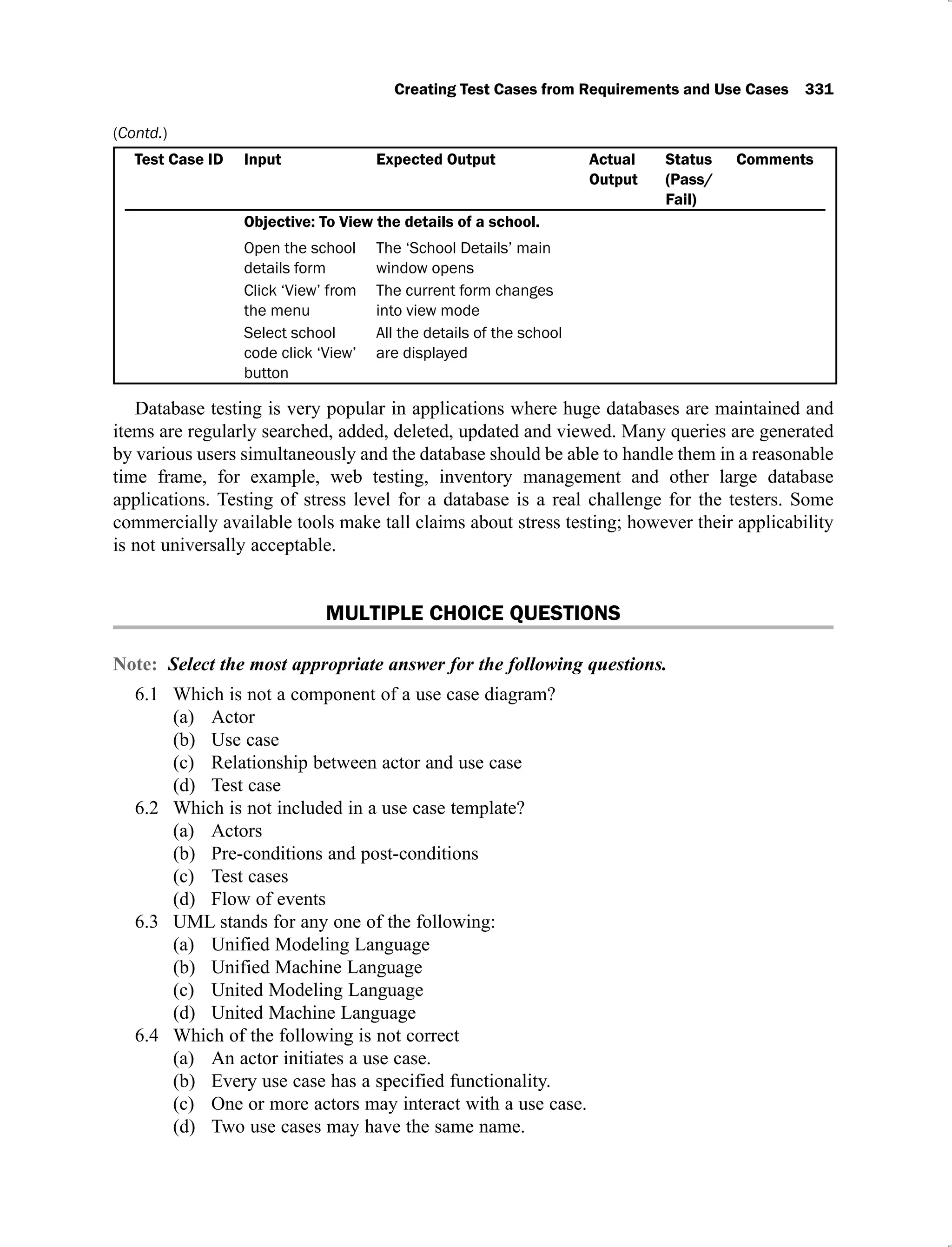
source code is completely ignored.
Test cases are designed on the basis of functionality and internal structure of the
(h)
source code.
Test cases are designed on the basis of pre-conditions and post-conditions.
(i)
Which of the following statement is correct?
2.2
Functional testing is useful in every phase of the software development life cycle.
(a)
Functional testing is more useful than static testing because execution of a program
(b)
gives more confidence.
Reviews are one form of functional testing.
(c)
Structural testing is more useful than functional testing.
(d)
Which of the following is not a form of functional testing?
2.3
Boundary value analysis
(a)
Equivalence class testing
(b)
Data flow testing
(c)
Decision table based testing
(d)
Functional testing is known as:
2.4
Regression Testing
(a)
Load Testing
(b)
Behaviour Testing
(c)
Structural Testing
(d)
For a function of ‘n’ variables, boundary value analysis generates:
2.5
8n + 1 test cases
(a)
6n + 1 test cases
(b)
2n + 1 test cases
(c)
4n + 1 test cases
(d)
For a function of 4 variables, boundary value analysis generates:
2.6
9 test cases
(a)
17 test cases
(b)
33 test cases
(c)
25 test cases
(d)
For a function of ‘n’ variables, robustness testing yields:
2.7
6n + 1 test cases
(a)
8n+ 1 test cases
(b)
2n + 1 test cases
(c)
4n + 1 test cases
(d)
For a function of ‘n’ variables, worst case testing generates:
2.8
6
(a) n
test cases
4
(b) n
+ 1 test cases
Functional Testing 103
5
(c) n
test cases
6
(d) n
+ 1 test cases
For a function of ‘n’ variables, robust worst case testing generates:
2.9
4
(a) n
test cases
6
(b) n
test cases
5
(c) n
test cases
7
(d) n
test cases
A software is designed to calculate taxes to be paid as per details given below:
2.10
Up to Rs. 40,000 : Tax free
(i)
Next Rs. 15,000 : 10% tax
(ii)
Next Rs. 65,000 : 15% tax
(iii)
Above this amount : 20% tax
(iv)
Input to the software is the salary of an employee. Which of the following is a valid
boundary analysis test case?
Rs. 40,000
(a)
Rs. 65,000
(b)
Rs. 1, 20,000
(c)
Rs. 80,000
(d)
‘x’ is an input to a program to calculate the square of the given number. The range for
2.11
‘x’ is from 1 to 100. In boundary value analysis, which are valid inputs?
1,2,50,100,101
(a)
1,2,99,100,101
(b)
1,2,50,99,100
(c)
0,1,2,99,100
(d)
‘x’ is an input to a program to calculate the square of the given number. The range for
2.12
‘x’ is from 1 to 100. In robustness testing, which are valid inputs?
0, 1, 2, 50, 99, 100, 101
(a)
0, 1, 2, 3, 99, 100, 101
(b)
1, 2, 3, 50, 98, 99, 100
(c)
1, 2, 50, 99, 100
(d)
Functionality of a software is tested by:
2.13
White box testing
(a)
Black box testing
(b)
Regression testing
(c)
None of the above
(d)
One weakness of boundary value analysis is:
2.14
It is not effective
(a)
It does not explore combinations of inputs
(b)
It explores combinations of inputs
(c)
None of the above
(d)
Boundary value analysis technique is effective when inputs are:
2.15
Dependent
(a)
Independent
(b)
Boolean
(c)
None of the above
(d)
104 Software Testing
Equivalence class testing is related to:
2.16
Mutation testing
(a)
Data flow testing
(b)
Functional testing
(c)
Structural testing
(d)
In a room air-conditioner, when the temperature reaches 28
2.17 o
C, the cooling is switched
on. When the temperature falls to below 20o
C, the cooling is switched off. What is the
minimum set of test input values (in degree centigrade) to cover all equivalence
classes?
20, 22, 26
(a)
19, 22, 24
(b)
19, 24, 26
(c)
19, 24, 29
(d)
If an input range is from 1 to 100, identify values from invalid equivalence classes.
2.18
0, 101
(a)
10, 101
(b)
0, 10
(c)
None of the above
(d)
In an examination, the minimum passing marks is 50 out of 100 for each subject.
2.19
Identify valid equivalence class values, if a student clears the examination of all three
subjects.
40, 60, 70
(a)
38, 65, 75
(b)
60, 65, 100
(c)
49, 50, 65
(d)
How many minimum test cases should be selected from an equivalence class?
2.20
2
(a)
3
(b)
1
(c)
4
(d)
Decision tables are used in situations where:
2.21
An action is initiated on the basis of a varying set of conditions
(a)
No action is required under a varying set of conditions
(b)
A number of actions are taken under a varying set of conditions
(c)
None of the above
(d)
How many portions are available in a decision table?
2.22
8
(a)
2
(b)
4
(c)
1
(d)
How many minimum test cases are generated by a column of a decision table?
2.23
0
(a)
1
(b)
2
(c)
3
(d)
Functional Testing 105
The decision table which uses only binary conditions is known as:
2.24
Limited entry decision table
(a)
Extended entry decision table
(b)
Advance decision table
(c)
None of the above
(d)
In cause-effect graphing technique, causes and effects are related to:
2.25
Outputs and inputs
(a)
Inputs and outputs
(b)
Sources and destinations
(c)
Destinations and sources
(d)
Cause-effect graphing is one form of:
2.26
Structural testing
(a)
Maintenance testing
(b)
Regression testing
(c)
Functional testing
(d)
Which is not a constraint applicable at the ‘causes’ side in the cause-effect graphing
2.27
technique?
Exclusive
(a)
Inclusive
(b)
Masks
(c)
Requires
(d)
Which is not a basic notation used in a cause-effect graph?
2.28
NOT
(a)
OR
(b)
AND
(c)
NAND
(d)
Which is the term used for functional testing?
2.29
Black box testing
(a)
Behavioural testing
(b)
Functionality testing
(c)
All of the above
(d)
Functional testing does not involve:
2.30
Source code analysis
(a)
Black box testing techniques
(b)
Boundary value analysis
(c)
Robustness testing
(d)
EXERCISES
What is functional testing? How do we perform it in limited time and with limited
2.1
resources?
What are the various types of functional testing techniques? Discuss any one with the
2.2
help of an example.
Explain the boundary value analysis technique with a suitable example.
2.3
106 Software Testing
Why do we undertake robustness testing? What are the additional benefits? Show
2.4
additional test cases with the help of an example and justify the significance of these
test cases.
What is worst-case testing? How is it different from boundary value analysis? List the
2.5
advantages of using this technique.
Explain the usefulness of robust worst-case testing. Should we really opt for this
2.6
technique and select a large number of test cases? Discuss its applicability and
limitations.
Consider a program that determines the previous date. Its inputs are a triple of day,
2.7
month and year with its values in the range:
1 month 12
1 day 31
1850 year 2050
The possible outputs are ‘previous date’ or ‘invalid input’. Design boundary value
analysis test cases, robust test cases, worst-case test cases and robust worst-case test
cases.
Consider the program to find the median of three numbers. Its input is a triple of
2.8
positive integers (say x, y and z) and values are from interval [100,500]. Generate
boundary, robust and worst-case test cases.
Consider a program that takes three numbers as input and print the values of these
2.9
numbers in descending order. Its input is a triple of positive integers (say x, y and z)
and values are from interval [300,700]. Generate boundary value, robust and worst
case test cases.
Consider a three-input program to handle personal loans of a customer. Its input is a
2.10
triple of positive integers (say principal, rate and term).
1000 principal 40000
1 rate 18
1 term 6
The program should calculate the interest for the whole term of the loan and the total
amount of the personal loan. The output is:
interest = principal * (rate/100) * term
total_amount = principal + interest
Generate boundary value, robust and worst-case test cases
The BSE Electrical company charges its domestic consumers using the following
2.11
slab:
Consumption units Energy charges
0–150 2.00 per unit
151–300 Rs 200 + Rs. 3.00 per unit in excess of 150 units
301–400 Rs. 300 + Rs 3.90 per unit in excess of 300 units
>400 Rs. 350 + Rs 4.40 per unit in excess of 400 units
Identify the equivalence class test cases for output and input domain.
An telephone company charges its customer using the following calling rates:
2.12
Functional Testing 107
Call Rates
0-75 Rs. 500
76-200 Rs. 500 + Rs. 0.80 per call in excess of 75 calls
201-500 Rs. 500 + Rs. 1.00 per call in excess of 200 calls
>500 Rs. 500 + Rs 1.20 per unit in excess of 500 calls
Identify the equivalence class test cases for the output and input domain.
Consider an example of grading a student in a university. The grading is done as given
2.13
below:
Average marks Grade
90 – 100 Exemplary Performance
75 – 89 Distinction
60 – 74 First Division
50 – 59 Second Division
0 – 49 Fail
The marks of any three subjects are considered for the calculation of average marks.
Generate boundary value analysis test cases and robust test cases. Also create
equivalence classes and generate test cases.
Consider a program for the classification of a triangle. Its input is a triple of positive
2.14
integers (say, a, b and c) from the interval [1, 100]. The output may be one of the
following words [scalene, Isosceles, Equilateral, Not a triangle]. Design the boundary
value test cases and robust worst-case test cases. Create equivalence classes and design
test cases accordingly.
Consider a program that determines the next date. Given a month, day and year as
2.15
input, it determines the date of the next day. The month, day and year have integer
values subject to the following conditions:
C1
: 1 month 12
C2
: 1 day 31
C3
: 1800 year 2025
We are allowed to add new conditions as per our requirements.
Generate boundary value analysis test cases, robust test cases, worst-case test
(a)
cases and robust worst-case test cases
Create equivalence classes and generate test cases
(b)
Develop a decision table and generate test cases
(c)
Consider a program for the determination of the nature of roots of a quadratic equation.
2.16
Its input is a triple of positive integers (say a, b and c) and values may be from interval
[0, 100]. The output may have one of the following words:
[Not a quadratic equation, Real roots, Imaginary roots, Equal roots]
Design boundary value analysis test cases, robust test cases, worst-case test cases
(a)
and robust worst-case test cases
Create equivalence classes and generate test cases
(b)
Develop a decision table and generate test cases
(c)
Explain the equivalence class testing technique. How is it different from boundary
2.17
value analysis technique?
108 Software Testing
Discuss the significance of decision tables in testing. What is the purpose of a rule
2.18
count? Explain the concept with the help of an example.
What is the cause-effect graphing technique? What are basic notations used in a cause-
2.19
effect graph? Why and how are constraints used in such a graph?
Consider a program to multiply and divide two numbers. The inputs may be two valid
2.20
integers (say a and b) in the range of [0, 100].
Generate boundary value analysis test cases and robust test cases
(a)
Create equivalence class and generate test cases
(b)
Develop a decision table and generate test cases
(c)
Design a cause-effect graph and write test cases accordingly
(d)
Consider the following points based on faculty appraisal and development system of a
2.21
university:
Points Earned University view
1 – 6 Work hard to improve
6 – 8 Satisfactory
8 – 10 Good
10 – 12 Very Good
12 – 15 Outstanding
Generate the test cases using equivalence class testing.
Consider a program to perform binary search and generate the test cases using
2.22
equivalence class testing and decision table based testing.
Write a program to count the number of digits in a number. Its input is any number
2.23
from interval [0, 9999]. Design the boundary value analysis test cases and robustness
test cases.
Why is functional testing also known as black box testing? Discuss with the help of
2.24
examples.
What are the limitations of boundary value analysis technique? Discuss the situations
2.25
in which it is not effective.
FURTHER READING
A resource for pre-1981 literature which contains a huge bibliography up to 1981:
E.F. Miller and W.E. Howden, “Tutorial: Software Testing and Validation
Techniques”, IEEE Computer Society, New York, 1981.
A hands-on guide to the black-box testing techniques:
B. Beizer, “Black-Box Testing: Techniques for Functional Testing of Software
and Systems”, John Wiley and Sons, 1995.
An introductory book on software testing with a special focus on functional testing is:
P. C. Jorgensen, “Software Testing: A Craftsman Approach”, 3rd ed., Auerbach
Publications, New York, 2007.
Other useful texts are:
W.R. Elmendorf, “Cause Effect Graphs in Functional Testing”, TR-00.2487,
IBM System Development Division, Poughkeepsie, New York, 1973.
Functional Testing 109
W.R. Elmendorf, “Functional analysis using cause-effect graphs”, Proceedings
of SHARE XLIII, SHARE, New York, pp. 567–577, 1974.
W.E. Howden, “Functional Program Testing”, IEEE Transactions on Software
Engineering, vol. 6, no. 2, March 1980.
W.E. Howden, “Validation of Scientific Programs”, ACM Computing Surveys
(CSUR), vol.14, no.2, pp.193–227, June 1982.
R.B. Hurley, “Decision Tables in Software Engineering”, Van Nostrand Reinhod,
New York, 1983.
V. Chvalovsky, “Decision tables”, Software Practice and. Experience, vol. 13,
pp. 423–429, 1983.
B. Korel and J. Laski, “A Tool for Data Flow Oriented Program Testing”, Second
Conference on Software Development Tools, Techniques, and Alternatives, San
Francisco, CA, December 25, 1985.
V.R. Basili and R.W. Selby, “Comparing the Effectiveness of Software Testing
Strategies”, vol. 13, pp. 1278–1296, 1987.
3
Essentials of Graph Theory
Graphtheoryhasbeenusedextensivelyincomputerscience,electricalengineering,communication
systems, operational research, economics, physics and many other areas. Any physical situation
involving discrete objects may be represented by a graph along with their relationships amongst
them. In practice, there are numerous applications of graphs in modern science and technology.
Graph theory has recently been used for representing the connectivity of the World Wide Web.
Global internet connectivity issues are studied using graphs like the number of links required to
move from one web page to another and the links which are used to establish this connectivity.
It has also provided many ways to test a program. Some testing techniques are available which
are based on the concepts of graph theory.
3.1 WHAT IS A GRAPH?
A graph has a set of nodes and a set of edges that connect these nodes. A graph G = (V, E)
consists of a non-empty finite set V of nodes and a set E of edges containing ordered or
unordered pairs of nodes.
V = (n1
, n2
, n3
……..nm
) and E = (e1
, e2
, e3
………ek
)
If an edge ei
E is associated with an ordered pair <ni
, nj
> or an unordered pair (ni
, nj
),
where ni
, nj
V, then the ei
is said to connect the nodes ni
and nj
. The edge ei
that connects the
node ni
and nj
is called incident on each of the nodes. The pair of nodes that are connected by
an edge are called adjacent nodes. A node, which is not connected to any other node, is called
an isolated node. A graph with only isolated nodes is known as null graph.
If in graph G = (V, E), each edge ei
E is associated with an ordered pair of nodes, then
graph G is called a directed graph or digraph. If each edge is associated with an unordered pair
of nodes, then a graph G is called an undirected graph.
In diagrammatical representation of a graph, nodes are represented by circles and edges are
represented by lines joining the two nodes incident on it and the same is shown in Figure 3.1.
Essentials of Graph Theory 111
Figure 3.1. Undirected and directed graphs
In the Figure 3.1(a), the node and edge sets are given as:
V = (n1
, n2
, n3
, n4
, n5
, n6
)
E = (e1
, e2
, e3
, e4
) = ((n1
, n2
), (n1
, n3
), (n2
, n4
), (n2
, n5
))
Similarly in Figure 3.1(b), the node and edge sets are
V= (n1
, n2
, n3
, n4
, n5
, n6
)
E = (e1
, e2
, e3
, e4
) = (<n1
, n2
>, <n1
, n3
>, <n2
, n4
>, <n2
, n5
>)
The only difference is that edges are the ordered pairs of nodes represented by <n1
, n2
>
rather than unordered pairs (n1
, n2
). For any graph (directed or undirected), a set of nodes and
a set of edges between pairs of nodes are required for the construction of the graph.
An edge of a graph having the same node at its end points is called a loop. The direction of
the edge is not important because the initial and final nodes are one and the same. In Figure
3.2(a), edge e1
is a loop with node n1
and may be represented as e1
= (n1
, n1
).
Figure 3.2. Undirected graphs with loop and parallel edges
112 Software Testing
If certain pairs of nodes are connected by more than one edge in a directed or undirected
graph, then these edges are known as parallel edges. In Figure 3.2(b), e1
and e2
are parallel
edges connecting nodes n1
and n2
. Similarly e5
and e6
are also parallel edges connecting nodes
n2
and n5
. If a graph is a directed graph and parallel edges are in opposite directions, such edges
are considered as distinct edges. A graph that has neither loops nor parallel edges is called a
simple graph. A graph with one or more parallel edges is called a multigraph. These graphs are
shown in Figure 3.3.
Figure 3.3. Types of graphs
A directed multigraph (see Figure 3.3 (c)) may have distinct parallel edges (like e1
and e2
)
and parallel edges (like e5
and e6
). If numbers or weights are assigned to each edge of a graph,
then such a graph is called a weighted graph.
3.1.1 Degree of a Node
The degree of a node in an undirected graph is the number of edges incident on it. However, a
loop contributes twice to the degree of that node. The degree of a node ‘n’ is represented by
deg(n). The degrees of nodes in a graph shown in Figure 3.1 (a) are given as:
deg(n1
) = 2, deg(n2
) = 3, deg(n3
) = 1, deg(n4
) = 1, deg(n5
) = 1, deg(n6
) = 0
The degree of an isolated node is always 0. In case of directed graphs, the direction of edges
play an important role and indegree and outdegree of a node is calculated. Indegree of a node
in a directed graph is the number of edges that are using that node as a terminal node. The
indegree of a node ‘n’ is represented by indeg(n). The outdegree of a node in a directed graph
is the number of edges that are using that node as a start node. The outdegree of a node ‘n’ is
represented by outdeg(n). The indegrees and outdegrees of nodes in a graph shown in Figure
3.1(b) are given as:
indeg(n1
) = 0 outdeg(n1
) = 2
indeg(n2
) = 1 outdeg(n2
) = 2
indeg(n3
) = 1 outdeg(n3
) = 0
Essentials of Graph Theory 113
indeg(n4
) = 1 outdeg(n4
) = 0
indeg(n5
) = 1 outdeg(n5
) = 0
indeg(n6
) = 0 outdeg(n6
) = 0
The degree of a node in a directed graph is the sum of indegree and outdegree of that node.
Hence, for node ‘n’ in a directed graph, the degree is given as:
deg(n) = indeg(n) + outdeg(n)
Few important characteristics of nodes are identified on the basis of indegree and outdegree
and are given as:
Source node: A node with indegree = 0 and outdegree
(i) 1
Destination node: A node with outdegree = 0 and in degree
(ii) 1
Sequential node: A node with indegree = 1 and outdegree = 1
(iii)
Predicate/decision node: A node with outdegree
(iv) 2
Junction node: indegree
(v) 2
In Figure 3.1(b), source nodes: n1
Destination nodes: n3
, n4
, n5
Sequential nodes: nil
Predicate nodes: n1
, n2
There is no junction node in this graph and n6
is an isolated node.
3.1.2 Regular Graph
If every node of a simple graph has the same degree, then the graph is called a regular graph.
If the degree of a node is ‘n’, then it is called n-regular graph. Some of such graphs are shown
in Figure 3.4.
Figure 3.4. Regular graphs
3.2 MATRIX REPRESENTATION OF GRAPHS
In computer science, matrix representation of graphs is very popular due to its direct applications
in programming. Each piece of information of a graph, which is shown diagrammatically, can be
114 Software Testing
converted into matrix form. Some useful matrix representations are given in the following sub-
sections which are used commonly in testing.
3.2.1 Incidence Matrix
Consider a graph G = (V, E) where
V = (n1
, n2
, n3
…..nm
)
E = (e1
, e2
, e3
……ek
)
In this graph, there are ‘m’ nodes and ‘k’ edges. An incidence matrix is a matrix with ‘m’
rows and ‘k’ columns whose elements are defined such that:
a(i, j)
1 if j edge e is incident on i node n
0 other
th
j
th
i
w
wise
The incidence matrix of a graph shown in Figure 3.1(a) is given as:
n
n
n
n
n
n
1 0 0
0 1 1
1
3
4
5
6
2
1
1
0 1 0 0
0 1 0
0 0 1
0
0
0
0 0 0
e e e e
2 3 4
1
The sum of entries of any column of incidence matrix is always 2. This is because a column
represents an edge which has only two endpoints. If, any time, the sum is not two, then there
is some mistake in the transfer of information. If we add entries of a row, which is corresponding
to a node, we get the degree of that node. If all entries of a row are 0’s, then the corresponding
node is an isolated node. Incidence matrix of a graph may be used to calculate various
properties of a graph which can further be programmed, if so desired. The incidence matrix of
a directed graph is the same as the incidence matrix of an undirected graph.
3.2.2 Adjacency Matrix
It is also known as connection matrix because it represents connections in a graph. The
adjacency matrix of a graph G = (V, E) with ‘m’ nodes is a square matrix of size m×m whose
elements are defined such that:
a(i, j)
1 if there is an edge from nodes n and n
0 other
i j
w
wise
The adjacency matrix of a graph shown in Figure 3.1(a) is given as:
Essentials of Graph Theory 115
n n n n n n
n
n
n
n
n
n
0 1
1 2 3 4 5 6
1
3
4
5
6
2
1 0 0 0
1 0 0 1 1 0
0
0 0 0
0 1 0 0 0 0
1 0 0 0 0
0 0 0 0 0 0
1 0 0
0
If we add entries of any row, we get the degree of the node corresponding to that row. This
is similar to incidence matrix. The adjacency matrix of an undirected graph is symmetric where
a(i, j) = a(j, i).
If we represent connections with the name of edges, then the matrix is called graph matrix.
The size is the same as adjacent matrix i.e. number of nodes in a graph. The graph matrix of a
graph shown in Figure 3.1(a) is given as:
n n n n n n
n
n
n
n
n
n
0 e e
1 2 3 4 5 6
1
3
4
5
6
1
2
2
2
1 3 4
0 0 0
0 0 0
0 0 0
0 0 0 0 0
0 0 0 0
0 0 0 0 0 0
e e e
e 0 0
e
0 e
2
3
4
If connections are represented by 1, then it becomes the connection matrix.
The adjacency matrix of a directed graph G = (V, E) with ‘m’ nodes is a square matrix of
size m×m whose elements are such that:
a(i, j)
1 if there is an edge from nodes n and n
0 other
i j
w
wise
The adjacency matrix of a directed graph may not be symmetric. If we add entries of a row,
it becomes outdegree of the node and if we add entries of a column, it becomes indegree of the
node. The adjacency matrix of a directed graph given in Figure 3.1(b) is given as:
n n n n n n
n
n
n
n
n
n
0 1
1 2 3 4 5 6
1
3
4
5
6
2
1 0 0 0
0 0 0 1 1 0
0
0 0 0
0 0 0 0 0 0
0 0 0 0 0
0 0 0 0 0 0
0 0 0
0
116 Software Testing
In directed graph, direction of an edge is considered, hence adjacency matrix of a directed
graph is different from the undirected graph.
3.3 PATHS AND INDEPENDENT PATHS
A path in a graph is a sequence of adjacent nodes where nodes in sequence share a common
edge or sequence of adjacent pair of edges where edges in sequence share a common node. The
paths in a graph shown in Figure 3.1(a) are given in Table 3.1.
Table 3.1. Paths of undirected graph in Figure 3.1(a)
S.No. Paths from initial node to Sequence of nodes Sequence of edges
1. n1
to n4
n1
,n2
,n4
e1
,e3
2. n1
to n5
n1
,n2
,n5
e1
,e4
3. n1
to n2
n1
,n2
e1
4. n1
to n3
n1
,n3
e2
5. n2
to n4
n2
,n4
e3
6. n2
to n5
n2
,n5
e4
7. n2
to n1
n2
,n1
e1
8. n3
to n1
n3
,n1
e2
9. n4
to n2
n4
,n2
e3
10. n4
to n1
n4
,n2
,n1
e3
,e1
11. n5
to n2
n5
,n2
e4
12. n5
to n1
n5
,n2
,n1
e4
,e1
13. n2
to n3
n2
,n1
, n3
e1
,e2
14. n3
to n2
n3
,n1
, n2
e2
,e1
15. n4
to n3
n4
,n2
, n1
, n3
e3
,e1
, e2
16. n3
to n4
n3
,n1
, n2
, n4
e2
,e1
, e3
17. n4
to n5
n4
,n2
, n5
e3
,e4
18. n5
to n4
n5
,n2
, n4
e4
,e3
19. n5
to n3
n5
,n2
, n1
, n3
e4
,e1
, e2
20. n3
to n5
n3
,n1
, n2
, n5
e2
,e1
, e4
A path represented by sequence of nodes is a more popular representation technique than
sequence of edges.
An independent path in a graph is a path that has at least one new node or edge in its
sequence from the initial node to its final node.
If there is no repetition of an edge in a path from the initial node to the final node, then the
path is called a simple path. The number of edges in a path is called the length of the path.
Essentials of Graph Theory 117
The direction of an edge provides more meaning to a path. Hence, paths of a directed graph
seem to be more practical and useful. They are also called chains. The paths in a directed graph
shown in Figure 3.1(b) are given in Table 3.2.
Table 3.2. Paths of directed graph in Figure 3.1(b)
S.No.
Paths from initial node to
Sequence of nodes Sequence of edges
1. n1
to n4
n1
,n2
,n4
e1
,e3
2. n1
to n5
n1
,n2
,n5
e1
,e4
3. n1
to n2
n1
,n2
e1
4. n1
to n3
n1
,n3
e2
5. n2
to n4
n2
,n4
e3
6. n2
to n5
n2
,n5
e4
3.3.1 Cycles
When the initial and final nodes of a path are the same and if length 0, the path is called a
cycle. Consider the graph given in Figure 3.5 having 6 nodes and 6 edges with a cycle
constituted by a path n1
, n2
, n5
, n3
, n1
of length 4.
Figure 3.5. Cyclic graph
3.3.2 Connectedness of a Graph
An undirected graph is said to be connected if there is a path between every pair of nodes of
the graph, otherwise it is said to be a disconnected graph. Two nodes are also said to be
connected if there is a path between them.
A graph shown in Figure 3.3 (a) is a connected graph and a graph shown in Figure 3.1 (a)
is a disconnected graph. The graph shown in Figure 3.6 is a disconnected graph with two
portions of the graph.
118 Software Testing
Figure 3.6. Disconnected graphs
A disconnected graph is the union of two or more disjoint portions of the graph. These
disjoint portions are called the connected components of the graph.
A directed graph is said to be strongly connected if there is a path from node ni
to node nj
;
where node ni
and nj
are any pair of nodes of the graph.
Every node of the graph should have a path to every other node of the graph in the strongly
connected graphs. The directed graph shown in Figure 3.7 is a strongly connected graph.
Figure 3.7. Strongly connected graph
The graph shown in Figure 3.7 has the following pair of nodes:
<n1
, n2
>, <n1
, n3
>, <n4
, n1
>, <n3
, n2
>, <n2
, n4
>, <n3
, n4
>. We identify paths for every pair of
nodes.
Pair <n
(a) 1
, n2
>: Path = n1
, n2
Pair <n2
, n1
>: Path = n2
, n4
,n1
Essentials of Graph Theory 119
Pair <n
(b) 1
, n3
>: Path = n1
, n3
Pair <n3
, n1
>: Path = n3
, n4
, n1
Pair <n
(c) 1
, n4
>: Path = n1
, n2
, n4
Pair <n4
, n1
>: Path = n4
, n1
Pair <n
(d) 2
, n3
>: Path = n2
, n4
, n1
,n3
Pair <n3
, n2
>: Path = n3
, n2
Pair <n
(e) 2
, n4
>: Path = n2
, n4
Pair <n4
, n2
>: Path = n4
, n1
, n2
Pair <n
(f) 3
, n4
>: Path = n3
, n4
Pair <n4
, n3
>: Path = n4
, n1
, n3
Hence this graph is strongly connected.
A directed graph is said to be weakly connected, if there is a path between every two nodes
when the directions of the edges are not considered. A strongly connected directed graph will
also be weakly connected when we do not consider the directions of edges. Consider the graph
shown in Figure 3.8 which is weakly connected.
Figure 3.8. Weakly connected graph
When we do not consider the directions, it becomes an undirected graph where there is a
path between every two nodes of the graph. Hence, this graph is weakly connected but not
strongly connected.
Example 3.1: Consider the following undirected graph and find:
The degree of all nodes
(a)
The incidence matrix
(b)
Adjacency matrix
(c)
Paths
(d)
120 Software Testing
Solution:
This graph is an undirected graph with seven nodes and six edges
The degrees of nodes are given as:
(a)
deg(n1
) = 2 deg(n5
) = 1
deg(n2
) = 3 deg(n6
) = 1
deg(n3
) = 3 deg(n7
) = 1
deg(n4
) = 1
Incidence matrix of this graph has 7 × 6 size which is given as:
(b)
e e e e e e
n
n
n
n
n
n
n
1 1 0 0 0 0
1 0 1
1 2 3 4 5 6
1
2
3
4
5
6
7
1
1 0 0
0 1 0 0 1 1
0 0 1 0 0 0
0 0 0 1 0 0
0 0 0 0 1 0
0 0 0 0 0 1
Adjacency matrix with size 7 × 7 is given as:
(c)
n n n n n n n
n
n
n
n
n
n
n
1 2 3 4 5 6 7
1
2
3
4
5
6
7
0 1 1 0 0 0 0
1 0 0 1 1 0 0
1 0
0 0 0 0 1 1
0 1 0 0 0 0 0
0 1 0 0 0 0 0
0 0 1 0 0 0 0
0 0 1 0 0 0 0
Paths of the graph are given as:
(d)
Essentials of Graph Theory 121
S. No. Paths from initial node to Sequence of nodes Sequence of edges
1. n1
to n2
n1
,n2
e1
2. n1
to n4
n1
,n2
,n4
e1
,e3
3. n1
to n5
n1
,n2
,n5
e1
,e4
4. n1
to n3
n1
,n3
e2
5. n1
to n6
n1
,n3
,n6
e2
,e5
6. n1
to n7
n1
,n3
,n7
e2
,e6
7. n2
to n1
n2
,n1
e1
8. n2
to n4
n2
,n4
e3
9. n2
to n5
n2
,n5
e4
10. n3
to n1
n3
,n1
e2
11. n3
to n6
n3
, n6
e5
12. n3
to n7
n3
, n7
e6
13. n4
to n2
n4
,n2
e3
14. n4
to n1
n4
,n2
,n1
e3
,e1
15. n5
to n2
n5
,n2
e4
16. n5
to n1
n5
,n2
,n1
e4
,e1
17. n6
to n3
n6
,n2
e5
18. n6
to n1
n6
,n3
,n1
e5
,e2
19. n7
to n3
n7
,n3
e6
20. n7
to n1
n7
,n3
,n1
e6
,e2
21. n2
to n3
n2
,n1
, n3
e1
,e2
22. n2
to n6
n2
,n1
, n3
, n6
e1
,e2
, e5
23. n2
to n7
n2
,n1
, n3
, n7
e1
,e2
, e6
24. n3
to n2
n3
,n1
, n2
e2
,e1
25. n3
to n4
n3
,n1
, n2
, n4
e2
,e1
, e3
26. n3
to n5
n3
,n1
, n2
, n5
e1
,e2
, e4
27. n4
to n3
n4
,n2
, n1
, n3
e3
,e1
, e2
28. n4
to n5
n4
,n2
, n5
e3
,e4
29. n4
to n6
n4
,n2
, n1
, n3
, n6
e3
,e1
, e2
, e5
30. n4
to n7
n4
,n2
, n1
, n3
, n7
e3
,e1
, e2
, e6
31. n5
to n3
n5
,n2
, n1
, n3
e4
,e1
, e2
32. n5
to n4
n5
,n2
, n4
e4
,e3
33. n5
to n6
n5
,n2
, n1
, n3
, n6
e4
,e1
, e2
, e5
34. n5
to n7
n5
,n2
, n1
, n3
, n7
e4
,e1
, e2
, e6
35. n6
to n2
n6
, n3
,n1
, n2
e5
,e2
, e1
36. n6
to n4
n6
,n3
, n1
, n2
, n4
e5
,e2
, e1
, e3
37. n6
to n5
n6
,n3
, n1
, n2
, n5
e5
,e2
, e1
, e4
38. n6
to n7
n6
,n3
, n7
e5
,e6
39. n7
to n2
n7
, n3
,n1
, n2
e6
,e2
, e1
40. n7
to n4
n7
,n3
, n1
, n2
, n4
e6
,e2
, e1
, e3
41. n7
to n5
n7
,n3
, n1
, n2
, n5
e6
,e2
, e1
, e4
42. n7
to n6
n7
,n3
, n6
e6
,e5
122 Software Testing
Example 3.2: Consider the following directed graph and find:
The degree of all nodes
(a)
The incidence matrix
(b)
Adjacency matrix
(c)
Paths
(d)
Connectedness
(e)
Solution:
This graph is a directed graph with seven nodes and six edges
The degrees of all nodes are given as:
(a)
indeg(n1
) = 0 outdeg(n1
) = 2 deg(n1
) = 2
indeg(n2
) = 1 outdeg(n2
) = 2 deg(n2
) = 3
indeg(n3
) = 1 outdeg(n3
) = 2 deg(n3
) = 3
indeg(n4
) = 1 outdeg(n4
) = 0 deg(n4
) = 1
indeg(n5
) = 1 outdeg(n5
) = 0 deg(n5
) = 1
indeg(n6
) = 1 outdeg(n6
) = 0 deg(n6
) = 1
indeg(n7
) = 1 outdeg(n7
) = 0 deg(n7
) = 1
Incidence matrix of this graph has 7 × 6 is given as:
(b)
e e e e e e
n
n
n
n
n
n
n
1 1 0 0 0 0
1 0 1
1 2 3 4 5 6
1
2
3
4
5
6
7
1
1 0 0
0 1 0 0 1 1
0 0 1 0 0 0
0 0 0 1 0 0
0 0 0 0 1 0
0 0 0 0 0 1
Adjacency matrix with size 7 × 7 is given as:
(c)
Essentials of Graph Theory 123
n n n n n n n
n
n
n
n
n
n
n
1 2 3 4 5 6 7
1
2
3
4
5
6
7
0 1 1 0 0 0 0
1 0 0 1 1 0 0
0 0
0 0 0 0 1 1
0 0 0 0 0 0 0
0 0 0 0 0 0 0
0 0 0 0 0 0 0
0 0 0 0 0 0 0
Paths of the graph are given as:
(d)
S. No. Paths from initial node to Sequence of nodes Sequence of edges
1. n1
to n2
n1
,n2
e1
2. n1
to n4
n1
,n2
,n4
e1
,e3
3. n1
to n5
n1
,n2
,n5
e1
,e4
4. n1
to n3
n1
,n3
e2
5. n1
to n6
n1
,n3
,n6
e2
,e5
6. n1
to n7
n1
,n3
,n7
e2
,e6
7. n2
to n4
n2
,n4
e3
.8. n2
to n5
n2
,n5
e4
9. n3
to n6
n3
, n6
e5
10. n3
to n7
n3
, n7
e6
This graph is weakly connected because there is no path between several nodes; for
(e)
example, from node n4
to n2
, n6
to n3
, n3
to n1
, n2
to n1
, etc. however, if we do not
consider directions, there is a path from every node to every other node which is the
definition of a weakly connected graph.
3.4 GENERATION OF A GRAPH FROM PROGRAM
Graphs are extensively used in testing of computer programs. We may represent the flow of
data and flow of control of any program in terms of directed graphs. A graph representing the
flow of control of a program is called a program graph. The program graph may further be
transformed into the DD path graph. Both of these graphs may provide foundations to many
testing techniques.
124 Software Testing
3.4.1 Program Graphs
Program graph is a graphical representation of the source code of a program. The statements
of a program are represented by nodes and flow of control by edges in the program graph. The
definition of a program graph is [JORG07]:
“A program graph is a directed graph in which nodes are either statements or fragments
of a statement and edges represent flow of control.”
The program graph helps us to understand the internal structure of the program which may
provide the basis for designing the testing techniques. The basic constructs of the program
graph are given in Figure 3.9.
Figure 3.9. Basic constructs of a program graph
The basic constructs are used to convert a program in its program graph. We consider the
program ‘Square’ which takes a number as an input and generates the square of the number.
This program has 8 sequential statements which are represented by 8 nodes. All nodes are
arranged sequentially which may lead to only one path in this program graph. Every program
graph has one source node and one destination node.
Essentials of Graph Theory 125
We also consider a program given in Figure 3.11 that takes three numbers as input and prints
the largest amongst these three numbers as output. The program graph of the program is given
in Figure 3.12. There are 28 statements in the program which are represented by 28 nodes. All
nodes are not in a sequence which may lead to many paths in the program graph.
1 2 3 4 6 7 8
5
(b) Program graph for 'Square' program
#include<stdio.h>
1 void main()
2 {
3 int num, result;
4 printf(“Enter the number:”);
5 scanf(“%d”, &num);
6 result=num*num;
7 printf(“The result is: %d”, result);
8 }
(a) Program to find 'square' of a number
Figure 3.10. Program ‘Square’ and its program graph
#include<stdio.h>
#include<conio.h>
1. void main()
2. {
3. float A,B,C;
4. clrscr();
5. printf("Enter number 1:n");
6. scanf("%f", &A);
7. printf("Enter number 2:n");
8. scanf("%f", &B);
9. printf("Enter number 3:n");
10. scanf("%f", &C);
/*Check for greatest of three numbers*/
11. if(A>B) {
12. if(A>C) {
13. printf("The largest number is: %fn",A);
14. }
15. else {
16. printf("The largest number is: %fn",C);
17. }
18. }
19. else {
20. if(C>B) {
21. printf("The largest number is: %fn",C);
22. }
(Contd.)
126 Software Testing
23. else {
24. printf("The largest number is: %fn",B);
25. }
26. }
27. getch();
28. }
Figure 3.11. Program to find the largest among three numbers
Figure 3.12. Program graph to find the largest number amongst three numbers as given in Figure 3.11.
Our example is simple, so it is easy to find all paths starting from the source node (node 1)
and ending at the destination node (node 28). There are four possible paths. Every program
graph may provide some interesting observations about the structure of the program. In our
program graph given in Figure 3.12, nodes 2 to 10 are in sequence and nodes 11, 12, and 20
have two outgoing edges (predicate nodes) and nodes 18, 26, 27 have two incoming edges are
(junction nodes).
We may also come to know whether the program is structured or not. A large program may
be a structured program whereas a small program may be unstructured due to a loop in a
program. If we have a loop in a program, large number of paths may be generated as shown in
figure 1.5 of chapter 1. Myers [MYER04] has shown 1014
paths in a very small program graph
due to a loop that iterates up to 20 times. This shows how an unstructured program may lead
to difficulties in even finding every possible path in a program graph. Hence, testing a
structured program is much easier as compared to any unstructured program.
(Contd.)
Essentials of Graph Theory 127
3.4.2 DD Path Graphs
The Decision to Decision (DD) path graph is an extension of a program graph. It is widely
known as DD path graph. There may be many nodes in a program graph which are in a
sequence. When we enter into the first node of the sequence, we can exit only from the last
node of that sequence. In DD path graph, such nodes which are in a sequence are combined
into a block and are represented by a single node. Hence, the DD path graph is a directed graph
in which nodes are sequences of statements and edges are control flow amongst the nodes. All
programs have an entry and an exit and the corresponding program graph has a source node
and a destination node. Similarly, the DD path graph also has a source node and a destination
node.
We prepare a mapping table for the program graph and the DD path graph nodes. A mapping
table maps nodes of the program graph to the corresponding nodes of the DD path graph. This
may combine sequential nodes of the program graph into a block and that is represented by a
single node in the DD path graph. This process may reduce the size of the program graph and
convert it into a more meaningful DD path graph. We consider program ‘Square’ and its
program graph given in Figure 3.10. We prepare a mapping table and a DD path graph as
shown in Figure 3.13. All nodes are sequential nodes except node 1 and node 8 which are
source node and destination node respectively.
Program graph
nodes
DD path graph
corresponding
nodes
Remarks
1 S Source node
2 – 7 N1
8 D Destination node
Figure 3.13. DD path graph and mapping table of program graph in Figure 3.10
We consider a program to find the ‘largest amongst three numbers’ as given in Figure 3.11.
The program graph is also given in Figure 3.12. There are many sequential nodes, decision
nodes, junction nodes available in its program graph. Its mapping table and the DD path graph
are given in Table 3.3 and Figure 3.14 respectively.
Table 3.3. Mapping of program graph nodes and DD graph nodes
Program graph nodes DD path graph
corresponding node
Remarks
1 S Source node
2 to 10 N1
node 2 to 10
11 N2 Decision node, if true goto 12, else goto 19
12 N3 Decision node, if true goto 13 else goto 15
13, 14 N4 Sequential nodes
15, 16, 17 N5 Sequential nodes
Mapping of program graph nodes and DD path graph nodes
(Contd.)
128 Software Testing
Program graph nodes DD path graph
corresponding node
Remarks
18 N6 Junction node, two edges 14 and 17 are termi-
nated here
19 N7 Intermediate node terminated at node 20
20 N8 Decision node, if true goto 21 else goto 23
21, 22 N9 Sequential nodes
23, 24, 25 N10 Sequential nodes
26 N11 Junction node, two edges 22 and 25 are termi-
nated here
27 N12 Junction node, two edges 18 and 26 are termi-
nated here
28 D Destination node
Figure 3.14. DD path graph of the program to find the largest among three numbers.
(Contd.)
Essentials of Graph Theory 129
The DD path graphs are used to find paths of a program. We may like to test every identified
path during testing which may give us some level of confidence about the correctness of the
program.
Example 3.3: Consider the program for the determination of division of a student. Its input is
a triple of positive integers (mark1, mark2, mark3) and values are from interval [0, 100].
The program is given in Figure 3.15. The output may be one of the following words:
[First division with distinction, First division, Second division, Third division, Fail, Invalid
marks]. Draw the program graph and the DD path graph.
Solution:
The program graph is given in Figure 3.16. The mapping table of the DD path graph is given
in Table 3.4 and DD path graph is given in Figure 3.17.
/*Program to output division of a student based on the marks in three subjects*/
#include<stdio.h>
#include<conio.h>
1. void main()
2. {
3. int mark1, mark2,mark3,avg;
4. clrscr();
5. printf("Enter marks of 3 subjects (between 0-100)n");
6. printf("Enter marks of first subject:");
7. scanf("%d", &mark1);
8. printf("Enter marks of second subject:");
9. scanf("%d", &mark2);
10. printf("Enter marks of third subject:");
11. scanf("%d",&mark3);
12. if(mark1>100||mark1<0||mark2>100||mark2<0||mark3>100||mark3<0) {
13. printf("Invalid Marks! Please try again");
14. }
15. else {
16. avg=(mark1+mark2+mark3)/3;
17. if(avg<40) {
18. printf("Fail");
19. }
20. else if(avg>=40&&avg<50) {
21. printf("Third Division");
22. }
23. else if(avg>=50&&avg<60) {
24. printf("Second Division");
25. }
(Contd.)
130 Software Testing
26. else if(avg>=60&&avg<75) {
27. printf("First Division");
28. }
29. else {
30. printf("First Division with Distinction");
31. }
32. }
33. getch();
34. }
Figure 3.15. Source code of determination of division of a student problem
Figure 3.16. Program graph
(Contd.)
Essentials of Graph Theory 131
Table 3.4. Mapping of program graph nodes and DD graph nodes
Program graph
nodes
DD path graph
corresponding node
Remarks
1 S Source node
2 to 11 N1 Sequential nodes, there is a sequential
12 N2 Decision node, if true goto 13 else goto
15
13, 14 N3 Sequential nodes
15, 16 N4 Sequential nodes
17 N5 Decision node, if true goto 18 else goto
20
18, 19 N6 Sequential nodes
20 N7 Decision node, if true goto 21 else goto
23
21, 22 N8 Sequential nodes
23 N9 Decision node, if true goto 24 else goto
26
24, 25 N10 Sequential nodes
26 N11 Decision node, if true goto 27 else goto
29
27, 28 N12 Sequential nodes
29, 31 N13 Sequential nodes
32 N14
and 31 are terminated here
33 N15 Junction node, two edges 14 and 32 are
terminated here
34 D Destination node
Example 3.4: Consider the program for classification of a triangle. Its input is a triple of
positive integers (say a, b and c) and values from the interval [1, 100]. The output may be
[Right angled triangle, Acute angled triangle, Obtuse angled triangle, Invalid triangle, Input
values are out of Range]. The program is given in Figure 3.18. Draw the program graph and
the DD path graph.
Solution:
The program graph is shown in Figure 3.19. The mapping table is given in Table 3.5 and the
DD path graph is given in Figure 3.20.
132 Software Testing
Figure 3.17. DD path graph of program to find division of a student
/*Program to classify whether a triangle is acute, obtuse or right angled given the sides of
the triangle*/
//Header Files
#include<stdio.h>
#include<conio.h>
#include<math.h>
1. void main() //Main Begins
2. {
(Contd.)
Essentials of Graph Theory 133
3. double a,b,c;
4. double a1,a2,a3;
5. int valid=0;
6. clrscr();
7. printf("Enter first side of the triangle:"); /*Enter the sides of Triangle*/
8. scanf("%lf",&a);
9. printf("Enter second side of the triangle:");
10. scanf("%lf",&b);
11. printf("Enter third side of the triangle:");
12. scanf("%lf",&c);
/*Checks whether a triangle is valid or not*/
13. if(a>0&&a<=100&&b>0&&b<=100&&c>0&&c<=100) {
14. if((a+b)>c&&(b+c)>a&&(c+a)>b) {
15. valid=1;
16. }
17. else {
18. valid=-1;
19. }
20. }
21. if(valid==1) {
22. a1=(a*a+b*b)/(c*c);
23. a2=(b*b+c*c)/(a*a);
24. a3=(c*c+a*a)/(b*b);
25. if(a1<1||a2<1||a3<1) {
26. printf("Obtuse angled triangle");
27. }
28. else if(a1==1||a2==1||a3==1) {
29. printf("Right angled triangle");
30. }
31. else {
32. printf("Acute angled triangle");
33. }
34. }
35. else if(valid==-1) {
36. printf("nInvalid Triangle");
37. }
38. else {
39. printf("nInput Values are Out of Range");
(Contd.)
(Contd.)
134 Software Testing
40. }
41. getch();
42. } //Main Ends
Figure: 3.18. Source code for classification of triangle problem
Figure 3.19. Program graph of classification of triangle problem
(Contd.)
Essentials of Graph Theory 135
Table 3.5. Mapping of program graph nodes and DD graph nodes
Program graph nodes DD path graph
corresponding node
Remarks
1 S Source node
2 to 12 N1 Sequential nodes, there is a sequential
13 N2 Decision node, if true goto 14 else goto
21
14 N3 Decision node, if true goto 15 else goto
17
15, 16 N4 Sequential nodes
17, 18, 19 N5 Sequential nodes
20 N6 Junction node, two edges 16 and 19
are terminated here
21 N7 Junction node, two edges 13 and 20
are terminated here. Also a decision
node, if true goto 22, else goto 35
22, 23, 24 N8 Sequential nodes
25 N9 Decision node, if true goto 26 else goto
28
26, 27 N10 Sequential nodes
28 N11 Decision node, if true goto 29 else goto
31
29, 30 N12 Sequential nodes
31, 32, 33 N13 Sequential nodes
34 N14 Junction node, three edges 27, 30 and
33 are terminated here
35 N15 Decision node, if true goto 36 else goto
38
36, 37 N16 Sequential nodes
38, 39, 40 N17 Sequential nodes
41 N18 Three edges 34, 37 and 40 are termi-
nated here.
42 D Destination node.
136 Software Testing
Figure 3.20. DD path graph of the program to classify a triangle
Example 3.5: Consider the program for determining the day of the week. Its input is a triple
of day, month and year with the values in the range
1 month 12
1 day 31
1900 year 2058
The possible values of the output may be [Sunday, Monday, Tuesday, Wednesday, Thursday,
Friday, Saturday, Invalid date]. The program is given in Figure 3.21.
Essentials of Graph Theory 137
Draw the program graph and the DD path graph.
/*Program to compute day of the week*/
/*Header Files*/
#include<stdio.h>
#include<conio.h>
1. void main()
2. {
3. int day,month,year,century,Y,y1,M,date,validDate=0,leap=0;
4. clrscr();
5. printf("Enter day:");
6. scanf("%d",&day);
7. printf("Enter month:");
8. scanf("%d",&month);
9. printf("Enter year (between 1900 and 2058):");
10. scanf("%d",&year);
/*Check whether the date is valid or not*/
11. if(year>=1900&&year<=2058) {
12. if(year%4==0) { /*Check for leap year*/
13. leap=1;
14. if((year%100)==0&&(year%400)!=0) {
15. leap=0;
16. }
17. }
18. if(month==4||month==6||month==9||month==11){
19. if(day>=1&&day<=30) {
20. validDate=1;
21. }
22. else {
23. validDate=0;
24. }
25. }
26. else if(month==2){
27. if(leap==1&&(day>=1&&day<=29)) {
28. validDate=1;
29. }
30. else if(day>=1&&day<=28) {
31. validDate=1;
32. }
33. else {
34. validDate=0;
35. }
36. }
37. else if((month>=1&&month<=12)&&(day>=1&&day<=31)){
(Contd.)
138 Software Testing
38. validDate=1;
39. }
40. else {
41. validDate=0;
42. }
43. }
44. if(validDate) { /*Calculation of Day in the week*/
45. if(year>=1900&&year<2000){
46. century=0;
47. y1=year-1900;
48. }
49. else {
50. century=6;
51. y1=year-2000;
52. }
53. Y=y1+(y1/4);
54. if(month==1) {
55. if(leap==0) {
56. M=0; /*for non-leap year*/
57. }
58. else {
59. M=6; /*for leap year*/
60. }
61. }
62. else if(month==2){
63. if(leap==0) {
64. M=3; /*for non-leap year*/
65. }
66. else {
67. M=2; //for leap year
68. }
69. }
70. else if((month==3)||(month==11)) {
71. M=3;
72. }
73. else if((month==4)||(month==7)) {
74. M=6;
75. }
76. else if(month==5) {
77. M=1;
78. }
79. else if(month==6) {
80. M=4;
(Contd.)
(Contd.)
Essentials of Graph Theory 139
81. }
82. else if(month==8) {
83. M=2;
84. }
85. else if((month==9)||(month==12)) {
86. M=5;
87. }
88. else {
89. M=0;
90. }
91. date=(century+Y+M+day)%7;
92. if(date==0) { /*Determine the day of the week*/
93. printf("Day of the week for [%d:%d:%d] is Sunday",day,month,year);
94. }
95. else if(date==1) {
96. printf("Day of the week for [%d:%d:%d] is Monday",day,month,year);
97. }
98. else if(date==2) {
99. printf("Day of the week for [%d:%d:%d] is Tuesday",day,month,year);
100. }
101. else if(date==3) {
102. printf("Day of the week for [%d:%d:%d] is Wednesday",day,month,year);
103. }
104. else if(date==4) {
105. printf("Day of the week for [%d:%d:%d] is Thursday",day,month,year);
106. }
107. else if(date==5) {
108. printf("Day of the week for [%d:%d:%d] is Friday",day,month,year);
109. }
110. else {
111. printf("Day of the week for [%d:%d:%d] is Saturday",day,month,year);
112. }
113. }
114. else {
115. printf("The date entered [%d:%d:%d] is invalid",day,month,year);
116. }
117. getch();
118. }
Figure 3.21. Source code for determination of day of the week
Solution:
The program graph is shown in Figure 3.22. The mapping table is given in Table 3.6 and the
DD path graph is given in Figure 3.23.
(Contd.)
140 Software Testing
Figure 3.22. Program graph for determination of day of the week
Essentials of Graph Theory 141
Table 3.6. Mapping of program graph nodes to DD graph nodes
Program graph
nodes
DD path graph
corresponding node
Remarks
1 S Source node
2 to 10 N1
from node 2 to 10
11 N2 Decision node, if true goto 12, else goto 44
12 N3 Decision node, if true goto 13, else goto 18
13 N4 Intermediate node terminated at node 14
14 N5 Decision node, if true goto 15, else goto 17
15, 16 N6 Sequential nodes
17 N7 Junction node, two edges 14 and 16 are
terminated here
18 N8 Junction node, two edges 12 and 17 are
terminated here. Also a decision node, if true
goto 19, else goto 26
19 N9 Decision node, if true goto 20, else goto 22
20, 21 N10 Sequential nodes
22, 23, 24 N11 Sequential nodes
25 N12 Junction node, two edges 21 and 24 are
terminated here
26 N13 Decision node, if true goto 27, else goto 37
27 N14 Decision node, if true goto 28, else goto 30
28, 29 N15 Sequential nodes
30 N16 Decision node, if true goto 31, else goto 33
31, 32 N17 Sequential nodes
33, 34, 35 N18 Sequential nodes
36 N19 Junction node, three edges 29, 32, and 35
are terminated here
37 N20 Decision node, if true goto 38, else goto 40
38, 39 N21 Sequential nodes
40, 41, 42 N22 Sequential nodes
43 N23 Four edges 25, 36, 39, and 42 are termi-
nated here
44 N24 Junction node, two edges 11 and 43 are
terminated here and also a decision node. If
true goto 45, else goto 114
45 N25 Decision node, if true goto 46, else goto 49
46, 47, 48 N26 Sequential nodes
49, 50, 51, 52 N27 Sequential nodes
53 N28 Junction node, two edges 48 and 52 are
terminated here
54 N29 Decision node, if true goto 55, else goto 62
55 N30 Decision node, if true goto 56, else goto 58
56, 57 N31 Sequential nodes
58, 59, 60 N32 Sequential nodes
(Contd.)
142 Software Testing
Program graph
nodes
DD path graph
corresponding node
Remarks
61 N33 Junction node, two edges 57 and 60 are
terminated here
62 N34 Decision node, if true goto 63, else goto 70
63 N35 Decision node, if true goto 64, else goto 66
64, 65 N36 Sequential nodes
66, 67, 68 N37 Sequential nodes
69 N38 Junction node, two edges 65 and 68 are
terminated here
70 N39 Decision node, if true goto 71 else goto 73
71, 72 N40 Sequential nodes
73 N41 Decision node, if true goto 74 else goto 76
74, 75 N42 Sequential nodes
76 N43 Decision node, if true goto 77 else goto 79
77, 78 N44 Sequential nodes
79 N45 Decision node, if true goto 80 else goto 82
80, 81 N46 Sequential nodes
82 N47 Decision node, if true goto 83, else goto 85
83, 84 N48 Sequential nodes
85 N49 Decision node, if true goto 86, else goto 88
86, 87 N50 Sequential nodes
88, 89, 90 N51 Sequential nodes
91 N52 Junction node, nine edges 61, 69, 72, 75,
78, 81, 84, 87 and 90 are terminated here
92 N53 Decision node, if true goto 93, else goto 95
93, 94 N54 Sequential nodes
95 N55 Decision node, if true goto 96, else goto 98
96, 97 N56 Sequential nodes
98 N57 Decision node, if true goto 99, else goto 101
99, 100 N58 Sequential nodes
101 N59 Decision node, if true goto 102, else goto
104
102, 103 N60 Sequential nodes
104 N61 Decision node, if true goto 105, else goto 107
105, 106 N62 Sequential nodes
107 N63 Decision node, if true goto 108, else goto 110
108, 109 N64 Sequential nodes
110, 111, 112 N65 Sequential nodes
113 N66 Seven edges 94, 97, 100, 103, 106, 109 and
112 are terminated here
114, 115, 116 N67 Sequential nodes
117 N68 Junction node, two edges 116 and 113 are
terminated here
118 D Destination node
(Contd.)
Essentials of Graph Theory 143
Figure 3.23. DD path graph for determination of day of the week
144 Software Testing
3.5 IDENTIFICATION OF INDEPENDENT PATHS
There are many paths in any program. If there are loops in a program, the number of paths
increases drastically. In such situations, we may be traversing the same nodes and edges again
and again. However, as defined earlier, an independent path should have at least one new node
or edge which is to be traversed. We should identify every independent path of a program and
pay special attention to these paths during testing. A few concepts of graph theory are used in
testing techniques which may help us to identify independent paths.
3.5.1 Cyclomatic Complexity
This concept involves using cyclomatic number of graph theory which has been redefined as
cyclomatic complexity. This is nothing but the number of independent paths through a
program. McCabe [MCCA76] introduced this concept and gave three methods to calculate
cyclomatic complexity.
V(G) = e – n + 2P
(i)
where V(G) = Cyclomatic complexity
G : program graph
n : number of nodes
e : number of edges
P : number of connected components
The program graph (G) is a directed graph with single entry node and single exit node. A
connected graph is a program graph where all nodes are reachable from entry node, and exit
node is also reachable from all nodes. Such a program graph will have connected component
(P) value equal to one. If there are parts of the program graph, the value will be the number of
parts of the program graph where one part may represent the main program and other parts may
represent sub-programs.
Cyclomatic complexity is equal to the number of regions of the program graph.
(ii)
Cyclomatic complexity
(iii)
V(G) = + 1
where is the number of predicate nodes contained in the program graph (G).
The only restriction is that every predicate node should have two outgoing edges i.e. one for
‘true’ condition and another for ‘false’ condition. If there are more than two outgoing edges,
the structure is required to be changed in order to have only two outgoing edges. If it is not
possible, then this method ( + 1) is not applicable.
Properties of cyclomatic complexity:
V(G)
1. 1
V(G) is the maximum number of independent paths in program graph G.
2.
Addition or deletion of functional statements to program graph G does not affect V(G).
3.
G has only one path if V(G)=1
4.
V(G) depends only on the decision structure of G.
5.
Essentials of Graph Theory 145
We consider the program graph given in Figure 3.24.
Figure 3.24. Program graph
The value of cyclomatic complexity can be calculated as:
V(G) = e – n + 2P
(i)
= 7 – 5 + 2
= 4
V(G) = No. of regions of the graph
(ii)
Hence, V(G) = 4
Three regions (1, 2 and 3) are inside and 4th
is the outside region of the graph
V(G) =
(iii) + 1
= 3 + 1 = 4
There are three predicate nodes namely node a, node c and node d.
These four independent paths are given as:
Path 1 : ace
Path 2 : ade
Path 3 : adce
Path 4 : acbe
We consider another program graph given in Figure 3.25 with three parts of the program
graph.
146 Software Testing
Figure 3.25. Program graph with 3 connected components
V(G) = e – n + 2P`
= (4+7+8) – (4+6+7) + 2x3
= 19 – 17 + 6
= 8
We calculate the cyclomatic complexity of each part of the graph independently.
V(G – Part I) = 4 – 4 + 2 = 2
V(G – Part II) = 7 – 6 + 2 = 3
V(G – Part III) = 8 – 7 + 2 = 3
Hence, V (G – Part I U G – Part II U G – Part III)
= V (G – Part I) + V (G – Part II) + V (G – Part III)
In general, the cyclomatic complexity of a program graph with P connected components is
equal to the summation of their individual cyclomatic complexities. To understand this,
consider graph Gi
where 1 i P denote the P connected components of a graph, and ei
and ni
are the number of edges and nodes in the ith
connected component of the graph. Then, we may
have the following equation:
Essentials of Graph Theory 147
V(G) = e–n+2P = e n 2P
i
i 1
P
i
i 1
P
= (e n 2) V(G )
i i i
i 1
P
i 1
P
The cyclomatic complexity is a popular measure to know the complexity of any program.
It is easy to calculate and immediately provides an insight to the implementation of the
program. McCabe suggested an upper limit for this cyclomatic complexity i.e. 10 [MACC76].
If this exceeds, developers have to redesign the program to reduce the cyclomatic complexity.
The purpose is to keep the size of the program manageable and compel the testers to execute
all independent paths. This technique is more popular at module level and forces everyone to
minimize its value for the overall success of the program. There may be situations where this
limit seems unreasonable; e.g. when a large number of independent cases follow a selection
function like switch or case statement.
Example 3.6: Consider the following DD path graph (as given in Figure 3.14) and calculate
the cyclomatic complexity. Also find independent paths.
Solution:
V(G) = e – n + 2P
(i)
= 16 – 14 + 2
= 4
148 Software Testing
V (G) = Number of Regions
(ii)
= 4
V (G) =
(iii) + 1
= 3 (N2, N3, N8) + 1
= 4
There are 4 independent paths as given below:
S, N1, N2, N3, N4, N6, N12, D
(i)
S, N1, N2, N3, N5, N6, N12, D
(ii)
S, N1, N2, N7, N8, N9, N11, N12, D
(iii)
S, N1, N2, N8, N10, N11, N12, D
(iv)
Example 3.7: Consider the problem for determination of division of a student with the DD
path graph given in Figure 3.17. Find cyclomatic complexity and also find independent
paths.
Solution:
Number of edges (e) = 21
Number of nodes (n) = 17
V(G) = e – n + 2P = 21 – 17 + 2 = 6
(i)
V(G) =
(ii) + 1 = 5 + 1 = 6
V(G) = Number of regions = 6
(iii)
Hence cyclomatic complexity is 6 meaning there are six independent paths in the DD path
graph.
The independent paths are:
S, N1, N2, N3, N15, D
(i)
S, N1, N2, N4, N5, N6, N14, N15, D
(ii)
S, N1, N2, N4, N5, N7, N8, N14, N15, D
(iii)
S, N1, N2, N4, N5, N7, N9, N10, N14, N15, D
(iv)
S, N1, N2, N4, N5, N7, N9, N11, N12, N14, N15, D
(v)
S, N1, N2, N4, N5, N7, N9, N11, N13, N14, N15, D
(vi)
Example 3.8: Consider the classification of triangle problem given in Example 3.2 with its
DD path graph given in Figure 3.20. Find the cyclomatic complexity and also find independent
paths.
Solution:
Number of edges (e) = 25
Number of nodes (n) = 20
V(G) = e – n + 2P = 25 – 20 + 2 = 7
(i)
V(G) =
(ii) + 1 = 6 + 1 = 7
V(G) = Number of regions = 7
(iii)
Essentials of Graph Theory 149
Hence cyclomatic complexity is 7. There are seven independent paths as given below:
S, N1, N2, N7, N15, N17, N18, D
(i)
S, N1, N2, N7, N15, N16, N18, D
(ii)
S, N1, N2, N7, N8, N9, N11, N13, N14, N18, D
(iii)
S, N1, N2, N7, N8, N9, N11, N12, N14, N18, D
(iv)
S, N1, N2, N7, N8, N9, N10, N14, N18, D
(v)
S, N1, N2, N3, N5, N6, N7, N8, N9, N10, N14, N18, D
(vi)
S, N2, N3, N4, N6, N7, N8, N9, N10, N14, N18, D
(vii)
Example 3.9: Consider the DD path graph given in Figure 3.23 for determination of the day
problem. Calculate the cyclomatic complexity and also find independent paths.
Solution:
Number of edges (e) = 96
Number of nodes (n) = 70
V(G) = e – n + 2P
(i)
= 96 – 70 + 2 = 28
V(G) = Number of regions = 28
(ii)
V(G) =
(iii) + 1
= 27 + 1 = 28
Hence, there are 28 independent paths.
The independent paths are:
S, N1, N2, N24, N25, N27, N28, N29, N34, N39, N41, N43, N45, N47, N49, N51,
(i)
N52, N53, N54, N66, N68, D
S, N1, N2, N24, N25, N27, N28, N29, N34, N39, N41, N43, N45, N47, N49, N50,
(ii)
N52, N53, N54, N66, N68, D
S, N1, N2, N24, N25, N27, N28, N29, N34, N39, N41, N43, N45, N47, N48, N52,
(iii)
N53, N54, N66, N68, D
S, N1, N2, N24, N25, N27, N28, N29, N34, N39, N41, N43, N45, N46, N52, N53,
(iv)
N54, N66, N68, D
S, N1, N2, N24, N25, N27, N28, N29, N34, N39, N41, N43, N44, N52, N53, N54,
(v)
N66, N68, D
S, N1, N2, N24, N25, N27, N28, N29, N34, N39, N41, N42, N52, N53, N54, N66,
(vi)
N68, D
S, N1, N2, N24, N25, N27, N28, N29, N34, N39, N40, N52, N53, N54, N66, N68, D
(vii)
S, N1, N2, N24, N25, N27, N28, N29, N34, N35, N37, N38, N52, N53, N54, N66,
(viii)
N68, D
S, N1, N2, N24, N25, N27, N28, N29, N34, N35, N36, N38, N52, N53, N54, N66,
(ix)
N68, D
S, N1, N2, N24, N25, N27, N28, N29, N30, N32, N33, N52, N53, N54, N66, N68, D
(x)
S, N1, N2, N24, N25, N27, N28, N29, N30, N31, N33, N52, N53, N54, N66, N68, D
(xi)
S, N1, N2, N24, N25, N26, N28, N29, N30, N31, N33, N52, N53, N54, N66, N68, D
(xii)
S, N1, N2, N24, N67, N68, D
(xiii)
150 Software Testing
S, N1, N2, N3, N8, N13, N20, N22, N23, N24, N67, N68, D
(xiv)
S, N1, N2, N3, N8, N13, N20, N21, N23, N24, N67, N68, D
(xv)
S, N1, N2, N3, N8, N13, N14, N16, N18, N19, N23, N24, N67, N68, D
(xvi)
S, N1, N2, N3, N8, N13, N14, N16, N17, N19, N23, N24, N67, N68, D
(xvii)
S, N1, N2, N3, N8, N13, N14, N15, N19, N23, N24, N67, N68, D
(xviii)
S, N1, N2, N3, N8, N9, N11, N12, N23, N24, N67, N68, D
(xix)
S, N1, N2, N3, N8, N9, N10, N12, N23, N24, N67, N68, D
(xx)
S, N1, N2, N3, N8, N9, N10, N12, N23, N24, N67, N68, D
(xxi)
S, N1, N2, N3, N4, N5, N6, N7, N8, N9, N10, N12, N23, N24, N67, N68, D
(xxii)
S, N1, N2, N24, N25, N26, N28, N29, N30, N31, N52, N53, N55, N57, N59, N61,
(xxiii)
N63, N65, N66, N68, D
S, N1, N2, N24, N25, N26, N28, N29, N30N N31, N52, N53, N55, N57, N59, N61,
(xxiv)
N63, N64, N66, N68, D
S, N1, N2, N24, N25, N26, N28, N29, N30, N31, N52, N53, N55, N57, N59, N61,
(xxv)
N62, N66, N68, D
S, N1, N2, N24, N25, N26, N28, N29, N30, N31, N52, N53, N55, N57, N59, N60,
(xxvi)
N66, N68, D
S, N1, N2, N24, N25, N26, N28, N29, N30, N31, N52, N53, N55, N57, N58, N66,
(xxvii)
N68, D
S, N1, N2, N24, N25, N26, N28, N29, N30, N31, N52, N53, N55, N56, N66, N68,
(xxviii)
D
3.5.2 Graph Matrices
The graphs are commonly used in testing to find independent paths. Cyclomatic complexity
also gives us the number of independent paths in any graph. When the size of the graph
increases, it becomes difficult to identify those paths manually. We may do so with the help of
a software tool and graph matrices may become the basis for designing such a tool.
A graph matrix is a square matrix with one row and one column for every node of the graph.
The size of the matrix (number of rows and number of columns) is the number of nodes of the
graph. Some examples of program graphs and their graph matrices are given in Figure 3.26.
1 2 3 4 5
1 a b
2 e
3 d f
4 c g
5
(a)
Essentials of Graph Theory 151
S N1 N2 N3 N4 N5 N6 N7 N8 N9 N10 N11 N12 D
S a
N1 b
N2 c h
N3 d e
N4 f
N5 g
N6 n
N7 i
N8 j k
N9 l
N10 m
N11 o
N12 p
D
(b)
Figure 3.26. Program graphs and graph matrices
Graph matrix is the tabular representation of a program graph. If we assign weight for every
entry in the table, then this may be used for the identification of independent paths. The
simplest weight is 1, if there is a connection and 0 if there is no connection. A matrix with such
weights is known as connection matrix. A connection matrix for Figure 3.26 (b) is obtained by
replacing each entry with 1, if there is a link and 0 if there is no link.
152 Software Testing
We do not show 0 entries for simplicity and blank space is treated as 0 entry as shown in
Figure 3.27.
S N1 N2 N3 N4 N5 N6 N7 N8 N9 N10 N11 N12 D
S 1 1-1=0
N1 1 1-1=0
N2 1 1 2-1=1
N3 1 1 2-1=1
N4 1 1-1=0
N5 1 1-1=0
N6 1 1-1=0
N7 1 1-1=0
N8 1 1 2-1=1
N9 1 1-1=0
N10 1 1-1=0
N11 1 1-1=0
N12 1 1-1=0
D
3+1=4
Figure 3.27. Connection matrix for program graph shown in Figure 3.26(b)
The connection matrix can also be used to find cyclomatic complexity as shown in Figure
3.27. Each row with more than one entry represents a predicate node and cyclomatic complexity
is predicate nodes plus one ( +1).
As we know, each graph matrix expresses a direct link between nodes. If we take the square
of the matrix, it shows 2-links relationships via one intermediate node. Hence, square matrix
represents all paths of two links long. The Kth
power of matrix represents all paths of K links
long. We consider the graph matrix of the program graph given in Figure 3.26 (a) and find its
square as shown below:
1 2 3 4 5 1 2 3 4 5
1 a b 1 ad bc af+bg
2 e 2
3 d f 3 de
4 c g 4 cd cf
5 5
[A] [A]2
There are two paths af and bg of two links between node 1 and node 5. There is no one link
path from node 1 to node 5. We will get three links paths after taking the cube of this matrix
as given below:
1 2 3 4 5
1 bcd ade+bcf
2
3
4 cde
5
[A]3
There are two 3-links paths from node 1 to node 5 which are ade and bcf. If we want to find
four links paths, we extend this and find [A]4
as given below:
Essentials of Graph Theory 153
1 2 3 4 5
1 bcde
2
3
4
5
[A]4
There is only one four links path – bcde, which is from node 1 to node 5. Our main objective is
to use the graph matrix to find all paths between all nodes. This can be obtained by summing A, A2
,
A3
….An-1
. Hence, for the above examples, many paths are found and are given in Figure 3.28.
One link paths : a, b, c, d, e, f, g
Two links paths : ad, bc, af, bg, de, cd, cf
Three links paths : bcd, ade, bcf, cde
Four links paths : bcde
node 1 to node 2
node 1 to node 3
node 1 to node 4
node 1 to node 5
:
:
:
:
ad, bcd
a, bc
b
af, bg, ade, bcf, bcde
node 2 to node 1
node 2 to node 3
node 2 to node 4
node 2 to node 5
:
:
:
:
-
-
-
e
node 3 to node 1
node 3 to node 2
node 3 to node 4
node 3 to node 5
:
:
:
:
-
d
-
f, de
node 4 to node 1
node 4 to node 2
node 4 to node 3
node 4 to node 5
:
:
:
:
-
cd
c
g, cf, cde
node 5 to all other nodes : -
Figure 3.28. Various paths of program graph given in Figure 3.26(a)
As the cyclomatic complexity of this graph is 4, there should be 4 independent paths from
node 1 (source node) to node 5 (destination node) given as:
Path 1 : af
Path 2 : bg
Path 3 : ade
Path 4 : bcf
Although 5 paths are shown, bcde does not contain any new edge or node. Thus, it cannot
be treated as an independent path in this set of paths. This technique is easy to program and
can be used easily for designing a testing tool for the calculation of cyclomatic complexity and
generation of independent paths.
154 Software Testing
Example 3.10: Consider the program graph shown in Figure 3.29 and draw the graph and
connection matrices. Find out the cyclomatic complexity and two/three link paths from a node
to any other node.
Figure 3.29. Program graph
Solution:
1 2 3 4 5 1 2 3 4 5
1 a 1 1 1-1=0
2 e 2 1 1-1=0
3 c d b 3 1 1 1 3-1=2
4 f 4 1 1-1=0
5 5
2+1=3
Graph Matrix (A) Connection Matrix
The graph and connection matrices are given below:
Cyclomatic complexity = e-n+2P = 6-5+2= 3
There are 3 regions in the program graph. The formula predicate node+1 ( +1) is not
applicable because predicate node 3 has three outgoing edges.
We generate square and cube matrices for [A]
1 2 3 4 5
1 ac ad ab
2
3 C d ce+df
4
5
[A2
]
1 2 3 4 5
1 ace+adf
2
3
4
5
[A3
]
Essentials of Graph Theory 155
This indicates that there are the following two and three link paths:
Two links paths ac, ad, ab, ce, df
Three links paths ace, adf
The independent paths are:
ab
1.
adf
2.
ace
3.
Example 3.11: Consider the DD path graph for determination of division problem shown in
Figure 3.30 and draw the graph and connection matrices.
Solution: The graph and connection matrices are given in Figure 3.31 and Figure 3.32
respectively.
Figure 3.30. DD path graph for determination of division problem
156 Software Testing
S N1 N2 N3 N4 N5 N6 N7 N8 N9 N10 N11 N12 N13 N14 N15 D
S 1
N1 2
N2 3 4
N3 19
N4 5
N5 6 7
N6 14
N7 8 9
N8 15
N9 10 11
N10 16
N11 12 13
N12 17
N13 18
N14 20
N15 21
D
Figure 3.31. Graph matrix for determination of division problem
S N1 N2 N3 N4 N5 N6 N7 N8 N9 N10 N11 N12 N13 N14 N15 D
S 1 1-1=0
N1 1 1-1=0
N2 1 1 2-1=1
N3 1 1-1=0
N4 1 1-1=0
N5 1 1 2-1=1
N6 1 1-1=0
N7 1 1 2-1=1
N8 1 1-1=0
N9 1 1 2-1=1
N10 1 1-1=0
N11 1 1 2-1=1
N12 1 1-1=0
N13 1 1-1=0
N14 1 1-1=0
N15 1 1-1=0
D 5+1=6
Figure 3.32. Connection matrix for determination of division problem
Example 3.12: Consider the DD path graph shown in Figure 3.33 for classification of triangle
problem and draw the graph and connection matrices.
Essentials of Graph Theory 157
Figure 3.33. DD path graph for classification of triangle problem
Solution:
The graph and connection matrices are shown in Figure 3.34 and Figure 3.35 respectively.
S N1 N2 N3 N4 N5 N6 N7 N8 N9 N10 N11 N12 N13 N14 N15 N16 N17 N18 D
S 1
N1 2
N2 3 8
N3 4 5
N4 6
N5 7
N6 9
N7 10 19
(Contd.)
158 Software Testing
S N1 N2 N3 N4 N5 N6 N7 N8 N9 N10 N11 N12 N13 N14 N15 N16 N17 N18 D
N8 11
N9 12 13
N10 16
N11 14 15
N12 17
N13 18
N14 22
N15 20 21
N16 23
N17 24
N18 25
D
Figure 3.34. Graph matrix for classification of triangle problem
S N1 N2 N3 N4 N5 N6 N7 N8 N9 N10 N11 N12 N13 N14 N15 N16 N17 N18 D
S 1 1-1=0
N1 1 1-1=0
N2 1 1 2-1=1
N3 1 1 2-1=1
N4 1 1-1=0
N5 1 1-1=0
N6 1 1-1=0
N7 1 1 2-1=1
N8 1 1-1=0
N9 1 1 2-1=1
N10 1 1-1=0
N11 1 1 2-1=1
N12 1 1-1=0
N13 1 1-1=0
N14 1 1-1=0
N15 1 1 2-1=1
N16 1 1-1=0
N17 1 1-1=0
N18 1 1-1=0
D
6+1=7
Figure 3.35 Connection matrix for classification of triangle problem
(Contd.)
Essentials of Graph Theory 159
MULTIPLE CHOICE QUESTIONS
Note: Select the most appropriate answer for the following questions.
Cyclomatic complexity is designed by:
3.1
T.J. McCabe
(a)
B.W. Boehm
(b)
Victor Basili
(c)
Bev. Littlewood
(d)
Cyclomatic complexity can be calculated by:
3.2
V(G)= e-n+2P
(a)
V(G)=
(b) +1
V(G)= number of regions of the graph
(c)
All of the above
(d)
The cyclomatic complexity equation V(G)=
3.3 +1 is applicable only if every predicate
node has:
Two outgoing edges
(a)
Three or more outgoing edges
(b)
No outgoing edge
(c)
One outgoing edge
(d)
Cyclomatic complexity is equal to:
3.4
Number of paths in a graph
(a)
Number of independent paths in a graph
(b)
Number of edges in a graph
(c)
Number of nodes in a graph
(d)
A node with indegree
3.5 0 and outdegree =0 is called:
Source node
(a)
Destination node
(b)
Predicate node
(c)
None of the above
(d)
A node with indegree =0 and outdegree
3.6 0 is called:
Source node
(a)
Destination node
(b)
Predicate node
(c)
Transfer node
(d)
An independent path is:
3.7
Any path that has at least one new set of processing statements or new condition
(a)
Any path that has at most one new set of processing statements or new condition
(b)
Any path that has a few set of processing statements and few conditions
(c)
Any path that has feedback connection
(d)
DD path graph is called:
3.8
Defect to defect path graph
(a)
Design to defect path graph
(b)
Decision to decision path graph
(c)
Destination to decision path graph
(d)
160 Software Testing
Every node in the graph matrix is represented by:
3.9
One row and one column
(a)
Two rows and two columns
(b)
One row and two columns
(c)
Two rows and one column
(d)
The size of graph matrix is:
3.10
Number of edges in the flow graph
(a)
Number of nodes in the flow graph
(b)
Number of paths in the flow graph
(c)
Number of independent paths in the flow graph
(d)
A program with high cyclomatic complexity is:
3.11
Large in size
(a)
Small in size
(b)
Difficult to test
(c)
Easy to test
(d)
Developers may have to take some tough decisions when the cyclomatic complexity
3.12
is:
1
(a)
5
(b)
15
(c)
75
(d)
Every node of a regular graph has:
3.13
Different degrees
(a)
Same degree
(b)
No degree
(c)
None of the above
(d)
The sum of entries of any column of incidence matrix is:
3.14
2
(a)
3
(b)
1
(c)
4
(d)
The sum of entries of any row of adjacency matrix gives:
3.15
Degree of a node
(a)
Paths in a graph
(b)
Connections in a graph
(c)
None of the above
(d)
The adjacency matrix of a directed graph:
3.16
May have diagonal entries equal to 1
(a)
May be symmetric
(b)
May not be symmetric
(c)
May be difficult to understand
(d)
Length of a path is equal to:
3.17
The number of edges in a graph
(a)
The number of nodes in a graph
(b)
The number of nodes in a path
(c)
The number of edges in a path
(d)
Essentials of Graph Theory 161
Strongly connected graph will always be:
3.18
Weakly connected
(a)
Large in size
(b)
Small in size
(c)
Loosely connected
(d)
A simple graph has:
3.19
Loops and parallel edges
(a)
No loop and a parallel edge
(b)
At least one loop
(c)
At most one loop
(d)
In a directed graph:
3.20
Edges are the un-ordered pairs of nodes
(a)
Edges are the ordered pairs of nodes
(b)
Edges and nodes are always equal
(c)
Edges and nodes are always same
(d)
EXERCISES
What is a graph? Define a simple graph, multigraph and regular graph with examples.
3.1
How do we calculate degree of a node? What is the degree of an isolated node?
3.2
What is the degree of a node in a directed graph? Explain the significance of indegree
3.3
and outdegree of a node.
Consider the following graph and find the degree of every node. Is it a regular graph?
3.4
Identify source nodes, destination nodes, sequential nodes, predicate nodes and junction
nodes in this graph.
Consider the graph given in exercise 3.4 and find the following:
3.5
Incidence matrix
(i)
Adjacency matrix
(ii)
Paths
(iii)
Connectedness
(iv)
Cycles
(v)
Define incidence matrix and explain why the sum of entries of any column is always 2.
3.6
What are various applications of incidence matrix in testing?
162 Software Testing
What is the relationship of an adjacency matrix with connection matrix?
3.7
What is a graph matrix? How is it related to a connection matrix?
3.8
Why is adjacency matrix not symmetric in a directed graph? How can we calculate
3.9
indegree and outdegree of all nodes from the adjacency matrix?
What is a path? How is it different from an independent path?
3.10
Define the following in a graph:
3.11
Cycles
(i)
Connectedness
(ii)
Consider the following graph:
3.12
Calculate the degree of every node and identify the cycles.
(i)
Is this graph strongly connected?
(ii)
Draw the incidence matrix and adjacency matrix.
(iii)
Find all paths.
(iv)
What is cyclomatic complexity? Discuss different ways to compute it with examples.
3.13
Explain program graph notations. Use these notations to represent a program graph
3.14
from a given program.
Consider the following program segment:
3.15
/* sort takes an integer array and sorts it in ascending order*/
1. void sort (int a [ ], int n) {
2. int i, j;
3. for(i=0;i<n-1;i++)
4. for(i=i+1;j<n;j++)
5. if(a[i]>a[j])
6. {
7. temp=a[i];
8. a[i]=a[j];
9. a[j]=temp;
10. }
11. }
Draw the program graph for this program segment.
(a)
Determine the cyclomatic complexity for this program (show the intermediate
(b)
steps of your computation).
How is the cyclomatic complexity metric useful?
(c)
Essentials of Graph Theory 163
Consider the following program segment:
3.16
1. int find-maximum (int i, int j, int k)
2. {
3. int max;
4. if(i>j) then
5. if (i<k) then max=i;
6. else max=k;
7. else if (j>k) max=j
8. else max=k
9. return (max);
10. }
Draw the control flow graph for this program segment.
(a)
Determine the cyclomatic complexity for this program (show the intermediate
(b)
steps of your computation).
How is the cyclomatic complexity metric useful?
(c)
Write a program to determine whether a number is even or odd. Draw the program
3.17
graph and DD path graph. Find the independent paths.
Consider the following program and draw the program path graph and DD path graph.
3.18
Also find out cyclomatic complexity and independent paths.
void main ( )
{
int x, y;
scanf (“%d n”, &x);
scanf (“%d n”, &y);
while (x ! = y)
{
if (x > y)
x = x – y;
else y = y – x;
}
printf (“x = %d”, x);
}
What are differences between a directed graph and un-directed graph? Which one is
3.19
more relevant in software testing and why?
How do we define the connectedness of a graph? Why every strongly connected graph
3.20
is also called weakly connected graph?
FURTHER READING
An early work on graph models of programs can be found in:
C.V. Ramamoorthy, “Analysis of Graphs by Connectivity Considerations”,
Journal of the ACM, vol. 13, pp. 211–222, 1966.
The book by Veerarajan is an excellent text with an exhaustive number of examples:
T. Veerarajan, “Discrete Mathematics with Graph Theory and Combinatorics”,
McGraw Hill, 2007.
164 Software Testing
Other similar books include:
F. Harary, “Graph Theory”, Addison-Wesley, 1969.
W. Mayeda, “Graph Theory”, John Wiley and Sons, New York, 1972.
F. Harary, P. Frank; M. Edgar, “Graphical Enumeration”, Academic Press, New
York, 1973.
M. Golumbic, “Algorithmic Graph Theory and Perfect Graphs”, Academic
Press, 1980.
G. Chartrand, “Introductory Graph Theory”, Dover, 1985.
A. Gibbons, “Algorithmic Graph Theory”, Cambridge University Press, 1985.
N. Biggs, E. Lloyd, R. Wilson, “Graph Theory”, Oxford University Press,
1986.
Jonathan L Gross, and Jay Yellen, “Graph Theory and Its Applications”, CRC
Press, 1999.
Jonathan L Gross, and Jay Yellen, “Handbook of Graph Theory”, CRC Press,
2003.
J.A. Bondy, U.S.R Murty,.“Graph Theory”, Springer, 2008.
The following paper gives a method for constructing a flow graph of a given function
and determining the set of basis paths:
Joseph Poole, “A Method to Determine a Basis Set of Paths to Perform Program
Testing”, NIST, 1991.
A classic paper that describes a graph-based complexity measure and illustrates how
this measure can be used to compute program complexity is:
T. McCabe, “A Complexity Measure”, IEEE Transactions on Software
Engineering, vol. 2, no. 4, pp. 308–320, December 1976.
Myers discussed several anomalies of the complexity measure where a program with
low complexity gives high values of complexity measure:
G. Myers, “An Extension to the Cyclomatic Measure of Program Complexity”,
SIGPLAN Notices, October 1977.
This excellent NIST report describes basis path testing using McCabe’s cyclomatic
complexity measure:
Arthur H. Watson and Thomas J. McCabe, “Structured Testing: A Testing
Methodology using the Cyclomatic Complexity Metric”, NIST, September
1996.
For an introduction on graph matrix one may consult:
B. Beizer, “Software Testing Techniques”, The Coriolis Group, Inc, 1990.
4
Structural Testing
Structural testing is considered more technical than functional testing. It attempts to design test
cases from the source code and not from the specifications. The source code becomes the base
document which is examined thoroughly in order to understand the internal structure and other
implementation details. It also gives insight in to the source code which may be used as an
essential knowledge for the design of test cases. Structural testing techniques are also known as
white box testing techniques due to consideration of internal structure and other implementation
details of the program. Many structural testing techniques are available and some of them are
given in this chapter like control flow testing, data flow testing, slice based testing and mutation
testing.
4.1 CONTROL FLOW TESTING
This technique is very popular due to its simplicity and effectiveness. We identify paths of the
program and write test cases to execute those paths. As we all know, path is a sequence of
statements that begins at an entry and ends at an exit. As shown in chapter 1, there may be too
many paths in a program and it may not be feasible to execute all of them. As the number of
decisions increase in the program, the number of paths also increase accordingly.
Every path covers a portion of the program. We define ‘coverage’ as a ‘percentage of source
code that has been tested with respect to the total source code available for testing’. We may
like to achieve a reasonable level of coverage using control flow testing. The most reasonable
level may be to test every statement of a program at least once before the completion of testing.
Hence, we may write test cases that ensure the execution of every statement. If we do so, we
have some satisfaction about reasonable level of coverage. If we stop testing without achieving
this level (every statement execution), we do unacceptable and intolerable activity which may
lead to dangerous results in future. Testing techniques based on program coverage criterion
may provide an insight about the effectiveness of test cases. Some of such techniques are
discussed which are part of control flow testing.
166 Software Testing
4.1.1 Statement Coverage
We want to execute every statement of the program in order to achieve 100% statement
coverage. Consider the following portion of a source code along with its program graph given
in Figure 4.1.
#include<stdio.h>
#include<conio.h>
1. void main()
2. {
3. int a,b,c,x=0,y=0;
4. clrscr();
5. printf("Enter three numbers:");
6. scanf("%d %d %d",&a,&b,&c);
7. if((a>b)&&(a>c)){
8. x=a*a+b*b;
9. }
10. if(b>c){
11. y=a*a-b*b;
12. }
13. printf("x= %d y= %d",x,y);
14. getch();
15. }
Figure 4.1. Source code with program graph
If, we select inputs like:
a=9, b=8, c=7, all statements are executed and we have achieved 100% statement coverage
by only one test case. The total paths of this program graph are given as:
1–7, 10, 13–15
(i)
1–7, 10–15
(ii)
1–10, 13–15
(iii)
1–15
(iv)
The cyclomatic complexity of this graph is:
V(G) = e – n + 2P = 16 – 15 + 2 = 3
V(G) = no. of regions = 3
V(G) = + 1 = 2 + 1 = 3
Hence, independent paths are three and are given as:
1–7, 10, 13–15
(i)
1–7, 10–15
(ii)
1–10, 13–15
(iii)
Only one test case may cover all statements but will not execute all possible four paths and
not even cover all independent paths (three in this case).
Structural Testing 167
The objective of achieving 100% statement coverage is difficult in practice. A portion of the
program may execute in exceptional circumstances and some conditions are rarely possible,
and the affected portion of the program due to such conditions may not execute at all.
4.1.2 Branch Coverage
We want to test every branch of the program. Hence, we wish to test every ‘True’ and ‘False’
condition of the program. We consider the program given in Figure 4.1. If we select a = 9, b =
8, c = 7, we achieve 100% statement coverage and the path followed is given as (all true
conditions):
Path = 1–15
We also want to select all false conditions with the following inputs:
a = 7, b = 8, c = 9, the path followed is
Path = 1–7, 10, 13–15
These two test cases out of four are sufficient to guarantee 100% branch coverage. The
branch coverage does not guarantee 100% path coverage but it does guarantee 100% statement
coverage.
4.1.3 Condition Coverage
Condition coverage is better than branch coverage because we want to test every condition at
least once. However, branch coverage can be achieved without testing every condition.
Consider the seventh statement of the program given in Figure 4.1. The statement number
7 has two conditions (a>b) and (a>c). There are four possibilities namely:
Both are true
(i)
First is true, second is false
(ii)
First is false, second is true
(iii)
Both are false
(iv)
If a > b and a > c, then the statement number 7 will be true (first possibility). However, if a
< b, then second condition (a > c) would not be tested and statement number 7 will be false
(third and fourth possibilities). If a > b and a < c, statement number 7 will be false (second
possibility). Hence, we should write test cases for every true and false condition. Selected inputs
may be given as:
a = 9, b = 8, c = 7 (first possibility when both are true)
(i)
a = 9, b = 8, c = 10 (second possibility – first is true, second is false)
(ii)
a = 7, b = 8, c = 9 (third and fourth possibilities- first is false, statement number 7 is
(iii)
false)
Hence, these three test cases out of four are sufficient to ensure the execution of every
condition of the program.
4.1.4 Path Coverage
In this coverage criteria, we want to test every path of the program. There are too many paths
in any program due to loops and feedback connections. It may not be possible to achieve this
168 Software Testing
goal of executing all paths in many programs. If we do so, we may be confident about the
correctness of the program. If it is unachievable, at least all independent paths should be
executed. The program given in Figure 4.1 has four paths as given as:
1–7, 10, 13–15
(i)
1–7, 10–15
(ii)
1–10, 13–15
(iii)
1–15
(iv)
Execution of all these paths increases confidence about the correctness of the program.
Inputs for test cases are given as:
S. No. Paths Id. Paths
Inputs
Expected Output
a b c
1. Path-1 1–7,10, 13–15 7 8 9 x=0 y=0
2. Path-2 1–7, 10–15 7 8 6 x=0 y=–15
3. Path-3 1–10, 13–15 9 7 8 x=130 y=0
4. Path-4 1–15 9 8 7 x=145 y=17
Some paths are possible from the program graph, but become impossible when we give inputs
as per logic of the program. Hence, some combinations may be found to be impossible to create.
Path testing guarantee statement coverage, branch coverage and condition coverage. However,
there are many paths in any program and it may not be possible to execute all the paths. We
should do enough testing to achieve a reasonable level of coverage. We should execute at least
(minimum level) all independent paths which are also referred to as basis paths to achieve
reasonable coverage. These paths can be found using any method of cyclomatic complexity.
We have to decide our own coverage level before starting control flow testing. As we go up
(statement coverage to path coverage) in the ladder, more resources and time may be required.
Example 4.1: Consider the program for the determination of the division of a student. The
program and its program graph are given in Figure 3.15 and 3.16 of chapter 3 respectively.
Derive test cases so that 100% path coverage is achieved.
Solution:
The test cases are given in Table 4.1.
Table 4.1. Test cases
S. No. mark1 mark2 mark3 Expected output Paths
1. 30 –1 20 Invalid marks 1–14, 33, 34
2. 40 20 45 Fail 1–12, 15–19, 32, 33,34
3. 45 47 50 Third division 1–13, 15–17, 20–22, 32–34
4. 55 60 57 Second division 1–12, 15–17, 20, 23, 26–28, 32–34
5. 65 70 75 First division 1–12, 15–17, 20, 23, 26–28,32–34
6. 80 85 90 First division with
distinction
1–12, 15–17, 20, 23, 26, 29–34
Structural Testing 169
Example 4.2: Consider the program and program graph given below. Derive test cases so that
100% statement coverage and path coverage is achieved.
/*Program to validate input data*/
#include<stdio.h>
#include<string.h>
#include<conio.h>
1. void main()
2. {
3. char fname[30],address[100],Email[100];
4. int valid=1,flag=1;
5. clrscr();
6. printf("Enter first name:");
7. scanf("%s",fname);
8. printf("nEnter address:");
9. scanf("%s",address);
10. printf("nEnter Email:");
11. scanf("%s",Email);
12. if(strlen(fname)<4||strlen(fname)>30){
13. printf("nInvalid first name");
14. valid=0;
15. }
16. if(strlen(address)<4||strlen(address)>100){
17. printf("nInvalid address length");
18. valid=0;
19. }
20. if(strlen(Email)<8||strlen(Email)>100){
21. printf("nInvalid Email length");
22. flag=0;
23. valid=0;
24. }
25. if(flag==1){
26. if(strchr(Email,'.')==0||strchr(Email,'@')==0){
27. printf("nEmail must contain . and @ characters");
28. valid=0;
29. }
30. }
31. if(valid) {
32. printf("nFirst name: %s t Address: %s t Email:
%s",fname,address,Email);
33. }
34. getch();
35. }
170 Software Testing
Solution:
The test cases to guarantee 100% statement and branch coverage are given in Table 4.2.
Table 4.2. Test cases for statement coverage
S. No. First name Address Email Expected output Paths
1. ashok E-29, east-
ofkailash
abc@yahoo.com First name: ashok
Address: E-29, east-
ofkailash Email: abc@
yahoo.com
1–12, 16, 20,
25, 31–35
2. ruc E29 abc
Invalid address length
Invalid email length
1–25, 30, 31,
34, 35
3. ruc E-29 abc@yahoocom
Invalid address length
Email must contain . and
@ character
1–20, 25–31,
34, 35
(Contd.)
Structural Testing 171
Total paths of the program graph are given in Table 4.3.
Table 4.3. Test cases for path coverage
S. No.
First
name
Address Email Expected output Paths
1. - - - - 1–35
2. - - - - 1–30, 34,35
3. - - - - 1–25, 30–35
4. ruc E29 abc
Invalid address length
Invalid email length
1–25, 30, 31, 34,
35
5. - - - - 1–20, 25–35
6. ruc E-29 abc@yahoocom
Invalid address length
Email must contain . and
@ character
1–20, 25–31, 34,
35
7. - - - - 1–20, 25, 30–35
8. ruc E-29 Abs@yahoo.com
Invalid address length
1–20, 25, 30, 31,
34, 35
9. - - - - 1–16, 20–35
10. - - - - 1–16, 20–31, 34,
35
11. - - - - 1–16, 20–25,
30–35
12. ruc E-29, east-
ofkailash
Abs
Invalid email length
1–16, 20–25, 30,
31, 34, 35
13. - - - - 1–16, 20, 25–35
14. ruc E-29, east-
ofkailash
abc@yahoocom
Email must contain . and
@ character
1–16, 20, 25–31,
34, 35
15. - - - - 1–16, 20, 25,
31–35
16. ruc E-29, east-
ofkailash
abc@yahoo.com 1–16, 20, 25, 30,
31, 34, 35
17. - - - - 1–12, 16–35
18. - - - - 1–12, 16–31,
34,35
19. - - - - 1–12, 16–25,
30–35
20. ashok E29 Abc Invalid address length
Invalid email length
1–12, 16–25, 30,
31, 34, 35
21. - - - - 1–12, 16–20,
25–35
(Contd.)
172 Software Testing
S. No.
First
name
Address Email Expected output Paths
22. ashok E29 abc@yahoocom Invalid address length
Email must contain . and
@ character
1–12, 16–20,
25–31, 34, 35
23. - - - - 1–12, 16–20, 25,
30–35
24. ashok E29 abc@yahoo.com Invalid address length 1–12, 16–20, 25,
30, 31, 34, 35
25. - - - - 1–12, 16, 20–35
26. - - - - 1–12, 16, 20–31,
34, 35
27. - - - - 1–12, 16, 20–25,
30–35
28. ashok E-29, east-
ofkailash
Abs Invalid email length 1–12, 16, 20–25,
30, 31, 34, 35
29. - - - - 1–12, 16, 20,
25–35
30. ashok E-29, east-
ofkailash
Abcyahoo.com Email must contain . and
@ character
1–12, 16, 20,
25–31, 34, 35
31. ashok E-29, east-
ofkailash
abc@yahoo.com First name: ashok
Address: E-29, east-
ofkailash Email: abc@
yahoo.com
1–12, 16, 20, 25,
31–35
32. - - - - 1–12, 16, 20, 25,
30, 31, 34, 35
Example 4.3: Consider the program for classification of a triangle given in Figure 3.10.
Derive test cases so that 100% statement coverage and path coverage is achieved.
Solution:
The test cases to guarantee 100% statement and branch coverage are given in Table 4.4.
Table 4.4. Test cases for statement coverage
S. No. a b c Expected output Paths
1. 30 20 40 Obtuse angled triangle 1–16,20–27,34,41,42
2. 30 40 50 Right angled triangle 1–16,20–25,28–30,34,41,42
3. 40 50 60 Acute angled triangle 1–6,20–25,28,31–34,41,42
4. 30 10 15 Invalid triangle 1–14,17–21,35–37,41,42
5. 102 50 60 Input values out of range 1–13,21,35,38,39,40–42
Total paths of the program graph are given in Table 4.5.
(Contd.)
Structural Testing 173
Table 4.5. Test cases for path coverage
S. No. a b c Expected output Paths
1. 102 –1 6 Input values out of range 1–13,21,35,38,39,40–42
2. - - - - 1–14,17–19,20,21,35,38,39,40–42
3. - - - - 1–16,20,21,35,38,39,40–42
4. - - - - 1–13,21,35,36,37,41,42
5. 30 10 15 Invalid triangle 1–14,17–21,35–37,41,42
6. - - - - 1–16,20,21,35–37,41,42
7. - - - - 1–13,21–25,28,31–34,41,42
8. - - - - 1–14,17–25,28,31–34,41,42
9. 40 50 60 Acute angled triangle 1–16,20–25,28,31–34,41,42
10. - - - - 1–13,21–25,28–30,34,41,42
11. - - - - 1–14,17–25,28–30,34,41,42
12. 30 40 50 Right angled triangle 1–16,20–25,28–30,34,41,42
13. - - - - 1–13,21–27,34,41,42
14. - - - - 1–14,17–27,34,41,42
15. 30 20 40 Obtuse angled triangle 1–16,20–27,34,41,42
Thus, there are 15 paths, out of which 10 paths are not possible to be executed as per the logic
of the program.
4.2 DATA FLOW TESTING
In control flow testing, we find various paths of a program and design test cases to execute
those paths. We may like to execute every statement of the program at least once before the
completion of testing. Consider the following program:
# include < stdio.h>
1.
void main ()
2.
{
3.
int a, b, c;
4.
a = b + c;
5.
printf (“%d”, a);
6.
}
7.
What will be the output? The value of ‘a’ may be the previous value stored in the memory
location assigned to variable ‘a’ or a garbage value. If we execute the program, we may get an
unexpected value (garbage value). The mistake is in the usage (reference) of this variable
without first assigning a value to it. We may assume that all variables are automatically
assigned to zero initially. This does not happen always. If we define at line number 4, ‘static
int a, b, c’, then all variables are given zero value initially. However, this is a language and
compiler dependent feature and may not be generalized.
174 Software Testing
Data flow testing may help us to minimize such mistakes. It has nothing to do with data-
flow diagrams. It is based on variables, their usage and their definition(s) (assignment) in the
program. The main points of concern are:
Statements where variables receive values (definition).
(i)
Statements where these values are used (referenced).
(ii)
Data flow testing focuses on variable definition and variable usage. In line number 5 of the
above program, variable ‘a’ is defined and variables ‘b’ and ‘c’ are used. The variables are
defined and used (referenced) throughout the program. Hence, this technique concentrates on
how a variable is defined and used at different places of the program.
4.2.1 Define/Reference Anomalies
Some of the define / reference anomalies are given as:
A variable is defined but never used / referenced.
(i)
A variable is used but never defined.
(ii)
A variable is defined twice before it is used.
(iii)
A variable is used before even first-definition.
(iv)
We may define a variable, use a variable and redefine a variable. So, a variable must be first
defined before any type of its usage. Define / reference anomalies may be identified by static
analysis of the program i.e. analyzing program without executing it. This technique uses the
program graphs to understand the ‘define / use’ conditions of all variables. Some terms are
used frequently in data flow testing and such terms are discussed in the next sub-section.
4.2.2 Definitions
A program is first converted into a program graph. As we all know, every statement of a
program is replaced by a node and flow of control by an edge to prepare a program graph.
There may be many paths in the program graph.
A node of a program graph is a defining node for a variable , if and only if, the
value of the variable is defined in the statement corresponding to that node. It is
represented as DEF ( , n) where is the variable and n is the node corresponding to
the statement in which is defined.
Usage node
(ii)
A node of a program graph is a usage node for a variable , if and only if, the value of
the variable is used in the statement corresponding to that node. It is represented as
USE ( , n), where ‘ ’is the variable and ‘n’in the node corresponding to the statement
in which ‘ ’ is used.
A usage node USE ( , n) is a predicate use node (denoted as P-use), if and only if, the
statement corresponding to node ‘n’ is a predicate statement otherwise USE ( , n) is a
computation use node (denoted as C-use).
Structural Testing 175
Definition use Path
(iii)
A definition use path (denoted as du-path) for a variable ‘ ’ is a path between two
nodes ‘m’ and ‘n’ where ‘m’ is the initial node in the path but the defining node for
variable ‘ ’(denoted as DEF ( , m)) and ‘n’is the final node in the path but usage node
for variable ‘ ’ (denoted as USE ( , n)).
Definition clear path
(iv)
A definition clear path (denoted as dc-path) for a variable ‘ ’ is a definition use path
with initial and final nodes DEF ( , m) and USE ( , n) such that no other node in the
path is a defining node of variable ‘ ’.
The du-paths and dc-paths describe the flow of data across program statements from
statements where values are defined to statements where the values are used. A du-path for a
variable ‘ ’may have many redefinitions of variable ‘ ’between initial node (DEF ( , m)) and
final node (USE ( , n)). A dc-path for a variable ‘ ’ will not have any definition of variable ‘ ’
between initial node (DEF ( , m)) and final node (USE ( , n)). The du-paths that are not
definition clear paths are potential troublesome paths. They should be identified and tested on
topmost priority.
4.2.3 Identification of du and dc Paths
The various steps for the identification of du and dc paths are given as:
Draw the program graph of the program.
(i)
Find all variables of the program and prepare a table for define / use status of all
(ii)
variables using the following format:
S. No. Variable(s) Used at node
Generate all du-paths from define/use variable table of step (iii) using the following
(iii)
format:
S. No. Variable du-path(begin, end)
Identify those du-paths which are not dc-paths.
(iv)
4.2.4 Testing Strategies Using du-Paths
We want to generate test cases which trace every definition to each of its use and every use is
traced to each of its definition. Some of the testing strategies are given as:
All du-paths generated for all variables are tested. This is the strongest data flow testing
strategy covering all possible du-paths.
176 Software Testing
Test all uses
(ii)
Find at least one path from every definition of every variable to every use of that
variable which can be reached by that definition.
For every use of a variable, there is a path from the definition of that variable to the
use of that variable.
Test all definitions
(iii)
Find paths from every definition of every variable to at least one use of that variable;
we may choose any strategy for testing. As we go from ‘test all du-paths’ (no. (i)) to
‘test all definitions’ (no.(iii)), the number of paths are reduced. However, it is best to
test all du-paths (no. (i)) and give priority to those du-paths which are not definition
clear paths. The first requires that each definition reaches all possible uses through all
possible du-paths, the second requires that each definition reaches all possible uses,
and the third requires that each definition reaches at least one use.
4.2.5 Generation of Test Cases
After finding paths, test cases are generated by giving values to the input parameter. We get
different test suites for each variable.
Consider the program given in Figure 3.11 to find the largest number amongst three
numbers. Its program graph is given in Figure 3.12. There are three variables in the program
namely A, B and C. Define /use nodes for all these variables are given below:
S. No. Variable Used at node
1. A 6 11, 12, 13
2. B 8 11, 20, 24
3. C 10 12, 16, 20, 21
The du-paths with beginning node and end node are given as:
Variable du-path (Begin, end)
A 6, 11
6, 12
6, 13
B 8, 11
8, 20
8, 24
C 10, 12
10, 16
10, 20
10, 21
The first strategy (best) is to test all du-paths, the second is to test all uses and the third is to
test all definitions. The du-paths as per these three strategies are given as:
Structural Testing 177
Paths
All
du paths
and
all uses
(Both are same in this
example)
6–11
6–12
6–13
8–11
8–11, 19, 20
8–11, 19, 20, 23, 24
10–12
10–12, 15, 16
10, 11, 19, 20
10, 11, 19–21
Yes
Yes
Yes
Yes
Yes
Yes
Yes
Yes
Yes
Yes
6–11
8–11
10–12
Yes
Yes
Yes
Here all du-paths and all-uses paths are the same (10 du-paths). But in the 3rd
case, for all
definitions, there are three paths.
Test cases are given below:
Test all du-paths
S. No.
Inputs Expected
Output
Remarks
A B C
1. 9 8 7 9 6–11
2. 9 8 7 9 6–12
3. 9 8 7 9 6–13
4. 7 9 8 9 8–11
5. 7 9 8 9 8–11, 19, 20
6. 7 9 8 9 8–11, 19, 20, 23, 24
7. 8 7 9 9 10–12
8. 8 7 9 9 10–12, ,15, 16
9. 7 8 9 9 10, 11, 19, 20
10. 7 8 9 9 10, 11, 19–21
Test All
S. No.
Inputs
Expected Output Remarks
A B C
1. 9 8 7 9 6–11
2. 7 9 8 9 8–11
3. 8 7 9 9 10–12
In this example all du-paths and all uses yield the same number of paths. This may not
always be true. If we consider the following graph and find du paths with all three strategies,
we will get a different number of all-du paths and all-uses paths.
178 Software Testing
Def/Use nodes table
S. No. Variables Used at node
1. a 1 7, 10
2. b 1 8, 9
The du paths are identified as:
S. No. Variables du-paths (Begin, end)
1. a 1, 7
1, 10
2. b 1, 8
1, 9
The du-paths are identified as per three testing strategies:
Paths
All du paths
(8 paths)
1–4, 6, 7
1, 2, 5–7
1–4, 6, 9, 10
1, 2, 5, 6, 9, 10
1–4, 6, 7, 8
1, 2, 5–8
1–4, 6, 9
1, 2, 5, 6, 9
Yes
Yes
Yes
Yes
Yes
Yes
Yes
Yes
(Contd.)
Structural Testing 179
Paths
All uses
(4 paths)
1–4, 6, 7
1–4, 6, 9, 10
1–4, 6-8
1–4, 6, 9
Yes
Yes
Yes
Yes
(2 paths)
1–4, 6, 7
1–4, 6–8
Yes
Yes
Hence the number of paths is different in all testing strategies. When we find all du-paths,
some paths may become impossible paths. We show them in order to show all combinations.
Example 4.4: Consider the program for the determination of the division problem. Its input is
a triple of positive integers (mark1, mark2, mark3) and values for each of these may be from
interval [0, 100]. The program is given in Figure 3.15. The output may have one of the options
given below:
Fail
(i)
Third division
(ii)
Second division
(iii)
First division
(iv)
First division with distinction
(v)
Invalid marks
(vi)
Find all du-paths and identify those du-paths that are definition clear. Also find all du-paths,
all-uses and all-definitions and generate test cases for these paths.
Solution:
The program graph is given in Figure 3.16. The variables used in the program are
(i)
mark1, mark2, mark3, avg.
The define/ use nodes for all variables are given below:
(ii)
S. No. Variable Used at node
1. mark1 7 12, 16
2. mark2 9 12, 16
3. mark3 11 12, 16
4. avg 16 17, 20, 23, 26
The du-paths with beginning and ending nodes are given as:
(iii)
S. No. Variable Du-path (begin, end)
1. mark1 7, 12
7, 16
2. mark2 9, 12
9, 16
3. mark3 11, 12
11, 16
(Contd.)
(Contd.)
180 Software Testing
S. No. Variable Du-path (begin, end)
4. Avg 16, 17
16, 20
16, 23
16, 26
All du-paths, all-uses and all-definitions are given below:
(iv)
Paths
All du-paths and all-uses 7–12
7–12, 15, 16
9–12
9–12, 15, 16
11, 12
11, 12, 15, 16
16, 17
16, 17, 20
16, 17, 20, 23
16, 17, 20, 23, 26
Yes
Yes
Yes
Yes
Yes
Yes
Yes
Yes
Yes
Yes
7–12
9–12
11, 12
16, 17
Yes
Yes
Yes
Yes
Test cases for all du-paths and all-uses are given in Table 4.6 and test cases for all definitions
are given in Table 4.7.
Table 4.6. Test cases for all du-paths and all-uses
S. No. mark1 mark2 mark3 Expected Output Remarks
1. 101 50 50 Invalid marks 7–12
2. 60 50 40 Second division 7–12, 15, 16
3. 50 101 50 Invalid marks 9–12
4. 60 70 80 First division 9–12, 15, 16
5. 50 50 101 Invalid marks 11, 12
6. 60 75 80 First division 11, 12, 15, 16
7. 30 40 30 Fail 16, 17
8. 45 50 50 Third division 16, 17, 20
9. 55 60 50 Second division 16, 17, 20, 23
10. 65 70 70 First division 16, 17, 20, 23, 26
Table 4.7.
S. No. mark1 mark2 mark3 Expected Output Remarks
1. 101 50 50 Invalid marks 7–12
2. 50 101 50 Invalid marks 9–12
3. 50 50 101 Invalid marks 11, 12
4. 30 40 30 Fail 16, 17
(Contd.)
Structural Testing 181
Example 4.5: Consider the program of classification of a triangle. Its input is a triple of
positive integers (a, b and c) and values for each of these may be from interval [0, 100]. The
program is given in Figure 3.18. The output may have one of the options given below:
Obtuse angled triangle
(i)
Acute angled triangle
(ii)
Right angled triangle
(iii)
Invalid triangle
(iv)
Input values out of range
(v)
Find all du-paths and identify those du-paths that are definition clear. Also find all du-paths,
all-uses and all definitions and generate test cases from them.
Solution:
The program graph is given in Figure 3.19. The variables used are a, b, c, a1, a2, a3,
(i)
valid.
Define / use nodes for all variables are given below:
(ii)
S. No. Variable node Used at node
1. a 8 13, 14, 22, 23, 24
2. b 10 13, 14, 22, 23, 24
3. c 12 13, 14, 22-24
4. a1 22 25. 28
5. a2 23 25, 28
6. a3 24 25, 28
7. valid 5, 15, 18 21, 35
The du-paths with beginning and ending nodes are given as:
(iii)
S. No. Variable du-path (Begin, end)
1. a 8, 13
8, 14
8, 22
8, 23
8, 24
2. b 10, 13
10, 14
10, 22
10, 23
10, 24
3. c 12, 13
12, 14
12, 22
12, 23
12, 24
4. a1 22. 25
22, 28
(Contd.)
182 Software Testing
S. No. Variable du-path (Begin, end)
5. a2 23, 25
23, 28
6. a3 24, 25
24, 28
7. Valid 5, 21
5, 35
15, 21
15, 35
18, 21
18, 35
All du-paths are given in Table 4.8 and the test cases for all du-paths are given in Table 4.9.
Table 4.8. All du-paths
All du-paths All du paths
8–13 Yes 12–14, 17–22 Yes
8–14 Yes 12, 13, 21, 22 Yes
8–16, 20–22 Yes 12–16, 20–23 Yes
8–14, 17–22 Yes 12–14, 17–23 Yes
8–13, 21,22 Yes 12, 13, 21–23 Yes
8–16, 20–23 Yes 12–16, 20–24 Yes
8–14, 17–23 Yes 12–14, 17–24 Yes
8–13, 21–23 Yes 12, 13, 21–24 Yes
8–16, 20–24 Yes 22–25 Yes
8–14, 17–24 Yes 22–25, 28 Yes
8–13, 21–24 Yes 23–25 Yes
10–13 Yes 23–25, 28 Yes
10–14 Yes 24, 25 Yes
10–16, 20–22 Yes 24, 25, 28 Yes
10–14, 17–22 Yes 5–16, 20, 21 No
10–13, 21,22 Yes 5–14, 17–21 No
10–16, 20–23 Yes 5–13, 21 Yes
10–14, 17–23 Yes 5–16, 20, 21, 35 No
10–13, 21–23 Yes 5–14, 17–21, 35 No
10–16, 20–24 Yes 5–13, 21, 35 Yes
10–14, 17–24 Yes 15, 16, 20, 21 Yes
10–13, 21–24 Yes 15, 16, 20, 21, 35 Yes
12, 13 Yes 18–21 Yes
12–14 Yes 18–21, 35 Yes
12–16, 20–22 Yes
(Contd.)
Structural Testing 183
We consider all combinations for the design of du-paths. In this process, test cases
corresponding to some paths are not possible, but these paths are shown in the list of ‘all
du-paths’. They may be considered only for completion purpose.
Table 4.9. Test cases for all du-paths
S. No. A b c Expected output Remarks
1. 30 20 40 Obtuse angled triangle 8–13
2. 30 20 40 Obtuse angled triangle 8–14
3. 30 20 40 Obtuse angled triangle 8–16, 20–22
4. - - - - 8–14, 17–22
5. - - - - 8–13, 21,22
6. 30 20 40 Obtuse angled triangle 8–16, 20–23
7. - - - - 8–14, 17–23
8. - - - - 8–13, 21–23
9. 30 20 40 Obtuse angled triangle 8–16, 20–24
10. - - - - 8–14, 17–24
11. - - - - 8–13, 21–24
12. 30 20 40 Obtuse angled triangle 10–13
13. 30 20 40 Obtuse angled triangle 10–14
14. 30 20 40 Obtuse angled triangle 10–16, 20–22
15. - - - - 10–14, 17–22
16. - - - - 10–13, 21,22
17. 30 20 40 Obtuse angled triangle 10–16, 20–23
18. - - - - 10–14, 17–23
19. - - - - 10–13, 21–23
20. 30 20 40 Obtuse angled triangle 10–16, 20–24
21. - - - - 10–14, 17–24
22. - - - - 10–13, 21–24
23. 30 20 40 Obtuse angled triangle 12, 13
24. 30 20 40 Obtuse angled triangle 12–14
25. 30 20 40 Obtuse angled triangle 12–16, 20–22
26. - - - - 12–14, 17–22
27. - - - - 12, 13, 21, 22
28. 30 20 40 Obtuse angled triangle 12–16, 20–23
29. - - - - 12–14, 17–23
30. - - - - 12, 13, 21–23
31. 30 20 40 Obtuse angled triangle 12–16, 20–24
32. - - - - 12–14, 17–24
33. - - - - 12, 13, 21–24
34. 30 20 40 Obtuse angled triangle 22–25
(Contd.)
184 Software Testing
S. No. A b c Expected output Remarks
35. 30 40 50 Right angled triangle 22–25, 28
36. 30 20 40 Obtuse angled triangle 23–25
37. 30 40 50 Right angled triangle 23–25, 28
38. 30 20 40 Obtuse angled triangle 24, 25
39. 30 40 50 Right angled triangle 24, 25, 28
40. 30 20 40 Obtuse angled triangle 5–16, 20, 21
41. 30 10 15 Invalid triangle 5–14, 17–21
42. 102 –1 6 Input values out of range 5–13, 21
43. - - - - 5–16, 20, 21, 35
44. 30 10 15 Invalid triangle 5–14, 17–21, 35
45. 102 -1 6 Input values out of range 5–13, 21, 35
46. 30 20 40 Obtuse angled triangle 15, 16, 20, 21
47. - - - - 15, 16, 20, 21, 35
48. 30 10 15 Invalid triangle 18–21
49. 30 10 15 Invalid triangle 18–21, 35
The ‘all-uses’ paths are given in Table 4.10 and the test cases for all du-paths are given in
Table 4.11. The ‘all-definitions’ paths and the test cases are given in Tables 4.12 and 4.13
respectively.
Table 4.10.
All uses All uses
8–13 Yes 12–16, 20–24 Yes
8–14 Yes 22–25 Yes
8–16, 20–22 Yes 22–25, 28 Yes
8–16, 20–23 Yes 23–25 Yes
8–16, 20–24 Yes 23–25, 28 Yes
10–13 Yes 24, 25 Yes
10–14 Yes 24, 25, 28 Yes
10–16, 20–22 Yes 5–16, 20, 21 No
10–13, 21–23 Yes 5–14, 17–21, 35 No
10–16, 20–24 Yes 15, 16, 20, 21 Yes
12,13 Yes 15, 16, 20, 21, 35 Yes
12–14 Yes 18–21 Yes
12–16, 20, 21, 22 Yes 18–21, 35 Yes
12–16, 20–23 Yes
(Contd.)
Structural Testing 185
Table 4.11. Test cases for all uses paths
S. No. a b c Expected output Remarks
1. 30 20 40 Obtuse angled triangle 8–13
2. 30 20 40 Obtuse angled triangle 8–14
3. 30 20 40 Obtuse angled triangle 8–16, 20–22
4. 30 20 40 Obtuse angled triangle 8–16, 20–23
5. 30 20 40 Obtuse angled triangle 8–16, 20–24
6. 30 20 40 Obtuse angled triangle 10–13
7. 30 20 40 Obtuse angled triangle 10–14
8. 30 20 40 Obtuse angled triangle 10–16, 20–22
9. 30 20 40 Obtuse angled triangle 10–13, 21–23
10. 30 20 40 Obtuse angled triangle 10–16, 20–24
11. 30 20 40 Obtuse angled triangle 12,13
12. 30 20 40 Obtuse angled triangle 12–14
13. 30 20 40 Obtuse angled triangle 12–16, 20, 21, 22
14. 30 20 40 Obtuse angled triangle 12–16, 20–23
15. 30 20 40 Obtuse angled triangle 12–16, 20–24
16. 30 20 40 Obtuse angled triangle 22–25
17. 30 40 50 Right angled triangle 22–25, 28
18. 30 20 40 Obtuse angled triangle 23–25
19. 30 40 50 Right angled triangle 23–25, 28
20. 30 20 40 Obtuse angled triangle 24, 25
21. 30 40 50 Right angled triangle 24, 25, 28
22. 30 20 40 Obtuse angled triangle 5–16, 20, 21
23. 30 10 15 Invalid triangle 5–14, 17–21, 35
24. 30 20 40 Obtuse angled triangle 15, 16, 20, 21
25. - - - - 15, 16, 20, 21, 35
26. 30 10 15 Invalid triangle 18–21
27. 30 10 15 Invalid triangle 18–21, 35
Table 4.12.
8–13 Yes
10–13 Yes
12, 13 Yes
22–25 Yes
23–25 Yes
24,25 Yes
5–16, 20, 21 No
15, 16, 20, 21 Yes
18–21 Yes
186 Software Testing
Table 4.13.
S. No. a b c Expected output Remarks
1. 30 20 40 Obtuse angled triangle 8–13
2. 30 20 40 Obtuse angled triangle 10–13
3. 30 20 40 Obtuse angled triangle 12, 13
4. 30 20 40 Obtuse angled triangle 22–25
5. 30 20 40 Obtuse angled triangle 23–25
6. 30 20 40 Obtuse angled triangle 24,25
7. 30 20 40 Obtuse angled triangle 5–16, 20, 21
8. 30 20 40 Obtuse angled triangle 15, 16, 20, 21
9. 30 10 15 Invalid triangle 18–21
Example 4.6: Consider the program given in Figure 3.21 for the determination of day of the
week. Its input is at triple of positive integers (day, month, year) from the interval
1 day 31
1 month 12
1900 year 2058
The output may be:
[Sunday, Monday, Tuesday, Wednesday, Thursday, Friday, Saturday]
Find all du-paths and identify those du-paths that are definition clear. Also find all du-paths,
all-uses and all-definitions and generate test cases for these paths.
Solution:
The program graph is given in Figure 3.22. The variables used in the program are day,
(i)
month, year, century, Y, Y1, M, date, validDate, leap.
Define / use nodes for all variables are given below:
(ii)
S. No. Variable Used at node
1. Day 6 19, 27, 30, 37, 91
93, 96, 99, 102
105, 108, 111, 115
2. Month 8 18, 26, 37, 54
62, 70, 73, 76, 79
82, 85, 93, 96, 99
102, 105, 108, 111, 115
3. Year 10 11, 12, 14, 45, 47
51, 93, 96, 99, 102
105, 108, 111, 115
4. Century 46, 50 91
5. Y 53 91
6. Y1 47, 51 53
(Contd.)
Structural Testing 187
S. No. Variable Used at node
7. M 56, 59, 64
67, 71, 74
77, 80, 83
86, 89
91
8. Date 91 92, 95, 98, 101, 104, 107
9. ValidDate 3, 20, 23
28, 31, 34,
38, 41
44
10. Leap 3, 13, 15 27, 55, 63
The du-paths with beginning and ending nodes are given as:
(iii)
S. No. Variable du-path (begin, end)
1. Day 6, 19
6, 27
6, 30
6, 37
6, 91
6, 93
6, 96
6, 99
6, 102
6, 105
6, 108
6, 111
6, 115
2. Month 8, 18
8, 26
8, 37
8, 54
8, 62
8, 70
8, 73
8, 76
8, 79
8, 82
8, 85
8, 93
8, 96
8, 99
8, 102
8, 105
8, 108
8, 111
8, 115
(Contd.)
(Contd.)
188 Software Testing
S. No. Variable du-path (begin, end)
3. Year 10, 11
10, 12
10, 14
10, 45
10, 47
10, 51
10, 93
10, 96
10, 99
10, 102
10, 105
10, 108
10, 111
10, 115
4. Century 46, 91
50, 91
5. Y 53, 91
6. Y1 47, 53
51, 53
7. M 56, 91
59, 91
64, 91
67, 91
71, 91
74, 91
77, 91
80, 91
83, 91
86, 91
89, 91
8. Date 91, 92
91, 95
91, 98
91, 101
91, 104
91, 107
9. ValidDate 3, 44
20, 44
23, 44
28, 44
31, 44
34, 44
38, 44
41, 44
(Contd.)
(Contd.)
Structural Testing 189
S. No. Variable du-path (begin, end)
10. Leap 3, 27
3, 55
3, 63
13, 27
13, 55
13, 63
15, 27
15, 55
15, 63
There are more than 10,000 du-paths and it is neither possible nor desirable to show all of
them. The all uses paths and their respective test cases are shown in Table 4.14 and Table 4.15
respectively. The ‘all definitions’ paths are shown in Table 4.16 and their corresponding test
cases are given in Table 4.17.
Table 4.14.
All uses
6–19 Yes
6–18, 26, 27 Yes
6–18, 26, 27, 30 Yes
6–18, 26, 37 Yes
6–21, 25, 43–48, 53, 54, 62, 70, 73, 76, 79–81, 91 Yes
6–21, 25, 43–48, 53, 54, 62, 70, 73, 76, 79–81, 91–93 Yes
6–21, 25, 43–48, 53, 54, 62, 70, 73, 76, 79–81, 91, 92, 95, 96 Yes
6–21, 25, 43–48, 53, 54, 62, 70, 73, 76, 79–81, 91, 92, 95, 98, 99 Yes
6–21, 25, 43–48, 53, 54, 62, 70, 73, 76, 79–81, 91, 92, 95, 98, 101, 102 Yes
6–21, 43–48, 53, 54, 62, 70, 73, 76, 79–81, 91, 92, 95, 98, 101, 104, 105 Yes
6–21, 25, 43–48, 53, 54, 62, 70, 73, 76, 79–81, 91, 92, 95, 98, 101,104, 107, 108 Yes
6–21, 25, 43–48, 53, 54, 62, 70, 73, 76, 79–81, 91, 92, 95, 98, 101, 104, 107,
110, 111
Yes
6–11, 44, 114, 115 Yes
8–18 Yes
8–18, 26 Yes
8–18, 26, 37 Yes
8–21, 25, 43–48, 53, 54 Yes
8–21, 25, 43–48, 53, 54, 62 Yes
8–25, 43–48, 53, 54, 62, 70 Yes
8–21, 25, 43–48, 53, 54, 62, 70, 73 Yes
8–21, 25, 43–48, 53, 54, 62, 70, 73, 76 Yes
(Contd.)
(Contd.)
190 Software Testing
All uses
8–21, 25, 43–48, 53, 54, 62, 70, 73, 76, 79 Yes
8–21, 25, 43–48, 53, 54, 62, 70, 73, 76, 79, 82 Yes
8–21, 25, 43–48, 53, 54, 62, 70, 73, 76, 79, 82, 85 Yes
8–21, 25, 43–48, 53, 54, 62, 70, 73, 76, 79–81, 91, 92, 93 Yes
8–21, 25, 43–48, 53, 54, 62, 70, 73, 76, 79–81, 91, 92, 95, 96 Yes
8–21, 25, 43–48, 53, 54, 62, 70, 73, 76, 79–81, 91, 92, 95, 98, 99 Yes
8–21, 25, 43–48, 53, 54, 62, 70, 73, 76, 79–81, 91, 92, 95, 98, 101, 102 Yes
8–21, 25, 43–48, 53, 54, 62, 70, 73, 76, 79–81, 91, 92, 95, 98, 101, 104, 105 Yes
8–21, 25, 43–48, 53, 54, 62, 70, 73, 76, 79–81, 91, 92, 95, 98, 101, 104, 107, 108 Yes
8–21, 25, 43–48, 53, 54, 62, 70, 73, 76, 79–81, 91, 92, 95, 98, 101, 104, 107,
110, 111
Yes
8–11, 44, 114, 115 Yes
10, 11 Yes
10–12 Yes
10–14 Yes
10–21, 25, 43–45 Yes
10–21, 25, 43–47 Yes
10–21, 25, 43–45, 49–51 Yes
10–21, 25, 43–48, 53, 54, 62, 70, 73, 76, 79–81, 91–93 Yes
10–21, 25, 43–48, 53, 54, 62, 70, 73, 76, 79–81, 91, 92, 95, 96 Yes
10–21, 25, 43–48, 53, 54, 62, 70, 73, 76, 79–81, 91, 92, 95, 98, 99 Yes
10–21, 25, 43–48, 53, 54, 62, 70, 73, 76, 79–81, 91, 92, 95, 98, 101, 102 Yes
10–21, 25, 43–48, 53, 54, 62, 70, 73, 76, 79–81, 91, 92, 95, 98, 101, 104, 105 Yes
10–21, 25, 43–48, 53, 54, 62, 70, 73, 76, 79–81, 91, 92, 95, 98, 101, 104, 107,
108
Yes
10–21, 25, 43–48, 53, 54, 62, 70, 73, 76, 79–81, 91, 92, 95, 98, 101, 104, 107,
110, 111
Yes
10, 11, 44, 114, 115 Yes
46–48, 53–57, 61, 91 Yes
50–57, 61, 91 Yes
53–61, 91 Yes
47, 48, 53 Yes
51–53 Yes
56, 57, 61, 91 Yes
59–61, 91 Yes
(Contd.)
(Contd.)
Structural Testing 191
All uses
64, 65, 69, 91 Yes
67–69, 91 Yes
71, 72, 91 Yes
74, 75, 91 Yes
77, 78, 91 Yes
80, 81, 91 Yes
83, 84, 91 Yes
86, 87, 91 Yes
89, 90, 91 Yes
91, 92 Yes
91, 92, 95 Yes
91, 92, 95, 98 Yes
91, 92, 95, 98, 101 Yes
91, 92, 95, 98, 101, 104 Yes
91, 92, 95, 98, 101, 104, 107 Yes
3–11, 44 No
20, 21, 25, 43, 44 Yes
23–25, 43, 44 Yes
28, 29, 36, 43, 44 Yes
31, 32, 36, 43, 44 Yes
34–36, 43, 44 Yes
38, 39, 43, 44 Yes
41–44 Yes
3–18, 26, 27 No
3–18, 26, 37–39, 43–48, 53–55 No
3–18, 26, 27, 30–32, 36, 43–48, 53, 54, 62, 63 No
13–18, 26, 27 No
13–18, 26, 37–39, 43–48, 53–55 No
13–18, 26, 27, 30–32, 36, 43–48, 53, 54, 62, 63 No
15–18, 26, 27 Yes
15–18, 26, 37–39, 43–48, 53–55 Yes
15–18, 26, 27, 30–32, 36, 43–48, 53, 54, 62, 63 Yes
(Contd.)
192 Software Testing
Table 4.15. Test cases for all uses
S. No. Month Day Year Expected output Remarks
1. 6 15 1900 Friday 6–19
2. 2 15 1900 Thursday 6–18, 26, 27
3. 2 15 1900 Thursday 6–18, 26, 27, 30
4. 7 15 1900 Sunday 6–18, 26, 37
5. 6 15 1900 Friday 6–21, 25, 43–48, 53, 54, 62, 70, 73, 76,
79–81, 91
6. 6 10 1900 Sunday 6–21, 25, 43–48, 53, 54, 62, 70, 73, 76,
79–81, 91–93
7. 6 11 1900 Monday 6–21, 25, 43–48, 53, 54, 62, 70, 73, 76,
79–81, 91, 92, 95, 96
8. 6 12 1900 Tuesday 6–21, 25, 43–48, 53, 54, 62, 70, 73, 76,
79–81, 91, 92, 95, 98, 99
9. 6 13 1900 Wednesday 6–21, 25, 43–48, 53, 54, 62, 70, 73, 76,
79–81, 91, 92, 95, 98, 101, 102
10. 6 14 1900 Thursday 6–21, 43–48, 53, 54, 62, 70, 73, 76,
79–81, 91, 92, 95, 98, 101, 104, 105
11. 6 15 1900 Friday 6–21, 25, 43–48, 53, 54, 62, 70, 73, 76,
79–81, 91, 92, 95, 98, 101,104, 107, 108
12. 6 16 1900 Saturday 6–21, 25, 43–48, 53, 54, 62, 70, 73, 76,
79–81, 91, 92, 95, 98, 101, 104, 107, 110,
111
13. 6 15 2059 Invalid Date 6–11, 44, 114, 115
14. 6 15 1900 Friday 8–18
15. 2 15 1900 Thursday 8–18, 26
16. 1 15 1900 Monday 8–18, 26, 37
17. 6 15 1900 Friday 8–21, 25, 43–48, 53, 54
18. 6 15 1900 Friday 8–21, 25, 43–48, 53, 54, 62
19. 6 15 1900 Friday 8–25, 43–48, 53, 54, 62, 70
20. 4 15 1900 Sunday 8–21, 25, 43–48, 53, 54, 62, 70, 73
21. 6 15 1900 Friday 8–21, 25, 43–48, 53, 54, 62, 70, 73, 76
22. 6 15 1900 Friday 8–21, 25, 43–48, 53, 54, 62, 70, 73, 76,
79
23. 9 15 1900 Saturday 8–21, 25, 43–48, 53, 54, 62, 70, 73, 76,
79, 82
(Contd.)
Structural Testing 193
S. No. Month Day Year Expected output Remarks
24. 9 15 1900 Saturday 8–21, 25, 43–48, 53, 54, 62, 70, 73, 76,
79, 82, 85
25. 6 10 1900 Sunday 8–21, 25, 43–48, 53, 54, 62, 70, 73, 76,
79–81, 91, 92, 93
26. 6 11 1900 Monday 8–21, 25, 43–48, 53, 54, 62, 70, 73, 76,
79–81, 91, 92, 95, 96
27. 6 12 1900 Tuesday 8–21, 25, 43–48, 53, 54, 62, 70, 73, 76,
79–81, 91, 92, 95, 98, 99
28. 6 13 1900 Wednesday 8–21, 25, 43–48, 53, 54, 62, 70, 73, 76,
79,80, 81, 91, 92, 95, 98, 101, 102
29. 6 14 1900 Thursday 8–21, 25, 43–48, 53, 54, 62, 70, 73, 76,
79,80, 81, 91, 92, 95, 98, 101, 104, 105
30. 6 15 1900 Friday 8–21, 25, 43–48, 53, 54, 62, 70, 73, 76,
79, 80, 81, 91, 92, 95, 98, 101, 104, 107,
108
31. 6 16 1900 Saturday 8–21, 25, 43–48, 53, 54, 62, 70, 73, 76,
79, 80, 81, 91, 92, 95, 98, 101, 104, 107,
110, 111
32. 6 15 2059 Invalid Date 8–11, 44, 114, 115
33. 6 15 1900 Friday 10, 11
34. 6 15 1900 Friday 10–12
35. 6 15 1900 Friday 10–14
36. 6 15 1900 Friday 10–21, 25, 43–45
37. 6 15 1900 Friday 10–21, 25, 43–47
38. 6 15 2009 Monday 10–21, 25, 43–45, 49–51
39. 6 10 1900 Sunday 10–21, 25, 43–48, 53, 54, 62, 70, 73, 76,
79–81, 91–93
40. 6 11 1900 Monday 10–21, 25, 43–48, 53, 54, 62, 70, 73, 76,
79–81, 91, 92, 95, 96
41. 6 12 1900 Tuesday 10–21, 25, 43–48, 53, 54, 62, 70, 73, 76,
79–81, 91, 92, 95, 98, 99
42. 6 13 1900 Wednesday 10–21, 25, 43–48, 53, 54, 62, 70, 73, 76,
79–81, 91, 92, 95, 98, 101, 102
43. 6 14 1900 Thursday 10–21, 25, 43–48, 53, 54, 62, 70, 73, 76,
79–81, 91, 92, 95, 98, 101, 104, 105
44. 6 15 1900 Friday 10–21, 25, 43–48, 53, 54, 62, 70, 73, 76,
79–81, 91, 92, 95, 98, 101, 104, 107, 108
(Contd.)
(Contd.)
194 Software Testing
S. No. Month Day Year Expected output Remarks
45. 6 16 1900 Saturday 10–21, 25, 43–48, 53, 54, 62, 70, 73, 76,
79–81, 91, 92, 95, 98, 101, 104, 107, 110,
111
46. 6 15 2059 Invalid Date 10, 11, 44, 114, 115
47. 1 15 1900 Monday 46–48, 53–57, 61, 91
48. 1 15 2009 Thursday 50–57, 61, 91
49. 1 15 2009 Thursday 53–61, 91
50. 6 15 1900 Friday 47, 48, 53
51. 6 15 2009 Monday 51–53
52. 1 15 2009 Thursday 56, 57, 61, 91
53. 1 15 2000 Saturday 59–61, 91
54. 1 15 2009 Thursday 64, 65, 69, 91
55. 2 15 2000 Tuesday 67–69, 91
56. 3 15 2009 Sunday 71, 72, 91
57. 4 15 2009 Wednesday 74, 75, 91
58. 5 15 2009 Friday 77, 78, 91
59. 6 15 2009 Monday 80, 81, 91
60. 8 15 2009 Saturday 83, 84, 91
61. 9 15 2009 Tuesday 86, 87, 91
62. 7 15 2009 Wednesday 89, 90, 91
63. 5 7 2009 Sunday 91, 92
64. 6 7 2009 Monday 91, 92, 95
65. 7 7 2009 Tuesday 91, 92, 95, 98
66. 8 7 2009 Wednesday 91, 92, 95, 98, 101
67. 9 7 2009 Thursday 91, 92, 95, 98, 101, 104
68. 10 7 2009 Friday 91, 92, 95, 98, 101, 104, 107
69. 6 15 1900 Friday 3–11, 44
70. 6 15 1900 Friday 20, 21, 25, 43, 44
71. 6 31 2009 Invalid Date 23–25, 43, 44
(Contd.)
(Contd.)
Structural Testing 195
S. No. Month Day Year Expected output Remarks
72. 2 15 2000 Tuesday 28, 29, 36, 43, 44
73. 2 15 2009 Sunday 31, 32, 36, 43, 44
74. 2 30 2009 Invalid Date 34–36, 43, 44
75. 8 15 2009 Saturday 38,39, 43, 44
76. 13 1 2009 Invalid Date 41–44
77. 2 15 1900 Thursday 3–18, 26, 27
78. 1 15 1900 Monday 3–18, 26, 37–39, 43–48, 53–55
79. 2 15 1900 Thursday 3–18, 26, 27, 30–32, 36, 43–48, 53, 54,
62, 63
80. 2 15 1900 Thursday 13–18, 26, 27
81. 1 15 1900 Monday 13–18, 26, 37–39, 43–48, 53–55
82. 2 15 1900 Thursday 13–18, 26, 27, 30–32, 36, 43–48, 53, 54,
62, 63
83. 2 15 1900 Thursday 15–18, 26, 27
84. 1 15 1900 Monday 15–18, 26, 37–39, 43–48, 53–55
85. 2 15 1900 Thursday 15–18, 26, 27, 30–32, 36, 43–48, 53, 54,
62, 63
Table 4.16.
6–19 Yes
8–18 Yes
10, 11 Yes
46–48, 53–57, 61, 91 Yes
50–57, 61, 91 Yes
53–57, 61, 91 Yes
47, 48, 53 Yes
51–53 Yes
56, 57, 61, 91 Yes
59, 60, 61, 91 Yes
64, 65, 69, 91 Yes
67–69, 91 Yes
71, 72, 91 Yes
74, 75, 91 Yes
(Contd.)
(Contd.)
196 Software Testing
77, 78, 91 Yes
80, 81, 91 Yes
83, 84, 91 Yes
86, 87, 91 Yes
89–91 Yes
91, 92 Yes
3–11, 44 No
20, 21, 25, 43, 44 Yes
23–25, 43, 44 Yes
28, 29, 36, 43, 44 Yes
31, 32, 36, 43, 44 Yes
34–36, 43, 44 Yes
38, 39, 43, 44 Yes
41–44 Yes
3–18, 26, 27 No
13–18, 26, 27 No
15–18, 26, 27 Yes
Table 4.17.
S. No. Month Day Year Expected output Remarks
1. 6 15 1900 Friday 6–19
2. 6 15 1900 Friday 8–18
3. 6 15 1900 Friday 10, 11
4. 1 15 1900 Monday 46–48, 53–57, 61, 91
5. 1 15 2009 Thursday 50–57, 61, 91
6. 1 15 2009 Thursday 53–57, 61, 91
7. 6 15 1900 Friday 47, 48, 53
8. 6 15 2009 Monday 51–53
9. 1 15 2009 Thursday 56, 57, 61, 91
10. 1 15 2000 Saturday 59, 60, 61, 91
11. 1 15 2009 Thursday 64, 65, 69, 91
12. 2 15 2000 Tuesday 67–69, 91
13. 3 15 2009 Sunday 71, 72, 91
14. 4 15 2009 Wednesday 74, 75, 91
15. 5 15 2009 Friday 77, 78, 91
16. 6 15 2009 Monday 80, 81, 91
17. 8 15 2009 Saturday 83, 84, 91
(Contd.)
(Contd.)
Structural Testing 197
S. No. Month Day Year Expected output Remarks
18. 9 15 2009 Tuesday 86, 87, 91
19. 7 15 2009 Wednesday 89–91
20. 6 15 2009 Monday 91, 92
21. 6 15 2059 Invalid Date 3–11, 44
22. 6 15 1900 Friday 20, 21, 25, 43, 44
23. 6 31 2009 Invalid Date 23–25, 43, 44
24. 2 15 2000 Tuesday 28, 29, 36, 43, 44
25. 2 15 2009 Sunday 31, 32, 36, 43, 44
26. 2 30 2009 Invalid Date 34–36, 43, 44
27. 8 15 2009 Saturday 38, 39, 43, 44
28. 13 1 2009 Invalid Date 41–44
29. 2 15 1900 Thursday 3–18, 26, 27
30. 2 15 1900 Thursday 13–18, 26, 27
31. 2 15 1900 Thursday 15–18, 26, 27
4.3 SLICE BASED TESTING
Program slicing was introduced by Mark Weiser [WEIS84] where we prepare various subsets
(called slices) of a program with respect to its variables and their selected locations in the
program. Each variable with one of its location will give us a program slice. A large program
may have many smaller programs (its slices), each constructed for different variable subsets.
The slices are typically simpler than the original program, thereby simplifying the process of
testing of the program. Keith and James [KEIT91] have explained this concept as:
“Program slicing is a technique for restricting the behaviour of a program to some
specified subset of interest. A slice S( , n) of program P on variable , or set of variables,
at statement n yields the portions of the program that contributed to the value of just
before statement n is executed. S ( , n) is called a slicing criteria. Slices can be computed
automatically on source programs by analyzing data flow. A program slice has the added
advantage of being an executable program.”
Hence, slices are smaller than the original program and may be executed independently.
Only two things are important here, variable and its selected location in the program.
4.3.1 Guidelines for Slicing
There are many variables in the program but their usage may be different in different statements.
The following guidelines may be used for the creation of program slices.
All statements where variables are defined and redefined should be considered. Consider
1.
the program for classification of a triangle (given in Figure 3.18) where variable ‘valid’is
defined at line number 5 and redefined at line number 15 and line number 18.
(Contd.)
198 Software Testing
5 int valid = 0
15 valid = 1
18 valid = –1
Hence, we may create S(valid, 5), S(valid, 15) and S(valid, 18) slices for variable ‘valid’
of the program.
All statements where variables receive values externally should be considered. Consider
2.
the triangle problem (given in Figure 3.18) where variables ‘a’, ‘b’ and ‘c’ receive values
externally at line number 8, line number 10 and line number 12 respectively as shown
below:
8 scanf (“%lf”, &a);
10 scanf (“%lf”, &b);
12 scanf (“%lf”, &c);
Hence, we may create S(a, 8), S(b, 10) and S(c, 12) slices for these variables.
All statements where output of a variable is printed should be considered. Consider the
3.
program to find the largest amongst three numbers (given in Figure 3.11) where variable
‘C’ is printed at line number 16 and 21 as given below:
16 printf (“The largest number is: % f n”, C);
21 printf (“The largest number is: % f n”, C)
Hence, we may create S(C, 16) and S(C, 21) as slices for ‘C’ variable
All statements where some relevant output is printed should be considered. Consider
4.
the triangle classification program where line number 26, 29, 32, 36 and 39 are used for
printing the classification of the triangle (given in Figure 3.18) which is very relevant as
per logic of the program. The statements are given as:
26 printf (“Obtuse angled triangle”);
29 printf (“Right angled triangle”);
32 printf (“Acute angled triangle”);
36 printf (“nInvalid triangle”);
39 printf (“nInput Values out of Range”);
We may create S(a1, 26), S(a1, 29), S(a1, 32), S(valid, 36) and S(valid, 39) as slices.
These are important slices for the purpose of testing.
The status of all variables may be considered at the last statement of the program. We
5.
consider the triangle classification program (given in figure 3.18) where line number 42 is
the last statement of the program. We may create S(a1, 42), S(a2, 42), S(a3, 42), S(valid,
42), S(a, 42), S(b,42) and S(c, 42) as slices.
4.3.2 Creation of Program Slices
Consider the portion of a program given in Figure 4.2 for the identification of its slices.
1. a = 3;
2. b = 6;
3. c = b2
;
4. d = a2
+ b2
;
5. c = a + b;
Figure 4.2. Portion of a program
Structural Testing 199
We identify two slices for variable ‘c’ at statement number 3 and statement number 5 as
given in Figure 4.3.
1. a = 3; 2. b = 6;
2. b = 6; 3. c = b2
;
5. c = a + b;
S(c, 5) S(c, 3)
Variable ‘c’ at statement 5 Variable ‘c’ at statement 5
Figure 4.3. Two slices for variable ‘c’
Consider the program given in Figure 4.4.
1. void main ( )
2. {
3. int a, b, c, d, e;
4. printf (“Enter the values of a, b and c  n”);
5. scanf (“%d %d %d”, & a, &b, &c);
6. d = a+b;
7. e = b+c:
8. printf (“%d”, d);
9. printf (“%d”, e);
10. }
Figure 4.4. Example program
Many slices may be created as per criterion (mentioned in section 4.3.1) of the program
given in the Figure 4.4. Some of these slices are shown below:
1. main ( )
2. {
3. int a, b, c, d, e;
4. printf (“Enter the values of a, b and c  n”);
5. scanf (“%d %d %d”, &a, &b, &c);
7. e = b + c;
9. printf (“%d”, e);
10. }
Slice on criterion S (e, 10) = (1, 2, 3, 4, 5, 7, 9, 10)
200 Software Testing
1. main ( )
2. {
3. int a, b, c, d, e;
4. printf (“Enter the values of a, b and c  n”);
5. scanf (“%d %d %d”, &a, &b, &c);
6. d = a + b;
8. printf (“%d”, d);
10. }
Slice on criterion S (d,10) = (1, 2, 3, 4, 5, 6, 8, 10)
1. main ( )
2. {
3. int a, b, c, d, e;
4. printf (“Enter the values of a, b and c  n”);
5. scanf (“%d %d %d”, &a, &b, &c);
7. e = b + c;
10. }
Slice on criterion S (e,7) = (1, 2, 3, 4, 5, 7,10)
1. main ( )
2. {
3. int a, b, c, d, e;
4. printf (“Enter the values of a, b and c  n”);
5. scanf (“%d %d %d”, &a, &b, &c);
6. d = a + b;
10. }
Slice on criterion S (d,6) = (1, 2, 3, 4, 5, 6, 10)
1. main ( )
2. {
3. int a, b, c, d, e;
4. printf (“Enter the values of a, b and c  n”);
5. scanf (“%d %d %d”, &a, &b, &c);
10. }
Slice on criterion S (a, 5) = (1, 2, 3, 4, 5, 10)
Structural Testing 201
We also consider the program to find the largest number amongst three numbers as given in
Figure 3.11. There are three variables A, B and C in the program. We may create many slices
like S (A, 28), S (B, 28), S (C, 28) which are given in Figure 4.8.
Some other slices and the portions of the program covered by these slices are given as:
S (A, 6) = {1– 6, 28}
S (A, 13) = {1–14, 18, 27, 28}
S (B, 8) = {1– 4, 7, 8, 28}
S (B, 24) = {1–11, 18–20, 22–28}
S (C, 10) = {1– 4, 9, 10, 28}
S (C, 16) = {1–12, 14–18, 27, 28}
S (C, 21) = {1–11, 18–22, 26–28}
It is a good programming practice to create a block even for a single statement. If we
consider C++/C/Java programming languages, every single statement should be covered with
curly braces { }. However, if we do not do so, the compiler will not show any warning / error
message. In the process of generating slices we delete many statements (which are not required
in the slice). It is essential to keep the starting and ending brackets of the block of the deleted
statements. It is also advisable to give a comment ‘do nothing’ in order to improve the
readability of the source code.
#include<stdio.h> #include<stdio.h>
#include<conio.h> #include<conio.h>
1. void main() 1. void main()
2. { 2. {
3. float A,B,C; 3. float A,B,C;
4. clrscr(); 4. clrscr();
5. printf("Enter number 1:n"); 5. printf("Enter number 1:n");
6. scanf("%f", &A); 6. scanf("%f", &A);
7. printf("Enter number 2:n"); 7. printf("Enter number 2:n");
8. scanf("%f", &B); 8. scanf("%f", &B);
9. printf("Enter number 3:n"); 9. printf("Enter number 3:n");
10. scanf("%f", &C); 10. scanf("%f", &C);
11. if(A>B) { 11. if(A>B) { /*do nothing*/
12. if(A>C) { 18. }
13. printf("The largest number is: %fn",A); 19. else {
14. } 20. if(C>B) { /*do nothing*/
18. } 22. }
27. getch(); 23. else {
28. } 24. printf("The largest number is: %fn",B);
25. }
26. }
27. getch();
28. }
(a) S(A, 28) ={1–14, 18, 27, 28} (b) S(B, 28) ={1–11, 18–20, 22–28}
(Contd.)
202 Software Testing
#include<stdio.h>
#include<conio.h>
1. void main()
2. {
3. float A,B,C;
4. clrscr();
5. printf("Enter number 1:n");
6. scanf("%f", &A);
7. printf("Enter number 2:n");
8. scanf("%f", &B);
9. printf("Enter number 3:n");
10. scanf("%f", &C);
11. if(A>B) { /*do nothing*/
18. }
19. else {
20. if(C>B) {
21. printf("The largest number is: %fn",C);
22. }
26. }
27. getch();
28. }
(c) S(C, 28)={1–11, 18–22, 26–28}
Figure 4.5. Some slices of program in Figure 3.11
A statement may have many variables. However, only one variable should be used to
generate a slice at a time. Different variables in the same statement will generate a different
program slice. Hence, there may be a number of slices of a program depending upon the slicing
criteria. Every slice is smaller than the original program and can be executed independently.
Each slice may have one or more test cases and may help us to focus on the definition,
redefinition, last statement of the program, and printing/reading of a variable in the slice.
Program slicing has many applications in testing, debugging, program comprehension and
software measurement. A statement may have many variables. We should use only one variable
of a statement for generating a slice.
4.3.3 Generation of Test Cases
Every slice should be independently executable and may cover some lines of source code of
the program as shown in previous examples. The test cases for the slices of the program given
in Figure 3.3 (to find the largest number amongst three numbers) are shown in Table 4.18. The
generated slices are S(A, 6), S(A, 13), S(A, 28), S(B, 8), S(B, 24), S(B, 28), S(C, 10), S(C, 16),
S(C, 21), S(C, 28) as discussed in previous section 4.3.1.
(Contd.)
Structural Testing 203
Table 4.18.
S. No. Slice Lines covered A B C Expected output
1. S(A, 6) 1–6, 28 9 No output
2. S(A, 13) 1–14, 18, 27, 28 9 8 7 9
3. S(A, 28) 1–14, 18, 27, 28 8 8 7 9
4. S(B, 8) 1–4, 7, 8, 28 9 No output
5. S(B, 24) 1–11, 18–20, 22–28 7 9 8 9
6. S(B, 28) 1–11, 19, 20, 23–28 7 9 8 9
7. S(C, 10) 1–4, 9, 10, 28 9 No output
8. S(C, 16) 1–12, 14–18, 27, 28 8 7 9 9
9. S(C, 21) 1–11, 18–22, 26–28 7 8 9 9
10. S(C, 28) 1–11, 18–22, 26–28 7 8 9 9
Slice based testing is a popular structural testing technique and focuses on a portion of the
program with respect to a variable location in any statement of the program. Hence slicing
simplifies the way of testing a program’s behaviour with respect to a particular subset of its
variables. But slicing cannot test a behaviour which is not represented by a set of variables or
a variable of the program.
Example 4.7: Consider the program for determination of division of a student. Consider all
variables and generate possible program slices. Design at least one test case from every slice.
Solution:
There are four variables – mark1, mark2, mark3 and avg in the program. We may create many
slices as given below:
S (mark1, 7) = {1–7, 34}
S (mark1, 13) = {1–14, 33, 34}
S (mark2, 9) = {1–5, 8, 9, 34}
S (mark2, 13) = {1–14, 33, 34}
S (mark3, 11) = {1–5, 10, 11, 34}
S (mark3, 13) = {1–14, 33, 34}
S (avg, 16) = {1–12, 14–16, 32, 34}
S (avg, 18) = {1–12, 14–19, 32–34}
S (avg, 21) = {1–12, 14–17, 19–22, 29, 31–34}
S (avg, 24) = {1–12, 14–17, 19, 20, 22–25, 29, 31–34}
S (avg, 27) = {1–12, 14–17, 19, 20, 22, 23, 25–29, 31–34}
S (avg, 30) = {1–12, 14–17, 19, 20, 22, 23, 25, 26, 28–34}
204 Software Testing
The program slices are given in Figure 4.6 and their corresponding test cases are given in
Table 4.19.
#include<stdio.h> #include<stdio.h>
#include<conio.h> #include<conio.h>
1. void main() 1. void main()
2. { 2. {
3. int mark1, mark2,mark3,avg; 3. int mark1, mark2,mark3,avg;
4. clrscr(); 4. clrscr();
5. printf("Enter marks of 3 subjects
(between 0-100)n");
5. printf("Enter marks of 3 subjects (between
0-100)n");
6. printf("Enter marks of first
subject:");
8. printf("Enter marks of second subject:");
7. scanf("%d", &mark1); 9. scanf("%d", &mark2);
34. } 34. }
(a) S(mark1,7)/S(mark1,34) (b) S(mark2,9)/S(mark2,34)
#include<stdio.h> #include<stdio.h>
#include<conio.h> #include<conio.h>
1. void main() 1. void main()
2. { 2. {
3. int mark1, mark2,mark3,avg; 3. int mark1, mark2,mark3,avg;
4. clrscr(); 4. clrscr();
5.
printf("Enter marks of 3 subjects
(between 0-100)n");
5.
printf("Enter marks of 3 subjects (between
0-100)n");
10. printf("Enter marks of third subject:"); 6. printf("Enter marks of first subject:");
11. scanf("%d",&mark3); 7. scanf("%d", &mark1);
34. } 8. printf("Enter marks of second subject:");
9. scanf("%d", &mark2);
10. printf("Enter marks of third subject:");
11. scanf("%d",&mark3);
12.
if(mark1>100||mark1<0||mark2>100||mark2<0||
mark3>100||mark3<0){
13. printf("Invalid Marks! Please try again");
14. }
33. getch();
34. }
(c) S(mark3,11)/S(mark3,34) (d) S(mark1,13)/S(mark2,13)/S(mark3,13)
(Contd.)
Structural Testing 205
#include<stdio.h> #include<stdio.h>
#include<conio.h> #include<conio.h>
1. void main() 1. void main()
2. { 2. {
3. int mark1, mark2,mark3,avg; 3. int mark1, mark2,mark3,avg;
4. clrscr(); 4. clrscr();
5. printf("Enter marks of 3 subjects (between
0-100)n");
5. printf("Enter marks of 3 subjects
(between 0-100)n");
6. printf("Enter marks of first subject:"); 6. printf("Enter marks of first subject:");
7. scanf("%d", &mark1); 7. scanf("%d", &mark1);
8. printf("Enter marks of second subject:"); 8. printf("Enter marks of second subject:");
9. scanf("%d", &mark2); 9. scanf("%d", &mark2);
10. printf("Enter marks of third subject:"); 10. printf("Enter marks of third subject:");
11. scanf("%d",&mark3); 11. scanf("%d",&mark3);
12. if(mark1>100||mark1<0||mark2>100||mark2
<0||mark3>100||mark3<0){ /* do nothing*/
12. if(mark1>100||mark1<0||mark2>100||mark2
<0||mark3>100||mark3<0){
14. } 14. } /* do nothing*/
15. else { 15. else {
16. avg=(mark1+mark2+mark3)/3; 16. avg=(mark1+mark2+mark3)/3;
17. if(avg<40){ 17. if(avg<40){ /* do nothing*/
18. printf("Fail"); 19. }
19. } 20. else if(avg>=40&&avg<50) {
32. } 21. printf("Third Division");
33. getch(); 22. }
34. } 29. else { /* do nothing*/
31. }
32. }
33. getch();
34. }
(e) S(avg,18) (f) S(avg,21)
#include<stdio.h> #include<stdio.h>
#include<conio.h> #include<conio.h>
1. void main() 1. void main()
2. { 2. {
3. int mark1, mark2,mark3,avg; 3. int mark1, mark2,mark3,avg;
4. clrscr(); 4. clrscr();
5. printf("Enter marks of 3 subjects (between
0-100)n");
5. printf("Enter marks of 3 subjects
(between 0-100)n");
(Contd.)
(Contd.)
206 Software Testing
6. printf("Enter marks of first subject:"); 6. printf("Enter marks of first subject:");
7. scanf("%d", &mark1); 7. scanf("%d", &mark1);
8. printf("Enter marks of second subject:"); 8. printf("Enter marks of second subject:");
9. scanf("%d", &mark2); 9. scanf("%d", &mark2);
10. printf("Enter marks of third subject:"); 10. printf("Enter marks of third subject:");
11. scanf("%d",&mark3); 11. scanf("%d",&mark3);
12. if(mark1>100||mark1<0||mark2>100||mark2
<0||mark3>100||mark3<0) {
/* do nothing*/
12. if(mark1>100||mark1<0||mark2>100||mar
k2<0||mark3>100||mark3<0) {
/* do nothing*/
14. } 14. }
15. else { 15. else {
16. avg=(mark1+mark2+mark3)/3; 16. avg=(mark1+mark2+mark3)/3;
17. if(avg<40) { /* do nothing*/ 17. if(avg<40) { /* do nothing*/
19. } 19. }
20. else if(avg>=40&&avg<50) {
/* do nothing*/
20. else if(avg>=40&&avg<50) {
/* do nothing*/
22. } 22. }
23. else if(avg>=50&&avg<60) { 23. else if(avg>=50&&avg<60) {
24. printf("Second Division"); 25. }
25. } 26. else if(avg>=60&&avg<75) {
29. else { /* do nothing*/ 27. printf("First Division");
31. } 28. }
32. } 29. else { /* do nothing*/
33. getch(); 31. }
34. } 32. }
33. getch();
34. }
(g) S(avg,24) (h) S(avg,27)
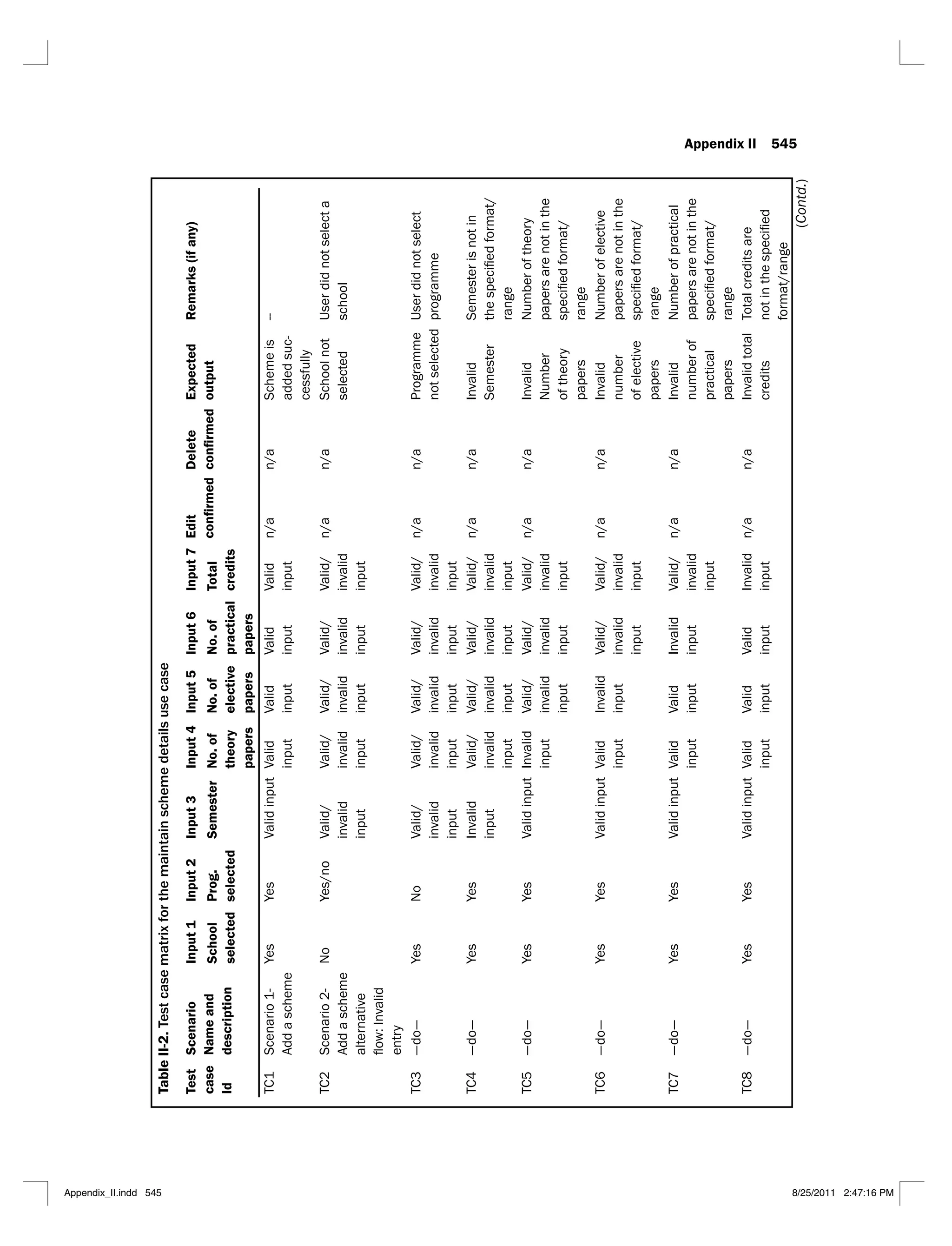
#include<stdio.h>
#include<conio.h>
1. void main()
2. {
3. int mark1, mark2,mark3,avg;
4. clrscr();
5. printf("Enter marks of 3 subjects (between 0-100)n");
6. printf("Enter marks of first subject:");
7. scanf("%d", &mark1);
8. printf("Enter marks of second subject:");
(Contd.)
(Contd.)
Structural Testing 207
9. scanf("%d", &mark2);
10. printf("Enter marks of third subject:");
11. scanf("%d",&mark3);
12. if(mark1>100||mark1<0||mark2>100||mark2<0||mark3>100||mark3<0) { /* do nothing*/
14. }
15. else {
16. avg=(mark1+mark2+mark3)/3;
17. if(avg<40) { /* do nothing*/
19. }
20. else if(avg>=40&&avg<50) {/* do nothing*/
22. }
23. else if(avg>=50&&avg<60) {/* do nothing*/
25. }
26. else if(avg>=60&&avg<75) {/* do nothing*/
28. }
29. else {
30. printf("First Division with Distinction");
31. }
32. }
33. getch();
34. }
(i) S(avg,30)/S(avg,34)
Figure 4.6. Slices of program for determination of division of a student
Table 4.19.
S.
No.
Slice Line covered mark1 mark2 mark3 Expected output
1. S(mark1, 7) 1–7, 34 65 No output
2. S(mark1, 13) 1–14, 33, 34 101 40 50 Invalid marks
3. S(mark1, 34 ) 1–7, 34 65 No output
4. S(mark2, 9) 1–5, 8, 9, 34 65 No output
5. S(mark2, 13) 1–14, 33, 34 40 101 50 Invalid marks
6. S(mark2, 34) 1–5, 8, 9, 34 65 No output
7. S(mark3, 11) 1–5, 10, 11, 34 65 No output
8. S(mark3, 13) 1–14, 33, 34 40 50 101 Invalid marks
(Contd.)
(Contd.)
208 Software Testing
S.
No.
Slice Line covered mark1 mark2 mark3 Expected output
9. S(mark3, 34) 1–5, 10, 11, 34 65 No output
10. S(avg, 16) 1–12, 14–16, 32, 34 45 50 45 No output
11. S(avg, 18) 1–12, 14–19, 32–34 40 30 20 Fail
12. S(avg, 21) 1–12, 14–17, 19–22,
29, 32–34
45 50 45 Third division
13. S(avg, 24) 1–12, 14–17, 19, 20,
22–25, 29, 31–34
55 60 57 Second division
14. S(avg, 27) 1–12, 14–17, 19, 20,
22, 23, 25–29, 31–34
65 67 65 First division
15. S(avg, 30) 1–12, 14–17, 19, 20,
22, 23, 25, 26, 28–34
79 80 85 First division with
distinction
16. S(avg, 34) 1–12, 14–17, 19, 20,
22, 23, 25, 26, 28–34
79 80 85 First division with
distinction
17. S(avg, 16) 1–12, 14–16, 32, 34 45 50 45 No output
Example 4.8: Consider the program for classification of a triangle. Consider all variables and
generate possible program slices. Design at least one test case from every slice.
Solution:
There are seven variables ‘a’, ‘b’, ‘c’, ‘a1’, ‘a2’, ‘a3’and ‘valid’in the program. We may create
many slices as given below:
i. S (a, 8) = {1–8, 42}
ii. S (b, 10) = {1–6, 9, 10, 42}
iii. S (c, 12) = {1–6, 11, 12, 42}
iv. S (a1, 22) = {1–16, 20–22, 34, 42}
v. S (a1, 26) = {1–16, 20–22, 25–27, 34, 41, 42}
vi. S (a1, 29) = {1–16, 20–22, 25, 27–31, 33, 34, 41, 42}
vii. S (a1, 32) = {1–16, 20–22, 25, 27, 28, 30–34, 41, 42}
viii. S (a2, 23) = {1–16, 20, 21,23, 34, 42}
ix. S (a2, 26) = {1–16, 20, 21, 23, 25–27, 34, 41, 42)
x. S (a2, 29) = {1–16, 20, 21, 23, 25, 27–31, 33, 34, 41, 42}
xi. S (a2, 32) = {1–16, 20, 21, 23, 25, 27, 28, 30–34, 41, 42}
xii. S (a3, 26) = {1–16, 20, 21, 24–27, 34, 41, 42}
xiii. S (a3, 29) = {1–16, 20, 21, 24, 25, 27–31, 33, 34, 41,42}
xiv. S (a3, 32) = {1–16, 20, 21, 24, 25, 27, 28, 30–34, 41, 42}
xv. S (valid, 5) = {1–5, 42}
xvi. S (valid, 15) = {1–16, 20, 42}
xvii. S (valid, 18) = {1–14, 16–20, 42}
xviii. S (valid, 36) = {1–14, 16–20, 21, 34–38, 40–42}
xix. S (valid, 39) = {1–13, 20, 21, 34, 35, 37–42}
(Contd.)
Structural Testing 209
The test cases of the above slices are given in Table 4.20.
Table 4.20.
S.
No.
Slice Path a b c Expected output
1. S(a, 8)/S(a,42) 1–8, 42 20 No output
2. S(b, 10)/S(b,42) 1–6, 9, 10, 42 20 No output
3. S(c, 12)/S(c,42) 1–6, 11, 12, 42 20 No output
4. S(a1, 22) 1–16, 20–22, 34, 42 30 20 40 No output
5. S(a1, 26) 1–16, 20–22, 25–27, 34,
41, 42
30 20 40 Obtuse angled
triangle
6. S(a1, 29) 1–16, 20–22, 25, 27–31,
33, 34, 41, 42
30 40 50 Right angled triangle
7. S(a1, 32) 1–16, 20–22, 25, 27, 28,
30–34, 41, 42
50 60 40 Acute angled tri-
angle
8. S(a1, 42) 1–16, 20–22, 34, 42 30 20 40 No output
9. S(a2, 23) 1–16, 20, 21, 23, 34, 42 30 20 40 No output
10. S(a2, 26) 1–16, 20, 21, 23, 25–27,
34, 41, 42
40 30 20 Obtuse angled
triangle
11. S(a2, 29) 1–16, 20, 21, 23, 25,
27–31, 33, 34, 41, 42
50 40 30 Right angled triangle
12. S(a2, 32) 1–16, 20, 21, 23, 25, 27, 28,
30–34, 41, 42
40 50 60 Acute angled tri-
angle
13. S(a2, 42) 1–16, 20, 21, 23, 34, 42 30 20 40 No output
14. S(a3, 24) 1–16, 20, 21, 24, 34, 42 30 20 40 No output
15. S(a3, 26) 1–16, 20, 21, 24–27, 34,
41, 42
20 40 30 Obtuse angled
triangle
16. S(a3, 29) 1–16, 20, 21, 24, 25, 27–31,
33, 34, 41, 42
40 50 30 Right angled triangle
17. S(a3, 32) 1–16, 20, 21, 24, 25, 27, 28,
30–34, 41, 42
50 40 60 Acute angled tri-
angle
18. S(a3, 42) 1–16, 20, 21, 24, 34, 42 30 20 40 No output
19. S(valid,5) 1–2, 5, 42 No output
20. S(valid,15) 1–16, 20, 42 20 40 30 No output
21. S(valid,18) 1–14, 16–20, 42 30 10 15 No output
22. S(valid,36) 1–14, 16–20, 21, 34–38,
40–42
30 10 15 Invalid triangle
23. S(valid,39) 1–13, 20, 21, 34, 35, 37–42 102 –1 6 Input values out of
range
24. S(valid,42) 1–14, 16–20, 42 30 10 15 No output
210 Software Testing
Example 4.9. Consider the program for determination of day of the week given in Figure 3.13.
Consider variables day, validDate, leap and generate possible program slices. Design at least
one test case from each slice.
Solution:
There are ten variables – day, month, year, century Y, Y1, M, date, valid date, and leap. We
may create many slices for variables day, validDate and leap as given below:
1. S(day, 6) = {1–6, 118}
2. S(day, 93) = {1–11, 18–21, 25, 43–48, 53, 54, 61, 62, 69, 70, 72, 73, 75, 76,
78–81, 88, 90–94, 113, 117, 118}
3. S(day, 96) = {1–11, 18–21, 25, 43–48, 53, 54, 61, 62, 69, 70, 72, 73, 75, 76,
78–81, 88, 90–92, 94–97, 110, 112, 113, 117, 118}
4. S(day, 99) = {1–11, 18–21, 25, 43–48, 53, 54, 61, 62, 69, 70, 72, 73, 75, 76,
78–81, 88, 90–92, 94, 95, 97–100, 110, 112, 113, 117, 118}
5. S(day, 102) = {1–11, 18–21, 25, 43–48, 53, 54, 61, 62, 69, 70, 72, 73, 75, 76,
78–81, 88, 90–92, 94, 95, 97, 98, 100–103, 110, 112, 113, 117,
118}
6. S(day, 105) = {1–11, 18–21, 25, 43–48, 53, 54, 61, 62, 69, 70, 72, 73, 75, 76,
78–81, 88, 90–92, 94, 95, 97, 98, 100, 101, 103–106, 110, 112,
113, 117, 118}
7. S(day, 108) = {1–11, 18–21, 25, 43–48, 53, 54, 61, 62, 69, 70, 72, 73, 75, 76,
78–81, 88, 90–92, 94, 95, 97, 98, 100, 101, 103, 104, 106–110,
112, 113, 117, 118}
8. S(day, 111) = {1–11, 18–21, 25, 43–48, 53, 54, 61, 62, 69, 70, 72, 73, 75, 76,
78–81, 88, 90–92, 94, 95, 97, 98, 100, 101, 103, 104, 106, 107,
109–113, 117, 118}
9. S(day, 115) = {1–11, 43, 44, 113–118}
10. S(day, 118) = {1–6, 118}
11. S(validDate,3) = {1–3, 118}
12. S(validDate,20) = {1–11, 18–21, 25, 43, 118}
13. S(validDate,23) = {1–11, 18, 19, 21–25, 43, 118}
14. S(validDate,28) = {1–13, 17, 18, 25, 26–29, 36, 40, 42, 43, 118}
15. S(validDate,31) = {1–11, 18, 25, 26, 27, 29–33, 35, 36, 40, 42, 43, 118}
16. S(validDate,34) = {1–11, 18, 25, 26, 27, 29, 30, 32–36, 40, 42, 43, 118}
17.. S(validDate,38) = {1–11, 18, 25, 26, 36–40, 42, 43, 118}
18. S(validDate,41) = {1–11, 18, 25, 26, 36, 37, 39–43, 118}
19. S(validDate,118) = {1–11, 18, 25, 26, 36, 37, 39–43, 118}
20. S(leap,3) = {1–3, 118}
21. S(leap,13) = {1–13, 17, 43, 118}
22. S(leap,15) = {1–17, 43, 118}
23. S(leap,118) = {1–17, 43, 118}
Structural Testing 211
The test cases for the above slices are given in Table 4.21.
Table 4.21.
S.
No.
Slice Lines covered Month Day Year
Expected
output
1. S(day, 6) 1–6, 118 6 - - No output
2. S(day, 93) 1–11, 18–21, 25, 43–48, 53,
54, 61, 62, 69, 70, 72, 73, 75,
76, 78–81, 88, 90–94, 113,
117, 118
6 13 1999 Sunday
3. S(day, 96) 1–11, 18–21, 25, 43–48, 53,
54, 61, 62, 69, 70, 72, 73, 75,
76, 78–81, 88, 90–92, 94–97,
110, 112, 113, 117, 118
6 14 1999 Monday
4. S(day, 99) 1–11, 18–21, 25, 43–48, 53,
54, 61, 62, 69, 70, 72, 73, 75,
76, 78–81, 88, 90–92, 94, 95,
97–100, 110, 112, 113, 117,
118
6 15 1999 Tuesday
5. S(day, 102) 1–11, 18–21, 25, 43–48, 53,
54, 61, 62, 69, 70, 72, 73, 75,
76, 78–81, 88, 90–92, 94, 95,
97, 98, 100–103, 110, 112,
113, 117, 118
6 16 1999 Wednesday
6. S(day, 105) 1–11, 18–21, 25, 43–48, 53,
54, 61, 62, 69, 70, 72, 73, 75,
76, 78–81, 88, 90–92, 94, 95,
97, 98, 100, 101, 103–106,
110, 112, 113, 117, 118
6 17 1999 Thursday
7. S(day, 108) 1–11, 18–21, 25, 43–48, 53,
54, 61, 62, 69, 70, 72, 73, 75,
76, 78–81, 88, 90–92, 94, 95,
97, 98, 100, 101, 103, 104,
106–110, 112, 113, 117, 118
6 18 1999 Friday
8. S(day, 111) 1–11, 18–21, 25, 43–48, 53,
54, 61, 62, 69, 70, 72, 73, 75,
76, 78–81, 88, 90–92, 94, 95,
97, 98, 100, 101, 103, 104,
106, 107, 109–113, 117, 118
6 19 1999 Saturday
9. S(day, 115) 1–11, 43, 44, 113–118 6 31 2059 Invalid Date
10. S(day, 118) 1–6, 118 6 19 1999 Saturday
11. S(validDate,3) 1–3, 118 - - - No output
12. S(validDate,20) 1–11, 18–21, 25, 43, 118 6 15 2009 No output
13. S(validDate,23) 1–11, 18, 19, 21–25, 43, 118 6 31 2009 No output
14. S(validDate,28) 1–13, 17, 18, 25, 26–29, 36,
40, 42, 43, 118
2 15 2000 No output
(Contd.)
212 Software Testing
S.
No.
Slice Lines covered Month Day Year
Expected
output
15. S(validDate,31) 1–11, 18, 25, 26, 27, 29–33,
35, 36, 40, 42, 43, 118
2 15 2009 No output
16. S(validDate,34) 1–11, 18, 25, 26, 27, 29, 30,
32–36, 40, 42, 43, 118
2 29 2009 No output
17. S(validDate,38) 1–11, 18, 25, 26, 36–40, 42,
43, 118
8 15 2009 No output
18. S(validDate,41) 1–11, 18, 25, 26, 36, 37,
39–43, 118
13 15 2009 No output
19. S(validDate,118) 1–11, 18, 25, 26, 36, 37,
39–43, 118
13 15 2009 No output
20. S(leap,3) 1–3, 118 - - - No output
21. S(leap,13) 1–13, 17, 43, 118 8 15 2000 No output
22. S(leap,15) 1–17, 43, 118 8 15 1900 No output
23. S(leap,118) 1–17, 43, 118 8 15 1900 No output
4.4 MUTATION TESTING
It is a popular technique to assess the effectiveness of a test suite. We may have a large number
of test cases for any program. We neither have time nor resources to execute all of them. We
may select a few test cases using any testing technique and prepare a test suite. How do we
assess the effectiveness of a selected test suite? Is this test suite adequate for the program? If
the test suite is not able to make the program fail, there may be one of the following reasons:
The test suite is effective but hardly any errors are there in the program. How will a test
(i)
suite detect errors when they are not there?
The test suite is not effective and could not find any errors. Although there may be
(ii)
errors, they could not be detected due to poor selection of test suite. How will errors be
detected when the test suite is not effective?
In both the cases, we are not able to find errors, but the reasons are different. In the first
case, the program quality is good and the test suite is effective and in the second case, the
program quality is not that good and the test suite is also not that effective. When the test suite
is not able to detect errors, how do we know whether the test suite is not effective or the
program quality is good? Hence, assessing the effectiveness and quality of a test suite is very
important. Mutation testing may help us to assess the effectiveness of a test suite and may also
enhance the test suite, if it is not adequate for a program.
4.4.1 Mutation and Mutants
The process of changing a program is known as mutation. This change may be limited to one,
two or very few changes in the program. We prepare a copy of the program under test and make
a change in a statement of the program. This changed version of the program is known as a
(Contd.)
Structural Testing 213
mutant of the original program. The behaviour of the mutant may be different from the original
program due to the introduction of a change. However, the original program and mutant are
syntactically correct and should compile correctly. To mutate a program means to change a
program. We generally make only one or two changes in order to assess the effectiveness of
the selected test suite. We may make many mutants of a program by making small changes in
the program. Every mutant will have a different change in a program. Consider a program to
find the largest amongst three numbers as given in Figure 3.11 and its two mutants are given
in Figure 4.7 and Figure 4.8. Every change of a program may give a different output as
compared to the original program.
Many changes can be made in the program given in Figure 3.11 till it is syntactically
correct. Mutant M1
is obtained by replacing the operator ‘>’ of line number 11 by the operator
‘ =’. Mutant M2
is obtained by changing the operator ‘>’ of line number 20 to operator ‘<’.
These changes are simple changes. Only one change has been made in the original program to
obtain mutant M1
and mutant M2
.
#include<stdio.h>
#include<conio.h>
1. void main()
2. {
3. float A,B,C;
4. clrscr();
5. printf("Enter number 1:n");
6. scanf("%f", &A);
7. printf("Enter number 2:n");
8. scanf("%f", &B);
9. printf("Enter number 3:n");
10. scanf("%f", &C);
/*Check for greatest of three numbers*/
11. if(A=B) { mutated statement (‘>’ is replaced by ‘=’)
12. if(A>C) {
13. printf("The largest number is: %fn",A);
14. }
15. else {
16. printf("The largest number is: %fn",C);
17. }
18. }
19. else {
20. if(C>B) {
21. printf("The largest number is: %fn",C);
22. }
23. else {
24. printf("The largest number is: %fn",B);
25. }
26. }
if(A>B){
(Contd.)
214 Software Testing
27. getch();
28. }
M1
: First order mutant
Figure 4.7. Mutant1
(M1
) of program to find the largest among three numbers
#include<stdio.h>
#include<conio.h>
1. void main()
2. {
3. float A,B,C;
4. clrscr();
5. printf("Enter number 1:n");
6. scanf("%f", &A);
7. printf("Enter number 2:n");
8. scanf("%f", &B);
9. printf("Enter number 3:n");
10. scanf("%f", &C);
/*Check for greatest of three numbers*/
11. if(A>B) {
12. if(A>C) {
13. printf("The largest number is: %fn",A);
14. }
15. else {
16. printf("The largest number is: %fn",C);
17. }
18. }
19. else {
20. if(C<B) { mutated statement (‘>’ is replaced by ‘<’)
21. printf("The largest number is: %fn",C);
22. }
23. else {
24. printf("The largest number is: %fn",B);
25. }
26. }
27. getch();
28. }
M2
: First order mutant
Figure 4.8. Mutant2
(M2
) of program to find the largest among three numbers
if(C>B) {
(Contd.)
Structural Testing 215
The mutants generated by making only one change are known as first order mutants. We may
obtain second order mutants by making two simple changes in the program and third order mutants
by making three simple changes, and so on. The second order mutant (M3
) of the program given in
Figure 3.11 is obtained by making two changes in the program and thus changing operator ‘>’ of
line number 11 to operator ‘<’and operator ‘>’of line number 20 to ‘ ’as given in Figure 4.9. The
second order mutants and above are called higher order mutants. Generally, in practice, we prefer
to use only first order mutants in order to simplify the process of mutation.
#include<stdio.h>
#include<conio.h>
1. void main()
2. {
3. float A,B,C;
4. clrscr();
5. printf("Enter number 1:n");
6. scanf("%f", &A);
7. printf("Enter number 2:n");
8. scanf("%f", &B);
9. printf("Enter number 3:n");
10. scanf("%f", &C);
/*Check for greatest of three numbers*/
11. if(A<B) { mutated statement (replacing ‘>’ by ‘<’)
12. if(A>C) {
13. printf("The largest number is: %fn",A);
14. }
15. else {
16. printf("The largest number is: %fn",C);
17. }
18. }
19. else {
20. if(C B) { mutated statement (replacing ‘>’by ‘ ’)
21. printf("The largest number is: %fn",C);
22. }
23. else {
24. printf("The largest number is: %fn",B);
25. }
26. }
27. getch();
28. }
M3
: Second order mutant
Figure 4.9. Mutant3
(M3
) of program to find the largest among three numbers
if(A>B) {
if(C>B) {
216 Software Testing
4.4.2 Mutation Operators
Mutants are produced by applying mutant operators. An operator is essentially a grammatical
rule that changes a single expression to another expression. The changed expression should be
grammatically correct as per the used language. If one or more mutant operators are applied to
all expressions of a program, we may be able to generate a large set of mutants. We should
measure the degree to which the program is changed. If the original expression is x + 1, and
the mutant for that expression is x + 2, that is considered as a lesser change as compared to a
mutant where the changed expression is (y * 2) by changing both operands and the operator.
We may have a ranking scheme, where a first order mutant is a single change to an expression,
a second order mutant is a mutation to a first order mutant, and so on. Higher order mutants
become difficult to manage, control and trace. They are not popular in practice and first order
mutants are recommended to be used. To kill a mutant, we should be able to execute the
changed statement of the program. If we are not able to do so, the fault will not be detected. If
x – y is changed to x – 5 to make a mutant, then we should not use the value of y to be equal
to 5. If we do so, the fault will not be revealed. Some of the mutant operators for object
oriented languages like Java, C++ are given as:
Changing the access modifier, like public to private.
(i)
Static modifier change
(ii)
Argument order change
(iii)
Super Keyword change
(iv)
Operator change
(v)
Any operand change by a numeric value.
(vi)
4.4.3 Mutation Score
When we execute a mutant using a test suite, we may have any of the following outcomes:
The results of the program are affected by the change and any test case of the test suite
(i)
detects it. If this happens, then the mutant is called a killed mutant.
The results of the program are not affected by the change and any test case of the test
(ii)
suite does not detect the mutation. The mutant is called a live mutant.
The mutation score associated with a test suite and its mutants is calculated as:
Mutation Score
Number of mutants killed
Total number of mut
tants
The total number of mutants is equal to the number of killed mutants plus the number of
live mutants. The mutation score measures how sensitive the program is to the changes and
how accurate the test suite is. A mutation score is always between 0 and 1. A higher value of
mutation score indicates the effectiveness of the test suite although effectiveness also depends
on the types of faults that the mutation operators are designed to represent.
The live mutants are important for us and should be analyzed thoroughly. Why is it that any
test case of the test suite not able to detect the changed behaviour of the program? One of the
reasons may be that the changed statement was not executed by these test cases. If executed,
Structural Testing 217
then also it has no effect on the behaviour of the program. We should write new test cases for
live mutants and kill all these mutants. The test cases that identify the changed behaviour
should be preserved and transferred to the original test suite in order to enhance the capability
of the test suite. Hence, the purpose of mutation testing is not only to assess the capability of
a test suite but also to enhance the test suite. Some mutation testing tools are also available in
the market like Insure++, Jester for Java (open source) and Nester for C++ (open source).
Example 4.10: Consider the program to find the largest of three numbers as given in figure
3.11. The test suite selected by a testing technique is given as:
S. No. A B C Expected Output
1. 6 10 2 10
2. 10 6 2 10
3. 6 2 10 10
4. 6 10 20 20
Generate five mutants (M1
to M5
) and calculate the mutation score of this test suite.
Solution:
The mutated line numbers and changed lines are shown in Table 4.22.
Table 4.22. Mutated statements
Mutant No. Line no. Original line
M1
11 if(A>B) if (A<B)
M2
11 if(A>B) if(A>(B+C))
M3
12 if(A>C) if(A<C)
M4
20 if(C>B) if(C=B)
M5
16 printf(“The Largest number
is:%fn”,C);
printf(“The Largest number
is:%fn”,B);
The actual output obtained by executing the mutants M1
-M5
is shown in Tables 4.23-4.27.
Table 4.23. Actual output of mutant M1
Test case A B C Expected output Actual output
1. 6 10 2 10 6
2. 10 6 2 10 6
3. 6 2 10 10 10
4. 6 10 20 20 20
Table 4.24. Actual output of mutant M2
Test case A B C Expected output Actual output
1. 6 10 2 10 10
2. 10 6 2 10 10
3. 6 2 10 10 10
4. 6 10 20 20 20
218 Software Testing
Table 4.25. Actual output of mutant M3
Test case A B C Expected output Actual output
1. 6 10 2 10 10
2. 10 6 2 10 2
3. 6 2 10 10 6
4. 6 10 20 20 20
Table 4.26. Actual output of mutant M4
Test case A B C Expected output Actual output
1. 6 10 2 10 10
2. 10 6 2 10 10
3. 6 2 10 10 10
4. 6 10 20 20 10
Table 4.27. Actual output of mutant M5
Test case A B C Expected output Actual output
1. 6 10 2 10 10
2. 10 6 2 10 10
3. 6 2 10 10 2
4. 6 10 20 20 20
Mutation Score
Number of mutants killed
Total number of muta
ants
4
5
0 8
.
Higher the mutant score, better is the effectiveness of the test suite. The mutant M2
is live
in the example. We may have to write a specific test case to kill this mutant. The additional test
case is given in Table 4.28.
Table 4.28.
Test case A B C Expected output
5. 10 5 6 10
Now when we execute the test case 5, the actual output will be different from the expected
output (see Table 4.29), hence the mutant will be killed.
Table 4.29. Output of added test case
Test case A B C Expected output Actual output
5. 10 5 6 10 6
Structural Testing 219
This test case is very important and should be added to the given test suite. Therefore, the
revised test suite is given in Table 4.30.
Table 4.30.
Test case A B C Expected output
1. 6 10 2 10
2. 10 6 2 10
3. 6 2 10 10
4. 6 10 20 20
5. 10 5 6 10
Example 4.11: Consider the program for classification of triangle given in Figure 3.18. The
test suite A and B are selected by two different testing techniques and are given in Table 4.31
and Table 4.32, respectively. The five first order mutants and the modified lines are given in
Table 4.33. Calculate the mutation score of each test suite and compare their effectiveness.
Also, add any additional test case, if required.
Table 4.31.
Test case a b c Expected output
1. 30 40 90 Invalid triangle
2. 30 20 40 Obtuse angled triangle
3. 50 40 60 Acute angled triangle
4. 30 40 50 Right angled triangle
5. –1 50 40 Input values are out of range
6. 50 150 90 Input values are out of range
7. 50 40 –1 Input values are out of range
Table 4.32.
Test case a b c Expected output
1. 40 90 20 Invalid triangle
2. 40 30 60 Obtuse angled triangle
3. 40 50 60 Acute angled triangle
4. 30 40 50 Right angled triangle
5. –1 50 40 Input values are out of range
6. 30 101 90 Input values are out of range
7. 30 90 0 Input values are out of range
Table 4.33.
Mutant
No.
Line
no.
Original line
M1
13 if(a>0&&a<=100&&b>0&&b<=10
0&&c>0&&c<=100) {
if(a>0||a<=100&&b>0&&b<=100&
&c>0&&c<=100) {
M2
14 if((a+b)>c&&(b+c)>a&&(c+a)>b) { if((a+b)>c&&(b+c)>a&&(b+a)>b) {
M3
21 if(valid==1) { if(valid>1) {
M4
23 a2=(b*b+c*c)/(a*a); a2=(b*b+c*c)*(a*a);
M5
25 if(a1<1||a2<1||a3<1) { if(a1>1||a2<1||a3<1) {
220 Software Testing
Solution:
The actual outputs of mutants M1
-M5
on test suite A are shown in Tables 4.34-4.38.
Table 4.34. Actual output of M1
(A)
Test case a b c Expected output Actual output
1. 30 40 90 Invalid triangle Invalid triangle
2. 30 20 40 Obtuse angled triangle Obtuse angled triangle
3. 50 40 60 Acute angled triangle Acute angled triangle
4. 30 40 50 Right angled triangle Right angled triangle
5. –1 50 40 Input values are out of range Invalid triangle
6. 50 150 90 Input values are out of range Invalid triangle
7. 50 40 –1 Input values are out of range Invalid triangle
Table 4.35. Actual output of M2
(A)
Test case a b c Expected output Actual output
1. 30 40 90 Invalid triangle Invalid triangle
2. 30 20 40 Obtuse angled triangle Obtuse angled triangle
3. 50 40 60 Acute angled triangle Acute angled triangle
4. 30 40 50 Right angled triangle Right angled triangle
5. –1 50 40 Input values are out of range Input values are out of range
6. 50 150 90 Input values are out of range Input values are out of range
7. 50 40 –1 Input values are out of range Input values are out of range
Table 4.36. Actual output of M3
(A)
Test case a b c Expected output Actual output
1. 30 40 90 Invalid triangle Invalid triangle
2. 30 20 40 Obtuse angled triangle Input values are out of range
3. 50 40 60 Acute angled triangle Input values are out of range
4. 30 40 50 Right angled triangle Input values are out of range
5. –1 50 40 Input values are out of range Input values are out of range
6. 50 150 90 Input values are out of range Input values are out of range
7. 50 40 –1 Input values are out of range Input values are out of range
Table 4.37. Actual output of M4
(A)
Test case a b c Expected output Actual output
1. 30 40 90 Invalid triangle Invalid triangle
2. 30 20 40 Obtuse angled triangle Obtuse angled triangle
3. 50 40 60 Acute angled triangle Acute angled triangle
4. 30 40 50 Right angled triangle Right angled triangle
5. –1 50 40 Input values are out of range Input values are out of range
6. 50 150 90 Input values are out of range Input values are out of range
7. 50 40 –1 Input values are out of range Input values are out of range
Structural Testing 221
Table 4.38. Actual output of M5
(A)
Test case a b c Expected output Actual output
1. 30 40 90 Invalid triangle Invalid triangle
2. 30 20 40 Obtuse angled triangle Acute angled triangle
3. 50 40 60 Acute angled triangle Obtuse angled triangle
4. 30 40 50 Right angled triangle Right angled triangle
5. –1 50 40 Input values are out of range Input values are out of range
6. 50 150 90 Input values are out of range Input values are out of range
7. 50 40 –1 Input values are out of range Input values are out of range
Two mutants are M2
and M4
are live. Thus, the mutation score using test suite A is 0.6.
Mutation Score
Number of mutants killed
Total number of mut
tants
3
5
0 6
.
The actual outputs of mutants M1
-M5
on test suite B are shown in Tables 4.39-4.43.
Table 4.39. Actual output of M1
Test case a b c Expected output Actual output
1. 40 90 20 Invalid triangle Invalid triangle
2. 40 30 60 Obtuse angled triangle Obtuse angled triangle
3. 40 50 60 Acute angled triangle Acute angled triangle
4. 30 40 50 Right angled triangle Right angled triangle
5. –1 50 40 Input values are out of range Invalid triangle
6. 30 101 90 Input values are out of range Obtuse angled triangle
7. 30 90 0 Input values are out of range Invalid triangle
Table 4.40. Actual output of M2
Test case a b c Expected output Actual output
1. 40 90 20 Invalid triangle Obtuse angled triangle
2. 40 30 60 Obtuse angled triangle Obtuse angled triangle
3. 40 50 60 Acute angled triangle Acute angled triangle
4. 30 40 50 Right angled triangle Right angled triangle
5. –1 50 40 Input values are out of range Input values are out of range
6. 30 101 90 Input values are out of range Input values are out of range
7. 30 90 0 Input values are out of range Input values are out of range
222 Software Testing
Table 4.41. Actual output of M3
Test case a b c Expected output Actual output
1. 40 90 20 Invalid triangle Invalid triangle
2. 40 30 60 Obtuse angled triangle Input values are out of range
3. 40 50 60 Acute angled triangle Input values are out of range
4. 30 40 50 Right angled triangle Input values are out of range
5. –1 50 40 Input values are out of range Input values are out of range
6. 30 101 90 Input values are out of range Input values are out of range
7. 30 90 0 Input values are out of range Input values are out of range
Table 4.42. Actual output of M4
Test case a b c Expected output Actual output
1. 40 90 20 Invalid triangle Invalid triangle
2. 40 30 60 Obtuse angled triangle Obtuse angled triangle
3. 40 50 60 Acute angled triangle Acute angled triangle
4. 30 40 50 Right angled triangle Right angled triangle
5. –1 50 40 Input values are out of range Input values are out of range
6. 30 101 90 Input values are out of range Input values are out of range
7. 30 90 0 Input values are out of range Input values are out of range
Table 4.43. Actual output of M5
Test case a b c Expected output Actual output
1. 40 90 20 Invalid triangle Invalid triangle
2. 40 30 60 Obtuse angled triangle Acute angled triangle
3. 40 50 60 Acute angled triangle Obtuse angled triangle
4. 30 40 50 Right angled triangle Right angled triangle
5. –1 50 40 Input values are out of range Input values are out of range
6. 30 101 90 Input values are out of range Input values are out of range
7. 30 90 0 Input values are out of range Input values are out of range
Mutation Score
Number of mutants killed
Total number of muta
ants
4
5
0 8
.
The mutation score of Test suite B is higher as compared to the mutation score of test suite
A, hence test suite B is more effective in comparison to test suite A. In order to kill the live
mutant (M4
), an additional test case should be added to test suite B as shown in Table 4.44.
Table 4.44.
Test case a b c Expected output
8. 40 30 20 Obtuse angled triangle
Structural Testing 223
The revised test suite B is given in Table 4.45.
Table 4.45.
Test case a b c Expected output
1. 40 90 20 Invalid triangle
2. 40 30 60 Obtuse angled triangle
3. 40 50 60 Acute angled triangle
4. 30 40 50 Right angled triangle
5. –1 50 40 Input values are out of range
6. 30 101 90 Input values are out of range
7. 30 90 0 Input values are out of range
8. 40 30 20 Obtuse angled triangle
MULTIPLE CHOICE QUESTIONS
Note: Select the most appropriate answer for the following questions.
Which is not a structural testing technique?
4.1
Mutation testing
(a)
Data flow testing
(b)
Slice based testing
(c)
Decision table based testing
(d)
Which is a structural testing technique?
4.2
Data flow testing
(a)
Control flow testing
(b)
Mutation testing
(c)
All of the above
(d)
Data flow testing is related to:
4.3
ER diagrams
(a)
Data flow diagrams
(b)
Data dictionaries
(c)
None of the above
(d)
Mutation testing is related to:
4.4
Fault seeding
(a)
Fault severity
(b)
Fault impact analysis
(c)
None of the above
(d)
Mutation score does not indicate anything about:
4.5
Size of a test suite
(a)
Effectiveness of a test suite
(b)
Performance of a test suite
(c)
Usefulness of a test suite
(d)
224 Software Testing
100% statement coverage and branch coverage means:
4.6
Every statement has been tested
(a)
Every outcome of a branch statement has been tested
(b)
Every statement and every branch has been tested
(c)
Every condition has been tested
(d)
How many test cases are required for 100% statement and branch coverage of the
4.7
following source code?
void main ( )
{
int a, b;
scanf (“%d”, &a);
scanf (“%d”, &b);
if (a>b) {
printf (“a is large”);
}
else {
printf (“b is large”);
}
}
1 test case for statement coverage, 2 for branch coverage.
(a)
2 test case for statement coverage, 1 for branch coverage.
(b)
2 test case for statement coverage, 2 for branch coverage.
(c)
1 test case for statement coverage, 3 for branch coverage.
(d)
Which of the following statements about the relationship of statement coverage and
4.8
decision coverage is correct?
100% statement coverage means 100% decision coverage.
(a)
100% decision coverage means 100% statement coverage.
(b)
90% statement coverage means 90% decision coverage.
(c)
90% decision coverage means 90% statement coverage.
(d)
In data flow testing, which criterion generates the maximum number of test cases?
4.9
Test all du-paths
(a)
Test all uses
(b)
Test all definitions
(c)
All of the above generates the same number of test cases
(d)
Statements coverage will not check for :
4.10
Missing statements
(a)
Extra statements
(b)
Dead statements
(c)
Unused statements
(d)
Statement coverage is commonly used to measure:
4.11
Test effectiveness
(a)
Number of faults
(b)
Testing time
(c)
Complexity of code
(d)
Structural Testing 225
Structural testing techniques may help us to:
4.12
Understand the source code
(a)
Generate test cases using various paths
(b)
Comprehend the program
(c)
All of the above
(d)
A program slice is:
4.13
More complex than the original program
(a)
Larger than the original program
(b)
Smaller than the original program
(c)
More critical than the original program
(d)
Which mutants are more popular in practice?
4.14
First order mutant
(a)
Second order mutant
(b)
Third order mutant
(c)
Zero order mutant
(d)
Source code coverage measurement is :
4.15
A partial measure of test effectiveness
(a)
Not related to testing
(b)
Easily achievable in practice
(c)
None of the above
(d)
Which of the following is not related?
4.16
White box
(a)
Black box
(b)
Glass box
(c)
Structural
(d)
Mutation score is related to:
4.17
Effectiveness of a test suite
(a)
Size of a test suite
(b)
Complexity of a test suite
(c)
Criticality of a test suite
(d)
Which is a mutation testing tool?
4.18
Insure++
(a)
Jester for Java
(b)
Nester for c++
(c)
All of the above
(d)
Which is difficult to achieve?
4.19
100% statement coverage
(a)
100% branch coverage
(b)
100% condition coverage
(c)
100% path coverage
(d)
Program slicing was introduced by:
4.20
Mark Weiser
(a)
Victor Basili
(b)
L. Briand
(c)
Mc Cabe
(d)
226 Software Testing
EXERCISES
What is structural testing? How is it different from functional testing?
4.1
What are different types of structural testing techniques? Discuss any two techniques
4.2
with the help of examples.
Discuss the significance of path testing. How can we make it more effective?
4.3
Show with the help of an example that a very high level of statement coverage does
4.4
not mean that the program is defect-free.
Write a program to find roots of a quadratic equation.
4.5
Draw program graph, DD path graph. Also find independent paths and generate
(a)
test cases.
Find all du-paths and identify those du-paths that are not dc paths. Write test cases
(b)
for every du-path.
Explain define/use testing. Consider the NextDate function and write a program in ‘C’
4.6
language. Find all du paths and dc paths. Design test cases for every definition to every
usage.
Consider a program for classification of a triangle. Its input is a triple of positive integers
4.7
(say a, b and c) from interval [1, 100]. The output may be one of the following:
[Scalene, Isosceles, Equilateral, Not a triangle, invalid inputs]
Draw a program graph, DD path graph and write test cases for every independent
(a)
path.
Find all du-paths and identify those du-paths that are not dc paths. Write test cases
(b)
for every du-path.
What is slice based testing? How can it improve testing? Explain the concept with the
4.8
help of an example and write test cases accordingly.
What is mutation testing? What is the purpose of mutation score? Why are higher order
4.9
mutants not preferred?
Differentiate between black box and white box testing. Consider a program to find the
4.10
largest number amongst three numbers. Generate test cases using one black box testing
and one white box testing technique.
How is data flow testing performed? Is it possible to design data flow test cases
4.11
manually? Justify your answer.
What do you mean by a program graph? What is its use? How can we use it in the
4.12
design of du-paths?
Write a program to print the grade of a student according to the following criteria:
4.13
marks > 80 A+ Grade
(i)
70 < marks
(ii) 80 A Grade
60 < marks
(iii) 70 B Grade
50 < marks
(iv) 60 C Grade
40 < marks
(v) 50 D Grade
Generate all du-paths and write test cases for all du-paths.
Consider the program given below. Find all du-paths and identify those du-paths that
4.14
are definition clear. Also find all du-paths, all-uses and all-definitions and generate test
cases for these paths.
Structural Testing 227
/* Program to calculate total telephone bill amount to be paid by an customer*/
#include<stdio.h>
#include<conio.h>
1. void main()
2. {
3. int custnum,numcalls,valid=0;
4. float netamount;
5. clrscr();
6. printf("Enter customer number & number of calls:");
7. scanf("%d %d",&custnum,&numcalls);
8. if(custnum>10&&custnum<20000){
9. valid=1;
10. if(numcalls<0){
11. valid=-1;
12. }
13. }
14. if(valid==1){
15. if(numcalls<76){
16. netamount=500;
17. }
18. else if(numcalls>75&&numcalls<201){
19. netamount=500+0.80*(numcalls-75);
20. }
21. else if(numcalls>200&&numcalls<501){
22. netamount=500+1.00*(numcalls-200);
23. }
24. else{
25. netamount=500+1.20*(numcalls-500);
26. }
27. printf("nCustomer number: %dt Total Charges:%.3f",custnum,netamount);
28. }
29. else if(valid==0){
30. printf("Invalid customer number");
31. }
32. else{
33. printf("Invalid number of calls");
34. }
35. getch();
36. }
Consider the program for determination of the total telephone bill amount to be paid
4.15
by a customer given in exercise 4.14. Consider all variables and generate possible
program slices. Design at least one test case from every slice.
228 Software Testing
Consider the program for determination of the total telephone bill amount to be paid
4.16
by a customer given in exercise 4.14. Generate two first order mutants and one second
order mutant. Design a test suite of five test cases and calculate the mutation score of
the test suite.
Consider a program to input two numbers and print them in ascending order given
4.17
below. Find all du-paths and identify those du-paths that are definition clear. Also find
all du-paths, all-uses and all-definitions and generate test cases for these paths.
#include<stdio.h>
#include<conio.h>
1. void main()
2. {
3. int a,b,t;
4. clrscr();
5. printf("Enter first number:");
6. scanf("%d",&a);
7. printf("Enter second number:");
8. scanf("%d",&b);
9. if(a<b){
10. t=a;
11. a=b;
12. b=t;
13. }
14. printf("%d %d",a,b);
15. getch();
16. }
Consider a program to input two numbers and print them in ascending order given in
4.18
exercise 4.17. Consider all variables and generate possible program slices. Design at
least one test case from every slice.
Establish the relationship between data flow testing and slice based testing.
4.19
What is the importance of mutation testing? Why is it becoming popular?
4.20
FURTHER READING
Copeland’s book provides introduction to levels of converge:
Lee Copeland, “A Practitioner’s Guide to Software Test Design”, Artech House,
2004.
Key concepts and definitions for structural data flow testing are given by Weyuker:
Weyuker, Elaine J. “Data Flow Testing”, In MARC94, pp. 247–249.
The research paper explains the basic concepts of data flow testing with an example:
J. Badlaney R. Ghatol R. Jadhwani, “An Introduction to Data-Flow Testing”,
TR-2006-22, 2006.
Structural Testing 229
An edited tutorial on testing and collection of important publications may be found
in:
T.J. McCabe, “Structured Testing”, Silver Spring, M.D, IEEE Computer Society
Press, 1982.
Path covering changes and issues are found in:
S.C.Ntafos,“AGraphTheoreticApproachtoProgramTesting”,Ph.DDissertation,
Northwestern University, 1978.
Some important issues of complexity of data flow testing are discussed in:
E.J. Weyuker, “An Empirical Study of the Complexity of Data Flow Testing”,
Second Workshop on Software Testing, Verification and Analysis, Banff, Canada,
pp. 19–21, July 1988.
A comparison of du-paths and branch coverage metrics can be found in:
M.D. Weiser, J.D. Gannon and P.R. McMullin, “Comparison of Structural Test
Coverage Metrics,” IEEE Software, vol. 2, pp. 80–85, March 1985.
Weiser was probably the first one to introduce program slicing:
M. Weiser, “Program Slicing”, Proceedings of the Fifth International Conference
on Software Engineering pp. 439–449, March 1981.
M. Weiser, “Programmers use Slices when Debugging”, Communications of ACM,
vol. 25, no. 7, pp. 446–452, 1982.
M. Weiser, “Program Slicing”, IEEE Transactions on Software Engineering,
SE-10, pp. 352–357, 1984.
Dasso provides an introduction to mutation testing in Chapter 7 of the book:
Aristides Dasso, Ana Funes, “Verification, Validation and Testing in Software
Engineering”, Idea Group Inc, 2007.
The following research paper provides a comprehensive analysis and survey on
mutation testing:
Yue Jia, Mark Harman, “An Analysis and Survey of the Development of Mutation
Testing”, CREST Centre, King’s College London, Technical Report TR-09-06.
http://www.dcs.kcl.ac.uk/pg/jiayue/repository/TR-09-06.pdf, September 2009.
A publicly available repository that provides complete literature on mutation testing
can accessed from:
http://www.dcs.kcl.ac.uk/pg/jiayue/repository/
Other useful research papers may be:
S. Rapps and E.J. Weyuker, “Selecting Software Test Data Using Data Flow
Information”, IEEE Transactions on Software Engineering, vol. 11, no. 4, pp.
367–375, 1985.
K.C. Tai, “What to do beyond Branch Testing,” ACM SIGSOFT Software
Engineering Notes, vol. 14, no. 2, pp. 58–61, April 1989.
A. J. Offutt and D. Lee Stephen, “An Empirical Evaluation of Weak Mutation”, IEEE
Transactions on Software Engineering, vol. 20, no. 5, pp. 337–344, May 1994.
A. Watson, T.J. McCabe, “Structured Testing: A Testing Methodology Using the
Cyclomatic Complexity Metric”, NIST, 1996.
A. J. Offutt and J. Pan, “Detecting Equivalent Mutants and the Feasible Path
Problem”, Software Testing, Verification, and Reliability, vol. 7, no. 3, pp.
165–192, September 1997.
5
Software verification has proved its effectiveness in the software world and its usage is
increasing day by day. The most important aspect of software verification is its implementation
in the early phases of the software development life cycle. There was a time when people used
to say that “testing is a post-mortem activity where testers are only finding the damages already
been done and making changes in the program to get rid of these damages.” Testing primarily
used to be validation oriented where the program was required for execution and was available
only in the later phases of software development. Any testing activity which requires program
execution comes under the ‘validation’ category. In short, whenever we execute the program
with its input(s) and get output(s), that type of testing is known as software validation.
What is software verification? How can we apply this in the early phases of software
development? If we review any document for the purpose of finding faults, it is called verification.
Reviewing a document is possible from the first phase of software development i.e. software
requirement and analysis phase where the end product is the SRS document.
Verification is the process of manually examining / reviewing a document. The document may
be SRS, SDD, the program itself or any document prepared during any phase of software
development. We may call this as static testing because the execution of the program is not
required. We evaluate, review and inspect documents which are generated after the completion
of every phase of software development. As per IEEE, “verification is the process of evaluating
the system or component to determine whether the products of a given development phase satisfy
the conditions imposed at the start of that phase” [IEEE01]. Testing includes both verification and
validation activities and they are complementary to each other. If effective verification is carried
out, we may detect a number of faults in the early phases of the software development life cycle
and ultimately may be able to produce a quality product within time and budget.
5.1 VERIFICATION METHODS
The objective of any verification method is to review the documents with the purpose of finding
faults. Many methods are commonly used in practice like peer reviews, walkthroughs, inspections,
etc. Verification helps in prevention of potential faults, which may lead to failure of software.
After the completion of the implementation phase, we start testing the program by executing it.
We may carry out verification also by reviewing the program manually and examining the critical
areas carefully. Verification and validation activities may be performed after the implementation
phase. However, only verification is possible in the phases prior to implementation like the
requirement phase, the design phase and even most of the implementation phase.
5.1.1 Peer Reviews
Any type of testing (verification or validation), even adhoc and undisciplined, is better than no
testing if it is carried out by person(s) other than the developers / writers of the document with
the purpose of finding faults. This is the simplest way of reviewing the documents / programs
to find out faults during verification. We give the document(s) / program(s) to someone else
and ask to review the document(s) / program(s). We expect views about the quality of the
document(s) and also expect to find faults. This type of informal activity may give very good
results without spending any significant resources. Many studies have shown the importance
of peer review due to its efficiency and significance. Our thrust should be to find faults in the
document(s) / program(s) and not in the persons who have developed them. The activities
involved may be SRS document verification, SDD verification and program verification. The
reviewer may prepare a report of observations and findings or may inform verbally during
discussions. This is an informal activity to be carried out by peers and may be very effective if
reviewers have domain knowledge, good programming skills and proper involvement.
5.1.2 Walkthroughs
Walkthroughs are more formal and systematic than peer reviews. In a walkthrough, the author
of the document presents the document to a small group of two to seven persons. Participants
are not expected to prepare anything. Only the presenter, who is the author, prepares for the
meeting. The document(s) is / are distributed to all participants. During the meeting, the author
introduces the material in order to make them familiar with it. All participants are free to ask
questions. All participants may write their observations on any display mechanism like boards,
sheets, projection systems, etc. so that every one may see and give views. After the review, the
author writes a report about findings and any faults pointed out in the meeting.
The disadvantages of this system are the non-preparation of participants and incompleteness
of the document(s) presented by the author(s). The author may hide some critical areas and
unnecessarily emphasize on some specific areas of his / her interest. The participants may not
be able to ask many penetrating questions. Walkthroughs may help us to find potential faults
and may also be used for sharing the documents with others.
5.1.3
Many names are used for this verification method like formal reviews, technical reviews,
inspections, formal technical reviews, etc. This is the most structured and most formal type of
verification method and is commonly known as inspections. These are different from peer
reviews and walkthroughs. The presenter is not the author but some other person who prepares
and understands the document being presented. This forces that person to learn and review that
document prior to the meeting. The document(s) is / are distributed to all participants in
advance in order to give them sufficient time for preparation. Rules for such meetings are fixed
and communicated to all participants. A team of three to six participants are constituted which
is led by an impartial moderator. A presenter and a recorder are also added to this team to
assure that the rules are followed and views are documented properly.
Every person in the group participates openly, actively and follows the rules about how such
a review is to be conducted. Everyone may get time to express their views, potential faults and
critical areas. Important points are displayed by some display mechanism so that everyone can
see them. The moderator, preferably a senior person, conducts such meetings and respects
everyone’s views. The idea is not to criticize anyone but to understand their views in order to
improve the quality of the document being presented. Sometimes a checklist is also used to
review the document.
After the meeting, a report is prepared by the moderator and circulated to all participants. They
may give their views again, if any, or discuss with the moderator. A final report is prepared after
incorporating necessary suggestions by the moderator. Inspections are very effective to find
potential faults and problems in the document like SRS, SDD, source code, etc. Critical
inspections always help find many faults and improve these documents, and prevent the
propagation of a fault from one phase to another phase of the software development life cycle.
5.1.4
All three verification methods are popular and have their own strengths and weaknesses. These
methods are compared on specific issues and this comparison is given in Table 5.1.
S.
No.
Method
Number of Prior
1. Peer reviews No one 1 or 2 Not required Optional Inexpensive
some faults
Output is depen-
dent on the ability
of the reviewer
2. Walkthrough Author 2 to 7 partici-
pants
Only presenter
is required to
be prepared
Prepared
by pre-
senter
Knowledge
sharing
Find few faults and
not very expensive
3. Inspections Someone
other than
author
3 to 6 partici-
pants
All participants
are required to
be prepared
Prepared
by mod-
erator
Effective
many faults
Expensive and
requires very
skilled participants
The SRS verification offers the biggest potential saving to the software development effort.
Inspections must be carried out at this level. For any reasonably sized project, the SRS
document becomes critical and the source of many faults. Inspections shall improve this
document and faults are removed at this stage itself without much impact and cost. For small
sized projects, peer reviews may be useful but results are heavily dependent on the ability and
involvement of the reviewer. Walkthroughs are normally used to sensitize participants about
the new initiative of the organization. Their views may add new functionality or may identify
weak areas of the project.
Verification is always more effective than validation. It may find faults that are nearly impossible
to detect during validation. Most importantly, it allows us to find faults at the earliest possible time
and in the early phases of software development. However, in most organizations the distribution
of verification / validation is 20/80, or even less for verification.
5.2 SOFTWARE REQUIREMENTS SPECIFICATION (SRS) DOCUMENT
VERIFICATION
The outcome of the first phase of the software development life cycle is the SRS document.
This describes ‘What do we expect from the system?’ However, it does not carry any details
about ‘How do we achieve these expectations?’After the finalization of the SRS, the developer
knows what to develop and the customer knows what to expect. The SRS also becomes a legal
document to resolve any conflict between the customer and the developer.
TheSRSdocumentshouldcoverbothfunctionalrequirementsandnon-functionalrequirements.
Functional requirements are the expectations from the proposed software. They explain what the
software has to do. They are also known as product features. Non-functional requirements are
quality requirements that stipulate how well the software does what it has to do. Some of the
non-functional requirements are reliability, usability, portability, maintainability and testability.
5.2.1
The SRS should include the following:
Expectations from the software: The SRS document should clearly specify ‘what do
(i)
we expect from the software?’ and broadly describe functions of the software.
Interfaces of the software: The software will interact with many persons, hardware,
(ii)
other devices and external software. These interfaces should be written and ‘forms’for
interaction may also be provided.
Non-functional requirements: These requirements are very important for the success
(iii)
of the software. They may help us to design a performance criterion in terms of the
requirements – response time, speed, availability, recovery time of various software
functions, etc. Some non-functional requirements become attributes of the software like
portability, correctness, maintainability, reliability, security, etc. These non-functional
requirements should also be properly placed in the SRS document.
Implementation difficulties and limitations: There may be some limitations of the pro-
(iv)
gramming language, database integration, etc. All constraints of project implementa-
tion including resource limitations and operating environment should also be speci-
fied.
The SRS writer(s) should not include design and implementation details. It should be written
in simple, clear and unambiguous language which may be understandable to all developers and
customers.
5.2.2
The SRS document acts as a contract between the developer and customer. This document should
have the following characteristics as given in IEEE recommended practice for software
requirements specifications (IEEE std. 830 – 1998) [IEEE98a]: “Correct, unambiguous, complete,
consistent and ranked for importance and / or stability, verifiable, modifiable, traceable.” These
characteristics should be checked and a good SRS document should address these issues.
The IEEE has published guidelines and standards to organize an SRS document (IEEE93,
IEEE98a). It provides different ways to organize the SRS document depending upon the nature
of the project. The first two sections of the SRS document are the same for all projects. The
specific tailoring occurs in section 3 entitled ‘specific requirements’. The general organization
of the SRS document is given in Table 5.2.
1. Introduction
1.1 Purpose0
1.2 Scope
1.4 References
1.5 Overview
2. The Overall Description
2.1 Product Perspective
2.1.1 System Interfaces
2.1.2 Interfaces
2.1.3 Hardware Interfaces
2.1.4 Software Interfaces
2.1.5 Communications interfaces
2.1.6 Memory Constraints
2.1.7 Operations
2.1.8 Site Adaptation Requirements
2.2 Product Functions
2.3 User Characteristics
2.4 Constraints
2.5 Assumptions and Dependencies
2.6 Apportioning of Requirements
3.
3.1 External interfaces
3.2 Functions
3.3 Performance Requirements
3.4 Logical Database Requirements
3.5 Design Constraints
3.5.1 Standards Compliance
3.6 Software System Attributes
3.6.1 Reliability
3.6.2 Availability
3.6.3 Security
3.6.4 Maintainability
3.6.5 Portability
3.7.1 System Mode
3.7.2 User Class
3.7.3 Objects
3.7.4 Feature
3.7.5 Stimulus
3.7.6 Response
3.7.7 Functional Hierarchy
3.8 Additional Comments
4. Change Management Process
5. Document Approvals
6. Supporting Information
IEEE Std 830–1998 Recommended Practice for Software Requirements Specifications –
reprinted with permission from IEEE, 3 Park Avenue, New York, NY 10016 – 5997 USA,
Copyright 1998, by IEEE.
5.2.3
The SRS document is reviewed by the testing person(s) by using any verification method (like
peer reviews, walkthroughs, inspections, etc.). We may use inspections due to their effectiveness
and capability to produce good results. We may conduct reviews twice or even more often.
Every review will improve the quality of the document but may consume resources and
increase the cost of the software development.
A checklist is a popular verification tool which consists of a list of critical information content
that a deliverable should contain. A checklist may also look for duplicate information, missing
information, unclear information, wrong information, etc. Checklists are used during reviewing
and may make reviews more structured and effective. An SRS document checklist should
address the following issues:
Correctness
(i)
Every requirement stated in the SRS should correctly represent an expectation from
the proposed software. We do not have standards, guidelines or tools to ensure the
correctness of the software. If the expectation is that the software should respond to all
button presses within 2 seconds, but the SRS states that ‘the software shall respond to all
buttons presses within 20 seconds’, then that requirement is incorrectly documented.
Ambiguity
(ii)
There may be an ambiguity in a stated requirement. If a requirement conveys more than
onemeaning,itisaseriousproblem.Everyrequirementmusthaveasingleinterpretation
only. We give a portion of the SRS document (having one or two requirements) to 10
persons and ask their interpretations. If we get more than one interpretation, then there
may be an ambiguity in the requirement(s). Hence, requirement statement should be
short, explicit, precise and clear. However, it is difficult to achieve this due to the
usage of natural languages (like English), which are inherently ambiguous. A checklist
should focus on ambiguous words and should have potential ambiguity indicators.
Completeness
(iii)
The SRS document should contain all significant functional requirements and non-
functional requirements. It should also have forms (external interfaces) with validity
checks, constraints, attributes and full labels and references of all figures, tables, diagrams,
etc. The completeness of the SRS document must be checked thoroughly by a checklist.
Consistency
(iv)
Consistency of the document may be maintained if the stated requirements do not differ
with other stated requirements within the SRS document. For example, in the overall
description of the SRS document, it may be stated that the passing percentage is 50 in
‘result management software’ and elsewhere, the passing percentage is mentioned as
40. In one section, it is written that the semester mark sheet will be issued to colleges
and elsewhere it is mentioned that the semester mark sheet will be issued directly to
students. These are examples of inconsistencies and should be avoided. The checklist
should highlight such issues and should be designed to find inconsistencies.
Verifiability
(v)
The SRS document is said to be verifiable, if and only if, every requirement stated therein
is verifiable. Non-verifiable requirements include statements like ‘good interfaces’,
‘excellent response time’, ‘usually’, ‘well’, etc. These statements should not be used.
An example of a verifiable statement is ‘semester mark sheet shall be displayed on the
screen within 10 seconds’. We should use measurable terms and avoid vague terms. The
checklist should check the non-verifiable requirements.
Modifiability
(vi)
The SRS document should incorporate modifications without disturbing its structure
and style. Thus, changes may be made easily, completely and consistently while
retaining the framework. Modifiability is a very important characteristic due to
frequent changes in the requirements. What is constant in life? It is change and if we
can handle it properly, then it may have a very positive impact on the quality of the
SRS document.
Traceability
(vii)
The SRS document is traceable if the origin of each requirement is clear and may
also help for future development. Traceability may help to structure the document and
should find place in the design of the checklist.
Feasibility
(viii)
Some of the requirements may not be feasible to implement due to technical reasons
or lack of resources. Such requirements should be identified and accordingly removed
from the SRS document. A checklist may also help to find non-feasible requirements.
The SRS document is the source of all future problems. It must be reviewed
effectively to improve its quality. Every review process will add to the improvement of
its quality which is dependent on the characteristics discussed above.Achecklist should
be designed to address the above-mentioned issues. A well-designed and meaningful
checklist may help the objective of producing good quality maintainable software,
delivered on time and within budget. There may be many ways to design a checklist. A
good checklist must address the above-mentioned characteristics. A generic checklist
is given in Table 5.3, which may be tailored as per the need of a project.
Section - I
Name of reviewer
Organization
Group Number
Date of review
Project Title
Section – II
S. No. Yes/No/NA Remarks
1.
2.
3. Is document format as per standard / guidelines (e.g. IEEE
830-1998)
4.
5.
(Contd.)
S. No. Yes/No/NA Remarks
6.
7. Do all stated requirements express the expectations of the
8. Are there areas not addressed in the SRS document that
9.
10.
Ambiguity
11 Are functional requirements separated from non-functional
12.
13.
14.
15.
16.
17.
18.
19.
20.
21.
22.
23.
24. Are the requirements consistent with other documents of the
25.
26.
27. Are requirements written in a language and vocabulary that
28.
29.
30.
31.
32.
33.
(Contd.)
(Contd.)
S. No. Yes/No/NA Remarks
34.
35.
36.
37.
38.
39. Has each requirement been cross referenced to require-
40. -
ing of each requirement in future development and enhance-
Feasibility
41.
42.
43.
44.
45.
46.
47. Are requirements stated clearly and consistently without
48.
49. Are hardware and other communication requirements stated
50.
5.3 SOFTWARE DESIGN DESCRIPTION (SDD) DOCUMENT VERIFICATION
We prepare the SDD document from the SRS document. Every requirement stated therein is
translated into design information required for planning and implementation of a software
system. It represents the system as a combination of design entities and also describes the
important properties and relationship among those entities. A design entity is an element (unit)
of a design that is structurally and functionally distinct from other elements and that is
separately named and referenced. Our objective is to partition the system into separate units
that can be considered, implemented and changed independently.
The design entities may have different nature, but may also have common characteristics.
Each entity shall have a purpose, function and a name. There is a common relationship among
entities such as interfaces or shared data. The common characteristics are described by
attributes of entities. Attributes are the questions about entities. The answer to these questions
is the values of the attributes. The collection of answers provides a complete description of an
entity. The SDD should address all design entities along with their attributes.
(Contd.)
5.3.1
We may have different views about the essential aspects of software design. However, we have
the IEEE recommended practice for software design description (IEEE STD 1016-1998),
which is a popular way to organize an SDD document [IEEE98b]. The organization of SDD is
given in as per IEEE STD 1016-1998. The entity / attribute information may be organized in
several ways to reveal all the essential aspects of a design. Hence, there may be a number of
ways to view the design. Each design view gives a separate concern about the system. These
views provide a comprehensive description of the design in a concise and usable form that
simplifies information access and assimilation. Two popular design techniques are function
oriented design and object oriented design. We may use any approach depending on the nature
and complexity of the project. Our purpose is to prepare a quality document that translates all
requirements into design entities along with its attributes. The verification process may be
carried out many times in order to improve the quality of the SDD. The SDD provides a bridge
between software requirements and implementation. Hence, strength of the bridge is the
strength of the final software system.
5.3.2
The SDD document verification checklist may provide opportunities to reviewers for focusing
on important areas of the design. The software design starts as a process for translating
requirements stated in the SRS document in a user-oriented functional design. The system
developers, customers and project team may finalise this design and use it as a basis for a more
technical system design. A checklist may help to structure the design review process. There are
many ways to design a checklist which may vary with the nature, scope, size and complexity
of the project. One form of checklist is given in Table 5.4. However, organizations may modify
this checklist depending on software engineering practices and type of the project.
Section – I
Name of reviewer
Organization
Group Number
Date of review
Project title
Section – II
S. No. Yes/No/NA Remarks
1.
2.
(Contd.)
S. No. Yes/No/NA Remarks
3.
4.
5. -
6.
7.
8.
-
9.
10.
11.
12.
13.
14.
15.
16.
17.
18. Are all appropriate attributes that describe each data element
19.
20.
21.
22.
23.
24.
25.
26.
27.
28.
29.
30. Does the RTM indicate that every requirement has been
(Contd.)
5.4 SOURCE CODE REVIEWS
A source code review involves one or more reviewers examining the source code and providing
feedback to the developers, both positive and negative. Reviewers should not be from the
development team. Robert Bogue [BOGU09] has given his views about source code reviews
as:
“Code reviews in most organizations are a painful experience for everyone
involved. The developer often feels like it’s a bashing session designed to
beat out their will. The development leads are often confused as to what is
important to point out and what is not. And other developers that may be
involved often use this as a chance to show how much better they can be by
pointing out possible issues in someone else’s code.”
We may review the source code for syntax, standards defined, readability and maintainability.
Typically, reviews will have a standard checklist as a guide for finding common mistakes and
to validate the source code against established coding standards. The source code reviews
always improve the quality and find all types of faults. The faults may be due to poor structure,
violation of business rules, simple omissions, etc. Reviewing the source code has proved to be
an effective way to find faults and is considered as a good practice for software development.
5.4.1
We should follow good software engineering practices to produce good quality maintainable
software within time at a reasonable cost. Source code reviews help us to achieve this objective.
Some of the recommended software engineering practices are given as:
Always use meaningful variables.
1.
Avoid confusing words in names. Do not abbreviate ‘Number’to ‘No’; ‘Num’is a better
2.
choice.
Declare local variables and avoid global variables to the extent possible. Thus, minimize
3.
the scope of variables.
Minimize the visibility of variables.
4.
Do not overload variables with multiple meanings.
5.
Define all variables with meaningful, consistent and clear names.
6.
Do not unnecessarily declare variables.
7.
Use comments to increase the readability of the source code.
8.
Generally, comments should describe what the source code does and not how the source
9.
code works.
Always update comments while changing the source code.
10.
Use spaces and not TABS.
11.
All divisors should be tested for zero or garbage value.
12.
Always remove unused lines of the source code.
13.
Minimize the module coupling and maximize the module strength.
14.
File names should only contain A-Z, a-z, 0-9, ‘_’ and ‘.’.
15.
The source code file names should be all lower case.
16.
All loops, branches and logic constructs should be complete, correct and properly nested
17.
and also avoid deep nesting.
Complex algorithms should be thoroughly explained.
18.
The reasons for declaring static variables should be given.
19.
Always ensure that loops iterate the correct number of times.
20.
When memory is not required, it is essential to make it free.
21.
Release all allocated memory and resources after the usage.
22.
Stack space should be available for running a recursive function. Generally, it is better
23.
to write iterative functions.
Do not reinvent the wheel. Use existing source code as much as possible. However, do not
24.
over-rely on this source code during testing. This portion should also be tested thoroughly.
We may add many such issues which are to be addressed during reviewing. A good checklist
may help the reviewers to organize and structure the review process of the source code.
5.4.2
A checklist should at least address the above-mentioned issues. However, other issues may also
be added depending on the nature and complexity of the project. A generic checklist is given
in Table 5.5. We may also prepare a programming language specific checklist which may also
consider the specific language issues.
Section – I
Name of reviewer
Organization
Group Number
Date of review
Project title
Section – II
Table 5.5.
S. No. Yes/No/NA Remarks
1. Does the source code correctly and completely implement the
2.
3.
4.
5.
6.
7.
8. Are there any blocks of repeated source code that can be com-
9. Is any module very complex and should be decomposed into
10.
(Contd.)
Variables
11.
12.
13.
14.
15.
16.
17.
18.
19.
20.
21.
22.
23.
24.
25.
26.
27.
28.
29.
30.
31.
32.
33.
34.
35.
5.5 USER DOCUMENTATION VERIFICATION
We prepare many documents during the software development life cycle. Some are for the
users like installation guide, beginner’s guide / tutorial, system administration guide, etc. and
these are known as user manuals. Some are prepared for internal purposes like SRS, SDD,
program listing, cross-reference listing, test suite, etc., and are known as documentation
manuals. Verification of the internal documents is essential for the success of implementation
and quality of the final product and the same has been discussed in sections 5.2, 5.3 and 5.4.
The documents which are given to the customer are also important for the overall success of
the project. These are part of the software supplied along with other deliverables. User
(Contd.)
documentation may be provided as a user manual in electronic form, as a printed booklet, or
in the form of online help.
5.5.1
These documents should be reviewed thoroughly and proper consistency should be maintained
in all documents. The documents should be written in simple, clear and short sentences.
Installation procedure of the software must be explained step by step with proper justifications.
All tables, figures and graphs should be numbered properly. Explanations, if possible, should
be supported by suitable examples. A checklist may help to structure the review process and
must highlight these issues.
5.5.2
A checklist always helps the review process. A generic checklist for user documentation is
given in Table 5.6. However, this may be modified depending on the nature, complexity and
applicability of the project.
Section – I
Name of reviewer
Organization
Group Number
Date of review
Project title
Section – II
S. No. Yes/No/NA Remarks
1.
2.
3.
4.
5.
6.
7.
8. Are all abbreviations and assumptions properly written at
9.
10.
(Contd.)
S. No. Yes/No/NA Remarks
11. -
12.
13.
14.
15.
16.
17. Does the document specify all steps as accepted to operate
18.
19.
20.
21.
22.
23.
24.
25.
5.6 SOFTWARE PROJECT AUDIT
Audit of a software project is a very important activity and may be carried out at any time during
the software development life cycle. Generally, auditors are appointed by the top management to
review the progress of the project. The auditors are different from the developers and testers and
may not have any involvement in the project. They may examine the progress of the project and
quality of the processes with respect to many attributes like project planning, management,
quality management, resourcing, users, development approaches, testing, application architecture,
data architecture and technical architecture. The auditing process is a continuous activity and may
be carried out many times during the software development life cycle. We may audit the SRS,
SDD and other relevant documents including the source code. The audit process is a verification
activity and the auditor prepares an audited report after examining the relevant records and
documents. This report may help the management to initiate timely action, if required. The
management may get to know about delays, if any, in the development, involvement of users,
implementation of software engineering practices and standards, status of risk assessment
activities, etc. A project audit and review checklist has been developed by Hetty Baiz and Nancy
Costa at Princeton University [HETT01] which is an excellent work for auditing any software
project. The same checklist is given in section 5.6.3 and it is recommended to use the same for
auditing a software project.
(Contd.)
5.6.1
A relevance scale has been given in project audit and review checklist to measure the relevance
of any attribute at the time of auditing the project. Many attributes have been identified in the
checklist. We have to find their relevance to the project at the state when the audit is being
conducted. The relevance scale is given as:
5.6.2
We may have to further indicate the strengths and weaknesses of the attributes given in project
audit and review checklist, in theory and practice on the scale as given below:
An attribute may be relevant moderately at one point of time and may not be relevant at
another point of time. The theory and practice scale is very useful and indicates the
implementation status of any attribute. The checklist also provides a column for assessment
where auditors may give their views, if required, about the attribute in addition to relevance
and practice columns.
This type of quantification is very useful to monitor the progress of the software project.
Auditors should always be non-judgmental and should have good communication skills. They
also need to behave in a positive way in order to get the clear and correct picture of the project.
Project audits must be carried out many times during development. They will definitely
improve the performance, quality and progress of the project.
5.6.3
This checklist has been designed by Hetty Baiz and Nancy Costa at Princeton University, New
Jersey, USA [HETT01] which has been used by many organizations. All activities are reviewed
on the basis of its relevance and strength/weakness at any point of time. Relevance scale and
theory and practice scale may help us to understand the status of various attributes. This may
also indicate the health of the project during its design implementation. An audit checklist is
given below which is to be filled using relevance scale and theory and practice scale.
Item Attribute
1.1
1.2 Are the following key elements of a Project Plan
b. Project Objectives
e. Time Line
f. Risk Analysis
we've met our goals)
1.3
1.4
Have project accountabilities and responsibilities
1.5
impacts been communicated to all involved
and/or impacted stakeholders and work
1.6 a) Have all involved stakeholders and work
1.7 Has a project Communications Plan been
1.8
1.9 Does a documented project organizational
1.10 Have adequate resources been provided by the
1.11 Is the current scope of the project substantially
1.12 Has the approach and development strategy
1.13 Have project management standards and proce-
1.14
1.15 Is the Steering Committee active in project
(Contd.)
Item Attribute
1.16 Are there procedures in place to effectively
manage interdependencies with other projects
2.1 Have the key elements of a coherent project
a. Project tracking plan and methodology
b. Project status reporting structure and pro-
cess
c. Change Management plan and tracking
d. Issues Management process and tracking
plan
e. Risk Management Plan
f. Software Quality Assurance
2.2.1 Has a structured approach been used to break
2.2.2 Are team members involved in the development
2.2.3 Are individual tasks of reasonable duration
2.2.4 Are milestone deliverables effectively tracked
2.2.5 Does the detailed project plan identify individual
2.2.6 Have activity relationships and interdependen-
2.2.7 Are target dates established for each milestone
2.2.8 Are corrective actions taken when actual results
are substantially different from the detailed
2.2.9 Are changes in deliverable commitments agreed
2.2.10 Is the organization structure for both tracking
2.2.11 Are measurements and feedback mechanisms
2.2.12 Have procedures for identifying variances from
estimates and adjusting the detailed work pro-
2.2.13 Is project work proceeding in accordance with
(Contd.)
(Contd.)
Item Attribute
2.2.14
-
ers and adjustments made in overall project
2.2.15 Is there general agreement and acceptance of
2.2.16 Is PERT / Critical Path or equivalent methodol-
2.2.17 Is an industry recognized mechanized support
tool(s) being used for project scheduling and
2.2.18 Is it possible to track all classes of project work (e.g.
2.3.1 Is the project status reviewed with senior
a. Overall status
b. Project performance (achievements and
milestones)
c. Open issues
d. Risks
e. Action items
f. Cost and time performance against plan
g. Quality metrics
h. Client involvement
2.3.2 Are internal project status meetings held at
2.3.3 Are sub-project reviews held at reasonable
2.3.4 Have adequate procedures been put in place for
project co-ordination and status reporting across
project boundaries (i.e. interdependent software
2.3.5 Do project teams and team members report on
2.4.1 Are multiple estimation methods being
2.4.2 Are current project time and resource estimates
2.4.3 Are actuals compared against estimates to
2.4.4
analyzed and used as a basis for other project
(Contd.)
(Contd.)
Item Attribute
2.4.5 Is the PPO estimating methodology being used
2.4.6 Do the estimating techniques include any of the
a. Ranged estimates
b. Sensitivity analysis
c. Risk rating
d. Quality Assurance overheads
e. Contingency
2.4.7 Are project team members involved in detailed
2.4.8 Are stakeholders aware and supportive of the
principles and practices of modern software
2.5.1
2.5.2 Is there a process in place to monitor project
2.5.3 Has provision been made to reassess project
2.5.4
Have all unimplemented risk strategies been
3.1
3.2
3.3 Quality Assurance
3.3.1 Has an overall Quality Assurance Plan been
3.3.2
a. Project Planning
b. Project Management
c. Software Quality Assurance (SQA)
3.3.3 -
3.3.4
a. SQA Plan
c. Software development standards and meth-
ods
d. Methodology
e. Testing Standards and Methodology
f. Data Architecture Standards
g. Data Naming Conventions
h. Technology Architecture
i. Software Metrics
(Contd.)
(Contd.)
Item Attribute
3.3.5 Are the results of SQA reviews provided to
3.3.6 Are adequate resources provided for the SQA
3.3.7 Are the SQA processes in place and being effec-
3.4
3.5
3.6
3.7.1
3.7.2 Has an industry recognized SCM software
version management and control tool been
3.7.3 Is SCM version management and control effec-
tively linked with the testing function to ensure
that integration and regression testing have
3.7.4 Has an automated Change Management tool
3.7.5
3.7.6 Is the Testing Co-ordination function separate
4.1.1 Is there a formal set of procedures (for status
4.2.1 Is there a formal set of procedures supporting
4.2.2 Is there any form of automated support for
4.2.3
4.3.1 Is there a formal set of procedures supporting
4.3.2 Is it standard practice to formally commit stake-
4.3.3 Does a comprehensive set of Stakeholder
-
(Contd.)
(Contd.)
Item Attribute
5.1
5.2 Does the project team have the skills necessary
to successfully complete current project(s) and
5.3 Have arrangements been made to obtain spe-
cial expertise or competence by consulting or
referencing:
5.4 Have the personnel with the necessary skills and
-
ment for their participation in the project been
5.5 Is there a project organization chart showing
the reporting relationships and responsibilities
5.6 Has a proper project work location been estab-
lished that will allow the team to work together
5.7 Does the detailed work plan match the complex-
5.8
5.9 Has adequate time for orientation and training
of project staff been provided for in relation to
the technical nature of the Application and the
5.10 Has appropriate allowance been made for the
effect of the learning curve on all personnel join-
ing the project who do not have the required prior
5.11 Are the appropriate IT resources adequate to
5.12 Are enough systems and user personnel
5.13 -
5.14 Do project managers participating in the project
5.15 Is a senior systems department representative
allocated to each user department to provide
Does the project have both a business team
(Contd.)
(Contd.)
Item Attribute
5.16 Does the project team have a good understand-
ing of the existing and/or proposed hardware /
5.17 Are project leaders committed to this project full
5.18
5.19 Is the Production Support function adequately
5.20 Is there a production support plan with a plan
Users
6.1
6.2 -
6.3 Is there a formal Service Level Agreement (SLA)
6.4
g. The frequency of progress reporting – i.e.
6.5 Are the project team members located locally to
6.6
including:
6.7 Are users adequately trained and are all training
Methodologies
7.1.1 Is a recognized development method(s) been
7.1.2
does a documented process exist for effective
7.1.3 Is the selected method appropriate for the
CASE
7.2.1
(Contd.)
(Contd.)
Item Attribute
7.2.2 Does the CASE ‘integration strategy’ include a
process for reverse integration (i.e. updating the
analysis tool if a change is made at the design
7.3 Are structured requirements and design reviews
7.4
7.5.1 Are requirements and design standards in
7.5.2 -
7.5.3 Are the requirements and design methods
suitable for the type of application and environ-
7.5.4 -
ence:
7.6.1
7.6.2 Is there a clearly documented relationship
between logical (conceptual) design and techni-
7.6.3
7.6.4
7.6.5
7.6.6 Do adequate development and test environ-
7.7.1 Which of the following test phases are covered
by the methodology:
7.7.2
7.7.3
7.7.4 Are all necessary Quality Control procedures in
7.7.5
7.7.6
(Contd.)
(Contd.)
Item Attribute
7.7.7 Is adequate allowance made for regression
7.7.8 Is adequate allowance made for defect repair
7.7.9 Will the following components of systems test-
a. Communications
b. Volume
c. Stress
d. Recovery
e. Usability
f. Operations
g. Environment
h. Security
8.1 Are object-based designs and layered architec-
8.2 Does the application conform to recognized
8.3 Is the application being implemented using cli-
8.4 Is business process re-engineering being
undertaken in parallel with and/or as part of
8.5 Are there limitations to business opera-
8.6 Are application interfaces designed in such a
8.7 Does the Application Architecture support infor-
mation needs at all levels of user operations
8.8.1 Are there design limitations which are impacting
8.8.2
9.1 Is the project operating under a formal set of
9.2 Does a formal data architecture and model exist
9.3 Has a fully attributed data model been devel-
9.4 Has the data model been integrated with the
9.5 Is an industry recognized mechanized tool being
9.6 Has a set of data naming conventions and/or
9.7
(Contd.)
(Contd.)
Item Attribute
9.8 Is the data dictionary fully integrated with the
9.9 Has the DBMS been optimized to support any of
the following:
9.10 Is the DBMS cost effective against expectations
9.11
9.12 Does DBMS vendor support meet formal agree-
9.13 -
tions to development or support activities due
9.14 Does or will the DBMS support extensibility appro-
9.15 Is there a clear upgrade path to future Phases
9.16
9.17
9.18
10.1 Is the choice of hardware platform consistent
10.2
10.3 Is the development language platform-indepen-
10.4
10.5 Is TCP/IP or other industry recognized applica-
10.6 Does the user interface employ GUI representa-
10.7 Is the application software cost effective against
10.8 Is the application software portable across
10.9 Does the application software vendor(s) support
10.10 -
tions to development or support activities due
10.11 Does or will the application software support
extensibility appropriate for current and future
10.12 Is there a clear upgrade path to future phases
10.13
(Contd.)
5.7 CASE STUDY
Consider the problem statement of a university registration system. Prepare the software
requirement checklist with the details of faults in the given SRS.
Problem Statement
A university is organized in different teaching schools and each school conducts a variety of
programmes. Admissions to the various programmes offered by each school are done through
counselling. Admission slips are issued to the admitted students giving their Roll Numbers,
Name of the School and Name of the Programme. Students are registered in various schools
manually based on the admission slips. Students are assigned papers (compulsory, elective and
practical) depending upon the scheme of the selected programme. Every school is responsible
for its registration process and the following records are prepared and maintained manually:
List of students registered in a programme.
1.
List of students registered for a particular paper.
2.
List of papers offered in a particular semester.
3.
List of faculty in a school.
4.
Personal details of the students.
5.
Registration card for every registered student.
6.
The university decides to automate the manual registration process in order to improve the
existing system. The proposed system should perform the following functions:
Issue of login Id and password to the members i.e. student and faculty.
(i)
Maintain the personal details of the students.
(ii)
Maintain the details of the faculty.
(iii)
Maintain the details of the various papers - Theory (compulsory and elective) and
(iv)
practical as per the scheme of the programme.
Issue of registration card to the student in every semester.
(v)
List of registered students
(vi)
Roll number wise
Programme wise
Semester wise
Paper wise
List of programmes offered by the university.
(vii)
List of papers offered in a particular semester for a particular programme.
(viii)
List of faculty in a school.
(ix)
Contents
Introduction
1.
1.1. Purpose
1.2. Scope
1.3. Definitions, Acronyms, and Abbreviations
1.4 References
1.5 Overview
Overall Description
2.
2.1 Product Perspective
2.1.1 System Interfaces
2.1.2 User Interfaces
2.1.3 Hardware Interfaces
2.1.4 Software Interfaces
2.1.5 Communication Interfaces
2.1.6 Memory Constraints
2.1.7 Operations
2.1.8 Site Adaptation Requirements
2.2 Product Functions
2.3 User Characteristics
2.4 Constraints
2.5 Assumptions and Dependencies
2.6 Apportioning of Requirements
Specific Requirements
3.
3.1 External Interface Requirements
3.1.1 User Interfaces
3.1.2 Hardware Interfaces
3.1.3 Software Interfaces
3.1.4 Communication Interfaces
3.2 Functional Requirements
3.2.1 Login
3.2.2 Maintain School Details
3.2.3 Maintain Programme Details
3.2.4 Maintain Scheme Details
3.2.5 Maintain Paper Details
3.2.6 Maintain Student Details
3.2.7 Maintain Faculty Details
3.2.8 Maintain Student Registration Form
3.2.9 Generate Reports
3.2.10 Generate Registration Card
3.3 Performance Requirements
3.4 Design Constraints
3.5 Software System Attributes
3.6 Logical Database Requirements
3.7 Other Requirements
Software Requirements Specification (SRS) Document for University
Registration System
1. Introduction
A university is organized in different teaching schools and each school conducts a variety of
programmes. Admissions to the various programmes offered by each school are done through
counselling. Admission slips are issued to the admitted students giving their Roll Numbers,
Name of the School and the Name of the Programme.
After admission, every student has to register in the University Registration System (URS)
which is open for a specific period at the beginning of the academic session. Every student has
to obtain a login Id and password from the ‘System Administrator’. After successfully logging
on to the system, a student needs to enter his/her personal details in the system. The student
also needs to select elective papers of his/her choice as per the programme scheme. Compulsory
papers (theory and practical) offered in that semester are then assigned automatically. On
submitting the requisite details, a Registration Card giving the personal information and list of
the papers to be studied during the semester is issued to the student.
Faculty members can also access the URS by obtaining login Id and password from the
system administrator. They can view the details of the students who have been registered for
various programmes in a school.
1.1 Purpose
The University Registration System (URS) maintains the information regarding various papers
to be studied by a student in a particular programme. A paper may be a theory paper. A theory
paper may be of two types: compulsory paper and elective paper. Compulsory papers are
assigned automatically whereas a student has to select the elective papers of his/her choice in
a particular semester.
1.2 Scope
The proposed ‘University Registration System’ shall perform the following functions:
Issue of login Id and password to the members i.e. student and faculty.
(i)
Maintain the personal details of the students.
(ii)
Maintain the details of the various papers - Theory (compulsory and elective) and
(iii)
practical as per the scheme of the programme.
Issue of registration card to the student in every semester.
(iv)
List of registered students
(v)
Roll number wise
Programme wise
Semester wise
Paper wise
List of programmes offered by the university.
»
List of papers offered in a particular semester for a particular programme.
»
List of faculty in a school.
»
1.3 Definitions, Acronyms, and Abbreviations
URS: University Registration System
User: Any user (Student, Faculty or Administrator)
RAM: Random Access Memory
Student: Any candidate admitted in a programme (UG or PG) offered by a school.
Status: Status of the Student – Registered or Unregistered in URS.
System Administrator/Administrator: User having all the privileges to operate the URS.
Faculty: Teaching Staff of the University – Professor, Reader, Lecturer
School: Academic Unit that offers various Programmes
Programme: Degree Programme (UG or PG) as offered by a School
Semester: Duration for which a student has to study (normally 20 weeks) before appearing in
the university examinations. There are two semesters in a year.
Scheme: Details of compulsory and elective papers (including practicals) offered in a semester
for a programme.
1.4 References
‘A Practitioner’s Guide to Software Test Design’ by Lee Copeland, Artech House,
(a)
2004.
‘Software Engineering’ by K.K. Aggarwal and Yogesh Singh, New Age Publishing
(b)
House, 2nd
Ed.
IEEE Recommended Practice for Software Requirements Specifications – IEEE Std
(c)
830-1998.
IEEE Standard for Software Test Documentation – IEEE Std. 829-1998.
(d)
1.5 Overview
The rest of the SRS document describes various system requirements, interfaces, features and
functionalities in detail.
2. Overall Description
The URS registers a student for a semester to a programme offered by a school of a university.
It is assumed that the student has already been admitted in the university, for a specific
programme. The system administrator will receive lists of the admitted students (school-wise
and programme-wise) from the academic section responsible for counselling. The establishment
section will provide the list of the faculty members appointed in the school. Based on this
information, the system administrator will generate the login Id and password for the faculty
and the students.
The user can access URS on the University’s LAN. Students are permitted to Add, Modify
and View their information only after successfully logging on to the system. After registration,
students can print their registration card. Faculty members can make the query about the
registered students and view/print the information of the registered students, papers offered in
the various programmes, etc. The system administrator is the master user of the URS and will
maintain the records of the students, faculty and generate their login Id and password.
The user will have to maintain the following information:
Login details
(i)
School details
(ii)
Programme details
(iii)
Scheme details
(iv)
Paper details
(v)
Student details
(vi)
Faculty details
(vii)
The user requires the following reports from the proposed system:
Registration card
(i)
List of registered students
(ii)
Roll number wise
Programme wise
Semester wise
Paper wise
List of programmes offered by the university.
»
List of papers offered in a particular semester of a particular programme.
(iii)
List of faculty in a school.
(iv)
2.1.1 Product Perspective
The proposed system shall be developed using client/server architecture and be compatible
with Microsoft Windows Operating System. The front end of the system will be developed
using Visual Basic 6.0 and the backend will be developed using MS SQL Server 2000.
2.1.2 System Interfaces
None
2.1.3 User Interfaces
The URS will have the following user-friendly and menu driven interfaces:
(i) Login: to allow the entry of only authorized users through valid login Id and password.
(ii) School Details: to maintain school details.
(iii) Programme Details: to maintain programme details.
(iv) Scheme Details: to maintain scheme details of a programme.
(v) Paper Details: to maintain paper details of a scheme for a particular programme.
(vi) Student Details: to maintain student’s details that will include personal information
and papers to be studied in the current semester.
(vii) Faculty Details: to maintain the faculty details.
The software should generate the following viewable and printable reports:
(i) RegistrationCard:Itwillcontaintherollnumber,nameofthestudent,school,programme,
semester and the papers in which the student is registered. The registration card will be
generated after filling the necessary information in the student registration form.
(ii) List of Students: It will be generated roll number wise, programme wise, semester wise
and paper wise.
(iii)List of Programmes: It will give the details of programmes offered by various schools
of the university.
(iv)List of Papers: It will give the list of papers offered in a particular semester for a
particular programme.
2.1.4 Hardware Interfaces
Screen resolution of at least 640
(i) 480 or above.
Support for printer (dot matrix, DeskJet, LaserJet)
(ii)
Computer systems will be in the networked environment as it is a multi-user system.
(iii)
2.1.5 Software Interfaces
MS-Windows Operating System
(i)
Microsoft Visual Basic 6.0 for designing front-end
(ii)
MS SQL Server 2000 for backend
(iii)
2.1.6 Communication Interfaces
None
2.1.7 Memory Constraints
At least 512 MB RAM and 500 MB space of hard disk will be required to run the software.
2.1.8 Operations
None
2.1.9 Site Adaptation Requirements
The terminal at the client site will have to support the hardware and software interfaces
specified in the section 2.1.3 and 2.1.4 respectively.
2.2 Product Functions
The URS will allow access only to authorized users with specific roles (System administrator,
Faculty and Student). Depending upon the user’s role, he/she will be able to access only
specific modules of the system.
A summary of major functions that the URS will perform include:
A login facility for enabling only authorized access to the system.
(i)
The system administrator will be able to add, modify or delete programmes, schools,
(ii)
schemes, papers and login information.
Students will be able to add/modify his/her details and register for papers to be studied
(iii)
in the current semester.
The system administrator/student will be able to generate the student registration card
(iv)
of a particular semester for a particular programme.
The system administrator/faculty will be able to generate reports.
(v)
2.3 User Characteristics
Qualification: At least matriculation and comfortable with English.
(i)
Experience: Should be well versed/informed about the registration process of the
(ii)
university.
Technical Experience: Elementary knowledge of computers.
(iii)
2.4 Constraints
There will be only one administrator.
(i)
The delete operation is available only to the administrator. To reduce the complexity of
(ii)
the system, there is no check on the delete operation. Hence, the administrator should
be very careful before deletion of any record and he/she will be responsible for data
consistency.
2.5 Assumptions and Dependencies
The login Id and password must be created by the system administrator and
(i)
communicated to the concerned user confidentially to avoid unauthorized access to the
system.
It is assumed that a student registering for the subsequent semester has been promoted
(ii)
to that semester by the university as per rules and has paid the requisite university fee.
2.6 Apportioning of Requirements
Not Required
This section contains the software requirements in detail along with the various screens to be
developed.
3.1 External Interface Requirements
3.1.1 User Interfaces
The following user interfaces (or screens) will be provided by the system.
Login Form
(i)
This will be the first form, which will be displayed. It will allow the user to access the
different forms based on his/her role.
Various fields available on this form will be:
Login Id: Alphanumeric of 11 characters in length and digits from 0 to 9 only are
allowed. Alphabets, special characters and blank spaces are not allowed.
Password: Alphanumeric in the range of 4 to 15 characters in length. Blank spaces
are not allowed. However, special characters are allowed.
Change Password
(ii)
The ‘change password’ form facilitates the user to change the password. Various fields
available on this form will be:
Login Id: Alphanumeric of 11 characters in length and digits from 0 to 9 only are
allowed. Special characters and blank spaces are not allowed.
Old Password: Alphanumeric in the range of 4 to 15 characters in length. Blank
spaces are not allowed. However, special characters are allowed.
New Password: Alphanumeric in the range of 4 to 15 characters in length. Blank
spaces are not allowed. However, special characters are allowed.
Confirm Password: Alphanumeric in the range of 4 to 15 characters in length. Blank
spaces are not allowed. However, special characters are allowed. The contents of this
field must match with the contents of the new password field.
School Details
(iii)
This form will allow the user to add/edit/delete/view information about new/existing
school(s).
Various fields available on this form will be:
School Name: Alphanumeric of 10 to 50 characters in length. Digits and special
characters are not allowed. Blank spaces between characters are allowed.
School Code: Numeric and will have a value from 101 to 199.
Programme Details
(iv)
This form will allow the user to add/edit/delete/view information about new/existing
programme(s) of the school that was selected in the ‘Programme Details’ form.
Various fields available on this form will be:
School: This will display the name of all the schools.
Programme: Alphanumeric of 3 to 50 characters in length. Special characters (except
brackets) are not allowed. Numeric data will not be allowed.
Duration: Numeric and can have a value from 1 to 7 years.
Number of Semesters: This field will display the total number of semesters in a
programme. Numeric can have a value from 2 to 14.
Programme Id: Numeric and can have a value from 01 to 99.
Scheme Details
(v)
This form will allow the user to add/edit/delete/view information about new/existing
scheme(s) for the schools and programmes that were selected in the ‘Scheme Details’
form. The list of schools and programmes available in that particular school will be
displayed. The list of semesters available in that particular programme will also be
displayed.
Various fields available on this form will be:
School: This will display the name of all the schools.
Programme: This will display the name of all the programmes of the selected school.
Semester: This will display the current semester of the selected programme. Numeric
and can have a value from 1 to 14.
Number of Theory (Core) Papers: Numeric and will have a value from 0 to 10. Core
papers in the semester may be ‘zero’ depending upon the scheme of the programme.
Number of Elective Papers: Numeric and will have a value from 0 to 10. Elective papers
in the semester may be ‘zero’ depending upon the scheme of the programme.
Number of Practical Papers: Numeric and will have a value from 0 to 10. Practical papers
in the semester may be ‘zero’ depending upon the scheme of the programme.
Total Credits: This will display total credits of the current semester. Numeric and will
have a value from 5 to 99.
Paper Details
(vi)
This form will allow the user to add/edit/delete/view information about new/existing
paper(s) for the school, the programme and the semester that were selected in the
‘Paper Details’ form.
Various fields available on this form will be:
School: This will display all the schools.
Programme: This will display all the programmes available in the selected school.
Semester: This will display the number of all the semesters available in the selected
programme.
Paper Code: Alphanumeric with length of 5 to 7 characters. Special characters and blank
spaces are not allowed.
Paper Name: Alphanumeric with length of 3 to 30 characters. This field can have only
alphabetic letters. Special characters are allowed. However blank spaces are not
allowed.
Paper Type: Compulsory/Elective/Practical.
Credits: Numeric and will have a value from 1 to 30.
Student Details
(vii)
This form will allow the user to add/edit/delete/view information about new/existing
student(s) for a particular year.
Various fields available on this form will be:
School: This will display all the schools.
Programme: This will display all the programmes available in the selected school.
Roll number: Alphanumeric of 11 characters in length and only digits from 0 to 9 are
allowed. Alphabets, special characters and blank spaces are not allowed.
Name: Alphanumeric with length of 3 to 50 characters. Blank spaces are allowed.
Special characters are not allowed.
Year of admission: Numeric of length up to 4 digits.
Login Id: This will be displayed (same as Roll number of the student).
Password: Alphanumeric with length of 4 to 15 characters. Blank spaces are not allowed.
However, special characters are allowed. It initially contains 8 digits of a randomly
generated number.
Faculty Details
(viii)
This form will allow the user to add/edit/delete/view information about new/existing
faculty(ies) in a particular school.
Various fields available on this form will be:
School: This will display the name of all the schools.
Employee Id: Alphanumeric of 11 characters in length and only digits from 0 to 9 are
allowed. Alphabets, special characters and blank spaces are not allowed.
Name: This will have only alphabetic letters and length of 3 to 50 characters. Blank
spaces are allowed.
Designation: This will have values: Professor, Reader or Lecturer.
Login Id: Same as employee Id.
Password: Alphanumeric with length of 4 to 15 characters. Blank spaces are not allowed.
However, special characters are allowed. Initially it contains 8 digits of a randomly
generated number.
Student Registration Details
(ix)
This form will be available to the user only when registration for a semester is open. It
will be filled by the student in order to register himself/herself for the current semester.
Every student will be permitted to fill only his/her form.
Various fields available on this form will be:
Father’s Name: Alphanumeric with length of 3 to 50 characters. Alphabetic letters and
blank spaces are allowed. Special characters are not allowed (except’.’Character).
Address: Alphanumeric with length of 10 to 200 characters. Blank spaces are allowed.
City: Alphanumeric with length of 3 to 20 characters. Alphabetic letters and blank spaces
are allowed. Special characters are not allowed.
State: Alphanumeric with length of 3 to 20 characters. Alphabetic letters and blank
spaces are allowed. Special characters are not allowed.
Zip: Numeric and can have length of 6 digits.
Phone: Numeric and can have length up to 11 digits.
Email: Alphanumeric and can have length up to 50 characters. The email must have one
‘@’ and ‘.’ symbol.
Semester: This will display the number of all the semesters available in the selected
programme.
Core: This will display all the core papers in the semester selected by the user.
Elective: This will display all the elective papers available in the semester selected by
the user.
3.1.2 Hardware Interfaces
As stated in Section 2.1.3
3.1.3 Software Interfaces
As stated in Section 2.1.4
3.1.4 Communication Interfaces
None
3.2 Functional Requirements
3.2.1 Login
A. Validity Checks
Every user will have a unique login Id.
(i)
The Login Id cannot be blank.
(ii)
The Login Id will not accept alphabetic, special and blank spaces.
(iii)
The Password cannot be blank.
(iv)
Alphabets, digits, hyphen and underscore characters are allowed in the password
(v)
field.
The Password will not accept blank spaces.
(vi)
B. Sequencing information
None
C. Error Handling/Response to Abnormal Situations
If the flow of any of the validations does not hold true, an appropriate error message will be
prompted to the user for doing the needful.
3.2.2 School Details
A. Validity Checks
Every school will have a unique school name.
(i)
The school code cannot be blank.
(ii)
The school code will have only 3 digits.
(iii)
The school name cannot be blank.
(iv)
The school name will only accept alphabetic characters and blank spaces.
(v)
The school name cannot accept special characters and numeric digits.
(vi)
B. Sequencing information
None
D. Error Handling/Response to Abnormal Situations
If the flow of any of the validations does not hold true, an appropriate error message will be
prompted to the user for doing the needful.
3.2.3 Programme Details
A. Validity Checks
Every programme will have a unique programme code and name.
(i)
The programme name cannot be blank.
(ii)
The programme name can be of length of 3 to 50 characters.
(iii)
The programme name can only have alphabets and brackets.
(iv)
The programme name cannot have special characters, digits and blank spaces.
(v)
The duration cannot be blank.
(vi)
The duration can have a value from 1 to 7.
(vii)
The number of semesters cannot be blank.
(viii)
The number of semesters can have a value from 2 to 14.
(ix)
The programme code cannot be blank.
(x)
The programme code cannot have special characters, digits and blank spaces.
(xi)
The programme code can have only 2 digits.
(xii)
B. Sequencing information
The school details will have to be entered into the system before any programme details can
be entered into the system.
C. Error Handling/Response to Abnormal Situations
If any of the validations/sequencing flow does not hold true, an appropriate error message will
be prompted to the user for doing the needful.
3.2.4 Scheme Details
A. Validity Checks
Every scheme will have a unique semester.
(i)
The school name cannot be blank.
(ii)
The programme name cannot be blank.
(iii)
The number of theory papers cannot be blank.
(iv)
The number of theory papers can have a value between 0 and 10.
(v)
The number of elective papers cannot be blank.
(vi)
The number of elective papers can have a value between 0 and 10.
(vii)
The number of practical papers cannot be blank.
(viii)
The number of practical papers can have a value between 0 and 10.
(ix)
The semester cannot be blank.
(x)
The semester can have a value between 1 and 14.
(xi)
The total credit cannot be blank.
(xii)
The total credit can have a value between 5 and 99.
(xiii)
B. Sequencing information
The school and programme details will have to be entered into the system before any scheme
details can be entered into the system.
C. Error Handling/Response to Abnormal Situations
If the flow of any of the validations/sequencing does not hold true, an appropriate error
message will be prompted to the user for doing the needful.
3.2.5 Paper Details
A. Validity Checks
A scheme will have more than one paper.
(i)
No two semesters will have the same paper i.e. a paper will be offered only in a
(ii)
particular semester for a given programme.
The school name cannot be blank.
(iii)
The programme name cannot be blank.
(iv)
The semester cannot be blank.
(v)
The semester can have a value only between 1 and 14.
(vi)
The paper code cannot be blank.
(vii)
The paper code cannot accept special characters.
(viii)
The paper code can have both alphabetic and numeric characters.
(ix)
The paper code can include blank spaces.
(x)
The paper code can have length of 5 to 7 characters.
(xi)
The paper name cannot be blank.
(xii)
The paper name can only have alphanumeric (alphabets and digits) or blank space
(xiii)
characters.
The paper name cannot have special characters.
(xiv)
The paper type may be compulsory, elective or practical.
(xv)
The credit cannot be blank.
(xvi)
The credit can have a value only between 1 and 30.
(xvii)
B. Sequencing information
The school, programme and scheme details will have to be entered into the system before any
paper details can be entered into the system.
C. Error Handling/Response to Abnormal Situations
If the flow of any of the validations/sequencing does not hold true, an appropriate error
message will be prompted to the user for doing the needful.
3.2.6 Student Details
A. Validity Checks
Every student will have a unique roll number.
(i)
The programme name cannot be blank.
(ii)
The roll number cannot be blank.
(iii)
The length of the roll number for any user can only be equal to 11 digits.
(iv)
The roll number cannot contain alphabets, special characters and blank spaces.
(v)
The student name cannot be blank.
(vi)
The length of the student name can be of 3 to 50 characters.
(vii)
The student name will only accept alphabetic characters and blank spaces.
(viii)
The year of admission cannot be blank.
(ix)
The year of admission can have only 4 digits.
(x)
The password cannot be blank (this is initially auto-generated with 8 digits).
(xi)
The password can have length from 4 to 15 characters.
(xii)
Alphabets, digits, hyphen and underscore characters are allowed in the password field.
(xiii)
However blank spaces are not allowed.
(xiv)
The roll number and login Id are the same.
(xv)
B. Sequencing information
The school and programme details will have to be entered into the system before any student
details can be entered into the system.
C. Error Handling/Response to Abnormal Situations
If the flow of any of the validations/sequencing does not hold true, an appropriate error
message will be prompted to the user for doing the needful.
3.2.7 Faculty Details
A. Validity Checks
Every faculty will have a unique Employee Id.
(i)
The Employee Id cannot be blank.
(ii)
The length of the Employee Id will be equal to 11 digits only.
(iii)
The Employee Id cannot contain alphabets, special characters and blank spaces.
(iv)
The faculty name cannot be blank.
(v)
The faculty name will only accept alphabetic characters and blank spaces and will not
(vi)
accept special characters.
The designation cannot be blank.
(vii)
The password cannot be blank (initially auto-generated with 8 digits).
(viii)
The password can have a length from 4 to 15 characters.
(ix)
Alphabets, digits, hyphen and underscore characters are allowed in the password field.
(x)
However blank spaces are not allowed.
B. Sequencing information
School details should be available in the system.
C. Error Handling/Response to Abnormal Situations
If the flow of any of the validations/sequencing does not hold true, an appropriate error
message will be prompted to the user for doing the needful.
3.2.8 Registration Form
A. Validity Checks
The father’s name cannot be blank.
(i)
The address cannot be blank.
(ii)
The address can have a length from 10 to 200 characters.
(iii)
The city cannot be blank.
(iv)
The city can have a length of up to 20 characters.
(v)
The city cannot include special characters and numeric digits, but blank spaces are
(vi)
allowed.
The state cannot be blank.
(vii)
The state can have a length of up to 20 characters.
(viii)
The state cannot include special characters and numeric digits, but blank spaces are
(ix)
allowed.
The zip code cannot be blank.
(x)
The zip code cannot include alphabets, special characters and blank spaces.
(xi)
The zip code can have a length of 6 digits.
(xii)
The phone number cannot be blank.
(xiii)
The phone number cannot include alphabets, special characters and blank spaces.
(xiv)
The phone number can be of up to 11 digits.
(xv)
The email address cannot be blank.
(xvi)
The email address can have a length of up to 50 characters (including @ and . character).
(xvii)
The semester should not be blank.
(xviii)
A semester may or may not have an elective paper.
(xix)
The student cannot select more than the required number elective papers.
(xx)
The student is required to register within the given registration time.
(xxi)
B. Sequencing information
Student details will have to be entered into the system before any student registration details
can be entered into the system.
C. Error Handling/Response to Abnormal Situations
If the flow of any of the validations/sequencing does not hold true, an appropriate error
message will be prompted to the user for doing the needful.
3.2.9 Generate Report
A. Validity Checks
Only an authorized user will be allowed to access the ‘Generate Reports’ module.
(i)
B. Sequencing information
Reports can be generated only after the school, programme, scheme, paper and student
registration details have been entered into the system.
C. Error Handling/Response to Abnormal Situations
If the flow of any of the validations/sequencing does not hold true, an appropriate error
message will be prompted to the user for doing the needful.
3.2.10 Generate Registration Card
A. Validity Checks
Only an authorized user will be allowed to access the ‘Generate Registration Card’
(i)
module.
B. Sequencing information
The registration card can be generated only after school, programme, scheme, paper and
student registration details have been entered into the system for that student for the given
semester.
3.3 Performance Requirements
Should run on 500 MHz, 512 MB RAM machine.
(a)
Responses should be within 2 seconds.
(b)
3.4 Design Constraints
None
3.5 Software System Attributes
Security
The application will be password protected. Users will have to enter the correct login Id and
password to access the application.
Maintainability
The application will be designed in a maintainable manner. It will be easy to incorporate new
requirements in the individual modules.
Portability
The application will be easily portable on any windows-based system that has SQL Server
installed.
3.6 Logical Database Requirements
The following information will be placed in a database:
Table Name
Login Records the login details of the user.
School Records the details of the various Schools in the University
Programme Records programmes offered in a school.
Scheme Stores the details of the Scheme of a Programme such as number of
total number of theory and practical papers offered.
Paper Stores details of Papers offered in a Programme.
Student Records the student details.
Faculty Records faculty details.
StudentPaperList Records semester wise Papers selected by a student.
RegistrationOpen -
permitted to register more than one time in a semester.
Results after Verification
The SRS document is reviewed on the basis of the checklist and results are given below:
S. No. Yes/No/NA Remarks
1. No Refer A
2. No Refer B
3. Is the document format as per standard/guidelines (Ex. IEEE Yes -
4. NA -
5. Yes -
6. Is the expected response time from the user’s point of view Yes -
7. Yes -
8. Are there areas not addressed in the SRS document that Yes Refer C
9. No Refer D
10. No Refer E
Ambiguity
11. Are functional requirements separated from non-functional Yes -
(Contd.)
S. No. Yes/No/NA Remarks
12. No -
13. Yes -
14. No -
15. No -
16. No Refer D
17. Yes -
18. No Refer F
19. No Refer G
20. No Refer H
21. No Refer I
22. Yes Refer I
23. No -
24. Are the requirements consistent with other documents of the NA -
25. No -
26. Yes -
27. Are requirements written in a language and vocabulary that No Refer J
28. Yes Refer K
29. NA -
30. Yes -
31. Yes -
32. Yes -
33. Yes -
34. Yes -
35. No -
36. Yes -
37. No -
38. Are all requirements clearly understandable for implementa- Yes -
39. Has each requirement been cross-referenced to requirements NA -
40. -
ing of each requirement in future development and enhance-
Yes -
41. Yes -
(Contd.)
(Contd.)
S.No. Yes/No/NA Remarks
42. No -
43. No -
44. No -
45. No -
46. Yes -
47. Are requirements stated clearly and consistently without con- Yes -
48. No -
49. Are hardware and other communication requirements stated No Refer L
50. Yes -
Remarks
A. Section 1.1: A paper can either be a theory paper or a practical paper.
B. In section 1.2, it is not stated that the faculty details will be maintained.
C. The layout of the student registration card and reports that the system will generate has not
been given.
D. All functional requirements have not been stated. In section 3.5, the non-functional
requirements usability and reliability have not been mentioned.
E. (i) In section 3.2.1, the range of values of login id and password have not been defined.
(ii) In section 3.2.2, it is not mentioned that a school code cannot contain alphanumeric,
special characters and blank spaces.
(iii) In section 3.2.2, the range of values of the school name has not been defined.
(iv) In section 3.2.3, it is not mentioned that a school name cannot be blank.
(v) In section 3.2.6, it is not mentioned that a school name cannot be blank.
(vi) In section 3.2.7, it is not mentioned that a school name cannot be blank.
(vii) In section 3.2.8, a range of values of the father’s name is not mentioned. It is also not
mentioned that a father’s name cannot contain digits and special characters, but can
contain blank spaces.
(viii) In section 3.2.8, the minimum length of the city and state field has not mentioned.
(ix) In section 3.2.8, the validity check that an email address cannot contain blank spaces
has not been stated.
(x) In section 3.2.8, there should be a separate validity check to verify that an email should
contain ‘@’ and ’.’ characters.
F. In section 3.1.1, neither is there any snapshot of the student registration card and output
reports nor have the contents been mentioned.
G. (i) In section 1.3, the abbreviation of LAN has not been given.
(ii) In section 2.5, the assumption that the registration process will be open only for a
specific duration is not stated.
(iii) In section 2.5, the dependencies that the list of students will be obtained from the
academic section and the list of faculty will be obtained from the establishment
section have not been stated.
H. (i) A data entry operator will be needed in order to add/modify/delete student and faculty
details.
(Contd.)
(ii) In section 2.2, product functions do not specify a major function that the URS would
perform i.e. add/modify/delete faculty details.
I. In section 3.1.1, the details about format/layout of registration card and reports have not
been provided.
J. Anambiguousword‘User’hasbeenusedthroughouttheSRSwithoutspecifyingthatthespecified
user under question is either an administrator, data entry operator, student or a faculty.
K. The word ‘user’ is non verifiable.
L. In section 3.1.4, the communication interfaces have not been stated.
The corrected SRS is provided in Appendix A.
MULTIPLE CHOICE QUESTIONS
Note: Select the most appropriate answer for the following questions.
Software verification includes:
5.1
Reviews
(a)
Inspections
(b)
Walkthroughs
(c)
All of the above.
(d)
Which of the following is not true?
5.2
Verification is the process of executing a program.
(a)
Verification is the process of examining a program.
(b)
Verification is the process of inspecting a program.
(c)
Verification is the process of understanding a program.
(d)
Which of the following is not a verification method?
5.3
Peer reviews
(a)
Cause effect graphing
(b)
Walkthroughs
(c)
Inspections
(d)
In walkthroughs, who presents the document to the members?
5.4
Author
(a)
Moderator
(b)
Customer
(c)
Developer
(d)
Which of the following is not a weakness of walkthroughs?
5.5
The presenter may hide critical areas.
(a)
Participants may not ask penetrating questions.
(b)
Documents are shown to all participants.
(c)
None of the above.
(d)
Which of the following is not used as a term for inspections?
5.6
Formal technical reviews
(a)
Peer reviews
(b)
Technical reviews
(c)
Reviews
(d)
In inspections, who presents the document to the members?
5.7
Author
(a)
Developer
(b)
Specialized person
(c)
Customer
(d)
Which verification method requires maximum participants?
5.8
Peer reviews
(a)
Walkthroughs
(b)
Inspections
(c)
None of the above.
(d)
What is the IEEE standard for SRS document?
5.9
IEEE std. 830 – 1998
(a)
IEEE std. 829 – 1993
(b)
IEEE std. 860 – 1998
(c)
IEEE std. 863 – 1998
(d)
What is the IEEE standard for SDD document?
5.10
IEEE std. 830 – 1998
(a)
IEEE std. 1016 – 1998
(b)
IEEE std. 829 – 1998
(c)
IEEE std. 831 – 1998
(d)
SRS stands for:
5.11
Software Requirements specifications
(a)
System Requirements Specifications
(b)
Systematic Requirements Specifications
(c)
Sequential Requirements Specifications
(d)
Verification of the SRS documents is carried out to:
5.12
Document the requirements
(a)
Improve the quality
(b)
Capture the requirements
(c)
Notify the requirements
(d)
Which is not a characteristic of a good SRS?
5.13
Correct
(a)
Complete
(b)
Consistent
(c)
Brief
(d)
Software verification activities are most useful at the level of:
5.14
SRS document
(a)
SDD document
(b)
Source code
(c)
Documentations
(d)
Source code should be examined to check:
5.15
Syntax errors
(a)
Semantics errors
(b)
Standards
(c)
All of the above
(d)
What is the advantage of source code inspections?
5.16
Examine the source code before the execution environment is ready.
(a)
It can be performed by inexperienced persons.
(b)
It is not expensive.
(c)
Source code writers can do it.
(d)
Peer reviews are also known as:
5.17
Inspections
(a)
Walkthroughs
(b)
Informal reviews
(c)
Formal reviews
(d)
What is not included in the cost of performing inspections?
5.18
Setting up forms and databases
(a)
Statistical analysis of various metrics
(b)
Time spent on documenting outside meeting
(c)
Writing the documents to be inspected
(d)
Reviews, inspections and dynamic testing have the same objective of:
5.19
Identifying faults
(a)
Fixing faults
(b)
Removing faults
(c)
All of the above
(d)
Quality assurance methods are usually considered as:
5.20
Defective
(a)
Preventive
(b)
Corrective
(c)
Perfective
(d)
What is the basic difference between a walkthrough and an inspection?
5.21
An inspection is led by the author, while a walkthrough is led by the moderator.
(a)
An inspection is led by the moderator, while a walkthrough is led by the author.
(b)
Authors are not present during inspections while they handle every aspect of the
(c)
walkthrough.
None of the above.
(d)
Software quality is determined by:
5.22
The number of bugs only
(a)
The sales level of the software
(b)
How well the software meets the needs of the business
(c)
None of the above
(d)
Typical defects that are easier to find in reviews than in dynamic testing are:
5.23
Deviations from standards
(a)
Requirement defects
(b)
Design defects
(c)
All of the above
(d)
Which should not be included as a success factor for a review?
5.24
Management supports a good review process
(a)
Defects found are discussed openly
(b)
Each review does not have a predefined objective
(c)
None of the above
(d)
The later in the development life cycle a fault is discovered, the more expensive it is
5.25
to fix. Why?
Due to poor documentation, it takes longer to find out what the software is doing.
(a)
Wages are rising.
(b)
The fault has already resulted in many faults in documentation, generated faulty
(c)
source code, etc
None of the above
(d)
Inspections can find all of the following except:
5.26
Variables not defined in the source code
(a)
Omission of requirements
(b)
Errors in documents and the source code
(c)
How much of the source code has been covered
(d)
During software development, when should we start testing activities?
5.27
After the completion of code
(a)
After the completion of design
(b)
After the completion of requirements capturing
(c)
After the completion of feasibility study
(d)
In reviews, the moderator’s job is to:
5.28
Prepare minutes of the meeting
(a)
Prepare documents for review
(b)
Mediate between participants
(c)
Guide the users about quality
(d)
What can static analysis not identify?
5.29
Memory leaks
(a)
Data of defined variables but which are not used
(b)
Data of variables used but not defined
(c)
Array bound violations
(d)
Which of the following statements are not true?
5.30
Inspections are very important for fault identifications.
(a)
Inspections should be led by a senior trained person.
(b)
Inspections are carried out using documents.
(c)
Inspections may often not require documents.
(d)
EXERCISES
Differentiate between verification and validation. Describe various verification
5.1
methods.
Which verification method is most popular and why?
5.2
Describe the following verification methods:
5.3
Peer views
(a)
Walkthroughs
(b)
Inspections
(c)
Explain the issues which must be addressed by the SRS document checklist.
5.4
Discuss the areas which must be included in a good SDD design checklist. How is it
5.5
useful to improve the quality of the document?
Discuss some of the issues related to source code reviews. How can we incorporate
5.6
these issues in the source code review checklist?
Design a checklist for user documentation verification.
5.7
Why do we opt for software project audit? What are the requirements of a relevance
5.8
scale and theory and practice scale? Discuss some of the issues which must be
addressed in project audit and review checklist.
Establish a relationship between verification, validation and testing. Which is most
5.9
important and why?
Discuss some characteristics which the SRS document must address. How can these be
5.10
incorporated in a checklist?
What is the purpose of preparing a checklist? Discuss with the help of a checklist.
5.11
What types of reviews are conducted throughout the software development life
5.12
cycle?
With the help of an example, explain how you will review an SRS document to ensure
5.13
that the software development has been correctly carried out.
What are the differences between inspections and walkthroughs? Compare the relative
5.14
merits of both.
Could review and inspections be considered as part of testing? If yes, why? Give
5.15
suitable examples.
FURTHER READING
Horch presents reviews as one of the elements of software quality system. Chapter 3
of the book gives a full account on reviews:
John W. Horch, “Practical Guide to Software Quality Management”, Artech
House, 2003.
The books by Rakitin and Hollocker provide a full account on how to start a review.
Charles P. Hollocker, “Software Reviews and Audits Handbook”, New York:
John Wiley & Sons, 1990.
Steve Rakitin, “Software Verification and Validation for Practitioners and
Managers”, Second Edition, Norwood, MA: Artech House, 2001.
The book by Tom provides an excellent introduction on software inspection and is full
of a large number of real-life case studies.
Gilb, Tom and D. Graham, “Software Inspections”, MA: Addison-Wesley,
1993.
Fagan shows that by using inspection, cost of errors may be reduced significantly in
the initial phases of software development.
Fagan, M. E., “Design and Code Inspections to Reduce Errors in Program
Development”, IBM Systems Journal, vol. 15, no. 3, 1976.
Strauss provides a comprehensive guide to software inspections method that may
reduce program defects in the early phases of software design and development:
S.H Strauss, Susan H., and Robert G. Ebenau, “Software Inspection Process”,
New York: McGraw-Hill, 1994.
Wheeler provides a summary of a number of papers on software inspections. The book
traces the software industry’s experiences on software inspections and it can be seen
from the best papers published on this topic:
David A.Wheeler, “Software Inspection: An Industry Best Practice”, Los
Alamitos, CA: IEEE Computer Society Press, 1996.
Wiegers book is an important contribution in the area of peer reviews. The author
provides a good description on how to create work culture within a software
organization:
Wiegers, Karl Eugene, “Peer Reviews in Software: A Practical Guide”, MA:
Addison-Wesley, 2001.
The following book may provide a useful guidance to practitioners and programmers
on group walkthroughs:
E. Yourdon, “Structured Walk-throughs”, Englewood Cliffs, NJ: Prentice Hall,
1989.
The IEEE standard for Software Requirements Specifications presents content and
qualities of a good requirement and provides an outline and description of a Software
Requirements Specifications document:
IEEE, “IEEE Recommended Practice for Software Requirements Specifications
(IEEE Std 830–1998)”, 1998.
The IEEE standard on software design provides recommendations on the organization
of software design description document:
IEEE, “IEEE Recommended Practice for Software Design Description (IEEE
Std 1016–1998)”, 1998.
Baiz and Costa have designed an excellent audit checklist which is based on relevance
scale and theory and practice scale:
Hatty Baiz and Nancy Costa, “Project Audit and Review Checklist”, Princeton
Project Office, Princeton University, New Jersey, USA, hetty@princeton.edu,
ncosta@princeton.edu, 2001.
6
Creating Test Cases from Requirements
and Use Cases
We prepare ‘Software requirements and specifications’ document to define and specify user
requirements. In the initial years of software development, requirement writers used to write
stories to explain the expected behaviour of the system and its interactions with the external
world. Ivar Jacobson and his team [JACO99] gave a new dimension and direction to this area
and developed a Unified Modeling Language (UML) for software development. They
introduced use case approach for requirements elicitation and modeling. This is a more formal
way to write requirements. The customer knows what to expect, the developer understands
what to code, the technical writer comprehends what to document and the tester gets what to
test. The use cases address primarily the functional requirements, meaning thereby, the
perspective of the users sitting outside the system. Use cases capture the expectations in terms
of achieving goals and interactions of the users with the system.
The IEEE Std 830-1998 requires us to follow a systematic approach which may include the
design of use cases, various forms for interaction with the user, data validations, reports, error
handling and response to unexpected situations. This is an important document designed in the
initial phases of the software development. In this chapter, techniques have been discussed to
design test cases from requirements. Database testing has also been introduced to design test
cases using interface forms.
6.1 USE CASE DIAGRAM AND USE CASES
Use case diagram is also used along with use cases to explain the functionality of the system.
This is a graphical representation and gives the top view of the system along with its users and
use cases. Use case diagram may be decomposed into a further level of abstraction. Use cases
and use case diagrams are normally used together to define the behaviour of a system.
286 Software Testing
A use case diagram visually explains what happens when an actor interacts with the system.
Actor represents the role of a user that interacts with the system. They are outsiders to the
system and can be human beings, other systems, devices, etc. We should not confuse the actors
with the devices they use. Devices are mechanisms that actors use to communicate with the
system, but they are not actors themselves. We use the computer keyboard for interaction; in
such a case, we are the actors, and not the keyboard that helps us to interact with the computer.
We use the printer to generate a report; in such case, the printer does not become an actor
because it is only used to convey the information. However, if we want to take information
from an external database, then, this database becomes an actor for our system.
A use case is started by a user for a specific purpose and completes when that purpose is
satisfied. It describes a sequence of actions a system performs to produce an observable output
for the interacting user (actor). The importance of a use case is effectively given by Greg
Fournier [FOUR09] as:
“The real value of a use case is the dynamic relationship between the actor
and the system. A well written use case clarifies how a system is used by the
actor for a given goal or reason. If there are any questions about what a
system does to provide some specific value to someone or something outside
the system, including conditional behaviour and handling conditions of when
something goes wrong, the use case is the place to find the answers.”
A use case describes who (any user) does what (interaction) with the system, for what goal,
without considering the internal details of the system. A complete set of use cases explains the
various ways to use the system. Hence, use cases define expected behaviours of the system and
helps us to define the scope of the system.
6.1.1 Identification of Actors
An actor represents the role of a user that interacts with the system. An actor may be a
human being or a system that may interact with a use case keeping in view a particular
goal in mind. Some of the examples of the actors used in the case study of ‘University
registration system’ (discussed in Section 5.7) are given as:
Administrator
(i)
Student
(ii)
Faculty
(iii)
Data entry operator
(iv)
The URS will allow the above actors to interact with the system with their specific roles.
Depending upon the role, an actor will be able to access only the defined information from the
system. We may define the role of every actor as:
Administrator: Able to add, modify or delete a programme, school, scheme, paper,
(i)
student, faculty and login information. Able to generate student registration card and
other reports.
Student: Able to add and modify his/her details and register for papers to be studied in
(ii)
the current semester. Able to generate student registration card.
Creating Test Cases from Requirements and Use Cases 287
Faculty: Able to generate desired reports.
(iii)
Data entry operator: Able to add, modify or delete student and faculty information.
(iv)
The identification of actors with their specified roles may define the scope for every actor
and its expected actions. Every actor may interact with one or more use cases designed for the
specified purpose.
6.1.2 Identification of Use Cases
Whenever we design a system, we expect some functionalities from the system. To achieve
such functionalities, many actors interact with the system with some specified expectations.
The actor acts from the outside and may provide some inputs to the system and expect some
outputs from the system. After the finalization of requirements, we expect to create use cases
for the system. Some guidelines for the creation of use cases are given as:
Every use case should have a specified functionality.
(i)
Every use case will have a name. Every name should be unique, meaningful and
(ii)
purposeful to avoid confusion in the system.
One or more actors will interact with a use case.
(iii)
An actor will initiate a use case.
(iv)
The role of actors should always be clearly defined for every use case. Who will initiate
(v)
the use case and under which conditions, should be clearly specified.
We should always remember that use cases describe who (actor) does what (interaction)
with the system, for what goal, without considering the internal details of the system.
In the URS, we may identify the following use cases for each of the actors.
S. No. Use Case Actors Description
1. Login Administrator, student,
faculty, DEO
Login
Change password
2. Maintain School
Details
Administrator Add School
Edit School
Delete School
View School
3. Maintain Programme
Details
Administrator Add Programme
Edit Programme
Delete Programme
View Programme
4. Maintain Scheme
Details
Administrator Add Scheme
Edit Scheme
Delete Scheme
View Scheme
(Contd.)
288 Software Testing
S. No. Use Case Actors Description
5. Maintain Paper
Details
Administrator Add Paper
Edit Paper
Delete Paper
View Paper
6. Maintain Student
Details
Administrator, DEO Add Student
Edit Student
Delete Student
View Student
7. Maintain Faculty
Details
Administrator, DEO Add Faculty
Edit Faculty
Delete Faculty
View Faculty
8. Maintain Student
Registration Details
Administrator, student Add Student Information
Select Papers offered by the
programme
9. Generate Report Administrator, faculty Roll number wise
Programme wise
Semester wise
Paper wise
10. Generate Registration
Card
Administrator, student Printing of Registration card
We should identify use cases very carefully, because it has serious implications on the
overall design of the system. Use cases should not be too small or too big. The basic flow and
all alternative flows should also be specified. Identifying and writing good use cases means
providing better foundations for the intended system.
6.1.3 Drawing of Use Case Diagram
The use case diagram shows actors, use cases and the relationship between them. It gives the
pictorial view of the system. In use case diagram, actors are represented as stick figures and use
cases are represented as ovals. The relationship between an actor and a use case is represented by
a solid arrow. The components of the use case diagram are given in Figure 6.1.
Figure 6.1. Components of use case diagram
(Contd.)
Creating Test Cases from Requirements and Use Cases 289
Actors appear outside of a system. A relationship is shown by an arrow and is between the
actor and a use case and vice versa. A relationship between a ‘user’ (actor) and ‘login’ use case
is shown as:
If the system is small, one diagram may be sufficient to represent the whole system, but for
large systems, we may require to represent the whole system in many diagrams. The use case
diagram of the URS is given in Figure 6.2. There are ten use cases and four actors. The
administrator interacts with all use cases, whereas a student may interact only with ‘Login’,
‘Maintain student registration’ details and ‘Generate registration card’ use cases.
Figure 6.2. Use case diagram of the URS
290 Software Testing
6.1.4 Writing of Use Case Description
Actors interact with the use cases for predefined purposes. Hence, each actor does something
with the system and the system responds accordingly. Each step is considered as a sequence of
events and is called a flow. There are two types of flows:
Basic Flow:
(i) It is the main flow and describes the sequence of events that takes place
most of the time between the actor and the system to achieve the purpose of the use
case.
Alternative Flows:
(ii) If the basic flow is not successful due to any condition, the
system takes an alternative flow. An alternative flow may occur due to failure of an
expected service because of occurrence of exceptions/errors. There may be more
than one alternative flow of a use case, but may not occur most of the time. Any
alternative flow takes place under certain conditions in order to fulfil the purpose of
a use case.
There is no standard method for writing use cases. Jacobson et al. [JACO99] has given a
use case template which is given in Table 6.1. This captures the requirements effectively and
has become a popular template. Another similar template is given in Table 6.2 which is also
used by many companies [COCK01, QUAT03]. All pre-conditions that are required for the use
case to perform should be identified. Post conditions, which will emerge after the execution of
a use case, should also be defined. The pre-condition is necessary for the use case to start but
is not sufficient to start the use case. The use case must be started by an actor when the pre-
condition is true. A post-condition describes the state of the system after the ending of the use
case. A post-condition for a use case should be true regardless of which flow (basic or any
alternative flows) is executed.
Table 6.1. Jacobson’s use case template
1. Brief Description. Describe a quick background of the use case.
2. Actors. List the actors that interact and participate in this use case.
3. Flow of Events.
3.1. List the primary events that will occur when this use case is executed.
3.2. Any subsidiary events that can occur in the use case should be
4. Special Requirements.
special requirements in the use case narration. These business rules will also be used for
writing test cases. Both success and failure scenarios should be described here.
5. Pre-conditions.
be listed.
6. Post-conditions.
use case executes.
7. Extension Points. List of related use cases, if any.
Creating Test Cases from Requirements and Use Cases 291
Table 6.2. Alternative use case template
1. Introduction. Describe the brief purpose of the use case.
2. Actors. List the actors that interact and participate in this use case.
3. Pre-condition.
4. Post-condition. After the execution of the use case, different states of the systems are
5. Flow of Events.
5.1. List the primary events that will occur when this use case is executed.
5.2.
6. Special Requirements.
as special requirements. Both success and failure scenarios should be described.
7. Associated use cases. List the related use cases, if any.
We may write a ‘Login’ use case description of the URS using the template given in Table
6.2 and the same is given below:
Use Case Description of login use case
1 Introduction
This use case documents the steps that must be followed in order to log into the URS
2 Actors
Administrator
Student
Faculty
Data Entry Operator
3 Pre-Condition
The user must have a valid login Id and password.
4 Post-Condition
If the use case is successful, the actor is logged into the system. If not, the system state
remains unchanged.
5 Basic Flow
It starts when the actor wishes to login to the URS.
The system requests that the actor specify the function he/she would like to perform
(v)
(either Login, Change Password).
(vi)
Basic Flow 1: Login
The system requests that the actor enters his/her login Id and password information.
(i)
The actor enters his/her login Id and password.
(ii)
The actor enters into the system.
(iii)
Basic Flow 2: Change Password
The system requests that the actor enter his/her login Id, old password, new password
(i)
-
(ii)
word information.
(iii)
(Contd.)
292 Software Testing
Use Case Description of login use case
6
Alternative Flow 1: Invalid login Id/password
login Id and /or password empty, the system displays an error message. The actor returns to
Alternative Flow 2: Invalid Entry
-
Alternative Flow 3: User Exits
This allows the user to exit during the use case. The use case ends.
7 Special Requirement
None
8 Associated use cases
None
The use cases describe the flow of events which include the basic flow and alternative flows
and this description should be long enough to clearly explain its various steps. The basic flow
and alternative flows are written in simple and clear sentences in order to satisfy all the
stakeholders. A login use case, which allows entering the correct login Id and password, has
two basic flows (the user is allowed to enter after giving the correct login Id and password and
change password) and many alternative flows (incorrect login Id and/or password, invalid
entry and user Exits). If an alternative flow has other alternative flows, the use case may have
a longer description of the flows and may become a complex use case.
We should write the basic flow independently of the alternative flows and no knowledge of
alternative flows is considered. The basic flow must be complete in itself without reference to
the alternative flows. The alternative flow knows the details of when and where it is applicable
which is opposite to the basic flow. It inserts into the basic flow when a particular condition is
true [BITT03].
6.2 GENERATION OF TEST CASES FROM USE CASES
We may start writing the test cases as soon as use cases are available. This may happen well
before any source code is written. It is always advisable to follow a systematic approach for
the generation of test cases. These test cases may give us better coverage of the source code
during testing. Any adhoc way may generate many duplicate test cases that may result in to
poor coverage of the source code. A systematic approach may include the following steps:
Generation of scenario diagrams
(i)
Creation of use case scenario matrix
(ii)
Identification of variables in a use case
(iii)
Identification of different input states of available variables
(iv)
Design of test case matrix
(v)
Assigning actual values to variables
(vi)
Creating Test Cases from Requirements and Use Cases 293
If all steps are followed in the above mentioned sequence, we may have a good number of
planned and systematic test cases which will result in an efficient and effective testing
process.
6.2.1 Generation of Scenario Diagrams
A use case scenario is an instance of a use case or a complete path through the use case
[HEUM01]. The basic flow is one scenario and every alternative path gives another scenario.
Use case scenarios may also be generated due to various combinations of alternative flows.
The basic and alternative flows for a use case are shown in Figure 6.3.
Figure 6.3. Basic and alternative flows with pre- and post-conditions
The basic flow is represented by a straight arrow and the alternative flows by the curves.
Some alternative flows return to the basic flow, while others end the use case. At the end of the
basic flow, a post-condition is generated while at the starting of the basic flow, a pre-condition
is required to be set.
There are the following basic and alternative flows in login use case:
Basic flow:
Login
(i)
Change password
(ii)
Alternative flows:
Invalid Login Id/password
(i)
Invalid entry
(ii)
User exits
(iii)
294 Software Testing
The basic and alternative flows for login use case are given in Figure 6.4. In Figure 6.4 (a),
there is one basic flow which will be executed when the correct login Id and password are
given. This basic flow is expected to be executed most of the time. If any input (Login Id or
password) is invalid, then the alternative flow will be executed and the actor will return to the
beginning of the basic flow. If at any time, the user decides to exit, then alternative flow 3 will
be executed.
Figure 6.4. Basic and alternative flows for login use case (a) Login (b) Change password
Alternative Flow 1: Invalid login Id/password
Alternative Flow 2: Invalid Entry
Alternative Flow 3: User exits
6.2.2 Creation of Use Case Scenario Matrix
Use case scenario diagrams generate many scenarios due to the basic flow, every alternative
flow along with the basic flow and various combinations of the basic and alternative flows. A
scenario matrix gives all possible scenarios of the use case scenario diagram. The scenario
matrix given in Table 6.3 gives all possible scenarios for the diagram given in Figure 6.3.
Table 6.3.
Scenario 1 Basic Flow
Scenario 2 Basic Flow Alternative Flow 1
Scenario 3 Basic Flow Alternative Flow 1 Alternative Flow 2
Scenario 4 Basic Flow Alternative Flow 3
Scenario 5 Basic Flow Alternative Flow 3 Alternative Flow 4
Scenario 6 Basic Flow Alternative Flow 3 Alternative Flow1
Scenario 7 Basic Flow Alternative Flow 3 Alternative Flow 1 Alternative Flow 2
Scenario 8 Basic Flow Alternative Flow 5
(Contd.)
Creating Test Cases from Requirements and Use Cases 295
Scenario 9 Basic Flow Alternative Flow 5 Alternative Flow 6
Scenario 10 Basic Flow Alternative Flow 3 Alternative Flow 5
Scenario 11 Basic Flow Alternative Flow 3 Alternative Flow 5 Alternative Flow 6
In the basic and alternative flows scenario diagram of the login use case, there are six
possible paths (see Figure 6.4). These six paths become six scenarios of login use case and are
given in Table 6.4. Moreover, the path ‘Basic Flow 1, Alternative Flow 1 and Alternative Flow
3’ is impossible as per the use case description, because after giving incorrect login ID/
password, the actor returns to the beginning of the basic flow 1. Similarly, both ‘Basic Flow 2,
Alternative Flow 2 and Alternative Flow 3’ are also impossible. All valid combinations of the
basic flow and the alternative flows may be generated as per given use case description.
Table 6.4. Scenario matrix for the login use case
Scenario 1- Login Basic Flow 1
Basic Flow 1 Alternative Flow 1
Basic Flow 1 Alternative Flow 3
Scenario 4- Change Password Basic Flow 2
Basic Flow 2 Alternative Flow 2
Basic Flow 2 Alternative Flow 3
6.2.3 Identification of Variables in a Use Case
We have to identify all input variables which have been used in every use case. For a login use
case, we use ‘login Id’ and ‘password’ as inputs for entering into the use case. These are two
input variables for the ‘Login’ use case. A variable may also be used as a selection variable
where many options are available for a variable. A selection variable may be values of buttons
available which provide input to the use case at some intermediate step of the use case. For
example, ‘Updation confirmed?’ will provide two options to an actor ‘Yes/No’ and thus based
on this selection input, the decision on whether updation is to be made or not, is made. We may
select a semester from a drop down menu. The following variables are used in the login use
case:
Login Id
(i)
Password
(ii)
Old password
(iii)
New password
(iv)
Confirm password
(v)
These variables are inputs to the system and when an input or combination of specified
inputs is given, a particular behaviour (output) is expected from the system. Hence,
identification of these variables is important and helps in designing the test cases.
(Contd.)
296 Software Testing
6.2.4 Identification of Different Input States of a Variable
An input variable may have different states and the behaviour of the system may change if the
state of a variable is changed. Any variable may have at least two states i.e. valid state and
invalid state. If we consider the ‘Login Id’ variable of the login use case, it is expected that the
“Login Id should be alphanumeric of length 11 characters and only digits from 0 to 9 are
allowed. Alphabets, special characters and blank spaces are not allowed.” Hence, one state is
the valid login Id as per the given directions and another state is the invalid login Id which is
different from the given directions. There may be many different states of invalid variable. If
a variable is in an invalid state, then a different process flow is executed (different alternative
flow) or the system gives an unexpected output. The invalid variable should be given different
inputs and appropriate values should be given at the time of designing the test cases.
6.2.5 Design of Test Case Matrix
We identify all variables and their different states for the purpose of designing test cases. One
way to do so is to create a test case matrix where rows of the matrix contain test cases and the
first column contains the scenario name and description and the remaining columns may
contain the various input variables including the selection variables. The last column contains
the expected output when these inputs are given to the system. A typical test case matrix is
given in Table 6.5.
Table 6.5. A typical test case matrix
Test
Case Id
Scenario Name and
Description
Input 1 Input 2 Input 3
(selection
variable)
Expected Output
TC1
TC2
TC3
TC4
The test case matrix for login use case is given in Table 6.6.
6.2.6 Assigning Actual Values to Variables
In test case matrix, we have written only ‘valid input’, ‘invalid input’ and ‘not applicable (n/a)’
in the input value columns of various variables. Now, we want to assign actual values in these
columns in order to use them at the time of execution to get the actual output. We may also add
two additional columns with titles ‘Actual output’and ‘Pass/fail’which will be used at the time
of executing these test cases. There should be at least one test case for each scenario, but more
test cases may be designed, depending upon availability, time and resources. These test cases
may be very useful, effective and are also designed at an early stage of the software development
life cycle. The test cases for the ‘Login’ use case are given in Table 6.7.
Creating Test Cases from Requirements and Use Cases 297
Table
6.6.
Test
case
matrix
for
the
login
use
case
Test
case
Id
Scenario
Name
and
description
Input
1
Input
2
Input
3
Input
4
Input
5
Expected
output
Remarks
(if
any)
Login
id
Password
Old
password
New
password
password
TC1
Scenario
1-
Login
Valid
input
Valid
input
n/a
n/a
n/a
User
is
allowed
to
login
--
TC2
Scenario
2-
Login
Invalid
Entry
Invalid
input
Valid
input
n/a
n/a
n/a
Login
id
invalid
Login
Id
is
not
in
the
TC3
Valid
input
Valid
input
n/a
n/a
n/a
Login
id
invalid
Login
id
does
not
exist
in
database
TC4
Valid
input
Invalid
input
n/a
n/a
n/a
Password
invalid
Password
is
not
in
the
TC5
Valid
input
Valid
input
n/a
n/a
n/a
Password
invalid
Password
does
not
exist
in
database
TC6
Invalid
input
Invalid
input
n/a
n/a
n/a
Login
id
and
password
invalid
Login
id
and
Password
format
TC7
Scenario
3-
Login
Valid
/Invalid
input
Valid
/Invalid
input
n/a
n/a
n/a
User
comes
out
of
the
system
--
TC8
Scenario
4-
Change
password
Valid
input
n/a
Valid
input
Valid
input
Valid
input
User
is
allowed
to
change
password
Password
is
changed
in
the
database
TC9
Scenario
5-
Change
Invalid
entry
Invalid
input
n/a
Valid
/Invalid
input
Valid
/Invalid
input
Valid
/Invalid
input
Old
password
invalid
Login
Id
is
not
in
the
TC10
Valid
input
n/a
Invalid
input
Valid
/Invalid
input
Valid
/Invalid
input
Old
password
invalid
If
old
password
is
not
valid,
other
entries
become
‘do
not
care’
entries
TC11
Valid
input
n/a
Valid
input
Invalid
input
Valid
/Invalid
input
New
password
invalid
Password
is
not
in
the
TC12
Valid
input
n/a
Valid
input
Valid
input
Valid
input
not
match
new
password
password
entries
are
different
TC13
Scenario
6-
Change
password
alternative
Valid
/Invalid
input
n/a
Valid
/Invalid
input
Valid
/Invalid
input
Valid
/Invalid
input
User
is
allowed
to
exit
and
returns
to
login
screen
--
298 Software Testing
Table
6.7.
Test
case
Id
Scenario
Name
and
description
Login
Id
Password
Old
password
New
password
password
Expected
output
Remarks
(if
any)
TC1
Scenario
1-
Login
01164521657
Abc123
n/a
n/a
n/a
User
is
allowed
to
login
--
TC2
Scenario
2-
Login
Invalid
Entry
1234
Abc123
n/a
n/a
n/a
Login
id
invalid
less
than
11
characters
TC3
01164521658
Abc123
n/a
n/a
n/a
Login
id
invalid
Login
id
does
not
exist
in
database
TC4
01164521657
R34
n/a
n/a
n/a
Password
invalid
less
than
4
characters
TC5
01164521657
Abc124
n/a
n/a
n/a
Login
id
invalid
Password
does
not
exist
in
database
TC6
1234
R34
n/a
n/a
n/a
Login
id/password
invalid
Login
id
and
password
are
not
in
the
speci-
-
ters
and
password
is
less
than
4
characters.
TC7
Scenario
3-
Login
Exit
*
*
n/a
n/a
n/a
User
comes
out
of
the
system
--
TC8
Scenario
4-
Change
password
01164521657
n/a
Abc123
Abc124
Abc124
User
is
allowed
to
change
password
--
TC9
Scenario
5-
Change
password
Invalid
entry
01165
n/a
*
*
*
Login
Id
invalid
TC10
01164521657
n/a
Abc1
*
*
Old
password
invalid
Old
password
does
not
match
the
corre-
sponding
password
in
the
database.
Other
become
‘do
not
care’.
TC11
01164521657
n/a
Abc123
R12
*
New
password
invalid
which
is
less
than
4
characters.
Other
entries
TC12
01164521657
n/a
Abc123
Abc124
Abc125
does
not
match
new
password
--
TC13
Scenario
6-
Change
password
Exit
*
n/a
*
*
*
User
is
allowed
to
exit
and
returns
to
login
screen
--
*:
‘
do
not
care’
conditions
(valid/invalid
inputs);
n/a:
option(s)
not
available
for
respective
scenario
Creating Test Cases from Requirements and Use Cases 299
The use cases are available after finalizing the SRS document. If we start writing test cases
in the beginning, we may be able to identify defects at the early phases of the software
development. This will help to ensure complete test coverage as a complete test suite will be
designed directly from the use cases. This technique is becoming popular due to its applicability
in the early phases of software development. The technique is simple and directly applicable
from the use cases that are part of the SRS which is designed as per IEEE standard 830-1998.
Example 6.1: Consider the problem statement of the URS as given in chapter 5. Write the use
case description of use cases and generate test cases from these use cases.
Solution:
The use case description of ‘maintain school details’ use case is given below:
1 Introduction
Allow the administrator to maintain details of schools in the university. This includes adding, updat-
ing, deleting and viewing school information.
2 Actors
Administrator
3 Pre-Conditions
The administrator must be logged onto the system before this use case begins.
4 Post-Conditions
If the use case is successful, the school information is added/updated/deleted/viewed from the
system. Otherwise, the system state is unchanged.
5 Basic Flow
This use case starts when the administrator wishes to add/edit/delete/view school information.
The system requests that the administrator specify the function he/she would like to perform
(i)
(either Add a school, Edit a school, Delete a school or View a school).
(ii)
If the administrator selects ‘Add a School’, the Add a School
If the administrator selects ‘Edit a School’, the Edit a School
If the administrator selects ‘Delete a School’, the Delete a School
If the administrator selects ‘View a School’, the View a School
Basic Flow 1: Add a School
The system requests that the administrator enter the school information. This includes:
The system requests the administrator to enter the:
(i)
1. School name
2. School code
Once the administrator provides the requested information, the school is added to the system.
(ii)
Basic Flow 2: Edit a School
The system requests the administrator to enter the school code.
(i)
The administrator enters the code of the school. The system retrieves and displays the school
(ii)
name information.
The administrator makes the desired changes to the school information. This includes any of the
(iii)
(iv)
-
(v)
tion.
(Contd.)
300 Software Testing
Basic Flow 3: Delete a School
The system requests the administrator to specify the code of the school.
(i)
The administrator enters the code of the school. The system retrieves and displays the school
(ii)
information.
(iii)
(iv)
The system deletes the school record.
(v)
Basic Flow 4: View a School
The system requests that the administrator specify the school code.
(i)
The system retrieves and displays the school information.
(ii)
6 Alternative Flows
Alternative Flow 1: Invalid Entry
If in the Add a School or Edit a School
actor leaves the school name/code blank, the system displays an error message. The actor returns to
Alternative Flow 2: School Code Already Exists
If in the Add a School -
Alternative Flow 3: School Not Found
If in the Edit a School or Delete a School or View a School
code does not exist, the system displays an error message. The administrator returns to the basic
Alternative Flow 4: Edit Cancelled
If in the Edit a School
the Basic Flow is re-started at the beginning.
Alternative Flow 5: Delete Cancelled
If in the Delete a School -
celled and the Basic Flow is re-started at the beginning.
Alternative Flow 6: Deletion not allowed
If in the Delete a School
Alternative Flow 7: User Exits
This allows the user to exit during the use case. The use case ends.
7 Special Requirements
None.
8 Associated Use cases
Login
The Use Case Scenario diagram of ‘Maintain school details’ use case is given in Figure 6.5
and the scenario matrix is given in Table 6.8. The test case matrix is given in Table 6.9 and
corresponding matrix with actual data values is given in Table 6.10.
(Contd.)
Creating Test Cases from Requirements and Use Cases 301
Figure 6.5. Basic and alternative flows for ‘maintain school’, ‘programme’, ‘scheme’, ‘paper’, or
‘student details’ use cases (a) Add details (b) Edit details (c) Delete details (d) View details
The scenario diagram is the same for Maintain Programme details, ‘Maintain Scheme
details’, ‘Maintain Paper details’, and ‘Maintain Student details’.
Maintain School Details Maintain Programme Details
Alternative Flow 1: Invalid Entry Alternative Flow 1: Invalid Entry
Alternative Flow 2: School already exists Alternative Flow 2: Programme already exists
Alternative Flow 3: School not found Alternative Flow 3: Programme not found
Alternative Flow 4: Edit cancelled Alternative Flow 4: Edit cancelled
Alternative Flow 5: Delete cancelled Alternative Flow 5: Delete cancelled
Alternative Flow 6: Deletion not allowed Alternative Flow 6: Deletion not allowed
Alternative Flow 7: User exits Alternative Flow 7: User exits
Maintain Scheme Details Maintain Paper Details
Alternative Flow 1: Invalid Entry Alternative Flow 1: Invalid Entry
Alternative Flow 2: Scheme already exists Alternative Flow 2: Paper already exists
(Contd.)
302 Software Testing
Maintain Scheme Details Maintain Paper Details
Alternative Flow 3: Scheme not found Alternative Flow 3: Paper not found
Alternative Flow 4: Edit cancelled Alternative Flow 4: Edit cancelled
Alternative Flow 5: Delete cancelled Alternative Flow 5: Delete cancelled
Alternative Flow 6: Deletion not allowed Alternative Flow 6: Deletion not allowed
Alternative Flow 7: User exits Alternative Flow 7: User exits
Maintain Student Details
Alternative Flow 1: Invalid Entry
Alternative Flow 2: Roll number already exists
Alternative Flow 3: Student not found
Alternative Flow 4: Edit cancelled
Alternative Flow 5: Delete cancelled
Alternative Flow 6: Deletion not allowed
Alternative Flow 7: User exits
Table 6.8.
Scenario 1- Add a school Basic Flow 1
Basic Flow 1 Alternative Flow 1
exists
Basic Flow 1 Alternative Flow 2
Basic Flow 1 Alternative Flow 7
Scenario 5- Edit a school Basic Flow 2
Basic Flow 2 Alternative Flow 1
Basic Flow 2 Alternative Flow 3
Basic Flow 2 Alternative Flow 4
Basic Flow 2 Alternative Flow 7
Scenario 10- Delete a school Basic Flow 3
Basic Flow 3 Alternative Flow 3
Basic Flow 3 Alternative Flow 5
allowed
Basic Flow 3 Alternative Flow 6
Basic Flow 3 Alternative Flow 7
Scenario 15- View a school Basic Flow 4
Basic Flow 4 Alternative Flow 3
Basic Flow 4 Alternative Flow 7
As shown in Table 6.8, there are 17 scenarios for ‘Maintain School Details’ use case. For
‘Maintain School Details’ use case, we identify four input variables for various basic flows in
the use case. There are two input variables (school code, school name) and two selection
variables (edit confirmed, delete confirmed) in this use case. These inputs will be available for
the respective flows as specified in the use case.
(Contd.)
Creating Test Cases from Requirements and Use Cases 303
Table
6.9.
Test
case
Id
Scenario
and
description
Input
1
Input
2
Edit
Deletion
Expected
result
Remarks
(if
any)
School
code
School
name
TC1
Scenario
1-
Add
a
school
Valid
input
Valid
input
n/a
n/a
School
is
added
suc-
cessfully
--
TC2
Scenario
2-
Add
a
school
alternative
Invalid
input
Valid/invalid
input
n/a
n/a
Invalid
school
code
format.
School
name
becomes
do
not
care.
TC3
Scenario
2-
Add
a
school
alternative
Valid
input
Invalid
input
n/a
n/a
Invalid
school
name
format
TC4
Scenario
3-
Add
a
school
alternative
already
exists
Valid
input
Valid
input
n/a
n/a
School
code
already
exist
The
school
with
the
same
code
is
already
present
in
the
database
TC5
Scenario
4-
Add
a
school
alternative
Valid
/
Invalid
input
Valid
/Invalid
input
n/a
n/a
User
is
allowed
to
exit
and
returns
to
Main
menu
--
TC6
Scenario
5-
Edit
a
school
Valid
input
Valid
input
Yes
n/a
School
is
updated
successfully
--
TC7
Scenario
6-
Edit
a
school
alternative
Invalid
input
Valid/invalid
input
n/a
n/a
Invalid
school
code
format
TC8
Scenario
7-
Edit
a
school
alternative
Valid
input
n/a
n/a
n/a
School
not
found
does
not
exist
in
the
database
TC9
Scenario
8-
Edit
can-
celled
Valid
input
Valid
input
No
n/a
Main
screen
of
school
appears
--
TC10
Scenario
9-
Edit
a
school
alternative
Valid
/
Invalid
input
Valid
/Invalid
input
n/a
n/a
User
is
allowed
to
exit
and
returns
to
Main
menu
--
(Contd.)
304 Software Testing
Test
case
Id
Scenario
and
description
Input
1
Input
2
Edit
Deletion
Expected
result
Remarks
(if
any)
School
code
School
name
TC11
Scenario
10-
Delete
a
school
Valid
input
n/a
n/a
Yes
School
is
deleted
suc-
cessfully
--
TC12
Scenario
11-
Delete
a
School
not
found
Valid
input
n/a
n/a
n/a
School
not
found
not
exist
in
the
database
TC13
Scenario
12-
Delete
a
Delete
cancelled
Valid
input
n/a
n/a
No
Main
screen
of
school
appears
operation
TC14
Scenario
13-
Delete
a
Deletion
not
allowed
Valid
input
n/a
n/a
n/a
Deletion
not
allowed
Programme
of
the
school
exists
TC15
Scenario
14-
Delete
a
User
exits
Valid
/
Invalid
input
Valid
/Invalid
input
n/a
n/a
User
is
allowed
to
exit
and
returns
to
Main
menu
--
TC16
Scenario
15-
View
a
school
Valid
input
n/a
n/a
n/a
School
is
displayed
successfully
code
is
displayed
on
the
screen
TC17
Scenario
16-
View
a
School
not
found
Valid
input
n/a
n/a
n/a
School
not
found
does
not
exist
in
the
database
TC18
Scenario
17-
View
a
User
exits
Valid
/
Invalid
input
Valid
/Invalid
input
n/a
n/a
User
is
allowed
to
exit
and
returns
to
Main
menu
--
n/a:
option(s)
not
available
for
respective
scenario
There
are
18
test
cases
created
for
the
given
17
scenarios
as
shown
in
Table
6.9.
Two
test
cases
are
designed
for
scenario
2.
After
constructing
these
test
cases,
actual
input
values
are
given
to
all
the
variables
in
order
to
generate
actual
output
and
verify
whether
the
test
case
passes
or
fails
(refer
Table
6.10).
(Contd.)
Creating Test Cases from Requirements and Use Cases 305
Table 6.10.
Test
case
Id
Scenario and
description
School
ID
School
Name
Edit Deletion Expected
result
Remarks (if
any)
TC1 Scenario 1-
Add a school
101 University
School of
Information
technology
n/a n/a School is
added suc-
cessfully
--
TC2 Scenario 2-
Add a school
alternative
entry
1001 * n/a n/a Invalid school
code
School code
is not of
length
TC3 Scenario 2-
Add a school
alternative
entry
101 12univ n/a n/a Invalid school
name
School
name is
not in the
format i.e.
it contains
digits in the
beginning
TC4 Scenario 3-
Add a school
alternative
code already
exists
102 University
School of
Management
Studies
n/a n/a School code
already exists
Entry with
the same
school code
already
exists in the
database
TC5 Scenario 4-
Add a school
alternative
exits
* * n/a n/a User is
allowed to exit
and returns to
Main menu
--
TC6 Scenario 5-
Edit a school
102 University
School of
Management
Studies
Yes n/a School is
updated suc-
cessfully
--
TC7 Scenario 6-
Edit a school
alternative
entry
101 univ n/a n/a Invalid school
name
School
name is not
in the speci-
which is
less than 10
characters
TC8 Scenario 7-
Edit a school
alternative
not found
103 n/a n/a n/a School not
found
School code
does not
exist in the
database
TC9 Scenario 8-
Edit cancelled
101 University
School of
Information
technology
No n/a Main screen
of school
appears
User does
the edit
operation
(Contd.)
306 Software Testing
Test
case
Id
Scenario and
description
School
ID
School
Name
Edit Deletion Expected
result
Remarks (if
any)
TC10 Scenario 9-
Edit a school
alternative
exits
* * n/a n/a User is
allowed to exit
and returns to
Main menu
--
TC11 Scenario
10- Delete a
school
101 n/a n/a Yes School is
deleted suc-
cessfully
--
TC12 Scenario
11- Delete a
school alter-
School not
found
103 n/a n/a n/a School not
found
School code
does not
exist in the
database
TC13 Scenario
12- Delete
a school
alternative
cancelled
102 n/a n/a No Main screen
of school
appears
--
TC14 Scenario
13- Delete a
school alter-
Deletion not
allowed
102 n/a n/a n/a Deletion not
allowed
Programme
of the
school
exists
TC15 Scenario
14- Delete a
school alter-
User exits
* * n/a n/a User is
allowed to exit
and returns to
Main menu
--
TC16 Scenario 15-
View a school
101 n/a n/a n/a School is
displayed suc-
cessfully
--
TC17 Scenario 16-
View a school
alternative
not found
103 n/a n/a n/a School not
found
School code
does not
exist in the
database
TC18 Scenario 17-
View a school
alternative
exits
* * n/a n/a User is
allowed to exit
and returns to
Main menu
--
*: ‘do not care’ conditions (valid/invalid inputs)
n/a: option(s) that are not available for respective scenario
(Contd.)
Creating Test Cases from Requirements and Use Cases 307
The use case description of ‘Maintain programme details’ use case is given below:
1. Introduction
Allow the administrator to maintain details of the programme in the school. This includes adding,
updating, deleting and viewing programme information.
2. Actors
Administrator
3. Pre-Conditions
The administrator must be logged onto the system and school details for which the programme
details are to be added/updated/deleted/viewed must be available in the system before this
use case begins.
4. Post-Conditions
If the use case is successful, the programme information is added/updated/deleted/viewed
from the system. Otherwise, the system state is unchanged.
5. Basic Flow
This use case starts when the administrator wishes to add/edit/delete/view programme information
The system requests that the administrator specify the function he/she would like to perform
(i)
(either ‘Add a programme’, ‘Edit a programme’, ‘Delete a programme’ or ‘View a programme’)
(ii)
If the administrator selects ‘Add a Programme’, the Add a Programme
If the administrator selects ‘Edit a Programme’, the Edit a Programme
If the administrator selects ‘Delete a Programme’, the Delete a Programme
If the administrator selects ‘View a Programme’, the View a Programme
Basic Flow 1: Add a Programme
The system requests that the administrator enters the programme information. This includes:
The system requests the administrator to select an already existing school and also enter:
(i)
1. Programme name
2. Duration (select through drop down menu)
3. Number of semesters
4. Programme code
Once the administrator provides the requested information, the programme is added to the
(ii)
system.
Basic Flow 2: Edit a Programme
The system requests that the administrator enters the programme code.
(i)
The administrator enters the programme code. The system retrieves and displays the pro-
(ii)
gramme information.
The administrator makes the desired changes to the programme information. This includes
(iii)
Add a Programme
(iv)
(v)
information.
Basic Flow 3: Delete a Programme
The system requests that the administrator specify the programme code.
(i)
The administrator enters the programme code. The system retrieves and displays the pro-
(ii)
gramme information.
(iii)
(iv)
The system deletes the programme record.
(v)
Basic Flow 4: View a Programme
The system requests that the administrator specify the programme code.
(i)
The system retrieves and displays the programme information.
(ii)
(Contd.)
308 Software Testing
6. Alternative Flows
Alternative Flow 1: Invalid Entry
duration/number of semesters/programme code or the actor leaves the programme/duration/
number of semesters/programme code empty, the system displays an error message. The actor
Alternative Flow 2: Programme code already exists
may renter the programme code.
Alternative Flow 3: Programme not found
Alternative Flow 4: Edit cancelled
is cancelled and the Basic Flow is re-started at the beginning.
Alternative Flow 5: Delete cancelled
delete is cancelled and the Basic Flow is re-started at the beginning.
Alternative Flow 6: Deletion not allowed
Alternative Flow 7: User exits
This allows the user to exit during the use case. The use case ends.
7. Special Requirements
None.
8. Associated use cases
Login, Maintain School Details, Maintain Scheme Details.
The Use Case Scenario of ‘Maintain programme details’ use case is given in Figure 6.5 and
the scenario matrix is given in Table 6.11.
Table 6.11.
Scenario 1- Add a programme Basic Flow 1
Basic Flow 1 Alternative Flow 1
already exists
Basic Flow 1 Alternative Flow 2
Basic Flow 1 Alternative Flow 7
Basic Flow 2
Basic Flow 2 Alternative Flow 1
Basic Flow 2 Alternative Flow 3
Basic Flow 2 Alternative Flow 4
Basic Flow 2 Alternative Flow 7
Scenario 10- Delete a programme Basic Flow 3
found
Basic Flow 3 Alternative Flow 3
Basic Flow 3 Alternative Flow 5
allowed
Basic Flow 3 Alternative Flow 6
Basic Flow 3 Alternative Flow 7
Scenario 15-View a programme Basic Flow 4
found
Basic Flow 4 Alternative Flow 3
Basic Flow 4 Alternative Flow 7
(Contd.)
Creating Test Cases from Requirements and Use Cases 309
From
the
use
case,
we
identify
seven
input
variables,
out
of
which
four
are
selection
variables.
The
input
variables
are
programme
name,
duration,
number
of
semesters
and
programme
code.
The
selection
variables
include
school
name,
duration,
edit
confirmed
and
delete
confirmed.
The
test
case
matrix
is
given
in
Table
6.12
and
the
corresponding
matrix
with
actual
data
values
is
given
in
Table
6.13.
Table
6.12.
Test
case
Id
Scenario
Name
and
description
Input
1
Input
2
Input
3
Input
4
Input
5
Edit
Deletion
Expected
output
Remarks
(if
any)
School
selected
Programme
name
Duration
Number
of
semesters
Programme
code
TC1
Scenario
1-
Add
a
programme
Yes
Valid
input
Valid
input
Valid
input
Valid
input
n/a
n/a
User
is
allowed
to
add
a
pro-
gramme
--
TC2
Scenario
2-
Add
a
programme
Invalid
entry
No
Valid/
Invalid
input
Valid/
Invalid
input
Valid/
Invalid
input
Valid/
Invalid
input
n/a
n/a
School
not
selected
User
did
not
select
a
school
TC3
—do—
Yes
Invalid
input
Valid/
Invalid
input
Valid/
Invalid
input
Valid/
Invalid
input
n/a
n/a
Programme
name
invalid
Programme
name
is
not
in
the
speci-
TC4
—do—
Yes
Valid
input
Invalid
input
Valid/
Invalid
input
Valid/
Invalid
input
n/a
n/a
Duration
invalid
Duration
is
not
selected
TC5
—do—
Yes
Valid
input
Valid
input
Invalid
input
Valid/
Invalid
input
n/a
n/a
Number
of
semesters
invalid
--
TC6
—do—
Yes
Valid
input
Valid
input
Valid
input
Invalid
input
n/a
n/a
Programme
code
invalid
Programme
code
is
format
TC7
Scenario
3-
Add
a
programme
Programme
code
already
exist
Yes
Valid
input
Valid
input
Valid
input
Valid
input
n/a
n/a
Programme
code
already
exists
Entry
with
the
same
programme
code
already
exists
in
the
database
(Contd.)
310 Software Testing
Test
case
Id
Scenario
Name
and
description
Input
1
Input
2
Input
3
Input
4
Input
5
Edit
Deletion
Expected
output
Remarks
(if
any)
School
selected
Programme
name
Duration
Number
of
semesters
Programme
code
TC8
Scenario
4-
Add
a
programme
User
exits
Yes
Valid
/
Invalid
input
Valid
/
Invalid
input
Valid
/
Invalid
input
Valid
/
Invalid
input
n/a
n/a
User
is
allowed
to
exit
and
returns
to
Main
menu
--
TC9
Scenario
5-
Edit
a
programme
n/a
Valid
input
Valid
input
Valid
input
Valid
input
Yes
n/a
Programme
is
suc-
cessfully
updated
--
TC10
Scenario
6-Edit
a
programme
Invalid
entry
n/a
Invalid
input
Valid/
Invalid
input
Valid/
Invalid
input
Valid/
Invalid
input
n/a
n/a
Programme
name
invalid
Programme
name
is
not
in
the
speci-
TC11
—do—
n/a
Valid
input
Invalid
input
Valid/
Invalid
input
Valid/
Invalid
input
n/a
n/a
Duration
invalid
Duration
is
not
selected
TC12
—do—
n/a
Valid
input
Valid
input
Invalid
input
Valid/
Invalid
input
n/a
n/a
Number
of
semesters
invalid
--
TC13
Scenario
7-
Edit
a
programme
Programme
not
found
n/a
n/a
n/a
n/a
Valid
input
n/a
n/a
Programme
not
found
Programme
with
programme
code
does
not
exist
in
the
database
TC14
Scenario
8-
Edit
a
programme
Edit
cancelled
n/a
Valid
input
Valid
input
Valid
input
Valid
input
No
n/a
Sub
menu
of
pro-
gramme
appears
User
does
not
operation
(Contd.)
(Contd.)
Creating Test Cases from Requirements and Use Cases 311
Test
case
Id
Scenario
Name
and
description
Input
1
Input
2
Input
3
Input
4
Input
5
Edit
Deletion
Expected
output
Remarks
(if
any)
School
selected
Programme
name
Duration
Number
of
semesters
Programme
code
TC15
Scenario
9-
Edit
a
programme
User
exits
n/a
Valid
/
Invalid
input
Valid
/
Invalid
input
Valid
/
Invalid
input
Valid
/
Invalid
input
n/a
n/a
User
is
allowed
to
exit
and
returns
to
Main
menu
--
TC16
Scenario
10-
Delete
a
programme
n/a
n/a
n/a
n/a
Valid
input
n/a
Yes
Programme
is
success-
fully
deleted
--
TC17
Scenario
11-
Delete
a
programme
Programme
not
found
n/a
n/a
n/a
n/a
Valid
input
n/a
n/a
Programme
not
found
Programme
with
programme
code
does
not
exist
in
the
database
TC18
Scenario
12-
Delete
a
programme
alternative
cancelled
n/a
n/a
n/a
n/a
Valid
input
n/a
No
Deletion
cancelled
User
does
not
con-
operation
TC19
Scenario
13-
Delete
a
programme
Deletion
not
allowed
n/a
n/a
n/a
n/a
Valid
input
n/a
n/a
Deletion
not
allowed
Scheme
of
the
programme
exists
TC20
Scenario
14-
Delete
a
programme
User
exits
n/a
n/a
n/a
n/a
Valid
/
Invalid
input
n/a
n/a
User
is
allowed
to
exit
and
returns
to
Main
menu
--
(Contd.)
(Contd.)
312 Software Testing
Test
case
Id
Scenario
Name
and
description
Input
1
Input
2
Input
3
Input
4
Input
5
Edit
Deletion
Expected
output
Remarks
(if
any)
School
selected
Programme
name
Duration
Number
of
semesters
Programme
code
TC21
Scenario
15-View
a
programme
n/a
n/a
n/a
n/a
Valid
input
n/a
n/a
Programme
details
are
displayed
--
TC22
Scenario
16-
View
a
programme
Programme
not
found
n/a
n/a
n/a
n/a
Valid
input
n/a
n/a
Programme
not
found
Programme
with
programme
code
does
not
exist
in
the
database
TC23
Scenario
17-
View
a
programme
User
exits
n/a
n/a
n/a
n/a
Valid
/
Invalid
input
n/a
n/a
User
is
allowed
to
exit
and
returns
to
Main
menu
--
n/a:
option(s)
not
available
for
respective
scenario
(Contd.)
Creating Test Cases from Requirements and Use Cases 313
Table
6.13.
Test
case
Id
Scenario
name
and
description
School
selected
Programme
name
Duration
Number
of
semesters
Programme
code
Edit
Deletion
Expected
output
Remarks
(if
any)
TC1
Scenario
1-
Add
a
programme
Yes
MCA
3
6
12
n/a
n/a
User
is
allowed
to
add
a
programme
--
TC2
Scenario
2-
Add
a
programme
Invalid
entry
No
*
*
*
*
n/a
n/a
School
not
selected
User
did
not
select
a
school
TC3
—do—
Yes
M12Ca
*
*
*
n/a
n/a
Programme
name
invalid
Programme
name
is
not
in
the
speci-
contains
digits
TC4
—do—
Yes
MCA
*
*
n/a
n/a
Duration
invalid
Duration
not
selected
TC5
—do—
Yes
MCA
3
12
*
n/a
n/a
Number
of
semesters
invalid
Number
of
semesters
should
be
6
as
duration
of
the
programme
is
3
TC6
—do—
Yes
MCA
3
6
12d
n/a
n/a
Programme
code
invalid
Programme
code
and
cannot
con-
tain
alphabets
TC7
Scenario
3-
Add
a
programme
Programme
code
already
exists
Yes
BTech(IT)
4
8
13
n/a
n/a
Programme
code
already
exists
Programme
with
the
same
programme
code
exists
in
the
database
TC8
Scenario
4-
Add
a
programme
User
exits
Yes
*
*
*
*
n/a
n/a
User
is
allowed
to
exit
and
returns
to
Main
menu
--
(Contd.)
314 Software Testing
Test
case
Id
Scenario
name
and
description
School
selected
Programme
name
Duration
Number
of
semesters
Programme
code
Edit
Deletion
Expected
output
Remarks
(if
any)
TC9
Scenario
5-
Edit
a
programme
n/a
BTech(IT)
4
8
13
Yes
n/a
Programme
is
successfully
edited
--
TC10
Scenario
6-Edit
a
programme
Invalid
entry
n/a
Mca123
*
*
*
n/a
n/a
Programme
name
invalid
in
‘Edit
a
pro-
Programme
name
is
not
in
the
speci-
contains
digits
TC11
—do—
n/a
BTech(IT)
*
*
n/a
n/a
Duration
invalid
Duration
not
selected
TC12
—do—
n/a
BTech(IT)
4
13
*
n/a
n/a
Number
of
semesters
Number
of
semes-
ters
should
be
8
as
duration
is
4
TC13
Scenario
7-
Edit
a
programme
Programme
not
found
n/a
n/a
n/a
n/a
14
n/a
n/a
Programme
not
found
Programme
with
programme
code
does
not
exist
in
the
database
TC14
Scenario
8-
Edit
a
programme
Edit
cancelled
n/a
BTech(IT)
4
8
13
No
n/a
Blank
form
appears
User
does
not
operation
TC15
Scenario
9-
Edit
a
programme
User
exits
n/a
*
*
*
*
n/a
n/a
User
is
allowed
to
exit
and
returns
to
Main
menu
--
TC16
Scenario
10-
Delete
a
pro-
gramme
n/a
n/a
n/a
n/a
12
n/a
Yes
Programme
is
successfully
deleted
--
TC17
Scenario
11-
Delete
a
programme
Programme
not
found
n/a
n/a
n/a
n/a
16
n/a
n/a
Programme
not
found
Programme
with
programme
code
does
not
exist
in
the
database
(Contd.)
(Contd.)
Creating Test Cases from Requirements and Use Cases 315
Test
case
Id
Scenario
name
and
description
School
selected
Programme
name
Duration
Number
of
semesters
Programme
code
Edit
Deletion
Expected
output
Remarks
(if
any)
TC18
Scenario
12-
Delete
a
pro-
gramme
alterna-
tive
cancelled
n/a
n/a
n/a
n/a
13
n/a
No
Sub
menu
of
programme
appears
User
does
not
operation
TC19
Scenario
13-
Delete
a
pro-
gramme
alterna-
tive
not
allowed
n/a
n/a
n/a
n/a
13
n/a
n/a
Deletion
not
allowed
Scheme
of
the
record
already
exists,
hence
the
programme
with
cannot
be
deleted
TC20
Scenario
14-
Delete
a
pro-
gramme
alterna-
tive
exits
n/a
n/a
n/a
n/a
*
n/a
n/a
User
is
allowed
to
exit
and
returns
to
Main
menu
--
TC21
Scenario
15-View
a
programme
n/a
n/a
n/a
n/a
13
n/a
n/a
Programme
details
are
displayed
--
TC22
Scenario
16-
View
a
programme
alternative
Programme
not
found
n/a
n/a
n/a
n/a
16
n/a
n/a
Programme
not
found
Programme
with
programme
code
does
not
exist
in
the
database
TC23
Scenario
17-
View
a
programme
alternative
User
exits
n/a
n/a
n/a
n/a
*
n/a
n/a
User
is
allowed
to
exit
and
returns
to
Main
menu
--
*:
‘do
not
care’
conditions
(valid/invalid
inputs)
n/a:
option(s)
not
available
for
respective
scenario
(Contd.)
316 Software Testing
The test cases for other use cases of the URS case study are given in Appendix II.
6.3 GUIDELINES FOR GENERATING VALIDITY CHECKS
We want to have guidelines for generating validity checks for input data. We may have to give
many inputs to a program via forms, data files and / or input statement(s). Ideally, we want to
enter correct data and for this purpose we should test various conditions with invalid inputs to
the program. Some of the guidelines are given in the following sub-sections.
6.3.1 Data Type
If input x is defined as an integer, then x should also be checked for float, char, double, etc.
values. We should clearly state what can be accepted as an input. In the login form, (please
refer to Figure 6.7), we should clearly state the type of both the inputs i.e. Login Id and
password. For example, the Login Id input should be numeric and should not accept alphabets,
special characters and blank spaces. Similarly, the password input will accept alphabets, digits,
hyphen and underscore but will not accept blank spaces. We should generate validity checks
for every ‘do’ and every ‘do not’ case.
6.3.2 Data Range
The range of inputs should also be clearly specified. If x is defined as an integer, its range, (say 1
x 100) should also be defined. Validity checks may be written for conditions when x 1 and x >
100. For example, in login form, length of the login-id is defined as 11 digits and the password as
4 to 15 digits. We should generate validity checks for both valid and invalid range of inputs.
6.3.3 Special Data Conditions
Some special conditions may need to be checked for specified inputs. For example, in the
e-mail address, ‘@’ and ‘.’symbols are essential and must be checked. We should write validity
checks for such special symbols which are essential for any specific input.
6.3.4 Mandatory Data Inputs
Some inputs are compulsory for the execution of a program. These mandatory fields should be
identified and validity checks be written accordingly. In the login form, both inputs (login Id
and password) are mandatory. Some fields (data inputs) may not be mandatory like telephone
number in a student registration form. We should provide validity checks to verify that
mandatory fields are entered by the user.
6.3.5 Domain Specific Checks
Some validity checks should be written on the basis of the expected functionality. In the
URS, no two semesters should have a common paper. The roll number should be used as a
Creating Test Cases from Requirements and Use Cases 317
login Id. A student cannot select more than the required number of elective papers in a
semester. These domain specific issues should be written as validity checks in order to verify
their correctness.
6.4 STRATEGIES FOR DATA VALIDITY
What are data validity checks? Are they required to be tested? Why should data validation be
given focus in testing? Why do we expect valid data? These questions are important and their
answers may motivate us to generate test cases using data validity checks.
Valid data means correct data which is expected in every software. The software should
provide checks for validating data entered into the system. Whenever and wherever we attempt
to enter invalid data, an appropriate message should be displayed. Ideally, the software should
only allow the entry of valid data into the system. If we are able to do so with a good design,
we may be able to minimize many problems. In order to give proper focus on data validations,
there is a provision of writing data validity checks for every form / screen in the SRS document.
These data validity checks may become the basis for the generation of test cases.
Data validity strategies are often influenced by the design of the software. Three popular
strategies for data validation are discussed which may be applied at the early phases of the
software development life cycle.
6.4.1 Accept Only Known Valid Data
We all want to enter valid data into the system. If our software accepts only correct data, our
design is a successful design. If it does not happen, we may enter invalid data into the system,
which may further complicate many issues. Invalid data may force the software to behave
unexpectedly and may lead to a failure. Hence, software should accept only input(s) that is /
are known to be safe and expected.
Consider the SRS document of the URS (refer Appendix I). The login form is given in
Figure 6.6 that allows users to enter into the system using a valid login Id and a valid
password. Some data validity checks are also given in Table 6.14. Our login form should
only accept valid login Id and valid password and allow the user to enter into the system. If
we give valid entries for both login ID and password, we should enter into the system,
otherwise proper error message(s) should be displayed. In order to ensure validity of data,
we should generate test cases to check the validity of the data and to also check the conditions
when we enter invalid data. Both valid and invalid data inputs will generate test cases that
may check the entry of data into the software. We have identified 8 validity checks shown
in Table 6.14 and may generate test cases as given in Table 6.15. If the first input is invalid,
the second input automatically becomes ‘do not care’ and an appropriate error message is
displayed. Every validity check condition at least generates a test case. In Table 6.15, two
test cases (TC1, TC10) accept only valid data. We have identified three test cases for VC4
and two test cases for VC6.
318 Software Testing
Figure 6.6. Login form
Table 6.14.
Validity check Number Description
VC1 Every user will have a unique login Id.
VC2 Login Id cannot be blank.
VC3 Login Id can only have 11 digits.
VC4 Login Id will not accept alphabetic, special and blank spaces.
VC5 Password cannot be blank.
VC6 Length of password can only be 4 to 15 digits.
VC7 Alphabets, digits, hyphen and underscore characters are allowed in
VC8 Password will not accept blank spaces.
Creating Test Cases from Requirements and Use Cases 319
Table 6.15.
Test
case
Id
Validity
check
Number
Login id Password Expected output Remarks
TC1 VC1 10234567899 Rkhj7689 User successfully logs
into the system
-
TC2 VC2 * Please Enter Login Id Login id cannot
be blank
TC3 VC3 1234 * Invalid login id Login id should
have 11 digits
TC4 VC4 Ae455678521 * Invalid login id Login id cannot
have alphanu-
meric characters
TC5 VC4 123$4567867 * Invalid login id Login id cannot
have special
characters
TC6 VC4 123 45667897 * Invalid login id Login id cannot
have blank spaces
TC7 VC5 10234567899 Please Enter Password Password cannot
be blank
TC8 VC6 10234567899 Ruc Invalid password Password cannot
be less than 4
characters in
length
TC9 VC6 10234567899 Rtyuiopki1123678 Invalid password Password cannot
be greater than
15 characters in
length
TC10 VC7 10234567899 Rty_uyo User successfully logs
into the system
Password can
have underscore
character
TC11 VC8 10234567899 Rt yuii Invalid password Password cannot
have blank spaces
*: ‘do not care’ conditions (valid/invalid inputs)
Additional validity checks are designed in order to validate various inputs in the ‘Change
password’ form. The ‘Change password’ form is given in Figure 6.7 and the validity checks are
given in Table 6.16. The corresponding test cases for each validity check are given in Table
6.17.
320 Software Testing
Figure 6.7. Change password form
Table 6.16.
Validity check Number Description
VC9 Login Id cannot be blank.
VC10 Login Id can only have 11 digits.
VC11 Login Id will not accept alphabetic, special and blank spaces.
VC12 Old password cannot be blank.
VC13 Length of old password can only be 4 to 15 digits.
VC14 Alphabets, digits, hyphen and underscore characters are allowed in
VC15 Old password will not accept blank spaces.
VC16 New password cannot be blank.
VC17 Length of new password can only be 4 to 15 digits.
VC18 Alphabets, digits, hyphen and underscore characters are allowed in
VC19 New password will not accept blank spaces.
VC20
VC21
Creating Test Cases from Requirements and Use Cases 321
Table
6.17.
Test
case
Validity
check
Login
id
Old
password
New
Password
Password
Expected
output
Remarks
TC1
VC9
*
*
*
Please
Enter
Login
Id
Login
id
cannot
be
blank
TC2
VC10
1234
*
*
*
Invalid
login
id
Login
id
should
have
11
digits
TC3
VC11
Ae455678521
*
*
*
Invalid
login
id
Login
id
cannot
have
alphanumeric
characters
TC4
VC11
123$4567867
*
*
*
Invalid
login
id
Login
id
cannot
have
special
characters
TC5
VC11
123
45667897
*
*
*
Invalid
login
id
Login
id
cannot
have
blank
spaces
TC6
VC12
10234567899
*
*
Please
Enter
Old
Password
Password
cannot
be
blank
TC7
VC13
10234567899
Ruc
*
*
Invalid
old
password
Password
cannot
be
less
than
4
charac-
ters
long
TC8
VC14
10234567899
Rtyuiopki1123678
*
*
Invalid
old
password
Password
cannot
be
greater
than
15
characters
in
length
TC9
VC14
10234567899
Rty_uyo
*
*
--
Password
can
have
underscore
character
TC10
VC15
10234567899
Rt
yuii
*
*
Invalid
old
password
Password
cannot
have
blank
spaces
TC11
VC16
10234567899
Ruc_ui
*
--
Password
cannot
be
blank
TC12
VC17
10234567899
Ruc_ui
Rrk
*
Invalid
new
password
Password
cannot
be
less
than
4
charac-
ters
long
TC13
VC17
10234567899
Ruc_ui
Rtyuiopki1123678
*
Invalid
new
password
Password
cannot
be
greater
than
15
characters
in
length
TC14
VC18
10234567899
Ruc_ui
Rty_uyo
*
Invalid
new
password
New
password
can
have
underscore
character
TC15
VC19
10234567899
Ruc_ui
Rty
uyo
*
Invalid
new
password
New
password
cannot
have
blank
spaces
TC16
VC20
10234567899
Ruc_ui
Rty_uyo
--
TC17
VC21
10234567899
Ruc_ui
Rty_uyo
Rty_uyo
Password’
new
password
*:
‘do
not
care’
conditions
(valid/invalid
inputs)
322 Software Testing
6.4.2 Reject Known Bad Data
We should be able to identify the correctness of the data. If the input data is not as expected,
the software should reject it and an appropriate error message should be displayed. We should
check the data type from the form itself. If the integer type x is the input and we enter x as a
float, an error should immediately be displayed. The software should accept values in the
specified range. If the input is beyond range, it should not be accepted at all. Many test cases
of Table 6.15 check this concept and reject known bad data (refer TC3, TC4, TC5, TC6, TC8,
TC9, and TC11) by giving appropriate error messages.
6.4.3 Sanitize All Data
Data sanitization is the process of purifying (filtering) undesirable data in order to make it
harmless and safe for the system. We may sanitize data at the input stage where data is entered
by the user. We may also sanitize the data at the output stage where data is displayed to the
user in such a way that it becomes more useful and meaningful. For example, when an integer
variable is used, its lower and upper permissible limits must be specified and provisions should
be made in the program to prevent the entry of any value outside the permissible limit. These
limits are hardware dependent and may change, if not earlier specified. In case of Boolean
variable, provision should be made in the program to reject any value which is not from the
following list:
List = (true, false, 0, 1, yes, no)
Hence, we should attempt to make undesired data harmless, especially when dealing with
rejecting bad inputs. This may be easy to write but extremely difficult to do in practice. It is
advisable to reject undesired data if we want to play safe and secure.
Example 6.2: Consider the ‘Maintain School detail’ form of the URS as given in Figure 6.8.
The validity checks for the ‘Maintain school details’ form are given in Table 6.18. Generate
test cases from these validity checks.
Figure 6.8. Maintain school details form
Creating Test Cases from Requirements and Use Cases 323
Table 6.18.
Validity check
Number
Description
VC1 Only Administrator will be authorized to access the ‘Maintain School Details’
module. Test case of this validity check cannot be generated as access to the
module is provided to the actor at the time of login.
VC2 Every school will have a unique school name.
VC3 School code cannot be blank.
VC4 School code cannot contain alphanumeric, special and blank characters.
VC5 School code will have only 3 digits.
VC6 School name cannot be blank.
VC7 School name will only accept alphabetic characters and blank spaces.
VC8 School name cannot accept special characters and numeric digits.
VC9 School name can have from 10 to 50 characters.
Solution:
Test cases based on validity checks for ‘Maintain school details’ form are given in Table 6.19.
Table 6.19.
Test
case
Id
Validity
check
No.
School
ID
School Name Expected result Remarks (if any)
TC1 VC2 101 University School of
Information Technology
User successfully
adds the school
record
--
TC2 VC3 * Please enter school
code
School code cannot be blank
TC3 VC4 1rr * Invalid school code School code cannot contain
alphanumeric characters
TC3 VC4 1_* * Invalid school code School code cannot contain
special characters
TC3 VC4 1 3 * Invalid school code School code cannot contain
blank characters
TC4 VC5 1012 * Invalid school code School code can have length
of 3 digits
TC5 VC6 102 Invalid school name School name cannot be blank
TC6 VC7 102 University School of
Management Studies
User successfully
adds the school
record
--
TC7 VC8 103 University 434 Invalid school name School name cannot contain
digits
TC8 VC8 104 University_school_of_
basic_applied_science
Invalid school name School name cannot contain
special characters
TC9 VC9 105 univer Invalid school name School name cannot contain
less than 10 characters
TC10 VC9 106 >50 Invalid school name School name cannot contain
more than 50 characters
*: ‘do not care’ conditions (valid/invalid inputs)
324 Software Testing
Example 6.3: Consider the ‘Maintain programme detail’form of the URS as given in Figure 6.9.
This form will be accessible only to the system administrator. It will allow him/her to add/edit/
delete/view information about new/existing programme(s) for the school that was selected in the
‘Programme Details’ form. Generate the test cases using validity checks given in Table 6.20.
Figure 6.9. Maintain program details form
Table 6.20.
Validity check No. Description
VC1 Only Administrator will be authorized to access the ‘Maintain Programme
Details’ module.
VC2 Every programme will have a unique programme code and name.
VC3 School name cannot be blank.
VC4 Programme name cannot be blank.
VC5 Programme name can be of length 3 to 50 characters.
VC6 Programme name can only have alphabets and brackets.
VC7 Programme name cannot have special characters, digits and blank spaces.
VC8 Duration cannot be blank.
VC9 Duration can have a value from 1 to 7.
VC10 Number of semesters cannot be blank.
VC11 Number of semesters can have a value from 2 to 14.
VC12 Programme code cannot be blank.
VC13 Programme code cannot have special characters, digits and blank spaces.
VC14 Programme code can have only 2 digits.
Solution:
The test cases based on validity checks of the ‘Maintain Programme Detail’ form are given in
Table 6.21.
Creating Test Cases from Requirements and Use Cases 325
Table
6.21.
Test
case
Id
Validity
check
No.
School
selected
Programme
name
Duration
Number
of
semesters
Programme
code
Expected
output
Remarks
(if
any)
TC1
VC2
Yes
MCA
3
6
12
User
is
allowed
to
add
a
programme
--
TC2
VC3
*
*
*
*
Please
select
school
User
should
select
a
school
TC3
VC4
Yes
*
*
*
Please
enter
programme
name
Programme
name
cannot
be
blank
TC4
VC5
Yes
MC
*
*
*
Invalid
programme
name
Programme
cannot
be
less
than
3
characters
TC5
VC5
Yes
>50
*
*
*
Invalid
programme
name
Programme
cannot
be
greater
than
50
characters
TC6
VC6
Yes
MCA(SE)
*
*
*
--
Valid
programme
name
TC7
VC7
Yes
MC_A(Se)
*
*
*
Invalid
programme
name
Programme
cannot
contain
spe-
cial
characters
TC8
VC7
Yes
MC1234
*
*
*
Invalid
programme
name
Programme
cannot
contain
digits
TC9
VC8
Yes
MCA
*
*
Please
enter
duration
Duration
cannot
be
blank
TC10
VC9
Yes
MCA
8
*
*
Invalid
duration
Duration
can
have
value
between
1
to
7
TC11
VC10
Yes
MCA
3
*
Please
enter
number
of
semesters
Number
of
semesters
cannot
be
blank
TC12
VC11
Yes
MCA
3
15
*
Invalid
number
of
semes-
ters
Number
of
semesters
can
have
value
between
2
to
14
TC13
VC12
Yes
MCA
3
6
Please
enter
programme
code
TC14
VC13
Yes
MCA
3
6
12a
Invalid
programme
code
Programme
code
cannot
contain
alphanumeric
characters
TC15
VC13
Yes
MCA
3
6
1_0
Invalid
programme
code
Programme
code
cannot
contain
special
characters
TC16
VC13
Yes
MCA
3
6
1
2
Invalid
programme
code
Programme
code
cannot
contain
blank
spaces
TC17
VC14
Yes
MCA
3
6
123
Invalid
programme
code
Programme
code
can
only
con-
tain
2
digits
*:
‘do
not
care’
conditions
(valid/invalid
inputs)
The
validity
checks
for
other
forms
of
the
URS
case
study
are
given
in
Appendix
III.
326 Software Testing
6.5 DATABASE TESTING
In many software applications, we create and maintain databases. Items are added, viewed,
edited and deleted regularly as per requirements of the users. These operations are generally
performed using the interface forms where special provisions are provided for such operations.
These interface forms provide graphical interface to the users so that the user can add/edit/
delete/view information to and from the database easily, efficiently and in a user-friendly
manner. When a user wants to add an item, he/she is expected to be connected to the database.
Similar types of actions are required for other operations like ‘delete an item’, ‘edit an item’ or
‘view an item’. As a tester, we may like to verify the following:
Is an item added in the database after the execution of ‘Add’ operation?
(i)
Is an operation deleted from the database after the execution of ‘Delete’ operation?
(ii)
Is an item edited as desired in the database after the execution of ‘Edit’ operation?
(iii)
Is an item viewed as expected after correctly retrieving from the database after the
(iv)
execution of ‘View’ operation?
We consider the ‘School details’ form of the URS for the purpose of verifying various
available operations. This form allows the user to add/delete/edit/view information about new/
existing school(s). The ‘School detail’ form is given in Figure 6.7 with the following fields:
School Name: Alphanumeric of length of 10 to 50 characters. Digits and special
(i)
characters are not allowed. Blank spaces between characters are allowed.
School Code: Numeric and will have a value from 101 to 199.
(ii)
There are five buttons i.e. Add, Edit, Delete, View and Exit, for various operations. All
operations except ‘Exit’ require the involvement of the database to get the desired output.
The test cases for all the four operations of the ‘School details’ form are given in Table 6.22
and testers are expected to verify every step very carefully.
Table 6.22.
‘ADD’ OPERATION
Test
Case
ID
Input Expected Output Actual
Output
Status
(Pass/
Fail)
Comments
1. Pre-requisites: The administrator should be logged into the system.
the database.
Open the ‘School Details’
form from the admin menu
The school details main window
opens
Select ‘Add’ from the drop
down menu
The current form changes into ‘Add’
mode
Enter a school name, press
the ‘Tab’ button
Name of the school is displayed in
Enter the school code,
press the ‘Add’ button
The school is added in the database
Click ‘View’ from the drop
down menu option
The drop down menu appears with
all existing school codes in the
database
Select the code just added,
Click the ‘View’ button
All details entered for the new school
are displayed in the window
(Contd.)
Creating Test Cases from Requirements and Use Cases 327
‘EDIT’ OPERATION
Test
Case
ID
Input Expected Output Actual
Output
Status
(Pass/
Fail)
Comments
2. Pre-requisites: The administrator should be logged into the system and some school
details should have been entered.
-
base.
Open the ‘School
Details’ form from
the admin menu
The school details main
window opens
Select ‘Edit’ from
the drop down
menu
The current form comes
into edit mode.
List of all school codes
appears in the drop down
list
Select a school
code from the
drop down list in
the corresponding
Details for the school are
displayed in the window
Change the
school name,
click the ‘Edit’
button
window appears
Click the ‘Yes’
button in the
-
sage window
closes and database status
updated, focus returns to
the school details window
Click the ‘No’
button in the
-
sage window
Edit operation is cancelled
and database status does
not change
Click ‘View’ from
the menu
A drop down list appears
Choose the same
school code that
was edited
Check that all the details
are changed
3. Pre-requisites: The administrator should be logged into the system and some school
details should have been entered.
Open the ‘School
Details’ form from
the admin menu
The school details main
window opens
(Contd.)
(Contd.)
328 Software Testing
Test
Case ID
Input Expected Output Actual
Output
Status
(Pass/ Fail)
Comments
Select ‘Edit’ from
the drop down
menu
The current form comes into
edit mode.
List of all school codes
appears in the drop down
list
Select a school
code from the drop
down list in the cor-
Details for the school are
displayed in the window
Change the school
name, click the
‘Edit’ button
-
dow appears
Click the ‘No’ but-
-
mation message
window
Edit operation is cancelled
and database status does
not change
Click ‘View’ from
the menu
A drop down list appears
Choose the same
school code that
was edited
The information of the
selected school code should
not have been updated
‘DELETE’ OPERATION
Test
Case ID
Input Expected Output Actual
Output
Status
(Pass/ Fail)
Comments
4. Pre-requisites: The administrator should be logged into the system and some school
details should have been entered.
from the database.
Open the ‘School
Details’ form from
the admin menu
The ‘School Details’ main
window opens
Select ‘Delete’
from the drop down
menu
The current form comes into
delete mode.
List of all school codes
appears in the drop down
list
Select ‘Delete’
from the drop down
menu
Select a ‘School
Code’ from the
drop down list in
the corresponding
All the details of the school
are displayed
(Contd.)
(Contd.)
Creating Test Cases from Requirements and Use Cases 329
Test
Case
ID
Input Expected Output Actual
Output
Status
(Pass/
Fail)
Comments
Click the ‘Delete’ button
message window
appears
Click the ‘Yes’ button If no programme of
the school exists
then deletion is
performed and a
message window
appears ‘Record
has been deleted
successfully’
Click the ‘Ok’ button
Click ‘View’ from the menu The current form
changes into view
mode
Click on the ‘School Code’ List of the exist-
ing school codes
appears. It should
not contain the
code of the deleted
school.
5. Objective: To delete the details of a school when the scheme of the school already
exists.
Open the ‘School Details’
form from admin menu
The ‘School Details’
main window opens
Select ‘Delete’ from the
drop down menu
The current form
comes into delete
mode.
List of all school
codes appear in the
drop down list
Select a ’School Code’ from
the drop down list in the
All the details of the
school are dis-
played
Click the ‘Delete’ button
message window
appears
Click the ‘Yes’ button If the programme
of the school exists
then deletion is not
performed and a
message window
appears ‘Deletion
not allowed’
(Contd.)
(Contd.)
330 Software Testing
Test
Case
ID
Input Expected Output Actual
Output
Status
(Pass/
Fail)
Comments
Click the ‘Ok’ button
Click ’View’ from the menu The current form
changes into view
mode
Click on the ‘School Code’ List of the existing
'School codes
appear. It should
contain the code
of school which
could not be
deleted.
6
Open the ‘School Details’
screen
The ‘School
Details’ main
window opens
Select ‘Delete’ from menu List of all school
codes appear in
the drop down list
Select a ‘School Code’
from the drop down list
All the details of
the school are
displayed
Click the ‘Delete’ button
message window
appears
Click the ‘No’ button Deletion opera-
tion is cancelled
and main window
appears
Click ‘View’ from the drop
down menu
The current form
comes into view
mode
Click on the ‘School Code’ List of the exist-
ing school codes
appear. It should
contain the code
of the school
which was not
deleted.
‘VIEW’ OPERATION
Test
Case
ID
Input Expected Output Actual
Output
Status
(Pass/
Fail)
Comments
7 Pre-requisites: The administrator should be logged into the system and some pro-
gramme details should have been entered.
(Contd.)
(Contd.)
Creating Test Cases from Requirements and Use Cases 331
Test Case ID Input Expected Output Actual
Output
Status
(Pass/
Fail)
Comments
Objective: To View the details of a school.
Open the school
details form
The ‘School Details’ main
window opens
Click ‘View’ from
the menu
The current form changes
into view mode
Select school
code click ‘View’
button
All the details of the school
are displayed
Database testing is very popular in applications where huge databases are maintained and
items are regularly searched, added, deleted, updated and viewed. Many queries are generated
by various users simultaneously and the database should be able to handle them in a reasonable
time frame, for example, web testing, inventory management and other large database
applications. Testing of stress level for a database is a real challenge for the testers. Some
commercially available tools make tall claims about stress testing; however their applicability
is not universally acceptable.
MULTIPLE CHOICE QUESTIONS
Note: Select the most appropriate answer for the following questions.
Which is not a component of a use case diagram?
6.1
Actor
(a)
Use case
(b)
Relationship between actor and use case
(c)
Test case
(d)
Which is not included in a use case template?
6.2
Actors
(a)
Pre-conditions and post-conditions
(b)
Test cases
(c)
Flow of events
(d)
UML stands for any one of the following:
6.3
Unified Modeling Language
(a)
Unified Machine Language
(b)
United Modeling Language
(c)
United Machine Language
(d)
Which of the following is not correct
6.4
An actor initiates a use case.
(a)
Every use case has a specified functionality.
(b)
One or more actors may interact with a use case.
(c)
Two use cases may have the same name.
(d)
(Contd.)
332 Software Testing
Use case scenario is:
6.5
An input of a use case
(a)
An instance of a use case
(b)
An output of a use case
(c)
An information of a use case
(d)
Which is not an accepted strategy for data validity?
6.6
Accept only known valid data
(a)
Reject known bad data
(b)
Sanitize all data
(c)
Reject non-effective data
(d)
Guidelines for generating validity checks should include the following:
6.7
Mandatory data inputs
(a)
Blank data inputs
(b)
Data range
(c)
All of the above
(d)
The most popular area of database testing is:
6.8
Websites
(a)
Networks
(b)
Scientific applications
(c)
Operating systems
(d)
Which is not an actor in use cases?
6.9
External data base
(a)
Administrator
(b)
Keyboard
(c)
Data entry operator
(d)
Every use case may have:
6.10
At least one actor
(a)
At most one actor
(b)
No actor
(c)
None of the above
(d)
A use case scenario may generate:
6.11
At most one test case
(a)
At least one test case
(b)
No test case
(c)
None of the above
(d)
Use cases and use case diagrams are used to define:
6.12
Complexity of a system
(a)
Criticality of a system
(b)
Stability of a system
(c)
Behaviour of a system
(d)
Special requirements in a use case template define:
6.13
Business rules
(a)
Reliability requirements
(b)
Expectations of the users
(c)
Associated use cases
(d)
Creating Test Cases from Requirements and Use Cases 333
Any variable in a use case has:
6.14
At least one valid value and one invalid value
(a)
At most one valid value
(b)
At most one invalid value
(c)
At most one valid value and one invalid value
(d)
A selection variable in a form:
6.15
Has one option
(a)
Has many options
(b)
Has no option
(c)
None of the above
(d)
EXERCISES
What is a use case? How is it different from a use case diagram? What are the
6.1
components of a use case diagram?
How do we write use cases? Describe the basic and alternative flows in a use case.
6.2
Discuss any popular template for writing a use case.
Explain the various steps for the generation of test cases from the use cases. Why do
6.3
we identify variables in a use case?
Design a problem statement for library management system and generate the
6.4
following:
Use cases
(i)
Use case diagram
(ii)
Basic and alternative flows in use cases
(iii)
Test cases from use cases.
(iv)
Consider the problem of railway reservation system and design the following:
6.5
Use cases
(i)
Use case diagram
(ii)
Test cases from use cases
(iii)
What is the role of an actor in use case diagram? Discuss with the help of a suitable
example.
Discuss the guidelines for the creation of use cases for designing of any system. Is
6.6
there any limit for the number of use cases in any system?
Consider the problem statement of a university registration system as given in Chapter
6.7
5. Write the ‘maintain scheme detail’ use case description and also generate test cases
accordingly.
What are various strategies for data validity? Discuss with the help of an example.
6.8
Consider the scheme detail form given in chapter 5 of a university registration system.
6.9
Write the validity checks and generate test cases from the validity checks.
What are the guidelines for generating the validity checks? Explain with the help of an
6.10
example.
Why should we do database testing? Write some advantages and applications of data
6.11
base testing.
334 Software Testing
Write the problem statement for library management system. Design test cases for
6.12
various operations using database testing.
Design the test cases for all operations of ‘maintain scheme detail’ form of university
6.13
registration system using database testing.
Why do we consider domain specific checks very important for generating validity
6.14
checks? How are they related with the functionality of the system?
Why should data validation be given focus in testing? Why do we expect valid data?
6.15
How do we prevent the entry of invalid data in a system?
FURTHER READING
Jacobson provides a classic introduction to use case approach:
I.V. Jacobson, “Object Oriented Software Engineering: A Use Case Driven
Approach”, Pearson Education, 1999.
Cockburn provides guidance for writing and managing use cases. This may help to
reduce common problems associated with use cases:
A. Cockburn, “Writing Effective Use Cases”, Pearson Education, 2001.
Hurlbut’s paper provides a survey on approaches for formalizing and writing use
cases:
R. Hurlbut, “A Survey of Approaches for Describing and Formalizing Use-
Cases,” Technical Report 97–03, Department of Computer Science, Illinois
Institute of Technology, USA, 1997.
Fournier has discussed the relationship between actor and system in:
G. Fournier, “Essential Software Testing-A Use Case Approach”, CRC Press,
2009.
Other useful texts are available at:
G. Booch, J. Rumbaugh and I.V. Jacobson, “The Unified Modeling Language
User Guide”, Addison-Wesley, Boston, 1999.
Rational Requisite Pro, “User’s Guide”, Rational Software Corporation, 2003.
“Rational Rose User’s Guide”, IBM Corporation, 2003.
N.R. Tague, “The Quality Toolbox,” ASQ Quality Press, 2004.
The most current information about UML can be found at:
http://www.rational.com
http://www.omg.org
7
Selection, Minimization and Prioritization of Test
Cases for Regression Testing
Software maintenance is becoming important and expensive day by day. Development of
software may take a few years (2 to 4 years), but the same may have to be maintained for
several years (10 to 15 years). Software maintenance accounts for as much as two-thirds of the
cost of software production [BEIZ90].
Software inevitably changes, whatever well-written and designed initially it may be. There
are many reasons for such changes:
Some errors may have been discovered during the actual use of the software.
(i)
The user may have requested for additional functionality.
(ii)
Software may have to be modified due to change in some external policies and
(iii)
principles. When European countries had decided to go for a single European currency,
this change affected all banking system software.
Somerestructuringworkmayhavetobedonetoimprovetheefficiencyandperformance
(iv)
of the software.
Software may have to be modified due to change in existing technologies.
(v)
Some obsolete capabilities may have to be deleted.
(vi)
This list is endless but the message is loud and clear i.e. ‘change is inevitable’. Hence,
software always changes in order to address the above mentioned issues. This changed
software is required to be re-tested in order to ensure that changes work correctly and these
changes have not adversely affected other parts of the software. This is necessary because
small changes in one part of the software program may have subtle undesired effects in other
seemingly unrelated parts of the software.
7.1 WHAT IS REGRESSION TESTING?
When we develop software, we use development testing to obtain confidence in the correctness
of the software. Development testing involves constructing a test plan that describes how we
should test the software and then, designing and running a suite of test cases that satisfy the
336 Software Testing
requirements of the test plan. When we modify software, we typically re-test it. This process
of re-testing is called regression testing.
Hence, regression testing is the process of re-testing the modified parts of the software and
ensuring that no new errors have been introduced into previously tested source code due to
these modifications. Therefore, regression testing tests both the modified source code and other
parts of the source code that may be affected by the change. It serves several purposes like:
Increases confidence in the correctness of the modified program.
Locates errors in the modified program.
Preserves the quality and reliability of the software.
Ensures the software’s continued operation.
We typically think of regression testing as a software maintenance activity; however, we
also perform regression testing during the latter stage of software development. This latter
stage starts after we have developed test plans and test suites and used them initially to test the
software. During this stage of development, we fine-tune the source code and correct errors in
it, hence these activities resemble maintenance activities. The comparison of development
testing and regression testing is given in Table 7.1.
Table 7.1. Comparison of regression and development testing
S.No. Development Testing Regression Testing
1. We write test cases. We may use already available test cases.
2. We want to test all portions of the
source code. source code and the portion affected by the
3. We do development testing just
once in the lifetime of the software.
We may have to do regression testing many
times in the lifetime of the software.
4. We do development testing to obtain
the software. the software.
5. Performed under the pressure of
release date.
Performed in crisis situations, under greater time
constraints.
6. Separate allocation of budget and
time.
Practically no time and generally no separate
budget allocation.
7. Focus is on the whole software with
affected portions with the objective of ensuring
8. Time and effort consuming activity
(40% to 70%).
Not much time and effort is consumed as com-
pared to development testing.
7.1.1 Regression Testing Process
Regression testing is a very costly process and consumes a significant amount of resources.
The question is “how to reduce this cost?” Whenever a failure is experienced, it is reported to
the software team. The team may like to debug the source code to know the reason(s) for this
Selection, Minimization and Prioritization of Test Cases for Regression Testing 337
failure. After identification of the reason(s), the source code is modified and we generally do
not expect the same failure again. In order to ensure this correctness, we re-test the source code
with a focus on modified portion(s) of the source code and also on affected portion(s) of the
source code due to modifications. We need test cases that target the modified and affected
portions of the source code. We may write new test cases, which may be a ‘time and effort
consuming’ activity. We neither have enough time nor reasonable resources to write new test
cases for every failure. Another option is to use the existing test cases which were designed for
development testing and some of them might have been used during development testing. The
existing test suite may be useful and may reduce the cost of regression testing. As we all know,
the size of the existing test suite may be very large and it may not be possible to execute all
tests. The greatest challenge is to reduce the size of the existing test suite for a particular
failure. The various steps are shown in Figure 7.1. Hence, test case selection for a failure is the
main key for regression testing.
Figure 7.1. Steps of regression testing process
7.1.2 Selection of Test Cases
We want to use the existing test suite for regression testing. How should we select an appropriate
number of test cases for a failure? The range is from “one test case” to “all test cases”.A‘regression
test cases’ selection technique may help us to do this selection process. The effectiveness of the
selection technique may decide the selection of the most appropriate test cases from the test suite.
Many techniques have been developed for procedural and object oriented programming languages.
Testing professionals are, however, reluctant to omit any test case from a test suite that might expose
338 Software Testing
a fault in the modified program. We consider a program given in Figure 7.2 along with its modified
version where the modification is in line 6 (replacing operator ‘*’ by ‘-‘). A test suite is also given
in Table 7.2.
1. main( ) 1. main ( )
2. { 2. {
3. int a, b, x, y, z; 3. int a, b, x, y, z;
4. scanf (“%d, %d”, &a, &b); 4. scanf (“%d, %d”, &a, &b);
5. x = a + b ; 5. x = a + b;
6. y = a* b; 6. y = a – b;
8. z = x / y ; 8. z = x / y ;
9. } 9. }
10. else { 10. else {
11. z = x * y ; 11. z = x * y ;
12. } 12. }
13. printf (“z = %d  n”, z ); 13. printf (“z = %d  n“, z);
14. } 14. }
(a) Original program with fault in line 6.
Figure 7.2. Program for printing value of z
Table 7.2. Test suite for program given in Figure 7.2
Set of Test Cases
S. No. Inputs Execution History
a b
1 2 1 1, 2, 3, 4, 5, 6, 7, 8, 9, 13, 14
2 1 1 1, 2, 3, 4, 5, 6, 7, 8, 9, 13, 14
3 3 2 1, 2, 3, 4, 5, 6, 7, 10, 11, 12, 13, 14
4 3 3 1, 2, 3, 4, 5, 6, 7, 10, 11, 12, 13, 14
In this case, the modified line is line number 6 where ‘a*b’ is replaced by ‘a-b’. All four test
cases of the test suite execute this modified line 6. We may decide to execute all four tests for
the modified program. If we do so, test case 2 with inputs a = 1 and b = 1 will experience a
‘divide by zero’ problem, whereas others will not. However, we may like to reduce the number
of test cases for the modified program. We may select all test cases which are executing the
modified line. Here, line number 6 is modified. All four test cases are executing the modified
line (line number 6) and hence are selected. There is no reduction in terms of the number of
test cases. If we see the execution history, we find that test case 1 and test case 2 have the same
execution history. Similarly, test case 3 and test case 4 have the same execution history. We
choose any one test case of the same execution history to avoid repetition. For execution
history 1 (i.e. 1, 2, 3, 4, 5, 6, 7, 8, 10, 11), if we select test case 1, the program will execute
well, but if we select test case 2, the program will experience ‘divide by zero’ problem. If
several test cases execute a particular modified line, and all of these test cases reach a particular
Selection, Minimization and Prioritization of Test Cases for Regression Testing 339
affected source code segment, minimization methods require selection of only one such test
case, unless they select the others for coverage elsewhere. Therefore, either test case 1 or test
case 2 may have to be selected. If we select test case 1, we miss the opportunity to detect the
fault that test case 2 detects. Minimization techniques may omit some test cases that might
expose fault(s) in the modified program. Hence, we should be very careful in the process of
minimization of test cases and always try to use safe regression test selection technique (if at
all it is possible). A safe regression test selection technique should select all test cases that can
expose faults in the modified program.
7.2 REGRESSION TEST CASES SELECTION
Test suite design is an expensive process and its size can grow quite large. Most of the times,
running an entire test suite is not possible as it requires a significant amount of time to run all
test cases. Many techniques are available for the selection of test cases for the purpose of
regression testing.
7.2.1 Select All Test Cases
This is the simplest technique where we do not want to take any risk. We want to run all test
cases for any change in the program. This is the safest technique, without any risk. A program
may fail many times and every time we will execute the entire test suite. This technique is
practical only when the size of the test suite is small. For any reasonable or large sized test
suite, it becomes impractical to execute all test cases.
7.2.2 Select Test Cases Randomly
We may select test cases randomly to reduce the size of the test suite. We decide how many
test cases are required to be selected depending upon time and available resources. When we
decide the number, the same number of test cases is selected randomly. If the number is large,
we may get a good number of test cases for execution and testing may be of some use. But, if
the number is small, testing may not be useful at all. In this technique, our assumption is that
all test cases are equally good in their fault detection ability. However, in most of the situations,
this assumption may not be true. We want to re-test the source code for the purpose of checking
the correctness of the modified portion of the program. Many randomly selected test cases may
not have any relationship with the modified portion of the program. However, random selection
may be better than no regression testing at all.
7.2.3 Select Modification Traversing Test Cases
We select only those test cases that execute the modified portion of the program and the portion
which is affected by the modification(s). Other test cases of the test suite are discarded.
Actually, we want to select all those test cases that reveal faults in the modified program.
These test cases are known as fault revealing test cases. There is no effective technique by
which we can find fault revealing test cases for the modified program. This is the best selection
approach, which we want, but we do not have techniques for the same. Another lower objective
340 Software Testing
may be to select those test cases that reveal the difference in the output of the original program
and the modified program. These test cases are known as modification revealing test cases.
These test cases target that portion of the source code which makes the output of the original
program and the modified program differ. Unfortunately, we do not have any effective
technique to do this. Therefore, it is difficult to find fault revealing test cases and modification
revealing test cases.
The reasonable objective is to select all those test cases that traverse the modified source
code and the source code affected by modification(s). These test cases are known as
modification traversing test cases. It is easy to develop techniques for modification traversing
test cases and some are available too. Out of all modification traversing test cases, some may
be modification revealing test cases and out of some modification revealing test cases, some
may be fault revealing test cases. Many modification traversing techniques are available but
their applications are limited due to the varied nature of software projects. Aditya Mathur has
rightly mentioned that [MATH08]:
“The sophistication of techniques to select modification traversing tests
requires automation. It is impractical to apply these techniques to large
commercial systems unless a tool is available that incorporates at least one safe
test minimization technique. Further, while test selection appears attractive
from the test effort point of view, it might not be a practical technique when tests
are dependent on each other in complex ways and that this dependency cannot
be incorporated in the test selection tool”.
We may effectively implement any test case selection technique with the help of a testing
tool. The modified source code and source code affected by modification(s) may have to be
identified systematically and this selected area of the source code becomes the concern of test
case selection. As the size of the source code increases, the complexity also increases, and need
for an efficient technique also increases accordingly.
7.3 REDUCING THE NUMBER OF TEST CASES
Test case reduction is an essential activity and we may select those test cases that execute the
modification(s) and the portion of the program that is affected by the modification(s). We may
minimize the test suite or prioritize the test suite in order to execute the selected number of test
cases.
7.3.1 Minimization of Test Cases
We select all those test cases that traverse the modified portion of the program and the portion
that is affected by the modification(s). If we find the selected number very large, we may still
reduce this using any test case minimization technique. These test case minimization techniques
attempt to find redundant test cases. A redundant test case is one which achieves an objective
which has already been achieved by another test case. The objective may be source code
coverage, requirement coverage, variables coverage, branch coverage, specific lines of source
Selection, Minimization and Prioritization of Test Cases for Regression Testing 341
code coverage, etc. A minimization technique may further reduce the size of the selected test
cases based on some criteria. We should always remember that any type of minimization is
risky and may omit some fault revealing test cases.
7.3.2 Prioritization of Test Cases
We may indicate the order with which a test case may be addressed. This process is known as
prioritization of test cases. A test case with the highest rank has the highest priority and the test
case with the second highest rank has the second highest priority and as so on. Prioritization
does not discard any test case. The efficiency of the regression testing is dependent upon the
criteria of prioritization. There are two varieties of test case prioritization i.e. general test case
prioritization and version specific test case prioritization. In general test case prioritization, for
a given program with its test suite, we prioritize the test cases that will be useful over a
succession of subsequent modified versions of the original program without any knowledge of
modification(s). In the version specific test case prioritization, we prioritize the test cases,
when the original program is changed to the modified program, with the knowledge of the
changes that have been made in the original program.
Prioritization guidelines should address two fundamental issues like:
What functions of the software must be tested?
(i)
What are the consequences if some functions are not tested?
(ii)
Every reduction activity has an associated risk. All prioritization guidelines should be
designed on the basis of risk analysis. All risky functions should be tested on higher priority.
The risk analysis may be based on complexity, criticality, impact of failure, etc. The most
important is the ‘impact of failure’ which may range from ‘no impact’ to ‘loss of human life’
and must be studied very carefully.
The simplest priority category scheme is to assign a priority code to every test case. The
priority code may be based on the assumption that “test case of priority code 1 is more
important than test case of priority code 2.” We may have priority codes as follows:
Priority code 1 : Essential test case
Priority code 2 : Important test case
Priority code 3 : Execute, if time permits
Priority code 4 : Not important test case
Priority code 5 : Redundant test case
There may be other ways for assigning priorities based on customer requirements or market
conditions like:
Priority code 1 : Important for the customer
Priority code 2 : Required to increase customer satisfaction
Priority code 3 : Help to increase market share of the product
We may design any priority category scheme, but a scheme based on technical considerations
always improves the quality of the product and should always be encouraged.
342 Software Testing
7.4 RISK ANALYSIS
Unexpected behaviours of a software programme always carry huge information and most of
the time they disturb every associate person. No one likes such unexpected behaviour and
everyone prays that they never face these situations in their professional career. In practice, the
situation is entirely different and developers do face such unexpected situations frequently and,
moreover, work hard to find the solutions of the problems highlighted by these unexpected
behaviours.
We may be able to minimize these situations, if we are able to minimize the risky areas of
the software. Hence, risk analysis has become an important area and in most of the projects we
are doing it to minimize the risk.
7.4.1 What is Risk?
Tomorrow’s problems are today’s risks. Therefore, a simple definition of risk is a problem that
may cause some loss or threaten the success of the project, but, which has not happened yet.
Risk is defined as the “probability of occurrence of an undesirable event and the impact of
occurrence of that event.” To understand whether an event is really risky needs an understanding
of the potential consequences of the occurrences / non-occurrences of that event. Risks may
delay and over-budget a project. Risky projects may also not meet specified quality levels.
Hence, there are two things associated with risk as given below:
Probability of occurrence of a problem (i.e. an event)
(i)
Impact of that problem
(ii)
Risk analysis is a process of identifying the potential problems and then assigning a
‘probability of occurrence of the problem’ value and ‘impact of that problem’ value for each
identified problem. Both of these values are assigned on a scale of 1 (low) to 10 (high). A factor
‘risk exposure’ is calculated for every problem which is the product of ‘probability of
occurrence of the problem’ value and ‘impact of that problem’ value. The risks may be ranked
on the basis of its risk exposure. A risk analysis table may be prepared as given in Table 7.3.
These values may be calculated on the basis of historical data, past experience, intuition and
criticality of the problem. We should not confuse with the mathematical scale of probability
values which is from 0 to 1. Here, the scale of 1 to 10 is used for assigning values to both the
components of the risk exposure.
Table 7.3. Risk analysis table
S. No. Potential Problem Probability of
occurrence of problem
Impact of that
Problem
Risk Exposure
1.
2.
3.
4.
The case study of ‘University Registration System’ given in chapter 5 is considered and its
potential problems are identified. Risk exposure factor for every problem is calculated on the
Selection, Minimization and Prioritization of Test Cases for Regression Testing 343
basis of ‘probability of occurrence of the problem’ and ‘impact of that problem’. The risk
analysis is given in Table 7.4.
Table 7.4. Risk analysis table of ‘University Registration System’
S. No. Potential Problems Probability of
occurrence of
problem
Impact of
that Problem
Risk
Exposure
1. Issued password not available 2 3 6
2. Wrong entry in students detail form 6 2 12
3. Wrong entry in scheme detail form 3 3 9
4. Printing mistake in registration card 2 2 4
5. Unauthorised access 1 10 10
6. Database corrupted 2 9 18
7. Ambiguous documentation 8 1 8
8. Lists not in proper format 3 2 6
9. 2 1 2
10. School not available in the database 2 4 8
The potential problems ranked by risk exposure are 6, 2, 5, 3, 7, 10, 1, 8, 4 and 9.
7.4.2 Risk Matrix
Risk matrix is used to capture identified problems, estimate their probability of occurrence
with impact and rank the risks based on this information. We may use the risk matrix to assign
thresholds that group the potential problems into priority categories. The risk matrix is shown
in Figure 7.3 with four quadrants. Each quadrant represents a priority category.
Figure 7.3. Threshold by quadrant
344 Software Testing
The priority category in defined as:
Priority category 1 (PC-1) = High probability value and high impact value
Priority category 2 (PC-2) = High probability value and low impact value
Priority category 3 (PC-3) = Low probability value and high impact value
Priority category 4 (PC-4) = Low probability value and low impact value
In this case, a risk with high probability value is given more importance than a problem with
high impact value. We may change this and may decide to give more importance to high impact
value over the high probability value and is shown in Figure 7.4. Hence, PC-2 and PC-3 will
swap, but PC-1 and PC-4 will remain the same.
Figure 7.4. Alternative threshold by quadrant
There may be situations where we do not want to give importance to any value and assign
equal importance. In this case, the diagonal band prioritization scheme may be more suitable
as shown in Figure 7.5. This scheme is more appropriate in situations where we have difficulty
in assigning importance to either ‘probability of occurrence of the problem’ value or ‘impact
of that problem’ value.
We may also feel that high impact value must be given highest priority irrespective of the
‘probability of occurrence’value. A high impact problem should be addressed first, irrespective
of its probability of occurrence value. This prioritization scheme is given in Figure 7.6. Here,
the highest priority (PC-1) is assigned to high impact value and for the other four quadrants;
any prioritization scheme may be selected. We may also assign high priority to high ‘probability
of occurrence’values irrespective of the impact value as shown in Figure 7.7. This scheme may
not be popular in practice. Generally, we are afraid of the impact of the problem. If the impact
value is low, we are not much concerned. In the risk analysis table (see Table 7.4), ambiguous
documentations (S. No. 7) have high ‘probability of occurrence of problem’ value (8), but
Selection, Minimization and Prioritization of Test Cases for Regression Testing 345
impact value is very low (1). Hence, these faults are not considered risky faults as compared
to ‘unauthorized access’ (S. No. 5) where ‘probability of occurrence’ value is very low (1) and
impact value is very high (10).
Figure 7.5. Threshold by diagonal quadrant
Figure 7.6. Threshold based on high ‘Impact of Problem’ value
346 Software Testing
Figure 7.7. Threshold based on high ‘probability of occurrence of problem’ value
After the risks are ranked, the high priority risks are identified. These risks are required to
be managed first and then other priority risks in descending order. These risks should be
discussed in a team and proper action should be recommended to manage these risks. A risk
matrix has become a powerful tool for designing prioritization schemes. Estimating the
probability of occurrence of a problem may be difficult in practice. Fortunately, all that matters
when using a risk matrix is the relative order of the probability estimates (which risks are more
likely to occur) on the scale of 1 to 10. The impact of the problem may be critical, serious,
moderate, minor or negligible. These two values are essential for risk exposure which is used
to prioritize the risks.
7.5 CODE COVERAGE PRIORITIZATION TECHNIQUE
We consider a program P with its modified program P and its test suite T created to test P.
When we modify P to P , we would like to execute modified portion(s) of the source code and
the portion(s) affected by the modification(s) to see the correctness of modification(s). We
neither have time nor resources to execute all test cases of T. Our objective is to reduce the size
of T to T using some selection criteria, which may help us to execute the modified portion of
the source code and the portion(s) affected by modification(s).
A code coverage based technique [KAUR06, AGGA04] has been developed which is based
on version specific test case prioritization and selects T from T which is a subset of T. The
technique also prioritizes test cases of T and recommends use of high priority test cases first
and then low priority test cases in descending order till time and resources are available or a
reasonable level of confidence is achieved.
Selection, Minimization and Prioritization of Test Cases for Regression Testing 347
7.5.1 Test Cases Selection Criteria
The technique is based on version specific test case prioritization where information about
changes in the program is known. Hence, prioritization is focused around the changes in the
modified program. We may like to execute all modified lines of source code with a minimum
number of selected test cases. This technique identifies those test cases that:
Execute the modified lines of source code at least once
(i)
Execute the lines of source code after deletion of deleted lines from the execution
(ii)
history of the test case and are not redundant.
The technique uses two algorithms one for ‘modification’ and the other for ‘deletion’. The
following information is available with us and has been used to design the technique:
Program P with its modified program P
(i) .
Test suite T with test cases t1, t2, t3,…..tn.
(ii)
Execution history (number of lines of source code covered by a test case) of each test
(iii)
case of test suite T.
Line numbers of lines of source code covered by each test case are stored in a two
(iv)
dimensional array (t11
, t12
, t13
,……tij
).
7.5.2 Modification Algorithm
The ‘modification’ portion of the technique is used to minimize and prioritize test cases based
on the modified lines of source code. The ‘modification’ algorithm uses the following
information given in Table 7.5.
Table 7.5.
S. No. Variable name Description
1. T1 It is a two dimensional array and is used to store line numbers of lines of
source code covered by each test case.
2. modloc
3. mod_locode It is a one-dimensional array and is used to store line numbers of modi-
4. nfound It is a one-dimensional array and is used to store the number of lines of
5. pos It is a one-dimensional array and is used to set the position of each test
case when nfound is sorted.
6. candidate It is a one-dimensional array. It sets the bit to 1 corresponding to the
position of the test case to be removed.
7. priority It is a one-dimensional array and is used to set the priority of the selected
test case.
The following steps have been followed in order to select and prioritize test cases from test
suite T based on the modification in the program P.
348 Software Testing
Step I: Initialization of variables
Consider a hypothetical program of 60 lines of code with a test suite of 10 test cases. The
execution history is given in Table 7.6. We assume that lines 1, 2, 5, 15, 35, 45, 55 are
modified.
Table 7.6.
Test case Id Execution history
T1 1, 2, 20, 30, 40, 50
T2 1, 3, 4, 21, 31, 41, 51
T3 5, 6, 7, 8, 22, 32, 42, 52
T4 6, 9, 10, 23, 24, 33, 43, 54
T5 5, 9, 11, 12, 13, 14, 15, 20, 29, 37, 38, 39
T6 15, 16, 17, 18, 19, 23, 24, 25, 34, 35, 36
T7 26, 27, 28, 40, 41, 44, 45, 46
T8 46, 47, 48, 49, 50, 53, 55
T9 55, 56, 57, 58, 59
T10 3, 4, 60
The first portion of the ‘modification’ algorithm is used to initialize and read values of
variables T1, modloc and mod_locode.
First portion of the ‘modification’ algorithm
Repeat for i=1 to number of test cases
1.
(a) Repeat for j=1 to number of test cases
(i) Initialize array T1[i][j] to zero
Repeat for i=1 to number of test cases
2.
(a) Repeat for j=1 to number of test cases
(i) Store line numbers of line of source code covered by each test case.
Repeat for i=1 to number of modified lines of source code
3.
(a) Store line numbers of modified lines of source code in array mod_locode.
Step II: Selection and prioritization of test cases
The second portion of the algorithm counts the number of modified lines of source code
covered by each test case (nfound).
Second portion of the ‘modification’ algorithm
2. Repeat for all true cases
(a) Repeat for i=1 to number of test cases
(i) Initialize array nfound[i] to zeroes
(ii) Set pos[i] =i
(b) Repeat for i=1 to number of test cases
(i) Initialize l to zero
Selection, Minimization and Prioritization of Test Cases for Regression Testing 349
(ii) Repeat for j=1 to length of the test case
If candidate[i] 1 then
Repeat for k=1 to modified lines of source code
If t1[i][j]=mod_locode[k] then
Increment nfound[i] by one
Increment l by one
The status of test cases covering modified lines of source code is given in Table 7.7.
Table 7.7.
Test Cases Numbers of lines matched Number of Matches (nfound)
T1 1, 2 2
T2 1 1
T3 5 1
T4 - 0
T5 5, 15 2
T6 15, 35 2
T7 45 1
T8 55 1
T9 55 1
T10 - 0
Consider the third portion of ‘modification’ algorithm. In this portion, we sort the nfound
array and select the test case with the highest value of nfound as a candidate for selection. The
test cases are arranged in increasing order of priority.
Third portion of the ‘“modification’ algorithm
(c) Initialize l to zero
(d) Repeat for i=0 to number of test cases
(i) Repeat for j=1 to number of test cases
If nfound[i]>0 then
t=nfound[i]
nfound[i]=nfound[j]
nfound[j]=t
t=pos[i]
pos[i]=pos[j]
pos[j]=t
(e) Repeat for i=1 to number of test cases
(i) If nfound[i]=1 then
Increment count
(f) If count = 0 then
(i) Goto end of the algorithm
(g) Initialize candidate[pos[0]] = 1
(h) Initialize priority[pos[0]]= m+1
The test cases with less value have higher priority than the test cases with higher value.
Hence, the test cases are sorted on the basis of number of modified lines covered as shown in
Table 7.8.
350 Software Testing
Table 7.8.
Test Cases Numbers of lines
matched
Number of Matches
(nfound)
Candidate Priority
T1 1, 2 2 1 1
T5 5, 15 2 0 0
T6 15, 35 2 0 0
T2 1 1 0 0
T3 5 1 0 0
T7 45 1 0 0
T8 55 1 0 0
T9 55 1 0 0
T4 - 0 0 0
T10 - 0 0 0
The test case with candidate=1 is selected in each iteration. In the fourth portion of the
algorithm, the modified lines of source code included in the selected test case are removed
from the mod_locode array. This process continues until there are no remaining modified lines
of source code covered by any test case.
Fourth portion of the ‘modification’ algorithm
(a) Repeat for i=1 to length of selected test cases
(i) Repeat for j=1 to modified lines of source code
If t1[pos[0]][i] = mod[j] then
mod[j] = 0
Since test case T1 is selected and it covers 1 and 2 lines of source code, these lines will be
removed from the mod_locode array.
mod_locode = [1, 2, 5, 15, 35, 45, 55] - [1, 2] = [5, 15, 35, 45, 55]
The remaining iterations of the ‘modification’ algorithm are shown in tables 7.9-7.12.
Table 7.9.
Test Cases Number of matches (nfound) Matches found Candidate Priority
T5 2 5, 15 1 2
T6 2 15, 35 0 0
T3 1 5 0 0
T7 1 45 0 0
T8 1 55 0 0
T9 1 55 0 0
T2 0 - 0 0
T4 0 - 0 0
T10 0 - 0 0
mod_locode = [5, 15, 35, 45, 55] – [5, 15] = [35, 45, 55]
Selection, Minimization and Prioritization of Test Cases for Regression Testing 351
Table 7.10.
Test Cases Number of matches (nfound) Matches found Candidate Priority
T6 1 35 1 3
T7 1 45 0 0
T8 1 55 0 0
T9 1 55 0 0
T2 0 - 0 0
T3 0 - 0 0
T4 0 - 0 0
T10 0 - 0 0
mod_locode = [35, 45, 55] – [35] = [45, 55]
Table 7.11.
Test Cases Number of matches (nfound) Matches found Candidate Priority
T7 1 45 1 4
T8 1 55 0 0
T9 1 55 0 0
T2 0 - 0 0
T3 0 - 0 0
T4 0 - 0 0
T10 0 - 0 0
mod_locode = [45, 55] – [45] = [55]
Table 7.12.
Test Cases Number of matches (nfound) Matches found Candidate Priority
T8 1 55 1 5
T9 1 55 0 0
T2 0 - 0 0
T3 0 - 0 0
T4 0 - 0 0
T10 0 - 0 0
mod_locode = [55] – [55] = [Nil]
352 Software Testing
Hence test cases T1, T5, T6, T7 and T8 need to be executed on the basis of their
corresponding priority. Out of ten test cases, we need to run only 5 test cases for 100% code
coverage of modified lines of source code. This is 50% reduction of test cases.
7.5.3 Deletion Algorithm
The ‘deletion’ portion of the technique is used to (i) update the execution history of test cases
by removing the deleted lines of source code (ii) identify and remove those test cases that cover
only those lines which are covered by other test cases of the program. The information used in
the algorithm is given in Table 7.13.
Table 7.13.
S. No. Variable Description
1. T1 It is a two-dimensional array. It keeps the number of lines of source code
covered by each test case i.
2. deloc It is used to store the total number of lines of source code deleted.
3. del_locode It is a one-dimensional array and is used to store line numbers of deleted
lines of source code.
4. count It is a two-dimensional array. It sets the position corresponding to every
matched line of source code of each test case to 1.
5. match It is a one-dimensional array. It stores the total count of the number of 1’s
in the count array for each test case.
6. deleted It is a one-dimensional array. It keeps the record of redundant test cases.
If the value corresponding to test case i is 1 in deleted array, then that test
case is redundant and should be removed.
Step I: Initialization of variables
We consider a hypothetical program of 20 lines with a test suite of 5 test cases. The execution
history is given in Table 7.14.
Table 7.14.
Test case Id Execution history
T1 1, 5, 7, 15, 20
T2 2, 3, 4, 5, 8, 16, 20
T3 6, 8, 9, 10, 11, 12, 13, 14, 17, 18
T4 1, 2, 5, 8, 17, 19
T5 1, 2, 6, 8, 9, 13
We assume that line numbers 6, 13, 17 and 20 are modified, and line numbers 4, 7 and 15
are deleted from the source code. The information is stored as:
Selection, Minimization and Prioritization of Test Cases for Regression Testing 353
delloc = 3
del_locode = [4, 7, 15]
modloc = 4
mod_locode = [6, 13, 17, 20]
First portion of the “deletion” algorithm
Repeat for i=1 to number of test cases
1.
(a) Repeat for j=1 to length of test case i
(i) Repeat for l to number of deleted lines of source code
If T1[i][j]=del_locode then
Repeat for k=j to length of test case i
T1[i][k]=T1[i][k+1]
Initialize T1[i][k] to zero
Decrement c[i] by one
After deleting line numbers 4, 7, and 15, the modified execution history is given in Table 7.15.
Table 7.15.
Test case Id Execution history
T1 1, 5, 20
T2 2, 3, 5, 8, 16, 20
T3 6, 8, 9, 10, 11, 12, 13, 14, 17, 18
T4 1, 2, 5, 8, 17, 19
T5 1, 2, 6, 8, 9, 13
Step II: Identification of redundant test cases
We want to find redundant test cases. A test case is a redundant test case, if it covers only those
lines which are covered by other test cases of the program. This situation may arise due to
deletion of a few lines of the program.
Consider the second portion of the ‘deletion’ algorithm. In this portion, the test case array
is initialized with line numbers of lines of source code covered by each test case.
Second portion of the ‘deletion’ algorithm
2. Repeat for i=1 to number of test cases
(a) Repeat for j=1 to number of test cases
(i) Initialize array t1[i][j] to zero
(ii) Initialize array count[i][j] to zero
3. Repeat for i=1 to number of test cases
(a) Initialize deleted[i] and match [i] to zero
4. Repeat for i=1 to number of test cases
(a) Initialize c[i] to number of line numbers in each test case i
(b) Repeat for j=1 to c[i]
(c) Initialize t1[i][j] to line numbers of line of source code covered by each test case
354 Software Testing
The third portion of the algorithm compares lines covered by each test case with lines
covered by other test cases. A two-dimensional array count is used to keep the record of line
number matched in each test case. If all the lines covered by a test case are being covered
by some other test case, then that test case is redundant and should not be selected for
execution.
Third portion of the ‘deletion’ algorithm
5. Repeat for i=1 to number of test cases
(a) Repeat for j=1 to number of test cases
(i) If i j and deleted[j] 1 then
Repeat for k=1 to until t1[i][k] 0
Repeat for l=1 until t1[j][l] 0
If t1[i][k]=t1[j][l] then
Initialize count [i][k]=1
(b) Repeat for m=1 to c[i]
(i) If count[i][m]=1 then
Increment match[i] with 1
(c) If match[i]=c[i] then
(i) Initialize deleted[i] to 1
6. Repeat for i=1 to number of test cases
(a) If deleted[i] =1 then
Remove test case i (as it is a redundant test case)
On comparing all values in each test case with all values of other test cases, we found that
test case 1 and test case 5 are redundant test cases. These two test cases do not cover any line
which is not covered by other test cases as shown in Table 7.16.
Table 7.16.
Test Case Line Number of LOC Found In Test Case Redundant Y/N
T1 1 T4 Y
5 T2 Y
20 T2 Y
T5 6 T3 Y
8 T3 Y
9 T3 Y
1 T4 Y
2 T2 Y
13 T3 Y
Selection, Minimization and Prioritization of Test Cases for Regression Testing 355
The remaining test cases are = [T2, T3, T4] and are given in Table 7.17.
Table 7.17.
Test case Id Execution history
T2 2, 3, 5, 8, 16, 20
T3 6, 8, 9, 10, 11, 12, 13, 14, 17, 18
T4 1, 2, 5, 8, 17, 19
Now we will minimize and prioritize test cases using ‘modification’ algorithm given in
section 7.5.2. The status of test cases covering the modified lines is given in Table 7.18.
Table 7.18.
Test Cases Number of lines matched (found) Number of matches (nfound)
T2 20 1
T3 6, 13, 17 3
T4 17 1
Test cases are sorted on the basis of number of modified lines covered as shown in tables 7.19-7.20.
Table 7.19.
Test Cases Number of matches
(nfound)
Numbers of lines matched Candidate Priority
T3 3 6, 13, 17 1 1
T2 1 20 0 0
T4 1 17 0 0
mod_locode = [6, 13, 17, 20] – [6, 13, 17] = [20]
Table 7.20.
Test Cases Number of matches
(nfound)
Numbers of lines matched Candidate Priority
T2 1 20 1 2
T4 0 - 0 0
Hence, test cases T2 and T3 are needed to be executed and redundant test cases are T1 and T5.
Out of the five test cases, we need to run only 2 test cases for 100% code coverage of
modified code coverage. This is a 60% reduction. If we run only those test cases that cover any
modified lines, then T2, T3 and T4 are selected. This technique not only selects test cases, but
also prioritizes test cases.
356 Software Testing
Example 7.1: Consider the algorithm for deletion and modification of lines of source code in
test cases. Write a program in C to implement, minimize and prioritize test cases using the
above technique.
Solution:
#include<stdio.h>
#include<conio.h>
void main()
{
int t1[50][50]={0};
int count[50][50]={0};
int deleted[50],deloc,del_loc[50],k,c[50],l,num,m,n,match[50],i,j;
clrscr();
for(i=0;i<50;i++){
deleted[i]=0;
match[i]=0;
}
printf("Enter the number of test casesn");
scanf("%d",&num);
for(i=0;i<num;i++){
printf("Enter the length of test case %dn",i+1);
scanf("%d",&c[i]);
printf("Enter the values of test casen");
for(j=0;j<c[i];j++){
scanf("%d",&t1[i][j]);
}
}
printf("nEnter the deleted lines of code:");
scanf("%d",&deloc);
for(i=0;i<deloc;i++)
{
scanf("%d",&del_loc[i]);
}
for(i=0;i<num;i++){
for(j=0;j<c[i];j++){
for(l=0;l<deloc;l++){
if(t1[i][j]==del_loc[l]){
for(k=j;k<c[i];k++){
t1[i][k]=t1[i][k+1];
}
t1[i][k]=0;
c[i]--;
}
}
Selection, Minimization and Prioritization of Test Cases for Regression Testing 357
}
}
printf("Test case execution history after deletion:n");
for(i=0;i<num;i++){
printf("T%dt",i+1);
for(j=0;j<c[i];j++){
printf("%d ",t1[i][j]);
}
printf("n");
}
for(i=0;i<num;i++){
for(j=0;j<num;j++){
if(i!=j&&deleted[j]!=1){
for(k=0;t1[i][k]!=0;k++){
for(l=0;t1[j][l]!=0;l++){
if(t1[i][k]==t1[j][l])
count[i][k]=1;
}
}
}
}
for(m=0;m<c[i];m++)
if(count[i][m]==1)
match[i]++;
if(match[i]==c[i])
deleted[i]=1;
}
for(i=0;i<num;i++)
if(deleted[i]==1)
printf("Remove Test case %dn",i+1);
getch();
}
OUTPUT
Enter the number of test cases
5
Enter the length of test case 1
5
Enter the values of test case
1 5 7 15 20
Enter the length of test case 2
7
Enter the values of test case
2 3 4 5 8 16 20
Enter the length of test case 3
10
358 Software Testing
Enter the values of test case
6 8 9 10 11 12 13 14 17 18
Enter the length of test case 4
6
Enter the values of test case
1 2 5 8 17 19
Enter the length of test case 5
6
Enter the values of test case
1 2 6 8 9 13
Enter the deleted lines of code:3
4 7 15
Test case execution history after deletion:
T1 1 5 20
T2 2 3 5 8 16 20
T3 6 8 9 10 11 12 13 14 17 18
T4 1 2 5 8 17 19
T5 1 2 6 8 9 13
Remove Test case 1
Remove Test case 5
/*Program for test case selection for modified lines using regression test case selection algorithm*/
#include<stdio.h>
#include<conio.h>
void main()
{
int t1[50][50];
int count=0;
int candidate[50]={0},priority[50]={0},m=0,pos[50],found[50][50],k,t,c[50],l,num,n,index[50],i,j,modnu
m,nfound[50],mod[50];
clrscr();
printf("Enter the number of test cases:");
scanf("%d",&num);
for(i=0;i<num;i++){
printf("nEnter the length of test case%d:",i+1);
scanf("%d",&c[i]);
}
for(i=0;i<50;i++)
for(j=0;j<50;j++)
found[i][j]=0;
for(i=0;i<num;i++)
for(j=0;j<c[i];j++){
t1[i][j]=0;
}
for(i=0;i<num;i++){
printf("Enter the values of test case %dn",i+1);
for(j=0;j<c[i];j++){
Selection, Minimization and Prioritization of Test Cases for Regression Testing 359
scanf("%d",&t1[i][j]);
}
pos[i]=i;
}
printf("nEnter number of modified lines of code:");
scanf("%d",&modnum);
printf("Enter the lines of code modified:");
for(i=0;i<modnum;i++)
scanf("%d",&mod[i]);
while(1)
{
count=0;
for(i=0;i<num;i++) {
nfound[i]=0;
pos[i]=i;
}
for(i=0;i<num;i++){
l=0;
for(j=0;j<c[i];j++){
if(candidate[i]!=1){
for(k=0;k<modnum;k++) {
if(t1[i][j]==mod[k]){
nfound[i]++;
found[i][l]=mod[k];
l++;
}
}
}
}
}
l=0;
for(i=0;i<num;i++)
for(j=0;j<num-1;j++)
if(nfound[i]>nfound[j]){
t=nfound[i];
nfound[i]=nfound[j];
nfound[j]=t;
t=pos[i];
pos[i]=pos[j];
pos[j]=t;
}
for(i=0;i<num;i++)
if(nfound[i]>0)
count++;
if(count==0)
360 Software Testing
break;
candidate[pos[0]]=1;
priority[pos[0]]=++m;
printf("nTestcasetMatches");
for(i=0;i<num;i++) {
printf("n%dtt%d",pos[i]+1,nfound[i]);
getch();
}
for(i=0;i<c[pos[0]];i++)
for(j=0;j<modnum;j++)
if(t1[pos[0]][i]==mod[j]){
mod[j]=0;
}
printf("nModified Array:");
for(i=0;i<modnum;i++){
if(mod[i]==0){
continue;
}
else {
printf("%dt",mod[i]);
}
}
}
count=0;
printf("nTest case selected.....n");
for(i=0;i<num;i++)
if(candidate[i]==1){
printf("nT%dt Priority%dn ",i+1,priority[i]);
count++;
}
if(count==0){
printf("nNone");
}
getch();
}
OUTPUT
Enter the number of test cases:10
Enter the length of test case1:6
Enter the length of test case2:7
Enter the length of test case3:8
Enter the length of test case4:8
Selection, Minimization and Prioritization of Test Cases for Regression Testing 361
Enter the length of test case5:12
Enter the length of test case6:11
Enter the length of test case7:8
Enter the length of test case8:7
Enter the length of test case9:5
Enter the length of test case10:3
Enter the values of test case 1
1 2 20 30 40 50
Enter the values of test case 2
1 3 4 21 31 41 51
Enter the values of test case 3
5 6 7 8 22 32 42 52
Enter the values of test case 4
6 9 10 23 24 33 43 54
Enter the values of test case 5
5 9 11 12 13 14 15 20 29 37 38 39
Enter the values of test case 6
15 16 17 18 19 23 24 25 34 35 36
Enter the values of test case 7
26 27 28 40 41 44 45 46
Enter the values of test case 8
46 47 48 49 50 53 55
Enter the values of test case 9
55 56 57 58 59
Enter the values of test case 10
3 4 60
Enter the number of modified lines of code:7
Enter the lines of code modified:1 2 5 15 35 45 55
Test case Matches
1 2
5 2
6 2
3 1
2 1
7 1
8 1
9 1
4 0
10 0
Modified Array:5 15 35 45 55
Test case Matches
5 2
6 2
3 1
7 1
8 1
9 1
362 Software Testing
4 0
2 0
1 0
10 0
Modified Array:35 45 55
Test case Matches
6 1
7 1
8 1
9 1
5 0
1 0
2 0
3 0
4 0
10 0
Modified Array:45 55
Test case Matches
7 1
8 1
9 1
4 0
5 0
6 0
1 0
2 0
3 0
10 0
Modified Array:55
Test case Matches
8 1
9 1
3 0
4 0
5 0
6 0
7 0
1 0
2 0
10 0
Modified Array:
Test case selected.....
T1 Priority1
T5 Priority2
T6 Priority3
T7 Priority4
T8 Priority5
Selection, Minimization and Prioritization of Test Cases for Regression Testing 363
MULTIPLE CHOICE QUESTIONS
Note: Select the most appropriate answer for the following questions.
Regression testing should be performed:
7.1
After every month of release of software
(a)
After the changes in the software
(b)
After the release of the software
(c)
After the completion of development of software
(d)
Regression testing is primarily related to:
7.2
Functional testing
(a)
Data flow testing
(b)
Maintenance testing
(c)
Development testing
(d)
Which test cases are easy to identify?
7.3
Fault revealing
(a)
Modification revealing
(b)
Modification traversing
(c)
Bug revealing
(d)
Which of the following is not achieved by regression testing?
7.4
Locate errors in the modified program
(a)
Increase confidence in the correctness of the modified program
(b)
Ensure the continued operation of the program
(c)
Increase the functionality of the program
(d)
Which activity is performed in crisis situations and under greater time constraints?
7.5
Regression testing
(a)
Development testing
(b)
Verification
(c)
Validation
(d)
Regression testing process may include:
7.6
Fault Identification
(a)
Code modification
(b)
Test cases selection
(c)
All of the above
(d)
Which regression test cases selection technique is more useful?
7.7
Select all test cases
(a)
Select test cases randomly
(b)
Select modification traversing test cases
(c)
Select 50% of available test cases
(d)
Risk should include:
7.8
Probability of occurrence of a problem
(a)
Impact of that problem
(b)
Test cases
(c)
(a) and (b) both
(d)
364 Software Testing
Which is not the way to organize a risk matrix?
7.9
Threshold by quadrant
(a)
Threshold by diagonal quadrant
(b)
Threshold by available test cases
(c)
Threshold based on high impact of the problem
(d)
Which prioritization technique is used when we assign equal importance to ‘probability
7.10
of occurrence’ and ‘Impact of problem’ in risk matrix?
Threshold by quadrant
(a)
Threshold by diagonal quadrant
(b)
Threshold based on high impact of the problem
(c)
Threshold based on high probability of occurrence of problem
(d)
In prioritizing what to test, the most important objective is to:
7.11
Find as many faults as possible
(a)
Test high risk areas
(b)
Obtain good test coverage
(c)
Test easy areas
(d)
Test cases are prioritized so that:
7.12
We shorten the time of testing
(a)
We do the best testing in the time available
(b)
We do more effective testing
(c)
We find more faults
(d)
A regression test:
7.13
Will always be automated
(a)
Will help to ensure that unchanged areas have not been affected
(b)
Will help to ensure that changed areas have not been affected
(c)
Will run during acceptance testing
(d)
Which of the following uses impact analysis most?
7.14
Acceptance testing
(a)
System testing
(b)
Regression testing
(c)
Unit testing
(d)
Which of the following is most benefited when a tool is used with test capture and
7.15
replay facility?
Regression testing
(a)
Integration testing
(b)
System testing
(c)
Acceptance testing
(d)
EXERCISES
(a) What is regression testing? Discuss various categories of selective re-test problem.
7.1
(b) Discuss an algorithm for the prioritization of test cases.
What are the factors responsible for requirement changes? How are the requirements
7.2
traced?
Selection, Minimization and Prioritization of Test Cases for Regression Testing 365
Identify the reasons which are responsible for changes in the software. Comment on
7.3
the statement “change is inevitable.”
Compare regression testing with development testing. Do we perform regression
7.4
testing before the release of the software?
Is it necessary to perform regression testing? Highlight some issues and difficulties of
7.5
regression testing.
Explain the various steps of the regression testing process. Which step is the most
7.6
important and why?
Discuss techniques for selection of test cases during regression testing. Why do we rely
7.7
on the selection of test cases based on modification traversing?
What are selective re-test techniques? How are they different from the ‘retest all’
7.8
technique?
What are the categories to evaluate regression test selection technique? Why do we use
7.9
such categorization?
(a) Discuss the priority category schemes for the prioritization of test cases.
7.10
(b) What is the role of risk matrix for the reduction of test cases?
How is risk analysis used in testing? How can we prioritize test cases using risk
7.11
factor?
What is a risk matrix? How do we assign thresholds that group the potential problems
7.12
into priority categories?
Explain the following:
7.13
Modification traversing test cases
(a)
Modification revealing test cases
(b)
What is the difference between general test case prioritization and version specific test
7.14
case prioritization? Discuss any prioritization technique with the help of an example.
Explain the ‘code coverage prioritization’ technique. What are the test cases selection
7.15
criteria? Write the modification algorithm which is used to minimize and prioritize test
cases.
FURTHER READING
Many test cases may be generated using test design techniques. Applying risk analysis
may help the software tester to select the most important test cases that address the
most significant features. Tamres describes risk analysis in order to prioritize test
cases:
L. Tamres, “Introduction to Software Testing”, Pearson Education, 2005.
The following article provides a full account on design and maintenance of behavioural
regression test suites that may help to change code with confidence:
Nada daVeiga, “Change Code without Fear: Utilize a Regression Safety Net”,
DDJ, February 2008.
Useful recommendations x on regression testing by Microsoft can be obtained from:
Microsoft regression testing recommendations, http://msdn.microsoft.com/en-us/
library/aa292167(VS.71).aspx
366 Software Testing
Fischer proposed a minimisation based regression test selection technique. This
technique uses linear equations in order to represent relationships between basic block
and test cases. A safe regression test selection algorithm was proposed by Rothermal
and Harrold. They use control flow graphs for a program or procedure and these
graphs were used to select test cases that execute modified source code from the given
test suite. Harrold and Soffa present a data flow coverage based regression test
selection technique. An empirical study is conducted by Graves in order to examine
the costs and benefits of various regression test selection techniques:
K. Fischer, F. Raji, and A. Chruscicki, “A Methodology for Retesting Modified
Software”, Proceedings of the National Telecommunications Conference B-6-3,
Nov: 1–6, 1981.
G. Rothermel and M. Harrold, “A Safe, Efficient Algorithm for Regression Test
Selection”, Proceedings of International Conference on Software Maintenance
pp. 358–367, 1993.
T. Graves, M.J. Harrold, J.M. Kim, A. Porter, and G. Rothermel, “An Empirical
StudyofRegressionTestSelectionTechniques”,Proceedingsof20thInternational
Conference on Software Engineering, Kyoto, Japan. IEEE Computer Society
Press: Los Alamitos, CA, pp.188–197, 1998.
M.J Harrold, and M.L Soffa, “An Incremental Approach to Unit Testing during
Maintenance”, Proceedings of the Conference on Software Maintenance (Oct.).
pp. 362–367, 1998.
Other similar studies include:
Kim, J. M., and A. Porter, “A History-Based Test Prioritization Technique for
Regression Testing in Resource Constrained Environments”, Proceedings of the
24th International Conference on Software Engineering, pp. 119–129, 2002.
J. Laski and W. Szermer, “Identification of Program Modifications and Its
Applications in Software Maintenance”, Proceedings of the 1992 Conference on
Software Maintenance (Nov.), pp. 282–290, 1992.
Z. Li, M. Harman, and R. M. Hierons “Search Algorithms for Regression Test
Case Prioritization”, IEEE Trans. on Software Engineering, vol. 33, no. 4, April
2007.
W. E. Wong, J. R. Horgan, S. London and H. Aggarwal, “A Study of Effective
Regression in Practice”, Proceedings of the 8th International Symposium on
software reliability Engineering, pp. 230–238, Nov. 1994.
A useful introduction to regression testing performed in a real-life environment is
given by Onomo:
A.K. Onomo, Wei-Tek Tsai, M. Poonawala, H. Suganuma, “Regression Testing
in an Industrial Environment,” Communications of the ACM, vol. 45, no. 5,
pp. 81–86, May 1998.
Some other good survey papers on regression testing include:
Emelie Engström, Per Runeson and Mats Skoglund, “A Systematic Review on
Regression Test Selection Techniques”, Information and Software Technology,
vol. 52, no. 1, pp. 14–30, January 2010.
S. Yoo and M. Harman, “Regression Testing Minimization, Selection and
Prioritization: A Survey”, March 2010, DOI: 10.1002/stvr.430.
Selection, Minimization and Prioritization of Test Cases for Regression Testing 367
The following research paper provides an excellent comparison in order to analyze the
costs and benefits of several regression test selection algorithms:
T.L. Graves, M.J. Harrold, J.M. Kim, A. Porter, G. Rothermel, “An Empirical
Study: Regression Test Selection Techniques”, ACM Transactions on Software
Engineering and Methodology, vol. 10 , no. 2, pp. 180–208, April 2001.
Other similar study includes:
Gregg Rothermel, Mary Jean Harrold, Jeffery von Ronne, Christie Hong,
“Empirical Studies of Test-suite Reduction”, Software Testing, Verification and
Reliability, vol. 12, no. 4, pp. 219–249, 2002.
8
Software Testing Activities
We start testing activities from the first phase of the software development life cycle. We may
generate test cases from the SRS and SDD documents and use them during system and
acceptance testing. Hence, development and testing activities are carried out simultaneously in
order to produce good quality maintainable software in time and within budget. We may carry
out testing at many levels and may also take help of a software testing tool. Whenever we
experience a failure, we debug the source code to find reasons for such a failure. Finding the
reasons for a failure is a very significant testing activity and consumes a huge amount of
resources and may also delay the release of the software.
8.1 LEVELS OF TESTING
Software testing is generally carried out at different levels. There are four such levels namely
unit testing, integration testing, system testing and acceptance testing as shown in Figure 8.1.
The first three levels of testing activities are done by the testers and the last level of testing
(acceptance) is done by the customer(s)/user(s). Each level has specific testing objectives. For
example, at the unit testing level, independent units are tested using functional and/or structural
testing techniques. At the integration testing level, two or more units are combined and testing
is carried out to test the integration related issues of various units. At the system testing level,
the system is tested as a whole and primarily functional testing techniques are used to test the
system. Non-functional requirements like performance, reliability, usability, testability, etc. are
also tested at this level. Load/stress testing is also performed at this level. The last level i.e.
acceptance testing, is done by the customer(s)/user(s) for the purpose of accepting the final
product.
Software Testing Activities 369
Figure 8.1. Levels of testing
8.1.1 Unit Testing
We develop software in parts / units and every unit is expected to have a defined functionality.
We may call it a component, module, procedure, function, etc., which will have a purpose and
may be developed independently and simultaneously. A. Bertolino and E. Marchetti have
defined a unit as [BERT07]:
“Aunit is the smallest testable piece of software, which may consist of hundreds
or even just few lines of source code, and generally represents the result of the
work of one or few developers. The unit test cases’purpose is to ensure that the
unit satisfies its functional specification and / or that its implemented structure
matches the intended design structure. [BEIZ90, PFLE01].”
There are also problems with unit testing. How can we run a unit independently? A unit may
not be completely independent. It may be calling a few units and also be called by one or more
units. We may have to write additional source code to execute a unit. A unit X may call a unit
Y and a unit Y may call a unit A and a unit B as shown in Figure 8.2(a). To execute a unit Y
independently, we may have to write additional source code in a unit Y which may handle the
activities of a unit X and the activities of a unit A and a unit B. The additional source code to
handle the activities of a unit X is called ‘driver’ and the additional source code to handle the
activities of a unit A and a unit B is called ‘stub’. The complete additional source code which
is written for the design of stub and driver is called scaffolding.
The scaffolding should be removed after the completion of unit testing. This may help us to
locate an error easily due to small size of a unit. Many white box testing techniques may be
effectively applicable at unit level. We should keep stubs and drivers simple and small in size to
reduce the cost of testing. If we design units in such a way that they can be tested without writing
stubs and drivers, we may be very efficient and lucky. Generally, in practice, it may be difficult
and thus the requirement of stubs and drivers may not be eliminated. We may only minimize the
requirement of scaffolding depending upon the functionality and its division in various units.
370 Software Testing
Figure 8.2. Unit under test with stubs and driver
8.1.2 Integration Testing
A software program may have many units. We test units independently during unit testing after
writing the required stubs and drivers. When we combine two units, we may like to test the
interfaces amongst these units. We combine two or more units because they share some
relationship. This relationship is represented by an interface and is known as coupling. The
coupling is the measure of the degree of interdependence between units. Two units with high
coupling are strongly connected and thus, dependent on each other. Two units with low
coupling are weakly connected and thus have low dependency on each other. Hence, highly
coupled units are heavily dependent on other units and loosely coupled units are comparatively
less dependent on other units as shown in Figure 8.3.
Software Testing Activities 371
(a) Uncoupled: No dependencies (b) Loosely coupled units:
Few dependencies
(c) Highly coupled units:
Many dependencies
Figure 8.3. Coupling amongst units
Coupling increases as the number of calls amongst units increases or the amount of shared data
increases. A design with high coupling may have more errors. Loose coupling minimizes the
interdependence, and some of the steps to minimize coupling are given as:
Pass only data, not the control information.
(i)
Avoid passing undesired data.
(ii)
Minimize parent/child relationship between calling and called units.
(iii)
Minimize the number of parameters to be passed between two units.
(iv)
Avoid passing complete data structure.
(v)
Do not declare global variables.
(vi)
Minimize the scope of variables.
(vii)
Different types of coupling are data (best), stamp, control, external, common and content (worst).
When we design test cases for interfaces, we should be very clear about the coupling amongst units
and if it is high, a large number of test cases should be designed to test that particular interface.
A good design should have low coupling and thus interfaces become very important. When
interfaces are important, their testing will also be important. In integration testing, we focus on
the issues related to interfaces amongst units. There are several integration strategies that really
have little basis in a rational methodology and are given in Figure 8.4. Top down integration
starts from the main unit and keeps on adding all called units of the next level. This portion
should be tested thoroughly by focusing on interface issues. After completion of integration
testing at this level, add the next level of units and so on till we reach the lowest level units
(leaf units). There will not be any requirement of drivers and only stubs will be designed. In
bottom-up integration, we start from the bottom, (i.e. from leaf units) and keep on adding upper
level units till we reach the top (i.e. root node). There will not be any need of stubs. A sandwich
372 Software Testing
strategy runs from top and bottom concurrently, depending upon the availability of units and
may meet somewhere in the middle.
(a) Top down integration (focus starts from edges a, b, c and so on)
(b) Bottom up integration (focus starts from edges i, j and so on)
(c) Sandwich integration (focus starts from a, b, i, j and so on)
Figure 8.4. Integration approaches
Software Testing Activities 373
Each approach has its own advantages and disadvantages. In practice, sandwich integration
approach is more popular. This can be started as and when two related units are available. We
may use any functional or structural testing techniques to design test cases.
Functional testing techniques are easy to implement with a particular focus on the interfaces
and some structural testing techniques may also be used. When a new unit is added as a part
of integration testing, then the software is considered as a changed software. New paths are
designed and new input(s) and output(s) conditions may emerge and new control logic may be
invoked. These changes may also cause problems with units that previously worked
flawlessly.
8.1.3 System Testing
We perform system testing after the completion of unit and integration testing. We test
complete software along with its expected environment. We generally use functional testing
techniques, although a few structural testing techniques may also be used.
A system is defined as a combination of the software, hardware and other associated parts
that together provide product features and solutions. System testing ensures that each system
function works as expected and it also tests for non-functional requirements like performance,
security, reliability, stress, load, etc. This is the only phase of testing which tests both functional
and non-functional requirements of the system. A team of the testing persons does the system
testing under the supervision of a test team leader. We also review all associated documents
and manuals of the software. This verification activity is equally important and may improve
the quality of the final product.
Utmost care should be taken for the defects found during the system testing phase. A proper
impact analysis should be done before fixing the defect. Sometimes, if the system permits,
instead of fixing the defects, they are just documented and mentioned as the known limitations.
This may happen in a situation when fixing is very time consuming or technically it is not
possible in the present design, etc. Progress of system testing also builds confidence in the
development team as this is the first phase in which the complete product is tested with a
specific focus on the customer’s expectations. After the completion of this phase, customers
are invited to test the software.
8.1.4 Acceptance Testing
This is the extension of system testing. When the testing team feels that the product is ready
for the customer(s), they invite the customer(s) for demonstration. After demonstration of the
product, customer(s) may like to use the product to assess their satisfaction and confidence.
This may range from adhoc usage to systematic well-planned usage of the product. This type
of usage is essential before accepting the final product. The testing done for the purpose of
accepting a product is known as acceptance testing. This may be carried out by the customer(s)
or persons authorized by the customer(s). The venue may be the developer’s site or the
customer’s site depending on mutual agreement. Generally, acceptance testing is carried out at
the customer’s site. Acceptance testing is carried out only when the software is developed for
a particular customer(s). If we develop ‘standardised’ software for anonymous users at large
374 Software Testing
(like operating systems, compilers, case tools, etc.), then acceptance testing is not feasible. In
such cases, potential customers are identified to test the software and this type of testing is
called alpha / beta testing. Beta testing is done by many potential customers at their sites
without any involvement of developers / testers. However, alpha testing is done by some
potential customers at the developer’s site under the direction and supervision of developers
testers.
8.2 DEBUGGING
Whenever a software fails, we would like to understand the reason(s) for such a failure. After
knowing the reason(s), we may attempt to find the solution and may make necessary changes
in the source code accordingly. These changes will hopefully remove the reason(s) for that
software failure. The process of identifying and correcting a software error is known as
debugging. It starts after receiving a failure report and completes after ensuring that all
corrections have been rightly placed and the software does not fail with the same set of
input(s). The debugging is quite a difficult phase and may become one of the reasons for the
software delays.
Every bug detection process is different and it is difficult to know how long it will take to
detect and fix a bug. Sometimes, it may not be possible to detect a bug or if a bug is detected,
it may not be feasible to correct it at all. These situations should be handled very carefully. In
order to remove bugs, developers should understand that a problem prevails and then he/she
should do the classification of the bug. The next step is to identify the location of the bug in
the source code and finally take the corrective action to remove the bug.
8.2.1 Why Debugging is so Difficult?
Debugging is a difficult process. This is probably due to human involvement and their
psychology. Developers become uncomfortable after receiving any request of debugging. It is
taken against their professional pride. Shneiderman [SHNE80] has rightly commented on the
human aspect of debugging as:
“It is one of the most frustrating parts of programming. It has elements of
problem solving or brain teasers, coupled with the annoying recognition that we
have made a mistake. Heightened anxiety and the unwillingness to accept the
possibility of errors, increase the task difficulty. Fortunately, there is a great sigh
of relief and a lessening of tension when the bug is ultimately corrected.”
These comments explain the difficulty of debugging. Pressman [PRES97] has given some
clues about the characteristics of bugs as:
“The debugging process attempts to match symptom with cause, thereby
leading to error correction. The symptom and the cause may be geographically
remote. That is, symptom may appear in one part of program, while the cause
may actually be located in other part. Highly coupled program structures may
further complicate this situation. Symptom may also disappear temporarily
Software Testing Activities 375
when another error is corrected. In real time applications, it may be difficult
to accurately reproduce the input conditions. In some cases, symptom may be
due to causes that are distributed across a number of tasks running on different
processors.”
There may be many reasons which may make the debugging process difficult and time
consuming. However, psychological reasons are more prevalent over technical reasons. Over
the years, debugging techniques have substantially improved and they will continue to develop
significantly in the near future. Some debugging tools are available and they minimize the
human involvement in the debugging process. However, it is still a difficult area and consumes
a significant amount of time and resources.
8.2.2 Debugging Process
Debugging means detecting and removing bugs from the programs. Whenever a program
generates an unexpected behaviour, it is known as a failure of the program. This failure may
be mild, annoying, disturbing, serious, extreme, catastrophic or infectious. Depending on the
type of failure, actions are required to be taken. The debugging process starts after receiving a
failure report either from the testing team or from users. The steps of the debugging process
are replication of the bug, understanding the bug, locating the bug, fixing the bug and retesting
the program. These steps are explained below:
Replication of the bug:
(i) The first step in fixing a bug is to replicate it. This means
to recreate the undesired behaviour under controlled conditions. The same set of
input(s) should be given under similar conditions to the program and the program after
execution, should produce a similar unexpected behaviour. If this happens, we are
able to replicate a bug. In many cases, this is simple and straight forward. We execute
the program on a particular input(s) or we press a particular button on a particular
dialog, and the bug occurs. In other cases, replication may be very difficult. It may
require many steps or in an interactive program such as a game, it may require precise
timing. In worst cases, replication may be nearly impossible. If we do not replicate the
bug, how will we verify the fix? Hence, failure to replicate a bug is a real problem.
If we cannot do it, any action, which cannot be verified, has no meaning, howsoever
important it may be. Some of the reasons for non-replication of a bug are:
The user incorrectly reported the problem.
The program has failed due to hardware problems like memory overflow, poor
network connectivity, network congestion, non-availability of system buses,
deadlock conditions, etc.
The program has failed due to system software problems. The reason may be the
usage of a different type of operating system, compilers, device drivers, etc. There
may be any of the above-mentioned reasons for the failure of the program,
although there is no inherent bug in the program for this particular failure.
Our effort should be to replicate the bug. If we cannot do so, it is advisable to keep
the matter pending till we are able to replicate it. There is no point in playing with the
source code for a situation which is not reproducible.
376 Software Testing
Understanding the bug
(ii)
After replicating the bug, we may like to understand the bug. This means, we want to
find the reason(s) for this failure. There may be one or more reasons and is generally
the most time consuming activity. We should understand the program very clearly for
understanding a bug. If we are the designers and source code writers, there may not
be any problem for understanding the bug. If not, then we may have serious problems.
If readability of the program is good and associated documents are available, we may
be able to manage the problem. If readability is not that good, (which happens in
many situations) and associated documents are not proper and complete, the situation
becomes very difficult and complex. We may call the designers; if we are lucky, they
may be available with the company and we may get them. In case of the designers not
being available, the situation becomes challenging and in practice many times, we have
to face this and struggle with the source code and documents written by the persons
not available with the company. We may have to put effort in order to understand the
program. We may start from the first statement of the source code to the last statement
with a special focus on critical and complex areas of the source code. We should be
able to know where to look in the source code for any particular activity. The source
code should also tell us the general way in which the program acts.
The worst cases are large programs written by many persons over many years. These
programs may not have consistency and may become poorly readable over time due to
various maintenance activities. We should simply do the best and try to avoid making
the mess worse. We may also take the help of source code analysis tools for examining
large programs. A debugger may also be helpful for understanding the program. A
debugger inspects a program statement-wise and may be able to show the dynamic
behaviour of the program using a breakpoint. The breakpoints are used to pause the
program at any time needed. At every breakpoint, we may look at values of variables,
contents of relevant memory locations, registers, etc. The main point is that in order to
understand a bug, program understanding is essential. We should put the desired effort
before finding the reasons for the software failure. If we fail to do so, unnecessarily,
we may waste our effort, which is neither required nor desired.
Locate the bug
(iii)
There are two portions of the source code which need to be considered for locating
a bug. The first portion of the source code is one which causes the visible incorrect
behaviour and the second portion of the source code is one which is actually incorrect.
In most of the situations, both portions may overlap and sometimes, both portions
may be in different parts of the program. We should first find the source code which
causes the incorrect behaviour. After knowing the incorrect behaviour and its related
portion of the source code, we may find the portion of the source code which is at fault.
Sometimes, it may be very easy to identify the problematic source code (the second
portion of the source code) with manual inspection. Otherwise, we may have to take
the help of a debugger. If we have ‘core dumps’, a debugger can immediately identify
the line which fails. A ‘core dumps’is the printout of all registers and relevant memory
locations. We should document them and also retain them for possible future use. We
may provide breakpoints while replicating the bug and this process may also help us
to locate the bug.
Software Testing Activities 377
Sometimes simple print statements may help us to locate the sources of the bad
behaviour. This simple way provides us the status of various variables at different
locations of the program with a specific set of inputs. A sequence of print statements
may also portray the dynamics of variable changes. However, it is cumbersome to use
in large programs. They may also generate superfluous data which may be difficult to
analyze and manage.
We may add check routines in the source code to verify the correctness of the data
structures. This may help us to know the problematic areas of the source code. If
execution of these check routines is not very time consuming, then we may always add
them. If it is time consuming, we may design a mechanism to make them operational,
whenever required.
The most useful and powerful way is to inspect the source code. This may help
us to understand the program, understand the bug and finally locate the bug. A clear
understanding of the program is an absolute requirement of any debugging activity.
Sometimes, the bug may not be in the program at all. It may be in a library routine
or in the operating system, or in the compiler. These cases are very rare, but there are
chances and if everything fails, we may have to look for such options.
Fix the bug and re-test the program
(iv)
After locating the bug, we may like to fix the bug. The fixing of a bug is a programming
exercise rather than a debugging activity.After making necessary changes in the source
code, we may have to re-test the source code in order to ensure that the corrections
have been rightly done at right place. Every change may affect other portions of the
source code too. Hence an impact analysis is required to identify the affected portion
and that portion should also be re-tested thoroughly. This re-testing activity is called
regression testing which is a very important activity of any debugging process.
8.2.3 Debugging Approaches
There are many popular debugging approaches, but success of any approach is dependent upon
the understanding of the program. If the persons involved in debugging understand the program
correctly, they may be able to detect and remove the bugs.
Trial and Error Method
(i)
This approach is dependent on the ability and experience of the debugging persons.After
getting a failure report, it is analyzed and the program is inspected. Based on experience
and intelligence, and also using the ‘hit and trial’ technique, the bug is located and a
solution is found. This is a slow approach and becomes impractical in large programs.
Backtracking
(ii)
This can be used successfully in small programs. We start at the point where the
program gives an incorrect result such as an unexpected output is printed. After
analyzing the output, we trace backward the source code manually until a cause of the
failure is found. The source code, from the statement where symptoms of the failure is
found, to the statement where the cause of failure is found, is analyzed properly. This
technique brackets the locations of the bug in the program. Subsequent careful study
378 Software Testing
of the bracketed location may help us to rectify the bug. Another obvious variation
of backtracking is forward tracking, where we use print statements or other means to
examine a succession of intermediate results to determine at what point the result first
became wrong. These approaches (backtracking and forward tracking) may be useful
only when the size of the program is small. As the program size increases, it becomes
difficult to manage these approaches.
Brute Force
(iii)
This is probably the most common and efficient approach to identify the cause of
a software failure. In this approach, memory dumps are taken, run time traces are
invoked and the program is loaded with print statements. When this is done, we may
find a clue by the information produced which leads to identification of cause of a
bug. Memory traces are similar to memory dumps, except that the printout contains
only certain memory and register contents and printing is conditional on some event
occurring. Typically conditional events are entry, exit or use of one of the following:
A particular subroutine, statement or database
Communication with I/O devices
Value of a variable
Timed actions (periodic or random) in certain real time system.
Aspecial problem with trace programs is that the conditions are entered in the source
code and any changes require a recompilation. A huge amount of data is generated,
which, although may help to identify the cause, but may be difficult to manage and
analyze.
Cause Elimination
(iv)
Cause elimination is manifested by induction or deduction and also introduces the
concept of binary partitioning. Data related to error occurrence are organized to isolate
potential causes. Alternatively, a list of all possible causes is developed and tests are
conducted to eliminate each. Therefore, we may rule out causes one by one until a
single one remains for validation. The cause is identified, properly fixed and re-tested
accordingly.
8.2.4 Debugging Tools
Many debugging tools are available to support the debugging process. Some of the manual
activities can also be automated using a tool. We may need a tool that may execute every
statement of a program at a time and print values of any variable after executing every
statement of the program. We will be free from inserting print statements in the program
manually. Thus, run time debuggers are designed. Fundamentally, a run time debugger is
similar to an automatic print statement generator. It helps us to trace the program path and the
defined variables without having to put print statements in the source code. Every compiler
available in the market comes with run time debugger. It allows us to compile and run the
program with a single compilation, rather than modifying the source code and recompiling as
we try to narrow down the bug.
Software Testing Activities 379
Run time debuggers may detect bugs in the program, but may fail to find the causes of
failures. We may need a special tool to find causes of failures and correct the bug. Some errors
like memory corruption and memory leaks may be detected automatically. The automation was
the modification in the debugging process because it automated the process of finding the bug.
A tool may detect an error and our job is to simply fix it. These tools are known as ‘automatic
debugger’and are available in different varieties. One variety may be a library of functions that
may be connected into the program. During execution of the program, these functions are
called and the debugger looks for memory corruption and other similar issues. If anything is
found, it is reported accordingly.
Compilers are also used for finding bugs. Of course, they check only syntax errors and
particular types of run time errors. Compilers should give proper and detailed messages of
errors that will be of great help to the debugging process. Compilers may give all such
information in the attribute table, which is printed along with the listing. The attribute table
contains various levels of warnings which have been picked up by the compiler scan and which
are noted. Hence, compilers come with an error detection feature and there is no excuse to
design compilers without meaningful error messages.
We may apply a wide variety of tools like run time debugger, automatic debugger, automatic
test case generators, memory dumps, cross reference maps, compilers, etc. during the
debugging process. However, tools are not the substitute for careful examination of the source
code after thorough understanding.
8.3 SOFTWARE TESTING TOOLS
The most important effort-consuming task in software testing is to design the test cases. The
execution of these test cases may not require much time and resources. Hence, the designing
part is more significant than the execution part. Both parts are normally handled manually. Do
we really need a tool? If yes, where and when can we use it – in the first part (designing of test
cases) or second part (execution of test cases) or both? Software testing tools may be used to
reduce the time of testing and to make testing as easy and pleasant as possible. Automated
testing may be carried out without human involvement. This may help us in the areas where a
similar dataset is to be given as input to the program again and again. A tool may undertake
repeated testing, unattended (and without human intervention), during nights or on weekends.
Many non-functional requirements may be tested with the help of a tool. We want to test the
performance of a software under load, which may require many computers, manpower and
other resources. A tool may simulate multiple users on one computer and also a situation when
many users are accessing a database simultaneously.
There are three broad categories of software testing tools i.e. static, dynamic and process
management. Most of the tools fall clearly into one of these categories but there are a few
exceptions like mutation analysis system which falls in more than one category. A wide variety
of tools are available with different scope and quality and they assist us in many ways.
8.3.1 Static Software Testing Tools
Static software testing tools are those that perform analysis of the programs without executing
them at all. They may also find the source code which will be hard to test and maintain. As we
380 Software Testing
all know, static testing is about prevention and dynamic testing is about cure. We should use
both the tools but prevention is always better than cure. These tools will find more bugs as
compared to dynamic testing tools (where we execute the program). There are many areas for
which effective static testing tools are available, and they have shown their results for the
improvement of the quality of the software.
Complexity analysis tools
(i)
Complexity of a program plays a very important role while determining its quality. A
popular measure of complexity is the cyclomatic complexity as discussed in chapter
4. This gives us the idea about the number of independent paths in the program and is
dependent upon the number of decisions in the program. A higher value of cyclomatic
complexity may indicate poor design and risky implementation. This may also be
applied at the module level, and higher cyclomatic complexity value modules may
either be redesigned or may be tested very thoroughly. There are other complexity
measures also which are used in practice like Halstead software size measures, knot
complexity measure, etc. Tools are available which are based on any of the complexity
measures. These tools may take the program as an input, process it and produce a
complexity value as output. This value may be an indicator of the quality of design
and implementation.
Syntax and semantic analysis tools
(ii)
These tools find syntax and semantic errors. Although the compiler may detect all
syntax errors during compilation, early detection of such errors may help to minimize
other associated errors. Semantic errors are very significant and compilers are helpless
in finding such errors. There are tools in the market that may analyze the program and
find errors. Non-declaration of a variable, double declaration of a variable, ‘divide by
zero’issue, unspecified inputs and non-initialization of a variable are some of the issues
which may be detected by semantic analysis tools. These tools are language dependent
and may parse the source code, maintain a list of errors and provide implementation
information. The parser may find semantic errors as well as make an inference as to
what is syntactically correct.
Flow graph generator tools
(iii)
These tools are language dependent and take the program as an input and convert it
to its flow graph. The flow graph may be used for many purposes like complexity
calculation, paths identification, generation of definition use paths, program slicing,
etc. These tools assist us to understand the risky and poorly designed areas of the
source code.
Code comprehension tools
(iv)
These tools may help us to understand unfamiliar source code. They may also identify
dead source code, duplicate source code and areas that may require special attention
and should be reviewed seriously.
Code inspectors
(v)
Source code inspectors do the simple job of enforcing standards in a uniform way for
many programs. They inspect the programs and force us to implement the guidelines
of good programming practices. Although they are language dependent, most of the
guidelines of good programming practices are similar in many languages. These tools
Software Testing Activities 381
are simple and may find many critical and weak areas of the program. They may also
suggest possible changes in the source code for improvement.
8.3.2 Dynamic Software Testing Tools
Dynamic software testing tools select test cases and execute the program to get the results.
They also analyze the results and find reasons for failures (if any) of the program. They will
be used after the implementation of the program and may also test non-functional requirements
like efficiency, performance, reliability, etc.
Coverage analysis tools
(i)
These tools are used to find the level of coverage of the program after executing the
selected test cases. They give us an idea about the effectiveness of the selected test
cases. They highlight the unexecuted portion of the source code and force us to design
special test cases for that portion of the source code. There are many levels of coverage
like statement coverage, branch coverage, condition coverage, multiple condition
coverage, path coverage, etc. We may like to ensure that at least every statement
must be executed once and every outcome of the branch statement must be executed
once. This minimum level of coverage may be shown by a tool after executing an
appropriate set of test cases. There are tools available for checking statement coverage,
branch coverage, condition coverage, multiple conditions coverage and path coverage.
The profiler displays the number of times each statement is executed. We may study
the output to know which portion of the source code is not executed. We may design
test cases for those portions of the source code in order to achieve the desired level
of coverage. Some tools are also available to check whether the source code is as per
standards or not and also generate a number of commented lines, non-commented
lines, local variables, global variables, duplicate declaration of variables, etc. Some
tools check the portability of the source code. A source code is not portable if some
operating system dependent features are used. Some tools are Automated QA’s time,
Parasoft’s Insure++ and Telelogic’s Logicscope.
Performance testing tools
(vi)
We may like to test the performance of the software under stress / load. For example, if
we are testing a result management software, we may observe the performance when 10
users are entering the data and also when 100 users are entering the data simultaneously.
Similarly, we may like to test a website with 10 users, 100 users, 1000 users, etc.
working simultaneously. This may require huge resources and sometimes, it may not
be possible to create such real life environment for testing in the company. A tool may
help us to simulate such situations and test these situations in various stress conditions.
This is the most popular area for the usage of any tool and many popular tools are
available in the market. These tools simulate multiple users on a single computer. We
may also see the response time for a database when 10 users access the database, when
100 users access the database and when 1000 users access the data base simultaneously.
Will the response time be 10 seconds or 100 seconds or even 1000 seconds? No user
may like to tolerate the response time in minutes. Performance testing includes load
382 Software Testing
and stress testing. Some of the popular tools are Mercury Interactive’s Load Runner,
Apache’s J Meter, Segue Software’s Silk Performer, IBM Rational’s Performance
Tester, Comuware’s QALOAD and AutoTester’s AutoController.
Functional / Regression Testing Tools
(vii)
These tools are used to test the software on the basis of its functionality without
considering the implementation details.They may also generate test cases automatically
and execute them without human intervention. Many combinations of inputs may be
considered for generating test cases automatically and these test cases may be executed,
thus, relieving us from repeated testing activities. Some of the popular available tools
are IBM Rational’s Robot, Mercury Interactive’s Win Runner, Comuware’s QA Centre
and Segue Software’s Silktest.
8.3.3 Process Management Tools
These tools help us to manage and improve the software testing process. We may create a test
plan, allocate resources and prepare a schedule for unattended testing for tracking the status of a
bug using such tools. They improve many aspects of testing and make it a disciplined process.
Some of the tools are IBM Rational Test Manager, Mercury Interactive’s Test Director, Segue
Software’s Silk Plan Pro and Compuware’s QA Director. Some configuration management tools
are also available which may help bug tracking, its management and correctness like IBM
Rational Software’s Clear DDTs, Bugzilla and Samba’s Jitterbug.
Selection of any tool is dependent upon the application, expectations, quality requirements
and available trained manpower in the organization. Tools assist us to make testing effective,
efficient and performance oriented.
8.4 SOFTWARE TEST PLAN
It is a document to specify the systematic approach to plan the testing activities of the software.
If we carry out testing as per a well-designed systematic test plan document, the effectiveness
of testing will improve and that may further help to produce a good quality product. The test
plan document may force us to maintain a certain level of standards and disciplined approach
to testing. Many software test plan documents are available, but the most popular document is
the IEEE standard for Software Test Documentation (Std 829 – 1998). This document addresses
the scope, schedule, milestones and purpose of various testing activities. It also specifies the
items and features to be tested and features which are not to be tested. Pass/fail criteria, roles
and responsibilities of persons involved, associated risks and constraints are also described in
this document. The structure of the IEEE Std 829 – 1998 test plan document is given in
[IEEE98c]. All ten sections have a specific purpose. Some changes may be made as per
requirement of the project. A test plan document is prepared after the completion of the SRS
document and may be modified along with the progress of the project. We should clearly
specify the test coverage criteria and testing techniques to achieve the criteria. We should also
describe who will perform testing, at what level and when. Roles and responsibilities of testers
must be clearly documented.
Software Testing Activities 383
MULTIPLE CHOICE QUESTIONS
Note: Select the most appropriate answer for the following questions.
The purpose of acceptance testing is:
8.1
To find faults in the system
(a)
To ensure the correctness of the system
(b)
To test the system from the business perspective
(c)
To demonstrate the effectiveness of the system
(d)
Which of the following is not part of system testing?
8.2
Performance, load and stress testing
(a)
Bottom up integration testing
(b)
Usability testing
(c)
Business perspective testing
(d)
Which of the following is not the integration testing strategy?
8.3
Top down
(a)
Bottom up
(b)
Sandwich
(c)
Design based
(d)
Which is not covered under the category of static testing tools?
8.4
Complexity analysis tools
(a)
Coverage analysis tools
(b)
Syntax and semantic analysis tools
(c)
Code Inspectors
(d)
Which is not covered under the category of dynamic testing tools?
8.5
Flow graph generator tools
(a)
Performance testing tools
(b)
Regression testing tools
(c)
Coverage analysis tools
(d)
Which is not a performance testing tool?
8.6
Mercury Interactive’s Load Runner
(a)
Apache’s J Meter,
(b)
IBM Rational’s Performance tester
(c)
Parasoft’s Insure ++
(d)
Select a functional / regression testing tool out of the following:
8.7
IBM Rational’s Robot
(a)
Comuware’s QALOAD
(b)
Automated QA’s time
(c)
Telelogic’s Logic scope
(d)
Find a process management tool out of the following:
8.8
IBM Rational Test Manager
(a)
Mercury Interactive’s Test Director
(b)
384 Software Testing
Segue Software’s Silk Plan Pro
(c)
All of the above
(d)
Which is not a coverage analysis tool?
8.9
Automated QA’s time
(a)
Parasoft’s Insure ++
(b)
Telelogic’s Logic Scope
(c)
Apache’s J Meter
(d)
Which is not a functional / regression testing tool?
8.10
Mercury Interactive Win Runner
(a)
IBM Rational’s Robot
(b)
Bugzilla
(c)
Segue Software’s Silk test
(d)
Which is not the specified testing level?
8.11
Integration testing
(a)
Acceptance testing
(b)
Regression testing
(c)
System testing
(d)
Which type of testing is done by the customers?
8.12
Unit testing
(a)
Integration testing
(b)
System testing
(c)
Acceptance testing
(d)
Which one is not a step to minimize the coupling?
8.13
Pass only control information, not data
(a)
Avoid passing undesired data
(b)
Do not declare global variables
(c)
Minimize the scope of variables
(d)
Choose the most desirable type of coupling:
8.14
Data coupling
(a)
Stamp coupling
(b)
Control coupling
(c)
Common coupling
(d)
Choose the worst type of coupling
8.15
Stamp coupling
(a)
Content coupling
(b)
Common coupling
(c)
Control coupling
(d)
Which is the most popular integration testing approach?
8.16
Bottom up integration
(a)
Top down integration
(b)
Sandwich integration
(c)
None of the above
(d)
Software Testing Activities 385
Which is not covered in the debugging process?
8.17
Replication of the bug
(a)
Understanding of the bug
(b)
Selection of the bug tracking tool
(c)
Fix the bug and re-test the program
(d)
Which is not a debugging approach?
8.18
Brute force
(a)
Backtracking
(b)
Cause elimination
(c)
Bug multiplication
(d)
Binary partitioning is related to:
8.19
Cause elimination
(a)
Brute force
(b)
Backtracking
(c)
Trial and Error method
(d)
Which is not a popular debugging tool?
8.20
Run time debugger
(a)
Compiler
(b)
Memory dumps
(c)
Samba’s Jitterbug
(d)
Finding reasons for a failure is known as:
8.21
Debugging
(a)
Testing
(b)
Verification
(c)
Validation
(d)
Which of the following terms is not used for a unit?
8.22
Component
(a)
Module
(b)
Function
(c)
Documentation
(d)
Non-functional requirements testing is performed at the level of:
8.23
System testing
(a)
Acceptance testing
(b)
Unit testing
(c)
(a) and (b) both
(d)
The debugging process attempts to match:
8.24
Symptom with cause
(a)
Cause with inputs
(b)
Symptoms with outputs
(c)
Inputs with outputs
(d)
386 Software Testing
Static testing tools perform the analysis of programs:
8.25
After their execution
(a)
Without their execution
(b)
During their execution
(c)
None of the above
(d)
EXERCISES
What are the various levels of testing? Explain the objectives of every level. Who
8.1
should do testing at every level and why?
Is unit testing possible or even desirable in all circumstances? Justify your answer with
8.2
examples.
What is scaffolding? Why do we use stubs and drivers during unit testing?
8.3
What are the various steps to minimize the coupling amongst various units? Discuss
8.4
different types of coupling from the best coupling to the worst coupling.
Compare the top down and bottom up integration testing approaches to test a
8.5
program.
What is debugging? Discuss two debugging techniques. Write features of these
8.6
techniques and compare the important features.
Why is debugging so difficult? What are the various steps of a debugging process?
8.7
What are the popular debugging approaches? Which one is more popular and why?
8.8
Explain the significance of debugging tools. List some commercially available
8.9
debugging tools.
(a) Discuss the static and dynamic testing tools with the help of examples.
8.10
(b) Discuss some of the areas where testing cannot be performed effectively without
the help of a testing tool.
Write short notes on:
8.11
Coverage analysis tools
(i)
Performance testing tools
(ii)
Functional / Regression testing tools
(iii)
What are non-functional requirements? How can we use software tools to test these
8.12
requirements? Discuss some popular tools along with their areas of applications.
Explain stress, load and performance testing.
8.13
Differentiate between the following:
8.14
Integration testing and system testing
(a)
System testing and acceptance testing
(b)
Unit testing and integration testing
(c)
Testing and debugging
(d)
What are the objectives of process management tools? Describe the process of selection
8.15
of such a tool. List some commercially available process management tools.
Software Testing Activities 387
What is the use of a software test plan document in testing? Is there any standard
8.16
available?
Discuss the outline of a test plan document as per IEEE Std 829-1998.
8.17
Consider the problem of the URS given in chapter 5, and design a software test plan
8.18
document.
Which is the most popular level of testing a software in practice and why?
8.19
Which is the most popular integration testing approach? Discuss with suitable
8.20
examples.
FURTHER READING
The IEEE standard on software unit testing presents a standard approach to unit testing
that can be used as sound software engineering practice. It also provides guidelines for
a software practitioner for implementation and usage of software unit testing:
IEEE Standards Board, “IEEE Standard for Software Unit Testing: An American
National Standard”, ANSI/IEEE Std 1008–1987.
For a comprehensive set of 27 guidelines on unit testing refer to:
“Unit Testing Guidelines”, Geotechnical Software Services, http://geosoft.no/
development/unittesting.html, 2007.
An excellent book on “The Art of Unit Testing” was written by Osherove:
R. Osherove, “The Art of Unit Testing”, Manning Publications.
The following survey paper defines a number of practices that may be followed during
unit testing:
Per Runeson, “A Survey of Unit Testing Practices”, IEEE Software, vol. 23, no.
4, pp. 22–29, July/Aug. 2006, doi:10.1109/MS.2006.91.
Agans provides nine main debugging rules and several sub-debugging rules. These
sub-rules are derived from common sense and several years of experience:
David J. Agans, “Debugging: The Nine Indispensable Rules for Finding Even the
Most Elusive Software and Hardware Problems”, AMACOM, 2002.
An introduction to debugging approaches may be found in Chapter 7 in Myers’ book:
G.J Myers, “The Art of Software Testing,” John Wiley & Sons, 2004.
A software practitioner spends lots of time in identifying and fixing bugs. The essay
written by Taylor provides a good discussion on debugging:
Ian Lance Taylor, “Debugging”, http://www.airs.com/ian/, 2003.
Other similar books include:
John Robbins, “Debugging Applications”, Microsoft Press, 2000.
Matthew A. Telles, Yuan Hsieh, “The Science of Debugging”, The Coriolis
Group, 2001.
Dmitry Vostokov, “Memory Dump Analysis Anthology”, vol. 1, OpenTask,
2008.
388 Software Testing
A comprehensive list of software testing tools can be obtained from:
http://www.dmoz.org/Computers/Programming/Software_Testing/Products_
and_Tools/
http://www.aptest.com/resources.html#app-func
The IEEE standard for test documentation (IEEE, 1998) provides a comprehensive set
of documents for test planning:
IEEE, “IEEE Standard for Test Documentation (IEEE Std 829 –1998)”, 1998.
A good survey on dynamic analysis may be found in:
W.E. Howden, “A Survey of Dynamic Analysis Methods”, In tutorial: Program
Testing and Validation Techniques, IEEE Computer Society Press, 1981.
9
Object Oriented Testing
What is object orientation?Why is it becoming important and relevant in software development?
How is it improving the life of software developers? Is it a buzzword? Many such questions
come into our mind whenever we think about object orientation of software engineering.
Companies are releasing the object oriented versions of existing software products. Customers
are also expecting object oriented software solutions. Many developers are of the view that
structural programming, modular design concepts and conventional development approaches
are old fashioned activities and may not be able to handle today’s challenges. They may also
feel that real world situations are effectively handled by object oriented concepts using
modeling in order to understand them clearly. Object oriented modeling may improve the
quality of the SRS document, the SDD document and may help us to produce good quality
maintainable software. The software developed using object orientation may require a different
set of testing techniques, although few existing concepts may also be applicable with some
modifications.
9.1 WHAT IS OBJECT ORIENTATION?
We may model real world situations using object oriented concepts. Suppose we want to send
a book to our teacher who does not stay in the same city, we cannot go to his house for delivery
of the book because he stays in a city which is 500 km away from our city. As we all know,
sending a book is not a difficult task. We may go to a nearby courier agent (say Fast Track
Courier) and ask to deliver the book to our teacher on his address. After this, we are sure that
the book will be delivered automatically and also within the specified time (say two days). The
agents of Fast Track Courier will perform the job without disturbing us at all.
Our objective is that we want to send a book to our teacher who does not stay in our city. This
objective may be simply achieved, when we identify a proper ‘agent’ (say Fast Track Courier)
and give a ‘message’to send the book on an address of the teacher. It is the ‘responsibility’of the
identified agent (Fast Track Agent) to send the book. There are many ‘methods’ or ways to
390 Software Testing
perform this task. We are not required to know the details of the operations to be performed to
complete this task. Our interest is very limited and focused. If we investigate further, we may
come to know that there are many ways to send a book like using train network, bus network, air
network or combinations of two or more available networks. The selection of any method is the
prerogative of our agent (say, agent of Fast Track Company). The agent may transfer the book to
another agent with the delivery address and a message to transfer to the next agent and so on. Our
task may be done by a sequence of requests from one agent to another.
In object orientation, an action is initiated by sending a message (request) to an agent who is
responsible for that action. An agent acts as a receiver and if it accepts a message (request), it
becomes its responsibility to initiate the desired action using some method to complete the task.
In real world situations, we do not need to know all operations of our agents to complete the
assigned task. This concept of ‘information hiding’ with respect to message passing has
become very popular in object oriented modeling. Another dimension is the interpretation of
the message by the receiver. All actions are dependent upon the interpretation of the received
message. Different receivers may interpret the same message differently. They may decide to
use different methods for the same message. Fast Track Agency may use air network while
another agency may use train network and so on. If we request our tailor to send the book, he
may not have any solution for our problem. The tailor will only deny such requests. Hence, a
message should be issued to a proper agent (receiver) in order to complete the task. Object
orientation is centered around a few basic concepts like objects, classes, messages, interfaces,
inheritance and polymorphism. These concepts help us to model a real world situation which
provides the foundation for object oriented software engineering.
9.1.1 Classes and Objects
We consider the same example of sending a book to a teacher. The selection of the courier
company is based on its reputation and proximity to our house. A courier management system
is required in order to send a book to a teacher. All courier types (such as book, pen, etc.) may
be combined to form a group and this group is known as a class. All objects are instances of a
class. The class describes the structure of the instances which include behaviour and
information. In our example, courier (containing courier details) is a class and all courier types
are its objects as shown in Figure 9.1.
Figure 9.1. Class and its objects
Object Oriented Testing 391
All objects have unique identification and are distinguishable. There may be four horses
having same attributes colour, breed and size but all are distinguishable due to their colour. The
term identity means that objects are distinguished by their inherent existence and not by
descriptive properties [JOSH03].
What types of things become objects? Anything and everything may become an object. In
our example, customer, courier and tracking are nothing but objects. The class of an object
provides the structure for the object i.e. its state and operations. A courier class is shown in
Figure 9.2 with eight attributes and four operations.
Figure 9.2. Class courier
An attribute (or information / state) is a data value held by the object of a class. The courier
may have different height, weight, width, length, description and it may be delivered or not.
The attributes are shown as the second part of the class courier as given in Figure 9.2.
Operations (or behaviour) are the functions which may be applied on a class. All objects of a
class have the same operations. A class courier shown in Figure 9.2 has four operations namely
‘addcourierdetail’, ‘deletecourier’, ‘updatecourier’ and ‘viewstatus’. These four operations are
defined for a Class Courier in the Figure 9.2. In short, every object has a list of functions
(operation part) and data values required to store information (Attribute part).
I. Jacobson has defined a class as [JACO98]:
“A class represents a template for several objects and describes how these
objects are structured internally. Objects of the same class have the same
definition both for their operations and for their information structures.”
In an object oriented system, every object has a class and the object is called an instance of
that class. We use object and instance as synonyms and an object is defined as [JACO98]:
“An instance is an object created from a class. The class describes the
(behaviour and information) structure of the instance, while the current state
of the instance is defined by the operations performed on the instance.”
9.1.2 Inheritance
We may have more information about Fast Track Courier Company not necessarily because it
is a courier company but because it is a company. As a company, it will have employees,
balance sheet, profit / loss account and a chief executive officer. It will also charge for its
392 Software Testing
services and products from the customers. These things are also true for transport companies,
automobile companies, aircraft companies, etc. Since the category ‘courier company’ is a more
specialized form of the category ‘company’ and any knowledge of a company is also true for
a courier company and subsequently also true for Fast Track Courier Company.
We may organize our knowledge in terms of hierarchy of categories as shown in Figure
9.3.
Figure 9.3. The categories around fast track courier
Fast Track Courier is a specialized category of a courier company; however, ‘courier
company’ is a specialized category of a company. Moreover, a nation may have many
companies and around the globe, we have many nations; all knowledge gathered so far, may
not be directly applicable to Fast Track Company. Knowledge of a more general category,
which is also applicable to a specialized category, is called inheritance. We may say that Fast
Track Courier will inherit attributes of the category ‘courier company’ and ‘courier company’
will inherit the attributes of the category ‘company’. This category is nothing but the class in
the object oriented system. There is another tree-like structure used to represent a hierarchy of
classes and is shown in Figure 9.4.
Information of a courier company is available to Fast Track Company because it is a sub-
class of the class ‘courier company’. The same information of a courier company is also
applicable to Air World Courier and Express Courier because they are also sub-classes of the
class ‘courier company’. All classes inherit information from the upper classes. Hence
information from a base class is common to all the derived classes; however, each derived class
also has some additional information of its own. Each derived class inherits the attributes of its
base class and this process is known as inheritance. In general, low level classes (known as
sub-classes or derived classes) inherit state and behaviour from their high level class (known
as a super class or base class).
Object Oriented Testing 393
Figure 9.4. A class hierarchy
9.1.3 Messages, Methods, Responsibility, Abstraction
Objects communicate through passing messages. A message is a request for performing an
operation by some object in the system. A message may consist of the identification of the
target object, name of the requested operation and other relevant information for processing the
request. An object which originates a message is called the sender and the object which
receives a message is called the receiver. An object may send a message to another object or
even to itself to perform designed functions. A ‘method’ is the sequence of steps (or set of
operations) to be performed to fulfil the assigned task. There may be many methods available
for any task. It is the responsibility of the receiver of the message to choose an appropriate
method to complete a task effectively and efficiently. In Figure 9.2, four methods,
‘addcourierdetail’, ‘deletecourier’, ‘updatecourier’ and ‘viewstatus’ are available for courier
class. In order to retrieve the delivery status of the courier, the ‘viewstatus’ method must be
invoked.
Responsibility is an important concept of an object oriented system. Behaviour of an object
is described in terms of responsibilities. Fast Track Courier is free to use any method to send
the book without our involvement and interference. This type of independence increases the
level of abstraction. This improves the independence amongst the objects which is very
important for solving any complex problem. The complexity of a problem is managed using
the right level of abstraction which is the elimination of the irrelevant and the amplification of
the essentials. We learn driving a car by knowing driving essentials like steering wheel,
394 Software Testing
ignition, clutch, break, gear system without knowing any details of the type of engine, batteries,
control system, etc. These details may not be required for a learner and may create unnecessary
confusion. Hence, abstraction concept provides independence and improves the clarity of the
system.
9.1.4 Polymorphism
The dictionary meaning of polymorphism is ‘many forms’. In the real world, the same
operations may have different meanings in different situations. For example, ‘Human’ is a sub-
class of ‘Mammal’. Similarly ‘Dog’, ‘Bird’, ‘Horse’ are also sub-classes of ‘Mammal’. If a
message ‘come fast’ is issued to all mammals, all may not behave in the same way. The horse
and dog may run, the bird may fly and the human may take an aircraft. The behaviour of
mammals is different on the same message. This concept is known as polymorphism, where
the same message is sent to different objects irrespective of their class, but the responses of
objects may be different. When we abstract the interface of an operation and leave the
implementation details to sub-classes, this activity is called polymorphism. This operation is
called polymorphic operation. We may create a super class by pulling out important states,
behaviours and interfaces of the classes. This may further simplify the complexity of a
problem. An object may not need to know the class of another object to whom it wishes to send
a message, when we have polymorphism. This may be defined as [JACO98]:
“Polymorphism means that the sender of a stimulus (message) does not need
to know the receiving instance’s class. The receiving instance can belong to
an arbitrary class.”
Polymorphism is considered to be an important concept of any object oriented programming
language. As we all know, arithmetic operators such as +, =, - are used to operate on primary
data types such as int, float, etc. We may overload these operators so that they may operate in
the same way on objects (user defined data types) as they operate on primary data types. Thus,
the same operators will have multiple forms.
9.1.5 Encapsulation
Encapsulation is also known as information hiding concept. It is a way in which both data and
functions (or operations) that operate on data are combined into a single unit. The only way to
access the data is through functions, which operate on the data. The data is hidden from the
external world. Hence, it is safe from outside (external) and accidental modifications. For
example, any object will have attributes (data) and operations which operate on the specified
data only.
If data of any object needs to be modified, it may be done through the specified functions
only. The process of encapsulating the data and functions into a single unit simplifies the
activities of writing, modifying, debugging and maintaining the program.
In a university, every school may access and maintain its data on its own. One school is not
allowed to access the data of another school directly. This is possible only by sending a request
to the other school for the data. Hence, the data and functions that operate on the data are
Object Oriented Testing 395
specific to each school and are encapsulated into a single unit that is the school of a
university.
9.2 WHAT IS OBJECT ORIENTED TESTING?
Object oriented programming concepts are different from conventional programming and have
become the preferred choice for a large scale system design. The fundamental entity is the class
that provides an excellent structuring mechanism. It allows us to divide a system into well-
defined units which may then be implemented separately. We still do unit testing although the
meaning of unit has changed. We also do integration and system testing to test the correctness
of implementation. We also do regression testing in order to ensure that changes have been
implemented correctly. However, many concepts and techniques are different from conventional
testing.
9.2.1 What is a Unit?
In conventional programming, a unit is the smallest portion of the program that can be
compiled and executed. We may call it a module, component, function or procedure. In object
oriented system, we have two options for a unit. We may treat each class as a unit or may treat
each method within a class as a unit. If a class is tested thoroughly, it can be reused without
being unit tested again. Unit testing of a class with a super class may be impossible to do
without the super classes’ methods/variables. One of the solutions is to merge the super class
and the class under test so that all methods and variables are available. This may solve the
immediate testing problem and is called flattening of classes. But classes would not be flattened
in the final product, so potential issues may still prevail. We may have to redo flattening after
completion when dealing with multiple inheritance. If we decide to choose method as a unit,
then these issues will be more complicated and difficult to implement. Generally, classes are
selected as a unit for the purpose of unit testing.
9.2.2 Levels of Testing
We may have 3 or 4 levels of testing depending on our approach. The various testing levels
are:
Method testing (Unit testing)
(i)
Class testing (Unit testing)
(ii)
Inter-class testing (Integration testing)
(iii)
System testing
(iv)
In order to test a class, we may create an instance of the class i.e. object, and pass the
appropriate parameters to the constructor. We may further call the methods of the object
passing parameters and receive the results. We should also examine the internal data of the
object. The encapsulation plays an important role in class testing because data and function
(operations) are combined in a class. We concentrate on each encapsulated class during unit
testing but each function may be difficult to test independently. Inter-class testing considers the
396 Software Testing
parameter passing issues between two classes and is similar to integration testing. System
testing considers the whole system and test cases are generated using functional testing
techniques.
Integration testing in object oriented system is also called inter-class testing. We do not have
hierarchical control structure in object orientation and thus conventional integration testing
techniques like top down, bottom up and sandwich integration cannot be applied. There are
three popular techniques for inter-class testing in object oriented systems. The first is the thread
based testing where we integrate classes that are needed to respond to an input given to the
system. Whenever we give input to a system, one or more classes are required to be executed
that respond to that input to get the result. We combine such classes which execute together for
a particular input or set of inputs and this is treated as a thread. We may have many threads in
a system, depending on various inputs. Thread based testing is easy to implement and has
proved as an effective testing technique. The second is the use case based testing where we
combine classes that are required by one use case.
The third is the cluster testing where we combine classes that are required to demonstrate
one collaboration. In all three approaches, we combine classes on the basis of a concept and
execute them to see the outcome. Thread based testing is more popular due to its simplicity and
easy implementability.
The advantage of object oriented system is that the test cases can be generated earlier in the
process, even when the SRS document is being designed. Early generation of test cases may
help the designers to better understand and express requirements and to ensure that specified
requirements are testable. Use cases are used to generate a good number of test cases. This
process is very effective and also saves time and effort. Developers and testers understand
requirements clearly and may design an effective and stable system. We may also generate test
cases from the SDD document. Both the teams (testers and developers) may review the SRS
and the SDD documents thoroughly in order to detect many errors before coding. However,
testing of source code is still a very important part of testing and all generated test cases will
be used to show their usefulness and effectiveness. We may also generate test cases on the basis
of the availability of the source code.
Path testing, state based testing and class testing are popular object oriented testing
techniques and are discussed in subsequent sections.
9.3 PATH TESTING
As discussed earlier, path testing is a structural testing technique where the source code is
required for the generation of test cases. In object oriented testing, we also identify paths from
the source code and write test cases for the execution of such paths. Most of the concepts of
conventional testing such as generating test cases from independent paths are also applicable
in object oriented testing.
9.3.1 Activity Diagram
The first step of path testing is to convert source code into its activity diagram. In Unified
Modeling Language (UML), activity diagram is used to represent sequences in which all
Object Oriented Testing 397
activities are performed. This is similar to a flow graph which is the basis of conventional path
testing. Activity diagram may be generated from a use case or from a class. It may represent
basic flow and also possible alternative flows. As shown in Figure 9.5, the start state is
represented by a solid circle and the end state is represented by a solid circle inside a circle.
The activities are represented by rectangles with rounded corners along with their descriptions.
Activities are nothing but the set of operations. After execution of these set of activities, a
transition takes place to another activity. Transitions are represented by an arrow. When
multiple activities are performed simultaneously, the situation is represented by a symbol
‘fork’. The parallel activities are combined after the completion of such activities by a symbol
‘join’. The number of fork and join in an activity diagram are the same. The branches are used
to describe what activities are performed after evaluating a set of conditions. Branches may
also be represented as diamonds with multiple labelled exit arrows. A guard condition is a
boolean expression and is also written along with branches. An activity diagram consisting of
seven activities is shown in Figure 9.5.
Figure 9.5. An example of an activity diagram
In the activity diagram given in Figure 9.5, Activity 2 and Activity 3 are performed
simultaneously and combined by a join symbol. After Activity 4, a decision is represented by
a diamond symbol and if the guard condition is true, Activity 5 is performed, otherwise
Activity 6 is performed. The fork has one incoming transition (Activity 1 is split into sub-
activities) and two outgoing transitions. Similarly join has two incoming transitions and one
outgoing transition. The symbols of an activity diagram are given in Table 9.1.
398 Software Testing
Table 9.1. Symbols of an activity diagram
S. No. Symbol Notation Remarks
1. Fork To represent multiple parallel
activities i.e. an activity is split
into two or more activities.
2. Join To represent the combination
of two or more parallel activi-
ties after completion of respec-
tive activities.
3. Transition
of control from one activity to
another.
4. Activity To represent a set of opera-
tions known as an activity.
5. Start To represent start state of an
activity diagram.
6. End To represent end state of an
activity diagram.
7. Branch To represent the transfer of
of boolean expression known
as guard condition.
An activity diagram represents the flow of activities through the class. We may read the
diagram from top to bottom i.e. from start symbol to end symbol. It provides the basis for the
path testing where we may like to execute each independent path of the activity diagram at
least once.
We consider the program given in Figure 9.6 for determination of division of a student. We
give marks in three subjects as input to calculate the division of a student. There are three
methods in this program getdata, validate and calculate. The activity diagram for validate and
calculate functions is given in Figure 9.7 and Figure 9.8.
#include<iostream.h>
#include<conio.h>
class student
{
int mark1;
int mark2;
int mark3;
public:
void getdata()
{
cout<<"Enter marks of 3 subjects (between 0-100)n";
cout<<"Enter marks of first subject:";
cin>>mark1;
(Contd.)
Object Oriented Testing 399
cout<<"Enter marks of second subject:";
cin>>mark2;
cout<<"Enter marks of third subject:";
cin>>mark3;
}
void validate()
{
if(mark1>100||mark1<0||mark2>100||mark2<0||mark3>100||mark3<0){
cout<<"Invalid Marks! Please try again";
}
else{
calculate();
}
}
void calculate();
};
void student::calculate()
{
int avg;
avg=(mark1+mark2+mark3)/3;
if(avg<40) {
cout<<"Fail";
}
else if(avg>=40&&avg<50){
cout<<"Third Division";
}
else if(avg>=50&&avg<60){
cout<<"Second Division";
}
else if(avg>=60&&avg<75){
cout<<"First Division";
}
else{
cout<<"First Division with Distinction";
}
}
void main()
{
clrscr();
student s1;
s1.getdata();
s1.validate();
getch();
}
Figure 9.6. Program to determine division of a student
(Contd.)
400 Software Testing
Figure 9.7. Activity diagram of function validate()
Figure 9.8. Activity diagram of function calculate()
9.3.2 Calculation of Cyclomatic Complexity
As defined earlier in chapter 4, cyclomatic complexity of a graph is given as:
V(G)=e-n+2P
Object Oriented Testing 401
Where e: number of edges of a graph G
n: number of nodes of a graph G
P: number of connected components
The same concepts of a flow graph are applicable to an activity diagram, for the calculation
of cyclomatic complexity. Nodes of a flow graph are represented as branches, activities, initial
state and end state in an activity diagram. The edges of a flow graph are represented as
transitions in the activity diagram. We may calculate the cyclomatic complexity in the same
way and cyclomatic complexity of an activity diagram given in Figure 9.5 is 2. Hence, there
are two independent paths in the activity diagram.
We consider the activity diagram given in Figure 9.7 for validate function and cyclomatic
complexity is calculated as
Cyclomatic complexity = e-n+2P =transitions – activities/branches +2P
= 5 – 5 +2
= 2
Similarly, for activity diagram for calculate function given in Figure 9.8, cyclomatic
complexity is:
Cyclomatic complexity = e-n+2P
= 15 – 12 + 2
= 5
Hence, there are two and five independent paths of validate and calculate functions,
respectively.
9.3.3 Generation of Test Cases
After the identification of independent paths, we may generate test cases that traverse all
independent paths at the time of executing the program. This process will ensure that each
transition of the activity diagram is traversed at least once.
In general, path testing may detect only errors that result from executing a path in the
program. It may not be able to detect the errors due to omissions of some important
characteristics of the program. It is heavily dependent on the control structure of the program
and if we execute all paths (if possible), an effective coverage is achieved. This effective
coverage may contribute to the delivery of good quality maintainable software.
Test cases from activity diagrams of validate and calculate functions (refer to figures 9.7 and
9.8) are shown in Table 9.2 and Table 9.3.
Path testing is very useful in object oriented systems. An activity diagram provides a
pictorial view of a class which helps us to identify various independent paths. However, as the
size of a class increases, design of an activity diagram becomes complex and difficult. This
technique is applicable to the classes of reasonable size.
Table 9.2. Test cases for validate function
Test case mark1 mark2 mark3 Path
1. 101 40 50 Invalid marks
2. 90 75 75 calculate()
402 Software Testing
Table 9.3. Test cases for calculate function
Test case mark1 mark2 mark3 Path
1. 40 30 40 Fail
2. 45 47 48 Third division
3. 55 57 60 Second division
4. 70 65 60 First division
5. 80 85 78 First division with distinction
Example 9.1: Consider the program given in Figure 9.9 for determination of the largest amongst
three numbers. There are three methods in this program getdata, validate and maximum. Design
test cases for validate and maximum methods of the class using path testing.
#include<iostream.h>
#include<conio.h>
class greatest
{
float A;
float B;
float C;
public:
void getdata()
{
cout<<”Enter number 1:n”;
cin>>A;
cout<<”Enter number 2:n”;
cin>>B;
cout<<”Enter number 3:n”;
cin>>C;
}
void validate()
{
if(A<0||A>400||B<0||B>400||C<0||C>400){
cout<<”Input out of range”;
}
else{
maximum();
}
}
void maximum();
};
void greatest::maximum()
{
/*Check for greatest of three numbers*/
if(A>B) {
if(A>C) {
cout<<A;
Object Oriented Testing 403
}
else {
cout<<C;
}
}
else {
if(C>B) {
cout<<C;
}
else {
cout<<B;
}
}
}
void main()
{
clrscr();
greatest g1;
g1.getdata();
g1.validate();
getch();
}
Figure 9.9. Program to determine largest among three numbers
Solution:
The activity diagram for validate and calculate functions is given in Figure 9.10 and Figure
9.11 and their test cases are shown in Table 9.4 and Table 9.5.
Figure 9.10. Activity diagram for function validate()
Table 9.4. Test cases of activity diagram in Figure 9.10
Test case A B C Path
1. 500 40 50 Input out of range
2. 90 75 75 maximum()
404 Software Testing
Cyclomatic complexity = e-n+2P =transitions – activities/branches +2P
= 5 – 5 + 2
= 2
Figure 9.11. Activity diagram for function maximum()
Cyclomatic complexity = e – n + 2P = transitions – activities/branches +2P
11 – 9 + 2 = 4
Table 9.5. Test cases of activity diagram in Figure 9.11
Test case A B C Expected output
1. 100 87 56 100
2. 87 56 100 100
3. 56 87 100 100
4. 87 100 56 100
9.4 STATE BASED TESTING
State based testing is used as one of the most useful object oriented software testing techniques.
It uses the concept of state machine of electronic circuits where the output of the state machine
is dependent not only on the present state but also on the past state. A state represents the effect
of previous inputs. Hence, in state machine, the output is not only dependent on the present
inputs but also on the previous inputs. In electronic circuits, such circuits are called sequential
circuits. If the output of a state is only dependent on present inputs, such circuits are called
combinational circuits. In state based testing, the resulting state is compared with the expected
state.
9.4.1 What is a State Machine?
State machines are used to model the behaviour of objects. A state machine represents various
states which an object is expected to visit during its lifetime in response to events or methods
Object Oriented Testing 405
along with its responses to these events or methods. A state is represented by rectangles with
rounded corners and transitions are represented by edges (arrows). Events and actions are
represented by annotations on the directed edges. A typical state machine is shown in Figure
9.12 and descriptions of its associated terms are given in Table 9.6.
Figure 9.12. A typical state machine diagram
Table 9.6. Terminologies used in state chart diagram
S. No. Terminologies used in
statechart diagram
Description Remarks
1. State Abstract situation in the life cycle of
an entity that occurs in response to
occurrence of some event.
State1, state2
2. Event An input (a message or method call). A,B
3. Action An output or the result of an activity. Next, previous
4. Transition Change of state after occurrence of
an event.
When x>y and A is the
input, state is changed
from state1 to state2
5. Guard condition Predicate expression with an event,
stating a Boolean restriction for a
Two predicate expres-
sions x>y and x<y
In the Figure 9.12, there are two states state1 and state2. If at state1, input A is given and
(x>y), then state1 is changed to state2 with an output ‘next’. At state2, if the input is B and
(x<y), then state2 is changed to state1 with an output ‘previous’. Hence, a transition transfers
a system from one state to another state. The first state is called the accepting state and another
is called the resultant state. Both states (accepting and resultant) may also be the same in case
of self-loop conditions. The state in question is the current state or present state. Transition
occurs from the current state to the resultant state.
We consider an example of a process i.e. program under execution that may have the
following states:
406 Software Testing
New:
» The process is created
Ready:
» The process is waiting for the processor to be allocated.
Running:
» The process is allocated to the processor and is being executed.
Time expired:
» The time allocated to the process in execution expires.
Waiting:
» The process is waiting for some I/O or event to occur.
Terminated:
» The process under execution has completed.
The state machine for life cycle of a process is shown in Figure 9.13. There are six states in
the state machine new, ready, running, time expired, waiting and terminated. The waiting
state is decomposed into three concurrent sub-states I/O operation, child process and interrupt
process. The three processes are separated by dashed lines. After the completion of these sub-
states the flow of control joins to the ready state.
Figure 9.13. Typical life cycle of a process
9.4.2 State Chart Diagram
In Unified Modeling Language (UML), a state machine is graphically represented by a state
chart diagram. It shows the flow of control from one state to another state. Here too, states are
represented by rectangles with rounded corners and transitions are represented by edges
(arrows).
Object Oriented Testing 407
Two special states are used i.e. (alpha) and (omega) state for representing the constructor
and destructor of a class. These states may simplify testing of multiple constructors, exception
handling and destructors. Binder [BIND99] has explained this concept very effectively as:
“The state is a null state representing the declaration of an object before its
construction. It may accept only a constructor, new, or a similar initialization
message. The state is reached after an object has been destructed or deleted,
or has gone out of scope. It allows for explicit modeling and systematic
testing of destructors, garbage collection, and other termination actions.”
Alpha and omega states are different from start state and end state of a state chart diagram.
These are additional states to make things more explicit and meaningful.
We consider an example of a class ‘stack’ where two operations push and pop, are
allowed. The functionality of a stack suggests three states empty, holding and full. There are
four events new, push, pop and destroy, with the following purposes:
(i) New: Creates an empty stack.
(ii) Push: Push an element in the stack, if space is available.
(iii) Pop: Pop out an element from the stack, if it is available.
(iv) Destroy: Destroy the stack after the completion of its requirement i.e. instance of the
stack class is destroyed.
The state chart diagram for class stack is given in the Figure 9.14.
Figure 9.14. State chart diagram for class stack
9.4.3 State Transition Tables
State chart diagrams provide a graphical view of the system and help us to understand the
behaviour of the system. Test cases may be designed on the basis of understanding the
behaviour. However, drawing a large state chart diagram is difficult, risky and error prone. If
408 Software Testing
states are more than 10 or 15, it is difficult to keep track of various transitions. In practice, we
may have to handle systems with 100 states or more. State transition tables are used when the
number of states is more these tables and provide information in a compact tabular form. In
state transition tables, rows represent the present acceptable state and columns represent the
resultant state. The state transition table of a class stack is given in Table 9.7.
State transition tables represent every transition, event and action and may help us to design
the test cases.
Table 9.7. State transition table for stack class
State Event/method Resultant state
Alpha Empty Holding Full Omega
Alpha new
push(x)
pop()
destroy
Empty new
push(x)
pop()
destroy
Holding new
push(x)
pop()
destroy
Full new
push(x)
pop()
destroy
9.4.4 Generation of Test Cases
There are many possible testing strategies for the generation of test cases. We may identify
paths from the state chart diagram and execute all of them. This seems to be difficult in practice
due to a large number of paths. Another option is to exercise all transitions at least once; this
may mean all events’ coverage, all states’ coverage and all actions’ coverage. A state chart
diagram and state transition tables may help us to do so and we may be able to generate a good
number of systematic and planned test cases. The test cases for stack class are given in Table
9.8. Here we generate test cases for each independent path in the state transition diagram given
in Figure 9.12. Some illegal transitions are also shown in Table 9.9 in order to give an idea
about undesired actions. What will happen if an illegal event is given to a state? These test
cases are also important and may help to find faults in the state chart diagram.
Object Oriented Testing 409
Table 9.8. Test cases for class stack
Test case id Test case input Expected result
Event (method) Test condition Action State
1.1 New Empty
1.2 Push(x) Holding
1.3 Pop() Top=1 Return x Empty
1.4 destroy Omega
2.1 New Empty
2.2 Push(x) Holding
2.3 Pop() Top>1 Return x holding
2.4 destroy Omega
3.1 New Empty
3.2 Push(x) Top<max-1 Holding
3.3 Push(x) holding
3.4 destroy Omega
4.1 New Empty
4.2 Push(x) Holding
4.3 Push(x) Top=max-1 Full
4.4 Pop() Holding
4.5 destroy Omega
5.1 New Empty
5.2 Push(x) Holding
5.3 Push(x) Top=max-1 Full
5.4 destroy omega
6.1 New empty
6.2 destroy Omega
Table 9.9. Illegal test case for class stack
Test case id Test condition Expected result
Test state Test event Action
7.0 Empty New Illegal exception
8.0 Empty Pop() Illegal exception
9.0 Holding New Illegal exception
10.0 Holding Push (top=max) Illegal exception
11.0 Holding Pop (top=0) Illegal exception
12.0 Full New Illegal exception
13.0 Full Push Illegal exception
14.0 0mega any Illegal exception
410 Software Testing
Example 9.2: Consider the example of withdrawing cash from an ATM machine. The process
consists of the following steps:
The customer will be asked to insert the ATM card and enter the PIN number.
(i)
If the PIN number is valid, the withdrawal transaction will be performed:
(ii)
The customer selects amount.
(a)
The system verifies that it has sufficient money to satisfy the request; then the
(b)
appropriate amount of cash is dispensed by the machine and a receipt is issued.
If sufficient amount is not available in the account, a message “Balance not
(c)
sufficient” is issued.
If the bank reports that the customer’s PIN is invalid, then the customer will have to
(iii)
re-enter the PIN.
Draw a Statechart diagram and generate test cases using state based testing.
Solution:
State chart diagram for withdrawal of cash from an ATM machine is shown in Figure 9.15 and
test cases are given in Table 9.10.
Figure 9.15. State chart diagram of withdrawal from ATM
Object Oriented Testing 411
Table 9.10. Test cases of withdrawal from ATM
Test case
ID
Test case input Expected output
Event Test condition Action State
1.1 New Insert card
1.2 Getting information Enter pin
1.3 Validate Validating PIN
1.4 Disapproved Invalid pin
1.5 Transaction not
completed
Collect card Ejecting card
1.6 Destroy Omega
2.1 New Insert card
2.2 Getting information Enter pin
2.3 Validate Validating
2.4 Approved Enter amount
2.5 Validate Validating balance
2.6 Disapproved Balance<amount
2.7 Transaction not
completed
Collect card Ejecting card
2.8 Destroy Omega
3.1 New Insert card
3.2 Getting information Enter pin
3.3 Validate Validating
3.4 Approved Enter amount
3.5 Validate Validating balance
3.6 Debit amount Balance>=amount Balance=balance-
amount
3.7 Collect cash Money dispensed from
slot
3.8 Print receipt Collect receipt Printing
3.9 Transaction com-
pleted
Collect card Ejecting card
3.10 Destroy Omega
9.5 CLASS TESTING
A class is very important in object oriented programming. Every instance of a class is known
as an object. Testing of a class is very significant and critical in object oriented testing where
we want to verify the implementation of a class with respect to its specifications. If the
implementation is as per specifications, then it is expected that every instance of the class may
behave in the specified way. Class testing is similar to the unit testing of a conventional system.
We require stubs and drivers for testing a ‘unit’ and sometimes, it may require significant
412 Software Testing
effort. Similarly, classes also cannot be tested in isolation. They may also require additional
source code (similar to stubs and drivers) for testing independently.
9.5.1 How Should We Test a Class?
We want to test the source code of a class. Validation and verification techniques are equally
applicable to test a class. We may review the source code during verification and may be able
to detect a good number of errors. Reviews are very common in practice, but their effectiveness
is heavily dependent on the ability of the reviewer(s).
Another type of testing is validation where we may execute a class using a set of test cases.
This is also common in practice but significant effort may be required to write test drivers and
sometime this effort may be more than the effort of developing the ‘unit’ under test. After
writing test cases for a class, we must design a test driver to execute each of the test cases and
record the output of every test case. The test driver creates one or more instances of a class to
execute a test case. We should always remember that classes are tested by creating instances
and testing the behaviour of those instances [MCGR01].
9.5.2 Issues Related to Class Testing
How should we test a class? We may test it independently, as a unit or as a group of a system.
The decision is dependent on the amount of effort required to develop a test driver, severity of
class in the system and associated risk with it and so on. If a class has been developed to be a
part of a class library, thorough testing is essential even if the cost of developing a test driver
is very high.
Classes should be tested by its developers after developing a test driver. Developers are
familiar with the internal design, complexities and other critical issues of a class under test and
this knowledge may help to design test cases and develop test driver(s). Class should be tested
with respect to its specifications. If some unspecified behaviours have been implemented, we
may not be able to test them. We should always be very careful for additional functionalities
which are not specified. Generally, we should discourage this practice and if it has been
implemented in the SRS document, it should immediately be specified. A test plan with a test
suite may discipline the testers to follow a predefined path. This is particularly essential when
developers are also the testers.
9.5.3 Generating Test Cases
One of the methods of generating test cases is from pre and post conditions specified in the use
cases. As discussed in chapter 6, use cases help us to generate very effective test cases. The pre
and post conditions of every method may be used to generate test cases for class testing. Every
method of a class has a pre-condition that needs to be satisfied before the execution. Similarly,
every method of a class has a post-condition that is the resultant state after the execution of the
method. Consider a class ‘stack’ given in Figure 9.16 with two attributes (x and top) and three
methods (stack(), push(x), pop()).
Object Oriented Testing 413
Stack
x: integer
top: integer
Stack()
push(x)
pop()
Figure 9.16. Specification for the class stack
We should first specify the pre and post conditions for every operation/method of a class.
We may identify requirements for all possible combinations of situations in which a pre-
condition can hold and post-conditions can be achieved. We may generate test cases to address
what happens when a pre-condition is violated [MCGR01]. We consider the stack class given
in Figure 9.16 and identify the following pre and post conditions of all the methods in the
class:
Stack::Stack()
(i)
Pre=true
(a)
Post: top=0
(b)
Stack::push(x)
(ii)
Pre: top<MAX
(a)
Post: top=top+1
(b)
Stack::pop()
(iii)
Pre: top>0
(a)
Post: top=top-1
(b)
After the identification of pre and post conditions, we may establish logical relationships
between pre and post conditions. Every logical relationship may generate a test case. We
consider the push() operation and establish the following logical relationships:
(pre condition: top<MAX; post condition: top=top+1)
1.
(pre condition: not (top<MAX) ; post condition: exception)
2.
Similarly for pop() operation, the following logical relationships are established:
(pre condition: top>0; post condition: top=top-1)
3.
(pre condition: not (top>0) ; post condition: exception)
4.
We may identify test cases for every operation/method using pre and post conditions. We
should generate test cases when a pre-condition is true and false. Both are equally important
to verify the behaviour of a class. We may generate test cases for push(x) and pop() operations
(refer Table 9.11 and Table 9.12).
Table 9.11. Test cases of function push()
Test input Condition Expected output
23 top<MAX Element ’23’ inserted successfully
34 top=MAX
414 Software Testing
Table 9.12. Test cases of function pop()
Test input Condition Expected output
- top>0 23
- top=0
Example 9.3. Consider the example of withdrawing cash from an ATM machine given in
example 9.2. Generate test cases using class testing.
Solution:
The class ATMWithdrawal is given in Figure 9.17.
ATMWithdrawal
accountID: integer
amount: integer
ATMWithdrawal (accid,
amt)
Withdraw()
Figure 9.17. Class ATM withdrawal
The pre and post conditions of function Withdraw() are given as:
ATMWirthdrawal::Withdraw()
Pre: true
Post: if(PIN is valid) then
if (balance>=amount) then
balance=balance-amount
else
Display “Insufficient balance”
else
Display “Invalid PIN”
(true, PIN is valid and balance>=amount)
(true, PIN is valid and balance<amount)
(true, PIN is invalid)
Test cases are given in Table 9.13.
Table 9.13. Test cases for function withdraw()
S. No. AccountID Amount Expected output
1. 4321 1000 Balance update/Debit account
2. 4321 2000
3. 4322 - Invalid PIN
Object Oriented Testing 415
MULTIPLE CHOICE QUESTIONS
Note: Select the most appropriate answer for the following questions.
A class has:
9.1
Attributes and operations
(e)
Attributes and states
(f)
Operations and Behaviour
(g)
State and information
(h)
An object is:
9.2
An information of a class
(a)
An instance of a class
(b)
An attribute of a class
(c)
An operation of a class
(d)
The objects of the same class have:
9.3
Different definition for operations and information
(a)
Same definition for operations and information
(b)
Different operations
(c)
Different formats
(d)
All classes inherit information from:
9.4
The lower classes
(a)
The same classes
(b)
The upper classes
(c)
The lower and upper classes
(d)
Encapsulation is known as:
9.5
Information sharing concept
(a)
Information retrieval concept
(b)
Information hiding concept
(c)
Information transfer concept
(d)
A method is:
9.6
The sequence of steps to be performed to fulfil the assigned task
(a)
The set of operations for a particular task
(b)
Both (a) and (b)
(c)
None of the above
(d)
Which is not a defined testing level?
9.7
Method testing
(a)
Class testing
(b)
Interclass testing
(c)
Regression testing
(d)
Which is not a symbol of an activity diagram?
9.8
Join
(a)
Fork
(b)
Operation
(c)
Transition
(d)
416 Software Testing
An activity diagram represents the flow of activities through the:
9.9
Classes
(a)
Methods
(b)
Objects
(c)
Programs
(d)
Path testing may not be able to detect errors due to:
9.10
Omissions of some characteristics of the program
(a)
Implementation
(b)
Complexity of the code
(c)
None of the above
(d)
In state chart diagrams, transitions are represented by:
9.11
Edges
(a)
States
(b)
Variables
(c)
Circles
(d)
In state chart diagrams, states are represented by:
9.12
Edges
(a)
Rounded rectangles
(b)
Circles
(c)
Arrows
(d)
Guard condition in state chart diagram is:
9.13
Predicate expression with an event
(a)
Regular expression
(b)
Sequential expression
(c)
Last expression
(d)
What is
9.14 state?
Intermediate state
(a)
Null state
(b)
End state
(c)
Initial state
(d)
What is
9.15 state?
Last state
(a)
Intermediate state
(b)
Start state
(c)
Initial state
(d)
Which is not an object oriented testing technique?
9.16
State based testing
(a)
Class testing
(b)
Equivalence class testing
(c)
Path testing
(d)
Classes are tested by creating:
9.17
Other classes
(a)
Polymorphism
(b)
Class hierarchy
(c)
Instances
(d)
Object Oriented Testing 417
What types of things become objects?
9.18
Real World entities
(a)
Humans
(b)
Humans and animals
(c)
Any living thing
(d)
Classes should be tested by their:
9.19
Customers
(a)
Developers
(b)
Testers
(c)
Managers
(d)
Object orientation is centered around concepts like:
9.20
Objects and classes
(a)
Messages and inheritance
(b)
Polymorphism and encapsulation
(c)
All of the above
(d)
EXERCISES
(a) What is object orientation? How is it close to real life situations? Explain basic
9.1
concepts which help us to model a real life situation.
(b) Describe the following terms:
Messages, Methods, Responsibility, Abstraction
(a) How is object oriented testing different from procedural testing?
9.2
(b) Discuss the following terms:
Object
(i)
Class
(ii)
Message
(iii)
Inheritance
(iv)
Polymorphism
(v)
(a) Explain the issues in object oriented testing.
9.3
(b) What are various levels of testing? Which testing level is easy to test and why?
Explain the testing process for object oriented programs.
9.4
Write the limitations of the basic state model. How are they overcome in state charts?
9.5
What is state based testing? Draw the state machine model for a ‘traffic light controller’.
9.6
What are the limitations of a basic state model? How are they overcome in a state
chart?
What is an activity diagram? What are the basic symbols used in the construction of
9.7
such diagram? Explain with the help of an example.
How can we calculate cyclomatic complexity from an activity diagram? What does it
9.8
signify? What is the relationship of cyclomatic complexity with number of test
cases?
Write a program for finding the roots of a quadratic equation. Draw the activity
9.9
diagram and calculate the cyclomatic complexity. Generate the test cases on the basis
of cyclomatic complexity.
418 Software Testing
What is path testing? How can we perform it in object oriented software? Explain the
9.10
various steps of path testing.
What is a state chart diagram? Discuss the components of a state chart diagram.
9.11
Explain with the help of an example.
Draw the state chart diagram of a ‘queue’. Identify the operations of a ‘queue’ and
9.12
generate the state transition table. Write test cases from the state transition table.
What is class testing? What are various issues related to class testing?
9.13
Define a class ‘queue’. Identify pre and post conditions of various operations and
9.14
generate the test cases.
Write short notes on:
9.15
Class hierarchy
(a)
Inheritance and Polymorphism
(b)
Encapsulation
(c)
FURTHER READING
The basic concepts of object-oriented programming in a language independent manner
are presented in:
T. Budd, “An Introduction to Object-Oriented Programming”, Pearson Education,
India, 1997.
The definitions of object, class, inheritance and aggregation may be read from:
Edward V. Berard, “Basic Object-Oriented Concepts”, http://www.ipipan.gda.
pl/~marek/objects/TOA/oobasics/oobasics.html
Booch and his colleagues provide an excellent tutorial on nine diagrams of Unified
Modeling Language:
G. Booch, J. Rumbaugh and I.V. Jacobson., “The Unified Modeling Language
User Guide”, Addison-Wesley, Boston, 1999.
A useful guide to designing test cases for object-oriented applications. This book
provides comprehensive and detailed coverage of techniques to develop testable
models from unified Modeling Language and state machines:
R.V. Binder, “Testing Object Oriented Systems: Models, Patterns and Tools”,
Addison-Wesley, 1999.
Binder has significantly contributed in the area on object-oriented testing:
R. Binder, “State-based Testing”, Object Magazine, vol. 5, no.4, pp. 75–78, July-
Aug, 1995.
R. Binder, “State-based testing: Sneak paths and Conditional Transitions”,
Object magazine, vol. 5, no. 6, pp. 87–89, Nov-Dec 1995.
R. Binder, “Testing Object-Oriented Systems: A Status Report,” Released online
by RBSC Corporation, 1995. Available at http://stsc.hill.af.mil/crosstalk/1995/
April/testinoo.asp.
McGregor and Sykes provide good differences of testing traditional and object-
oriented software. They also describe methods for testing of classes:
J.D. McGregor and David A. Sykes, “A Practical Guide to Testing Object
Oriented Software”, Addison Wesley, 2001.
Object Oriented Testing 419
A complete bibliographical list on object-oriented testing can be obtained from:
http://oo-testing.com/bib/
A study on mutation analysis on object oriented programs can be found in:
Y.S. Ma and Y.R. Kwon, “A Study on Method and Tool of Mutation Analysis for
Object Oriented Programs”, Software Engineering Review, vol. 15, no. 2,
pp. 41–52, 2002.
10
Metrics and Models in Software Testing
How do we measure the progress of testing? When do we release the software? Why do we
devote more time and resources for testing a particular module? What is the reliability of
software at the time of release? Who is responsible for the selection of a poor test suite? How
many faults do we expect during testing? How much time and resources are required for
software testing? How do we know the effectiveness of a test suite? We may keep on framing
such questions without much effort. However, finding answers to such questions is not easy
and may require a significant amount of effort. Software testing metrics may help us to
measure and quantify many things which may help us find some answers to such important
questions.
10.1 SOFTWARE METRICS
“What cannot be measured cannot be controlled” is a reality in this world. If we want to control
something, we should first be able to measure it. Therefore, everything should be measurable.
If a thing is not measurable, we should make an effort to make it measurable. The area of
measurement is very important in every field and we have mature and establish metrics to
quantify various things. However, in software engineering this ‘area of measurement’ is still in
its developing stage and it may require a significant effort to make it mature, scientific and
effective.
10.1.1 Measure, Measurement and Metrics
These terms are often used interchangeably. However, we should understand the difference
between these terms. Pressman explained this clearly as [PRES05]:
“A measure provides a quantitative indication of the extent, amount, dimension, capacity or
size of some attributes of a product or process. Measurement is the act of determining a
Metrics and Models in Software Testing 421
measure. The metric is a quantitative measure of the degree to which a product or process
possesses a given attribute.” For example, a measure is the number of failures experienced
during testing. Measurement is the way of recording such failures. A software metric may be
an average number of failures experienced per hour during testing.
Fenton [FENT04] has defined measurement as:
“It is the process by which numbers or symbols are assigned to attributes of
entities in the real world in such a way as to describe them according to
clearly defined rules.”
The basic issue is that we want to measure every attribute of an entity. We should have
established metrics to do so. However, we are in the process of developing metrics for many
attributes of various entities used in software engineering.
Software metrics can be defined as [GOOD93]: “The continuous application of measurement
based techniques to the software development process and its products to supply meaningful
and timely management information, together with the use of those techniques to improve that
process and its products.”
Many things are covered in this definition. Software metrics are related to measures which,
in turn, involve numbers for quantification. These numbers are used to produce a better product
and improve its related process. We may like to measure quality attributes such as testability,
complexity, reliability, maintainability, efficiency, portability, enhanceability, usability, etc. for
a software. Similarly, we may also like to measure size, effort, development time and resources
for a software.
10.1.2 Applications
Software metrics are applicable in all phases of the software development life cycle. In the
software requirements and analysis phase, where output is the SRS document, we may have to
estimate the cost, manpower requirement and development time for the software. The customer
may like to know the cost of the software and development time before signing the contract.
As we all know, the SRS document acts as a contract between customer and developer. The
readability and effectiveness of the SRS document may help to increase the confidence level
of the customer and may provide better foundations for designing the product. Some metrics
are available for cost and size estimation like COCOMO, Putnam resource allocation model,
function point estimation model, etc. Some metrics are also available for the SRS document
like the number of mistakes found during verification, change request frequency, readability,
etc. In the design phase, we may like to measure stability of a design, coupling amongst
modules, cohesion of a module, etc. We may also like to measure the amount of data input to
a software, processed by the software and also produced by the software. A count of the
amount of data input to, processed in, and output from the software is called a data structure
metric. Many such metrics are available like number of variables, number of operators, number
of operands, number of live variables, variable spans, module weakness, etc. Some information
flow metrics are also popular like FAN IN, FAN OUT, etc.
Use cases may also be used to design metrics like counting actors, counting use cases,
counting the number of links, etc. Some metrics may also be designed for various applications
of websites like number of static web pages, number of dynamic web pages, number of internal
422 Software Testing
page links, word count, number of static and dynamic content objects, time taken to search a
web page and retrieve the desired information, similarity of web pages, etc. Software metrics
have a number of applications during the implementation phase and after the completion of
such a phase. Halstead software size measures are applicable after coding like token count,
program length, program volume, program level, difficulty, estimation of time and effort,
language level, etc. Some complexity measures are also popular like cyclomatic complexity,
knot count, feature count, etc. Software metrics have found a good number of applications
during testing. One area is the reliability estimation where popular models are Musa’s basic
execution time model and Logarithmic Poisson execution time model. Jelinski Moranda model
[JELI72] is also used for the calculation of reliability. Source code coverage metrics are
available that calculate the percentage of source code covered during testing. Test suite
effectiveness may also be measured. The number of failures experienced per unit of time,
number of paths, number of independent paths, number of du paths, percentage of statement
coverage and percentage of branch condition covered are also useful software metrics. The
maintenance phase may have many metrics like number of faults reported per year, number of
requests for changes per year, percentage of source code modified per year, percentage of
obsolete source code per year, etc.
We may find a number of applications of software metrics in every phase of the software
development life cycle. They provide meaningful and timely information which may help us
to take corrective actions as and when required. Effective implementation of metrics may
improve the quality of software and may help us to deliver the software in time and within
budget.
10.2 CATEGORIES OF METRICS
There are two broad categories of software metrics, namely, product metrics and process
metrics. Product metrics describe the characteristics of the product such as size, complexity,
design features, performance, efficiency, reliability, portability, etc. Process metrics describe
the effectiveness and quality of the processes that produce the software product. Examples are
effort required in the process, time to produce the product, effectiveness of defect removal
during development, number of defects found during testing, maturity of the process, etc.
[AGGA08].
10.2.1 Product Metrics for Testing
These metrics provide information about the testing status of a software product. The data for
such metrics are also generated during testing and may help us to know the quality of the
product. Some of the basic metrics are given as:
Number of failures experienced in a time interval
(i)
Time interval between failures
(ii)
Cumulative failures experienced up to a specified time
(iii)
Time of failure
(iv)
Estimated time for testing
(v)
Actual testing time
(vi)
Metrics and Models in Software Testing 423
With these basic metrics, we may find some additional metrics as given below:
% of time spent
Actual time spent
Estimated testing time
100
0
(i)
Average time interval between failures
(ii)
Maximum and minimum failures experienced in any time interval
(iii)
Average number of failures experienced in time intervals
(iv)
Time remaining to complete the testing
(v)
We may design similar metrics to find the indications about the quality of the product.
10.2.2 Process Metrics for Testing
These metrics are developed to monitor the progress of testing, status of design and development
of test cases, and outcome of test cases after execution.
Some of the basic process metrics are given below:
Number of test cases designed
(i)
Number of test cases executed
(ii)
Number of test cases passed
(iii)
Number of test cases failed
(iv)
Test case execution time
(v)
Total execution time
(vi)
Time spent for the development of a test case
(vii)
Total time spent for the development of all test cases
(viii)
On the basis of the above direct measures, we may design the following additional metrics
which may convert the base metric data into more useful information.
% of test cases executed
(i)
% of test cases passed
(ii)
% of test cases failed
(iii)
Total actual execution time / total estimated execution time
(iv)
Average execution time of a test case
(v)
These metrics, although simple, may help us to know the progress of testing and may
provide meaningful information to the testers and the project manager.
An effective test plan may force us to capture data and convert it into useful metrics for
both, process and product. This document also guides the organization for future projects and
may also suggest changes in the existing processes in order to produce a good quality
maintainable software product.
10.3 OBJECT ORIENTED METRICS USED IN TESTING
Object oriented metrics capture many attributes of a software product and some of them are
relevant in testing. Measuring structural design attributes of a software system, such as
coupling, cohesion or complexity, is a promising approach towards early quality assessments.
424 Software Testing
There are several metrics available in the literature to capture the quality of design and source
code.
10.3.1 Coupling Metrics
Coupling relations increase complexity, reduce encapsulation, potential reuse, and limit
understanding and maintainability. Coupling metrics require information about attribute usage
and method invocations of other classes. These metrics are given in Table 10.1. Higher values
of coupling metrics indicate that a class under test will require a higher number of stubs during
testing. In addition, each interface will require to be tested thoroughly.
Table 10.1. Coupling metrics
Metric Source
Coupling between Objects
(CBO)
CBO for a class is a count of the number of other
classes to which it is coupled.
[CHID94]
Data Abstraction Coupling
(DAC)
Data Abstraction is a technique of creating new
data types suited for an application to be pro-
grammed.
[LI93]
Message Passing Coupling
(MPC) in a class.
Response for a Class (RFC) a set of methods that can be
potentially executed in response to a message
received by an object of that class. It is given by
RFC=|RS|, where RS, the response set of the
class, is given by
RS = { }
Mi Rij
all j
[CHID94]
coupling (ICP)
The number of methods invoked in a class,
weighted by the number of parameters of the
methods invoked.
[LEE95]
-
tance coupling. (IHICP)
Same as ICP, but only counts methods invocations
of ancestors of classes.
inheritance coupling (NIHICP)
Same as ICP, but only counts methods invocations
of classes not related through inheritance.
Fan-in It counts the number of classes that count the
given class plus the number of global data
elements.
Fan-out Count of modules (classes) called by a given
module plus the number of global data elements
altered by the module (class).
[BINK98]
10.3.2 Cohesion Metrics
Cohesion is a measure of the degree to which the elements of a module are functionally related.
The cohesion measure requires information about attribute usage and method invocations
within a class. These metrics are summarized in Table 10.2. More cohesiveness is desirable
Metrics and Models in Software Testing 425
among the methods within a class. In most of the situations, highly cohesive classes are easy
to test.
Table 10.2. Cohesion metrics
Metric Sources
Lack of Cohesion of Methods
(LCOM)
It measures the dissimilarity of methods in
a class by looking at the instance variable or
attributes used by methods. Consider a class
C1
with n methods M1
, M2
…., Mn
. Let (Ij
) = set
of all instance variables used by method Mi
.
There are n such sets {I1
},…….{In
}. Let
P = {(I I )|I I = 0} and Q = {((I I )|I I 0}
i, j i j i, j i j .
If all n sets {(I },.........(I )}
1 n are 0 then P = 0
LCOM |P|-|Q|, if |P| |Q|
0 otherwise
[CHID94]
Tight Class Cohesion (TCC)
of pairs of public methods of the class with a
common attribute usage.
[BEIM95]
Loose Class Cohesion (LCC) In addition to direct attributes, this measure
considers attributes indirectly used by a
method.
Information based Cohesion
(ICH) invocations of other methods of the same
class, weighted by the number of parameters
of the invoked method.
[LEE95]
10.3.3 Inheritance Metrics
Inheritance metrics requires information about ancestors and descendants of a class. They also
collect information about methods overridden, inherited and added (i.e. neither inherited nor
overridden). These metrics are summarized in Table 10.3. If a class has a higher number of
children (or sub-classes) more testing may be required in testing the methods of that class.
Higher the depth of the inheritance tree, more complex is the design as a larger number of
methods and classes are involved. Thus, we may test all the inherited methods of a class and
the testing effort will increase accordingly.
Table 10.3. Inheritance metrics
Metric Sources
Number of Children (NOC) The NOC is the number of immediate sub-classes
of a class in a hierarchy.
[CHID94]
Depth of Inheritance Tree (DIT) The depth of a class within the inheritance hier-
archy is the maximum number of steps from the
class node to the root of the tree and is measured
by the number of ancestor classes.
(Contd.)
426 Software Testing
Metric Sources
Number of Parents (NOP) The number of classes that a class directly inher-
its from (i.e. multiple inheritance).
[LORE94]
Number of Descendants (NOD) The number of sub-classes (both direct and indi-
rectly inherited) of a class.
Number of Ancestors (NOA) The number of super classes (both direct and
indirectly inherited) of a class.
[TEGA92]
Number of Methods Overridden
(NMO)
When a method in a sub-class has the same
name and type signature as in its super class,
then the method in the super class is said to be
overridden by the method in the sub-class.
[LORE94]
Number of Methods Inherited
(NMI)
The number of methods that a class inherits from
its super (ancestor) class.
Number of Methods Added
(NMA)
The number of new methods added in a class
(neither inherited nor overriding).
10.3.4 Size Metrics
Size metrics indicate the length of a class in terms of lines of source code and methods used in
the class. These metrics are given in Table 10.4. If a class has a larger number of methods with
greater complexity, then more test cases will be required to test that class. When a class with
a larger number of methods with greater complexity is inherited, it will require more rigorous
testing. Similarly, a class with a larger number of public methods will require thorough testing
of public methods as they may be used by other classes.
Table 10.4. Size metrics
Metric Sources
Number of Attributes per Class (NA) It counts the total number of attributes
Number of Methods per Class (NM)
a class.
Weighted Methods per Class (WMC) The WMC is a count of sum of complexities
of all methods in a class. Consider a class K1
,
with methods M1
,…….. Mn
the class. Let C1
,……….Cn
be the complexity of
the methods.
WMC
1
Ci
i
n
[CHID94]
Number of public methods (PM) It counts the number of public methods
Number of non-public methods
(NPM)
It counts the number of private methods
Lines Of Code (LOC) It counts the lines in the source code.
(Contd.)
Metrics and Models in Software Testing 427
10.4 WHAT SHOULD WE MEASURE DURING TESTING?
We should measure everything (if possible) which we want to control and which may help us
to find answers to the questions given in the beginning of this chapter. Test metrics may help
us to measure the current performance of any project. The collected data may become historical
data for future projects. This data is very important because in the absence of historical data,
all estimates are just guesses. Hence, it is essential to record the key information about the
current projects. Test metrics may become an important indicator of the effectiveness and
efficiency of a software testing process and may also identify risky areas that may need more
testing.
10.4.1 Time
We may measure many things during testing with respect to time and some of them are given
as:
Time required to run a test case
(i)
Total time required to run a test suite
(ii)
Time available for testing
(iii)
Time interval between failures
(iv)
Cumulative failures experienced up to a given time
(v)
Time of failure
(vi)
Failures experienced in a time interval
(vii)
A test case requires some time for its execution. A measurement of this time may help to
estimate the total time required to execute a test suite. This is the simplest metric and may
estimate the testing effort. We may calculate the time available for testing at any point in time
during testing, if we know the total allotted time for testing. Generally a unit of time is seconds,
minutes or hours, per test case. The total testing time may be defined in terms of hours. The
time needed to execute a planned test suite may also be defined in terms of hours.
When we test a software product, we experience failures. These failures may be recorded in
different ways like time of failure, time interval between failures, cumulative failures
experienced up to a given time and failures experienced in a time interval. Consider the Table
10.5 and Table 10.6 where time-based failure specification and failure-based failure
specification are given:
Table 10.5.
S. No. of failure occurrences Failure time measured
in minutes
Failure intervals in minutes
1. 12 12
2. 26 14
3. 35 09
4. 38 03
5. 50 12
(Contd.)
428 Software Testing
S. No. of failure occurrences Failure time measured
in minutes
Failure intervals in minutes
6. 70 20
7. 106 36
8. 125 19
9. 155 30
10. 200 45
Table 10.6.
Time in minutes Cumulative failures Failures in interval of 20 minutes
20 01 01
40 04 03
60 05 01
80 06 01
100 06 00
120 07 01
140 08 01
160 09 01
180 09 00
200 10 01
These two tables give us an idea about the failure pattern and may help us to define the
following:
Time taken to experience ‘n’ failures
(i)
Number of failures in a particular time interval
(ii)
Total number of failures experienced after a specified time
(iii)
Maximum / minimum number of failures experienced in any regular time interval.
(iv)
10.4.2 Quality of Source Code
We may know the quality of the delivered source code after a reasonable time of release using
the following formula:
QSC =
WD WD
S
B A
Where WDB
: Number of weighted defects found before release
WDA
: Number of weighted defects found after release
S: Size of the source code in terms of KLOC.
(Contd.)
Metrics and Models in Software Testing 429
The weight for each defect is defined on the basis of defect severity and removal cost. A
severity rate is assigned to each defect by testers based on how important or serious the defect
is. A lower value of this metric indicates a lower number of errors detected or a lesser number
of serious errors detected.
We may also calculate the number of defects per execution test case. This may also be used
as an indicator of source code quality as the source code progresses through the series of test
activities [STEP03].
10.4.3 Source Code Coverage
We may like to execute every statement of a program at least once before its release to the
customer. Hence, the percentage of source code coverage may be calculated as:
% of source code coverage =
Number of statements of a source
code covered by test suite
e
Total number of statements
of a source code
100
Higher the value of this metric, higher the confidence about the effectiveness of a test suite.
We should write additional test cases to cover the uncovered portions of the source code.
10.4.4 Test Case Defect Density
This metric may help us to know the efficiency and effectiveness of our test cases.
Test case defect density =
Number of failed test cases
Number of executed test cases
10
00
Where
Failed test case: A test case that when executed, produces an undesired output.
Passed test case: A test case that when executed, produces a desired output.
Higher the value of this metric, higher the efficiency and effectiveness of the test cases
because it indicates that they are able to detect a higher number of defects.
10.4.5 Review Efficiency
Review efficiency is a metric that gives an insight on the quality of the review process carried
out during verification.
Review =
Total number of defects found during review
Total number of project defects
100
Higher the value of this metric, better is the review efficiency.
430 Software Testing
10.5 SOFTWARE QUALITY ATTRIBUTES PREDICTION MODELS
Software quality is dependent on many attributes like reliability, maintainability, fault
proneness, testability, complexity, etc. A number of models are available for the prediction of
one or more such attributes of quality. The real benefits of these models are in large scale
systems where testing persons are asked to focus their attention and resources on problematic
and critical areas of the system.
10.5.1 Reliability Models
Many reliability models for software are available where emphasis is on failures rather than
faults. We experience failures during execution of any program. A fault in the program may
lead to failure(s) depending upon the input(s) given to a program with the purpose of executing
it. Hence, the time of failure and time between failures may help us to find reliability of
software. As we all know, software reliability is the probability of failure-free operation of
software in a given time under specified conditions. Generally, we consider the calendar time.
We may like to know the probability that a given software product will not fail in a time period
of one month or one week and so on. However, most of the available models are based on
execution time. The execution time is the time for which the computer actually executes the
program. Reliability models based on execution time normally give better results than those
based on calendar time. In many cases, we have a mapping table that converts execution time
to calendar time for the purpose of reliability studies. In order to differentiate both the timings,
execution time is represented by and calendar time by t.
Most of the reliability models are applicable at system testing level. Whenever the software
fails, we note the time of failure and also try to locate and correct the fault that caused the
failure. During system testing, the software may not fail at regular intervals and may also not
follow a particular pattern. The variation in time between successive failures may be described
in terms of following functions:
μ ( ) : average number of failures up to time
( ) : average number of failures per unit time at time and is known as failure
intensity function.
It is expected that the reliability of a program increases due to fault detection and correction
over time and hence the failure intensity decreases accordingly.
Basic Execution Time Model
(i)
This is one of the popular models of software reliability assessment and was developed
by J.D. MUSA[MUSA79] in 1979. As the name indicates, it is based on execution time
( ). The basic assumption is that failures may occur according to a Non-Homogeneous
Poisson Process (NHPP) during testing. Many examples may be given for real world
events where poisson processes are used. A few examples are given as:
Number of users using a website in a given period of time
(i)
Number of persons requesting for railway tickets in a given period of time
(ii)
Number of e-mails expected in a given period of time
(iii)
Metrics and Models in Software Testing 431
The failures during testing represent a non-homogeneous process and the failure intensity
decreases as a function of time. J.D. Musa assumed that the decrease in failure intensity as a
function of the number of failures observed is constant and is given as:
( ) = o
o
V
1
Where o
: Initial failure intensity at the start of testing
Vo
: Total number of failures experienced up to infinite time
: Number of failures experienced up to a given point in time
Musa [MUSA79] has also given the relationship between failure intensity ( ) and the mean
failures experienced (μ) and is given in Figure 10.1.
Figure 10.1.
If we take the first derivative of the equation given above, we get the slope of the failure
intensity as given below:
d
d
= o
o
V
Figure 10.2. Relationship between and
432 Software Testing
The negative sign shows that there is a negative slope indicating a decrementing trend in
failure intensity.
This model also assumes a uniform failure pattern meaning thereby equal probability of
failures due to various faults. The relationship between execution time ( ) and mean failures
experienced ( ) is given in Figure 10.2.
The derivation of the relationship of Figure 10.2 may be obtained as:
d ( )
d
= o
o
V
1
( )
( ) = V
V
o
o
o
1 exp
The failure intensity as a function of time is given in Figure 10.3.
Figure 10.3. Relationship between and
This relationship is useful for calculating the present failure intensity at any given value of
execution time. We may find this relationship as:
( ) = o
o
o
V
exp
Two additional equations are given to calculate additional failures required to be experienced
( ) to reach a failure intensity objective ( F
) and additional time required to reach the
objective ( ). These equations are given as:
=
V
o
o
P F
=
Vo
o
P
F
ln
Where
: Expected number of additional failures to be experienced to reach failure
intensity objective.
: Additional time required to reach the failure intensity objective.
Metrics and Models in Software Testing 433
P
: Present failure intensity
F
: Failure intensity objective
and are very interesting metrics to know the additional time and additional failures
required to achieve a failure intensity objective.
Example 10.1 A program will experience 100 failures in infinite time. It has now experienced
50 failures. The initial failure intensity is 10 failures/hour. Use the basic execution time model
for the following:
Find the present failure intensity.
(i)
Calculate the decrement of failure intensity per failure.
(ii)
Determine the failure experienced and failure intensity after 10 and 50 hours of
(iii)
execution.
Find the additional failures and additional execution time needed to reach the failure
(iv)
intensity objective of 2 failures/hour.
Solution:
The present failure intensity can be calculated using the following equation:
(a)
( ) = O
O
V
1
VO
= 100 failures
= 50 failures
O
= 10 failures/hour
Hence ( ) = 10 1
50
100
= 5 failures/hour
Decrement of failure intensity per failure can be calculated using the following:
(b)
d
d
= O
O
V
=
10
100
0 1
. / hour
Failures experienced and failure intensity after 10 and 50 hours of execution can be
(c)
calculated as:
( ) = o
o
o
V
exp
After 10 hours of execution:
(i)
( ) = 100 1
10 50
100
exp
434 Software Testing
= 100 (1– exp (– 5))
= 99 failures
( ) = O
O
O
V
exp
= 10
10 50
100
exp
= 10 exp (– 5)
= 0.067 failures/hour
After 50 hours of execution:
(ii)
( ) = 100 1
10 10
100
exp
= 100 1 1
( exp( ))
= 63 failures
( ) = O
O
O
V
exp
= 10
10 10
100
exp
= 10 1
exp
= 3 68
. failures/hour
(c) and with failure intensity objective of 2 failures/hour:
=
Vo
o
P F
=
100
10
5 2 30 failures
=
Vo
o
P
F
ln
=
100
10
5
2
9 16
ln . hours
Logarithmic Poisson Execution time model
(iv)
With a slight modification in the failure intensity function, Musa presented a logarithmic
poisson execution time model. The failure intensity function is given as:
= o exp( )
Where
: Failure intensity decay parameter which represents the relative change of failure intensity
per failure experienced.
Metrics and Models in Software Testing 435
The slope of failure intensity is given as:
d
d
= o exp( )
d
d
=
The expected number of failures for this model is always infinite at infinite time. The
relation for mean failures experienced is given as:
( ) =
1
1
ln o
The expression for failure intensity with respect to time is given as:
( ) = o
o
( )
1
The relationship for an additional number of failures and additional execution time are
given as:
=
1
ln P
F
=
1 1 1
F P
When execution time is more, the logarithmic poisson model may give larger values of
failure intensity than the basic model.
Example 10.2: The initial failure intensity of a program is 10 failures/hour. The program has
experienced 50 failures. The failure intensity decay parameter is 0.01/failure. Use the
logarithmic poisson execution time model for the following:
Find present failure intensity.
(a)
Calculate the decrement of failure intensity per failure.
(b)
Determine the failure experienced and failure intensity after 10 and 50 hours of
(c)
execution.
Find the additional failures and additional failure execution time needed to reach the
(d)
failure intensity objective of 2 failures/hour.
Solution:
Present failure intensity can be calculated as:
(a)
= o exp( )
o = 50 failures
= 50 failures
= 0.01/failures
436 Software Testing
Hence o
= 10 50 0 01
exp .
= 6.06 failures/hour
Decrement of failure intensity per failure can be calculated as:
(b)
d
d =
= – 0.01 6.06
= – 0.06
Failure experienced and failure intensity after 10 and 50 hours of execution can be
(c)
calculated as:
=
1
1
ln o
= o
o 1
After 10 hours of execution:
(i)
=
1
0 01
10 0 01 10 1
.
ln .
=
1
0 01
2 69
.
ln( ) failures
=
10
10 0 01 10 1
10
2
5
.
failures/hour
After 50 hours of execution:
(ii)
=
1
0 01
10 0 01 50 1
.
ln .
=
1
0 01
6 179
.
ln( ) failures
=
10
10 0 01 50 1
10
6
1 66
.
. failures/hour
(d) and with failure intensity objective of 2 failures/hour:
=
1
ln P
F
=
1
0 01
6 06
2
110
.
ln
.
failures
=
1 1 1
F P
=
1
0 01
1
2
1
6 06
33 5
. .
. hours
Metrics and Models in Software Testing 437
The Jelinski – Moranda Model
(iii)
The Jelinski – Moranda model [JELI72] is the earliest and simplest software reliability model.
It proposed a failure intensity function in the form of:
(t) = ( )
N i 1
Where : Constant of proportionality
N : total number of errors present
i : number of errors found by time interval ti
.
This model assumes that all failures have the same failure rate. It means that the failure rate
is a step function and there will be an improvement in reliability after fixing an error. Hence,
every failure contributes equally to the overall reliability. Here, failure intensity is directly
proportional to the number of errors remaining in a software.
Once we know the value of failure intensity function using any reliability model, we may
calculate reliability using the equation given below:
R(t) = e t
Where is the failure intensity and t is the operating time. Lower the failure intensity,
higher is the reliability and vice versa.
Example 10.3: A program may experience 200 failures in infinite time of testing. It has
experienced 100 failures. Use Jelinski-Moranda model to calculate failure intensity after the
experience of 150 failures.
Solution:
Total expected number of failures (N) = 200
Failures experienced (i) =100
Constant of proportionality ( ) = 0.02
We know
(t) = ( )
N i 1
= 0 02 200 100 1
.
= 2.02 failures/hour
After 150 failures:
(t) = 0.02 (200 – 150 +1)
= 1.02 failures/hour
Failure intensity will decrease with every additional failure experienced.
10.5.2 An Example of Fault Prediction Model in Practice
It is clear that software metrics can be used to capture the quality of object oriented design and
source code. These metrics provide ways to evaluate the quality of software and their use in
earlier phases of software development can help organizations in assessing a large software
development quickly, at a low cost.
438 Software Testing
To achieve help for planning and executing testing by focusing resources on the fault-prone
parts of the design and source code, the model used to predict faulty classes should be used.
The fault prediction model can also be used to identify classes that are prone to have severe
faults. One can use this model with respect to high severity of faults to focus the testing on
those parts of the system that are likely to cause serious failures. In this section, we describe
models used to find relationship between object oriented metrics and fault proneness, and how
such models can be of great help in planning and executing testing activities [MALH09,
SING10].
In order to perform the analysis, we used public domain KC1 NASA data set [NASA04].
The data set is available on www.mdp.ivv.nasa.gov. The 145 classes in this data were developed
using C++ language.
The goal of our analysis is to explore empirically the relationship between object oriented
metrics and fault proneness at the class level. Therefore, fault proneness is the binary dependent
variable and object oriented metrics (namely WMC, CBO, RFC, LCOM, DIT, NOC and
SLOC) are the independent variables. Fault proneness is defined as the probability of fault
detection in a class. We first associated defects with each class according to their severities.
The value of severity quantifies the impact of the defect on the overall environment with 1
being most severe to 5 being least severe. Faults with severity rating 1 were classified as high
severity faults. Faults with severity rating 2 were classified as medium severity faults and
faults with severity rating 3, 4 and 5 as low severity faults as at severity rating 4 no class was
found to be faulty and at severity rating 5, only one class was faulty. Table 10.7 summarizes
the distribution of faults and faulty classes at high, medium and low severity levels in the KC1
NASA data set after pre-processing of faults in the data set.
Table 10.7. Distribution of faults and faulty classes at high, medium and low severity levels
Level of severity Number of faulty
classes
% of faulty
classes
Number of faults % of Distribution of
faults
High 23 15.56 48 7.47
Medium 58 40.00 449 69.93
Low 39 26.90 145 22.59
The ‘min’, ‘max’, ‘mean’, ‘median’, ‘std dev’, ‘25% quartile’ and ‘75% quartile’ for all
metrics in the analysis are shown in Table 10.8.
Table 10.8. Descriptive statistics for metrics
Metric Min. Max. Mean Median Std. Dev. Percentile (25%) Percentile (75%)
CBO 0 24 8.32 8 6.38 3 14
LCOM 0 100 68.72 84 36.89 56.5 96
NOC 0 5 0.21 0 0.7 0 0
RFC 0 222 34.38 28 36.2 10 44.5
WMC 0 100 17.42 12 17.45 8 22
LOC 0 2313 211.25 108 345.55 8 235.5
DIT 0 6 1 1 1.26 0 1.5
Metrics and Models in Software Testing 439
The low values of DIT and NOC indicate that inheritance is not much used in the system.
The LCOM metric has high values. Table 10.9 shows the correlation among metrics, which is
an important static quantity.
Table 10.9. Correlations among metrics
Metric CBO LCOM NOC RFC WMC LOC DIT
CBO 1
LCOM 0.256 1
NOC –0.03 –0.028 1
RFC 0.386 0.334 –0.049 1
WMC 0.245 0.318 0.035 0.628 1
LOC 0.572 0.238 –0.039 0.508 0.624 1
DIT 0.4692 0.256 –0.031 0.654 0.136 0.345 1
The correlation coefficients shown in bold are significant at 0.01 level. WMC, LOC, DIT
metrics are correlated with RFC metric. Similarly, the WMC and CBO metrics are correlated
with LOC metric. Therefore, it shows that these metrics are not totally independent and
represent redundant information.
The next step of our analysis found the combined effect of object oriented metrics on fault
proneness of class at various severity levels. We obtained from four multivariate fault
prediction models using LR method. The first one is for high severity faults, the second one is
for medium severity faults, the third one is for low severity faults and the fourth one is for
ungraded severity faults.
We used multivariate logistic regression approach in our analysis. In a multivariate logistic
regression model, the coefficient and the significance level of an independent variable represent
the net effect of that variable on the dependent variable – in our case fault proneness. Tables
10.10, 10.11, 10.12 and 10.13 provide the coefficient (B), standard error (SE), statistical
significance (sig), odds ratio (exp(B)) for metrics included in the model.
Two metrics – CBO and SLOC were included in the multivariate model for predicting high
severity faults. CBO, LCOM, NOC, SLOC metrics were included in the multivariate model for
predicting medium severity faults. Four metrics – CBO, WMC, RFC and SLOC were included
in the model predicted with respect to low severity faults. Similarly, CBO, LCOM, NOC, RFC,
SLOC metrics were included in the ungraded severity model.
Table 10.10. High severity faults model statistics
Metric B S.E. Sig. Exp(B)
CBO 0.102 0.033 0.002 1.107
SLOC 0.001 0.001 0.007 1.001
Constant –2.541 0.402 0.000 0.079
440 Software Testing
Table 10.11. Medium severity faults model statistics
Metric B S.E. Sig. Exp(B)
CBO 0.190 0.038 0.0001 1.209
LCOM –0.011 0.004 0.009 0.989
NOC –1.070 0.320 0.001 0.343
SLOC 0.004 0.002 0.006 1.004
Constant –0.307 0.340 0.367 0.736
Table 10.12. Low severity faults model statistics
Metric B S.E. Sig. Exp(B)
CBO 0.167 0.041 0.001 1.137
RFC –0.034 0.010 0.001 0.971
WMC 0.047 0.018 0.028 1.039
SLOC 0.003 0.001 0.001 1.003
Constant –1.447 0.371 0.005 0.354
Table 10.13. Ungraded severity faults model statistics
Metric B S.E. Sig. Exp(B)
CBO 0.195 0.040 0.0001 1.216
LCOM –0.010 0.004 0.007 0.990
NOC –0.749 0.199 0.0001 0.473
RFC –0.016 0.006 0.006 0.984
SLOC 0.007 0.002 0.0001 1.007
Constant 0.134 0.326 0.680 1.144
To validate our findings we performed a 10-cross validation of all the models. For the
10-cross validation, the classes were randomly divided into 10 parts of approximately equal
size (9 partitions of 15 data points each and one partition of 10 data points ).
The performance of binary prediction models is typically evaluated using confusion matrix
(see Table 10.14). In order to validate the findings of our analysis, we used the commonly used
evaluation measures – sensitivity, specificity, completeness, precision and ROC analysis.
Table 10.14. Confusion matrix
Observed Predicted
1.00 (Fault-Prone) 0.00 (Not Fault-Prone)
1.00 (Fault-Prone) True Fault Prone (TFP) False Not Fault Prone (FNFP)
0.00 (Not Fault-Prone) False Fault Prone (FFP) True Not Fault Prone (TNFP)
Metrics and Models in Software Testing 441
Precision
It is defined as the ratio of number of classes correctly predicted to the total number of
classes.
Precision =
TFP TNFP
TFP FNFP FFP TNFP
Sensitivity
It is defined as the ratio of the number of classes correctly predicted as fault prone to the total
number of classes that are actually fault prone.
Recall =
TFP
TFP FNFP
Completeness
Completeness is defined as the number of faults in classes classified fault-prone, divided by
the total number of faults in the system.
Receiver Operating Characteristics (ROC) Curve
The performance of the outputs of the predicted models was evaluated using ROC analysis.
The ROC curve, which is defined as a plot of sensitivity on the y-co-ordinate versus its
1-specificity on the x co-ordinate, is an effective method of evaluating the quality or
performance of predicted models [EMAM99]. While constructing ROC curves, we selected
many cut-off points between 0 and 1 and calculated sensitivity and specificity at each cut-off
point. The optimal choice of the cut-off point (that maximizes both sensitivity and specificity)
can be selected from the ROC curve [EMAM99]. Hence, by using the ROC curve one can
easily determine the optimal cut-off point for a model. The area under the ROC Curve (AUC)
is a combined measure of sensitivity and specificity. In order to compute the accuracy of the
predicted models, we use the area under the ROC curve.
We summarized the results of cross validation of predicted models via the LR approach in
Table 10.15.
Table 10.15. Results of 10-cross validation of models
Model I Model II Model III Model IV
Cutoff
Sensitivity
Precision
Completeness
AUC
SE
0.25
64.60
66.40
66.21
59.81
0.686
0.044
0.77
70.70
66.70
68.29
74.14
0.754
0.041
0.49
61.50
64.20
63.48
71.96
0.664
0.053
0.37
69.50
68.60
68.96
79.59
0.753
0.039
442 Software Testing
The ROC curve for the LR model with respect to the high, medium, low and ungraded
severity of faults is shown in Figure 10.4.
Figure 10.4. ROC curve for (a) Model I (b) Model II (c) Model III (d) Model IV using LR method
Based on the findings from this analysis, we can use the SLOC and CBO metrics in earlier
phases of the software development to measure the quality of the systems and predict which
classes with higher severity need extra attention. This can help the management focus resources
on those classes that are likely to cause serious failures. Also, if required, developers can
reconsider design and thus take corrective actions. The models predicted in the previous
section could be of great help for planning and executing testing activities. For example, if one
has the resources available to inspect 26 percent of the code, one should test 26 percent classes
predicted with more severe faults. If these classes are selected for testing, one can expect
maximum severe faults to be covered.
10.5.3 Maintenance Effort Prediction Model
The cost of software maintenance is increasing day by day. The development may take 2 to 3
years, but the same software may have to be maintained for another 10 or more years. Hence,
maintenance effort is becoming an important factor for software developers. The obvious
question is “how should we estimate maintenance effort in early phases of software
Metrics and Models in Software Testing 443
development life cycle?” The estimation may help us to calculate the cost of software
maintenance, which a customer may like to know as early as possible in order to plan the
costing of the project.
Maintenance effort is defined as the number of lines of source code added or changed during
the maintenance phase. A model has been used to predict maintenance effort using Artificial
Neural Network (ANN) [AGGA06, MALH09]. This is a simple model and predictions are
quite realistic. In this model, maintenance effort is used as a dependent variable. The
independent variables are eight object oriented metrics namely WMC, CBO, RFC, LCOM,
DIT, NOC, DAC and NOM. The model is trained and tested on two commercial software
products – User Interface Management System (UIMS) and Quality Evaluation System
(QUES), which are presented in [LI93]. The UIMS system consists of 39 classes and the
QUES system consists of 71 classes.
The ANN network used in model prediction belongs to Multilayer Feed Forward networks
and is referred to as M-H-Q network with M source nodes, H nodes in hidden layer and Q
nodes in the output layer. The input nodes are connected to every node of the hidden layer but
are not directly connected to the output node. Thus, the network does not have any lateral or
shortcut connection.
Artificial Neural Network (ANN) repetitively adjusts different weights so that the difference
between the desired output from the network and actual output from ANN is minimized. The
network learns by finding a vector of connection weights that minimizes the sum of squared
errors on the training data set. The summary of ANN used in the model for predicting
maintenance effort is shown in Table 10.16.
Table 10.16. ANN summary
Architecture
Layers 3
Input Units 8
Hidden Units 9
Output Units 1
Training
Transfer Function Tansig
Algorithm Back Propagation
Training Function TrainBR
The ANN was trained by the standard error back propagation algorithm at a learning rate of
0.005, having the minimum square error as the training stopping criterion.
The main measure used for evaluating model performance is the Mean Absolute Relative
Error (MARE). MARE is the preferred error measure for software measurement researchers
and is calculated as follows [FINN96]:
MARE =
estimate actual
actual
n
i
n
1
444 Software Testing
Where:
- estimate is the predicted output by the network for each observation
- n is the number of observations
To establish whether models are biased and tend to over or under estimate, the Mean
Relative Error (MRE) is calculated as follows [FINN96]:
MRE =
estimate actual
actual
n
i
n
1
We use the following steps in model prediction:
Theinputmetricsarenormalizedusingmin-maxnormalization.Min-maxnormalization
(i)
performs a linear transformation on the original data. Let’s assume that minA and
maxA are the minimum and maximum values of an attribute A. It maps value v of A to
v’ in the range 0 to 1 using the formula:
v =
v A
A A
min
max min
Perform principal components (P.C) analysis on the normalized metrics to produce
(ii)
domain metrics.
We divide data into training, test and validate sets using 3:1:1 ratio.
(iii)
Develop ANN model based on training and test data sets.
(iv)
Apply the ANN model to validate data set in order to evaluate the accuracy of the
(v)
model.
The P.C. extraction analysis and varimax rotation method is applied on all metrics. The
rotated component matrix is given in Table 10.17. Table 10.17 shows the relationship between
the original object oriented metrics and the domain metrics. The values above 0.7 (shown in
bold in Table 10.17) are the metrics that are used to interpret the PCs. For each PC, we also
provide its eigenvalue, variance percent and cumulative percent. The interpretations of PCs are
given as follows:
P1: DAC, LCOM, NOM, RFC and WMC are cohesion, coupling and size metrics. We
have size, coupling and cohesion metrics in this dimension. This shows that there are
classes with high internal methods (methods defined in the class) and external methods
(methods called by the class). This means cohesion and coupling is related to a number
of methods and attributes in the class.
P2: MPC is a coupling metric that counts the number of ‘send’ statements defined in a
class.
P3: NOC and DIT are inheritance metrics that count the number of children and depth
of inheritance tree in a class.
Table 10.17. Rotated principal components
P.C. P1 P2 P3
Eigenvalue 3.74 1.41 1.14
Variance % 46.76 17.64 14.30
(Contd.)
Metrics and Models in Software Testing 445
P.C. P1 P2 P3
Cumulative % 46.76 64.40 78.71
DAC 0.796 0.016 0.065
DIT –0.016 –0.220 –0.85
LCOM 0.820 –0.057 –0.079
MPC 0.094 0.937 0.017
NOC 0.093 –0.445 0.714
NOM 0.967 –0.017 0.049
RFC 0.815 0.509 –0.003
WMC 0.802 0.206 0.184
We employed the ANN technique to predict the maintenance effort of the classes. The inputs
to the network were all the domain metrics P1, P2 and P3. The network was trained using the
back propagation algorithm. Table 10.16 shows the best architecture, which was experimentally
determined. The model is trained using training and test data sets and evaluated on validation
data set. Table 10.18 shows the MARE, MRE, r and p-value results of the ANN model
evaluated on validation data. The correlation of the predicted change and the observed change
is represented by the coefficient of correlation (r). The significant level of a validation is
indicated by a p-value. A commonly accepted p-value is 0.05.
Table 10.18. Validation results of ANN model
MARE 0.265
MRE 0.09
r 0.582
p-value 0.004
Table 10.19. Analysis of model evaluation accuracy
ARE Range Percent
0-10% 50
11-27% 9.09
28-43% 18.18
>44% 22.72
For validation data set, the percentage error smaller than 10 per cent, 27 per cent and 55 per
cent is shown in Table 10.19. We conclude that the impact of prediction is valid in the
population. Figure 10.5 plots the predicted number of lines added or changed versus the actual
number of lines added or changed.
(Contd.)
446 Software Testing
Figure 10.5. Comparison between actual and predicted values for maintenance effort
Software testing metrics are one part of metrics studies that focus on the testing issues of
processes and products. Test suite effectiveness, source code coverage, defect density and
review efficiency are some of the popular testing metrics. Testing efficiency may also be
calculated using size of software tested/resources used. We should also have metrics to provide
immediate, real time feedback to testers and project manager on quality of testing during each
test phase rather waiting until the release of the software.
There are many schools of thought about the usefulness and applications of software
metrics. However, every school of thought accepts the old quote of software engineering i.e.
“You cannot improve what you cannot measure; and you cannot control what you cannot
measure.” In order to control and improve various activities, we should have ‘something’ to
measure such activities. This ‘something’ differs from one school of thought to another school
of thought. Despite different views, most of us feel that software metrics help to improve
productivity and quality. Software process metrics are widely used in various standards and
models such as Capability Maturity Model for Software (CMM-SW) and ISO9001. Every
organization is putting serious efforts to implement these metrics.
MULTIPLE CHOICE QUESTIONS
Note: Select the most appropriate answer for the following questions.
One fault may lead to:
10.1
One failure
(a)
Two failures
(b)
Many failures
(c)
All of the above
(d)
Metrics and Models in Software Testing 447
Failure occurrences can be represented as:
10.2
Time to failure
(a)
Time interval between failures
(b)
Failure experienced in a time interval
(c)
All of the above
(d)
What is the maximum value of reliability?
10.3
0
(a)
1
(b)
100
(c)
None of the above
(d)
What is the minimum value of reliability?
10.4
0
(a)
1
(b)
100
(c)
None of the above
(d)
As the failure intensity decreases, reliability:
10.5
Increases
(a)
Decreases
(b)
Has no effect
(c)
None of the above
(d)
Basic and logarithmic execution time models were developed by:
10.6
Victor Baisili
(a)
J.D. Musa
(b)
R. Binder
(c)
B. Littlewood
(d)
Which is not a cohesion metric?
10.7
Lack of cohesion in methods
(a)
Tight class cohesion
(b)
Response for a class
(c)
Information flow based cohesion
(d)
Which is not a size metric?
10.8
Number of attributes per class
(a)
Number of methods per class
(b)
Number of children
(c)
Weighted methods per class
(d)
Choose an inheritance metric:
10.9
Number of children
(a)
Response for a class
(b)
Number of methods per class
(c)
Message passing coupling
(d)
Which is not a coupling metric?
10.10
Coupling between objects
(a)
Data abstraction coupling
(b)
Message passing coupling
(c)
Number of children
(d)
448 Software Testing
What can be measured with respect to time during testing?
10.11
Time available for testing
(a)
Time to failure
(b)
Time interval between failures
(c)
All of the above
(d)
NHPP stands for
10.12
Non-Homogeneous Poisson Process
(a)
Non-Heterogeneous Poisson Process
(b)
Non-Homogeneous Programming Process
(c)
Non-Hetrogeneous Programming Process
(d)
Which is not a test process metric?
10.13
Number of test cases designed
(a)
Number of test cases executed
(b)
Number of failures experienced in a time interval
(c)
Number of test cases failed
(d)
Which is not a test product metric?
10.14
Time interval between failures
(a)
Time to failure
(b)
Estimated time for testing
(c)
Test case execution time
(d)
Testability is dependent on:
10.15
Characteristics of the representation
(a)
Characteristics of the implementation
(b)
Built in test capabilities
(c)
All of the above
(d)
Which of the following is true?
10.16
Testability is inversely proportional to complexity
(a)
Testability is directly proportional to complexity
(b)
Testability is equal to complexity
(c)
None of the above
(d)
Cyclomatic complexity of source code provides:
10.17
An upper limit for the number of test cases needed for the code coverage
(a)
criterion
A lower limit for the number of test cases needed for the code coverage criterion
(b)
A direction for testing
(c)
None of the above
(d)
Higher is the cyclomatic complexity:
10.18
More is the testing effort
(a)
Less is the testing effort
(b)
Infinite is the testing effort
(c)
None of the above
(d)
Which is not the object oriented metric given by Chidamber and Kemerer?
10.19
Coupling between objects
(a)
Lack of cohesion of methods
(b)
Response for a class
(c)
Number of branches in a tree
(d)
Metrics and Models in Software Testing 449
Precision is defined as:
10.20
Ratio of number of classes correctly predicted to the total number of classes
(a)
Ratio of number of classes wrongly predicted to the total number of classes
(b)
Ratio of total number of classes to the classes wrongly predicted
(c)
None of the above
(d)
Sensitivity is defined as:
10.21
Ratio of number of classes correctly predicted as fault prone to the total number
(a)
of classes
Ratio of number of classes correctly predicted as fault prone to the total number
(b)
of classes that are actually fault prone
Ratio of faulty classes to total number of classes
(c)
None of the above
(d)
Reliability is measured with respect to:
10.22
Effort
(a)
Time
(b)
Faults
(c)
Failures
(d)
Choose an event where poisson process is not used:
10.23
Number of users using a website in a given time interval
(a)
Number of persons requesting for railway tickets in a given period of time
(b)
Number of students in a class
(c)
Number of e-mails expected in a given period of time
(d)
Choose a data structure metric:
10.24
Number of live variables
(a)
Variable span
(b)
Module weakness
(c)
All of the above
(d)
Software testing metrics are used to measure:
10.25
Progress of testing
(a)
Reliability of software
(b)
Time spent during testing
(c)
All of the above
(d)
EXERCISES
What is software metric? Why do we need metrics in software? Discuss the areas of
10.1
applications and problems during implementation of metrics.
Define the following terms:
10.2
Measure
(a)
Measurement
(b)
Metrics
(c)
(a) What should we measure during testing?
10.3
(b) Discuss things which can be measured with respect to time
(c) Explain any reliability model where emphasis is on failures rather than faults.
450 Software Testing
Describe the following metrics:
10.4
Quality of source code
(a)
Source code coverage
(b)
Test case defect density
(c)
Review efficiency
(d)
(a) What metrics are required to be captured during testing?
10.5
(b) Identify some test process metrics
(c) Identify some test product metrics
What is the relationship between testability and complexity? Discuss the factors which
10.6
affect the software testability.
Explain the software fault prediction model. List out the metrics used in the analysis
10.7
of the model. Define precision, sensitivity and completeness. What is the purpose of
using Receiver Operating Characteristics (ROC) curve?
Discuss the basic model of software reliability. How can we calculate
10.8 and ?
Explain the logarithmic poisson model and find the values of
10.9 μ and .
Assume that initial failure intensity is 20 failures / CPU hour. The failure intensity
10.10
decay parameter is 0.05 / failure. We assume that 50 failures have been experienced.
Calculate the current failure intensity.
Assume that the initial failure intensity is 5 failures / CPU hour. The failure intensity
10.11
decay parameter is 0.01 / failure. We have experienced 25 failures up to this time. Find
the failures experienced and failure intensity after 30 and 60 CPU hours of execution.
Explain the Jelinski – Moranda model of reliability theory. What is the relationship
10.12
between ‘ ’ and ‘t’?
A program is expected to have 500 faults. The assumption is that one fault may lead to
10.13
one failure. The initial failure intensity is 10 failures / CPU hour. The program is
released with a failure intensity objective of 6 failures / CPU hour. Calculate the
number of failures experienced before release.
Assume that a program will experience 200 failures in infinite time. It has now
10.14
experienced 100 failures. The initial failure intensity was 10 failures / CPU hour.
Determine the present failure intensity
(a)
Calculate failures experienced and failure intensity after 50 and 100 CPU hours
(b)
of execution.
Use the basic execution time model for the above calculations.
What is software reliability? Does it exist? Describe the following terms:
10.15
MTBF
(i)
MTTF
(ii)
Failure intensity
(iii)
Failures experienced in a time interval
(iv)
Metrics and Models in Software Testing 451
FURTHER READING
An in-depth study of 18 different categories of software complexity metrics was
provided by Zuse, where he tried to give the basic definition for metrics in each
category:
H. Zuse, “Software Complexity: Measures and Methods”, Walter De Gryter,
Berlin 1990.
Fenton’s book is a classic and useful reference, and it gives a detailed discussion on
measurement and key definition of metrics:
N. Fenton and S. Pfleeger, “Software Metrics: A rigorous & Practical Approach”,
PWS Publishing Company, Boston, 1997.
A detailed description on software reliability and contributions from many of the
leading researchers may be found in Lyu’s book:
M. Lyu, “Handbook of Software Reliability Engineering”, IEEE Computer
Press, 1996.
Aggarwal presents a good overview of software reliability models. Musa provides a
detailed description particularly on software reliability models:
J.D. Musa, A. Lannino, and K. Okumoto “Software Reliability: Measurement,
Prediction and Applications”, Mc Graw Hill, New York, 1987.
K.K. Aggarwal, “Reliability Engineering”, Kluwer, New Delhi, India, 1993.
The first significant OO design metrics suite was proposed by Chidamber and Kemerer
in 1991. Then came another paper by Chidamber and Kemerer defining and validating
metrics suite for OO design in 1994. This metrics suite has received the widest
attention in empirical studies:
S. Chidamber, and C. Kamerer, “A Metrics Suite for Object-Oriented Design”,
IEEE Transactions on Software Engineering, vol. 20, no. 6, pp. 476–493, 1994.
More detailed accounts on our fault prediction models at various severity levels of
faults can be found in:
Y. Singh, A. Kaur, R. Malhotra, “Empirical Validation of Object-Oriented
Metrics for Predicting Fault Proneness Models”, Software Quality Journal, vol.
18, no. 1, pp.3–35, 2010.
There are several books on research methodology and statistics with their
applications:
C.R. Kothari, “Research Methodology: Methods and Techniques”, New Delhi,
New Age International Limited, 2004.
W.G. Hopkins, “A New View of Statistics”, Sport science, 2003.
For a detailed account of the statistics needed for model prediction using logistic
regression (notably how to compute maximum likelihood estimates, R2, significance
values) see the following text book and research paper:
D. Hosmer, and S. Lemeshow, “Applied Logistic Regression”, New York: John
Wiley & Sons, 1989.
V. Basili, L. Briand, and W. Melo, “A Validation of Object-Oriented Design
Metrics as Quality Indicators”, IEEE Transactions on Software Engineering, vol.
22, no. 10, pp. 751–761, 1996.
452 Software Testing
Khoshgaftaar et al. introduced the use of the Artificial Neural Networks as a tool for
predicting software quality. They presented a large telecommunication system,
classifying modules as fault prone or not fault prone:
T.M. Khoshgaftaar, E.D. Allen, J.P. Hudepohl, S.J. Aud, “Application of Neural
Networks to Software Quality Modeling of a Very Large Telecommunications
System”, IEEE Transactions on Neural Networks, vol. 8, no. 4, pp. 902–909,
July 1997.
For full details on ROC analysis and cross validation methods see the publications:
J. Hanley, BJ. McNeil, “The Meaning and Use of the Area under a Receiver
Operating Characteristic ROC Curve”, Radiology, vol. 143, pp. 29–36, April
1982.
M. Stone, “Cross-Validatory Choice and Assessment of Statistical Predictions”,
J. Royal Stat. Soc., vol. 36, pp. 111–147, 1974.
A workshop on Empirical Studies of Software Development and Evolution (ESSDE)
was conducted in Los Angeles in May 1999. The authors (well-known and leading
researchers) present in this workshop summarized the state of art and future directions
regarding empirical studies in object oriented systems:
L. Briand, E. Arisholm, S. Counsell, F. Houdek, P. Thévenod-Fosse, “Empirical
Studies of Object-Oriented Artifacts, Methods, and Processes: State of the Art
and Future Directions”, Empirical Software Engineering: An International
Journal, 2000.
Briand and Wüst performed a critical review of existing work on quality models in
object-oriented Systems:
L. Briand and J. Wüst, “Empirical Studies of Quality Models in Object-Oriented
Systems”, Advances in Computers, 2002.
A recent paper examining the confounding effect of the relationship between Object
Oriented metrics and change proneness is published in IEEE Transactions on Software
Engineering:
Y. Zhou, H. Leung and B. Xu, “Examining the Potentially Confounding Effect
of Class Size on the Associations between Object-Oriented Metrics and Change-
Proneness”, IEEE Transactions on Software Engineering, vol. 35, no. 5,
pp. 607–623, September/October 2009.
11
Testing Web Applications
Web pages and websites have become an integral part of modern civilization. Everyday a new
website for some specific application is hosted and joins the bandwagon of the Internet. We
may visit a website and may find a good number of web pages designed for specific
applications. The quality of a web application must be assured in terms of response time, ease
of use, number of users, ability to handle varied spikes in traffic, provide accurate information,
etc. Compromise in any of these parameters may compel the customers to move on to the
competitor’s site. Testing these web pages is a real challenge because conventional testing
techniques may not be directly applicable.
11.1 WHAT IS WEB TESTING?
The main challenge of testing a web application is not only to find common software errors,
but also to test associated quality related risks that are specific to a web application. We should
know the architecture and key areas of web application to effectively plan and execute the
testing.
11.1.1 Web Application versus Client Server Application
In client-server architecture, the client program is installed on each client machine that provides
user interface. The clients are connected to a server machine which serves the client by
providing requested information. In client-server architecture the functionality of an application
is distributed between the client and a server. For example, business logic may reside on a
server machine, user interface may reside on the client machine and database may reside on
either client machine or the server. Business logic is procedures that are to be followed by an
application based on inputs given by the user. This architecture is known as two-tier client-
server architecture as shown in Figure 11.1. Any upgrade at the server side would require
upgrading of client software that has been installed on all client machines.
454 Software Testing
Figure 11.1. Two-tier architecture of client-server application
A web application may consist of multiple web servers and database servers. These
applications need only web browser to be installed on the client machine. The web browser is
a software programme that retrieves, interprets and presents information to the client in the
desirable format. A web application depicts a three-tier architecture shown in Figure 11.2. It
comprises of client machines, web server incorporating business logic and database server for
handing data storage.
In three-tier architecture, the applications are partitioned into three separate layers; hence
changes in one tier do not have any effect on the other tier. The advantages of three-tier
architecture include less disk space required at the client machine, automatic up gradation of
software and robustness. A comparison between client-server application and web application
is given in Table 11.1.
The client application may comprise of many active contents written in Java script,
VBscript, DHTML and other technologies. Web servers use dynamic technology (ASP, JSP,
Perl, CGI, Python) to render the active content. This may invoke incompatibility issues due to
existence of varied browsers.
Figure 11.2. Three-tier architecture of web based applications
Table 11.1. Comparison of client/server and web based applications
S. No. Client/Server Applications Web based Applications
1. It is a 2-tier application. It is a 3-tier application.
2. Additional software needs to be
installed.
No additional software needs to be installed;
only a web browser is required.
(Contd.)
Testing Web Applications 455
S. No. Client/Server Applications Web based Applications
3. It is an expansive activity. It is cheaper as compared to client/server appli-
cation.
4. It supports a limited number of users. It supports an unlimited number of users.
5. Users are well-known. Any user can login and access the content.
6. Manageable security issues. Security issues are critical and complex in
nature.
7. It is less robust as if one server fails, It is more robust as compared to client/server
application.
8. More resources are required on the
client side.
Fewer resources are needed on the client side.
For example, if a student wants to know his/her final result, the following steps may be followed
(see Figure 11.3):
(i) The student requests the client application (with web browser installed).
(ii) The client application sends the request to the web server.
(iii) The web server (incorporating business logic) queries the database server.
(iv) The database server returns the student’s marks in all the subjects.
(v) The web server performs all calculations to generate the final marks.
(vi) The web server returns the final marks to the client application.
(vii) The client application displays the final marks to the student.
Figure 11.3. Web application process
Popularity of the internet has increased the usage of three-tier architecture. Testing such an
application is very important and specialized techniques may be used to ensure the correct
operation. Non-functional requirements like usability, performance, compatibility, security,
etc. need to be tested thoroughly to ensure the expected quality level of any web application.
11.1.2 Key Areas in Testing Web Applications
What are the key areas that need to be addressed in a web application? Web applications are
difficult and complex as compared to traditional client-server applications. They are required
to be tested on different browsers and varied platforms. It is important and critical to identify
the areas that need special focus while testing a web application. A web application needs to
be tested for:
(Contd.)
456 Software Testing
Functionality
(i)
Usability
(ii)
Browser compatibility
(iii)
Security
(iv)
Load and stress
(v)
Storage and Database
(vi)
There are numerous issues that need to be considered that are specific to web application, hence,
only a sub-set of conventional testing techniques are applicable for testing a web application.
11.2 FUNCTIONAL TESTING
Functional testing involves checking of the specified functionality of a web application. The
functional testing techniques are presented in chapter 2. Functional test cases for web
applications may be generated using boundary value analysis, equivalence class testing,
decision table testing and many other techniques. Table 11.2 presents some sample functional
test cases of the order process form of an online shopping website. This example of eCommerce
application sells products such as computers, mobile phones, cameras, electronics, etc. For
each item it lists the name, quality, price and brief description. It also displays an image of the
item. The user may browse through the product and search any product by its name, price or
any other descriptive keyword. The user is required to register on the website to obtain access
to the online shopping cart (a common tool used by users to place an order online).
The user selects various items and adds them to the shopping cart. After selecting items and
adding those to the shopping cart, the user may choose to checkout in order to generate a bill.
The application then requests the user to enter his credit card information and shipping
preferences and after that the order is completed. Finally, the application displays the maximum
number of days in which the item will be delivered to the user. The user may enquire about the
order status any time. The option for providing feedback is also available on the website. The
home page of this web application is given in Figure 11.4.
Figure 11.4. Homepage of online shopping web application
Testing Web Applications 457
In Table 11.2 test cases corresponding to addition, deletion and updation in the online shopping
cart are presented.
Table 11.2. Sample functional test cases of order process of an online shopping web application
Test
case id
Description (steps followed) Inputs Expected output
TC1 Search the product gallery to
1.
decide which items to purchase.
Search string List of items searched are
displayed.
TC2 Register on the website to place
1.
an order password, shipping details
(address, city, state, zip
code) and billing details
(address, city, state, zip
code).
If the information entered
is valid the user is regis-
tered successfully, other-
wise an appropriate error
message is displayed.
TC3 Log into the website.
1. Login id, password Item is successfully added
in the shopping cart.
Select item to be purchased and
2.
its quantity.
Item number, item name,
quantity
Add selected item to the shop-
3.
ping cart.
-
TC4 Log into the website.
1. Login id, password Item is not added in the
shopping cart.
Select item to be purchased and
2.
its quantity.
Item number, item name,
quantity
Do not add selected item to the
3.
shopping cart.
-
TC5 Log into the website.
1. Login id, password Items are successfully
added in the shopping
cart.
Select items to be purchased
2.
and their quantity.
Item number, item name,
quantity
Add selected items to the shop-
3.
ping cart.
Item number, item name,
quantity
Select some more items and
4.
add them to the shopping cart.
Item number, item name,
quantity
TC6 Log into the website.
1. Login id, password
item is successfully
deleted from the shopping
cart.
Select two or more items to be
2.
purchased and their quantity.
Item number, item name,
quantity
Add selected items to the shop-
3.
ping cart.
Item number, item name,
quantity
Delete one item from the shop-
4.
ping cart.
Item number
TC7 Log into the website.
1. Login id, password
quantity is successfully
updated.
Select item to be purchased
2.
and its quantity.
Item number, item name,
quantity
Add selected items to the shop-
3.
ping cart.
Item number, item name,
quantity
Update quantity of the item
4.
added to the shopping cart.
Quantity
(Contd.)
458 Software Testing
Test
case id
Description (steps followed) Inputs Expected output
TC8 Log into the website.
1. Login id, password User check outs from the
shopping cart and total bill
of the purchased items is
displayed.
Select items to be purchased
2.
and their quantities.
Item number, item name,
quantity
Add selected items to the shop-
3.
ping cart.
Item number, item name,
quantity
Checkout
4. -
TC9 Log into the website.
1. Login id, password After authentication,
amount is transferred and
items are delivered suc-
cessfully.
Select items to be purchased
2.
and their quantities.
Item number, item name,
quantity
Add selected items to the shop-
3.
ping cart.
Item number, item name,
quantity
Checkout
4. -
Enter valid credit card informa-
5.
tion
Bank name, credit card
type, credit card number
TC10 Log into the website.
1. Login id, password, Appropriate error message
is displayed.
Select items to be purchased
2.
and their quantities.
Item number, item name,
quantity
Add selected items to the shop-
3.
ping cart.
Item number, item name,
quantity
Checkout
4. -
Enter invalid credit card infor-
5.
mation
Bank name, credit card
type, credit card number
11.3 USER INTERFACE TESTING
User interface testing tests that the user interaction features work correctly. These features
include hyperlinks, tables, forms, frames and user interface items such as text fields, radio
buttons, check boxes, list boxes, combo boxes, command buttons and dialog boxes.
User interface testing ensures that the application handles mouse and keyboard events correctly
and displays hyperlinks, tables, frames, buttons, menus, dialog boxes, error message boxes,
and toolbars properly.
11.3.1 Navigation Testing
Navigation testing investigates the proper functioning of all the internal and external links.
Navigation testing must ensure that websites provide consistent, well-organized links and
should also provide alternative navigation schemes such as search options and site maps. The
placement of navigation links on each page must be checked. Search based navigation facility
must also be thoroughly tested and search items should be consistent across one page to
another. All the combinations of keywords and search criteria must be verified in navigation
testing. Table 11.3 presents test cases for navigation testing for an online shopping website as
(Contd.)
Testing Web Applications 459
given in Figure 11.4. In Table 11.5, the given user interface testing checklist includes issues on
hyperlinks for testers to ensure their proper functioning.
Table 11.3. Navigation testing test cases for online shopping website
Test
case id
Description Inputs Expected output
TC1 Check all links on each web
page.
Link1=Home
Link2=About us
Link3=Product Gallery
Link4=Contact us
Link5=Registration
Link6=Shopping Cart
Link7=Order Status
Link8=Feedback
Appropriate web page is
opened with respect to each
link.
TC2 Click on all links on each web
page to test the appearance of
content on each web page.
Link1=Home
Link2=About us
Link3=Product Gallery
Link4=Contact us
Link5=Registration
Link6=Shopping Cart
Link7=Order Status
Link8=Feedback
Appropriate horizontal and
vertical scroll bars are pres-
ent and the user can view
the page contents properly
TC3 Search for items in the avail-
able product gallery
Search string The user is able to navigate
across multiple search
pages successfully.
TC4 Click on ‘back’ link present on
each page.
- The appropriate page is
displayed.
Manual checking of hyperlinks can be very time consuming. There are various online tools
available for checking broken links, accuracy and availability of links and obtaining advice on
search engines. Some tools for navigation testing include Performance Technologies’TestLink,
W3C’s Link checker, Xenu’s LinkSleuth, Dead Links’ Dead Links, LinkTiger’s LinkTiger,
Viable Software Alternative’s LinkRunner, Elsop’s LinkScan, REl Software’s Link Validator,
UCI’s MQMspider and Illumit’s WebLight.
11.3.2 Form Based Testing
Websites that include forms need to ensure that all the fields in the form are working properly.
Form-based testing involves the following issues:
Proper navigation from one field of the form to another using the tab key.
1.
Ensures that the data entered in the form is in a valid format.
2.
Checks that all the mandatory fields are entered in the form.
3.
Consider the registration form of an online shopping website (web page is given in Figure
11.5). Its inputs include login id, password, repeat password, name, last name, email address,
phone number, shipping details (address, city, state, zip code) and billing details (address, city,
state, zip code). Its form based test cases are shown in Table 11.4.
460 Software Testing
Figure 11.5. Sample online registration form
Table 11.4. Test cases of registration form of an online shopping web application
Test
case id
Description Inputs Expected output
TC1 Navigate using tab
another in the form
- The user follows the correct
sequence while navigating
TC2 Check maximum and
minimum length of
(boundary value
analysis).
-
word, shipping details (address,
city, state, zip code) and billing
details (address, city, state, zip
code)
If the characters are
entered within the range,
the information is added
successfully; otherwise an
appropriate error message is
displayed.
TC3 Check data valida-
form.
-
word, shipping details (address,
city, state, zip code) and billing
details (address, city, state, zip
code).
If the characters are valid
the information is added
successfully, otherwise an
appropriate error message is
displayed.
TC4 Check whether all the
entered in the form.
-
word, shipping details (address,
city, state, zip code) and billing
details (address, city, state, zip
code).
entered the information is
added successfully, other-
wise an appropriate error
message is displayed.
Testing Web Applications 461
11.3.3 User Interface Testing Checklist
A user interface testing checklist may provide the opportunities for testers to ensure the proper
functioning of user interface features such as hyperlinks, tables, frames, forms, buttons, menus,
toolbars, dialog boxes and error messages. A checklist may also discipline and organize testing
activities and a sample checklist is given in Table 11.5. However organizations and website
owners may modify the checklist according to requirements of their web application.
Table 11.5. Checklist for testing user interfaces
S. No. Description Yes/No/NA Remarks
Hyperlinks
1. Are the links meaningful?
2. Are there any broken links?
3. Do all internal links work correctly?
4. Do all external links work properly?
5. Are all links to external sites in the website tested?
6. Are images correctly hyperlinked?
7. Can the user navigate using text only?
8. Does every hyperlink exist on the site map?
9. Are the hyperlinks’ colours standard?
10. Does the link bring the user to the correct web page?
Tables
11. Are the columns wide enough or the text wraps around the
rows?
12. Are the row and columns headings of tables appropriate?
13. Are the complex tables broken down into simpler ones,
wherever required?
14. Does the user have to scroll right constantly in order to see
the contents in a table?
15. Are table captions meaningful?
Frames
16. Is every frame associated with a title?
17. Can the user resize the frame?
18. Is the frame size appropriate?
19. Does the horizontal and vertical scrollbar appear wherever
required?
20. Does any frame handling mechanism exist for browsers that
do not support frames?
Forms
21. Are keyboard shortcuts provided for movement between
22.
the correct sequence?
(Contd.)
462 Software Testing
S. No. Description Yes/No/NA Remarks
23.
24.
25. Is information formatted, wherever required (for example,
date format may be in mm/dd/yyyy)
26. Are error messages meaningful and appropriate?
27.
type?
28.
29. Is any information asked more than once in the form? Is
the user prevented from entering the same data multiple
times?
30. Does the form include a ‘reset’ button to clear its contents?
31.
characters?
32. Can text be selected using shift + arrow key?
33. Is the user able to select any combination of options in
check boxes?
34. Can the user select more than one option in radio buttons?
35. Does the button click trigger the required action?
36. Can the user add text in the list boxes?
37. Can the user add text in the combo boxes?
38. Do the required commands and options exist in each
menu?
39. Are abbreviations used in list boxes/buttons?
40. Are the label names meaningful?
41. Are mouse actions consistent across web pages?
42. Is red colour used to highlight active items (many users are
colour bind)?
43. Is all the data inside the list/combo box listed in chronologi-
cal order?
44.
45.
of values appropriately (boundary value analysis)?
46. Does the back navigation button work as required?
47.
48. Can an alphanumeric character be entered in numeric
49. Are the command buttons disabled when they are not in
use?
50. Is there any spelling or grammatical mistakes in captions or
labels?
(Contd.)
Testing Web Applications 463
11.4 Usability Testing
What makes a web application usable? Usability is one of the quality attributes that a web
application must possess. It is important to develop a website that is easy to use. Whenever the
user browses an online shopping website, several questions may come to his/her mind. What
is the credibility and reputation of the website? Are shipping charges applicable? In how many
days a product will be delivered? Is there any guidance on how to place an order? In case of
any problem, is there any grievance redressal mechanism? These kinds of usability issues are
faced by everyone who tries to purchase an item from an online shopping website.
11.4.1 What is Usability and Usability Testing?
Usability is concerned with the degree to which the software fulfils the user’s specifications
and expectations. It is the measurement of the amount of satisfaction of the user. It also
assesses the extent to which the user finds the software easy to use, learn and understand.
Usability can be divided into one or more attributes such as accuracy, efficiency, completeness,
learnability, satisfaction, clarity and accuracy of online help and written documentation.
Table 11.6 summarizes the key definitions of these usability attributes.
Table 11.6. Web application usability attributes
Attribute
Accuracy
needs with precision and correctness.
It refers to the correctness, easiness and quickness of use
of the website by a user. It is generally measured in terms of
time.
Completeness -
tions.
Learnability
on the website.
Satisfaction It refers to the user’s feeling and opinion about the website. It
is usually captured through a questionnaire or survey. Users
are more likely to use websites that satisfy their needs as
compared to other ones.
Clarity and accuracy of online
help and written documentation
The extent to which the online help and documentation is
clearly and accurately written.
Usability testing refers to the procedure employed to evaluate the degree to which the
software satisfies the specified usability criteria. A systematic approach to usability testing is
given in Figure 11.6.
464 Software Testing
Figure 11.6. Usability testing steps
If all the steps are followed in the given order, we may be able to perform effective and efficient
usability testing.
11.4.2 Identification of Participants
Who are the target users of a web application? It is important for an organization to identify
the characteristics of the participating users. Such characteristics may include age, gender,
profession and application specific experience. An example of participant characteristics for
conducting usability tests of an online shopping website is shown in Figure 11.7.
Participant name _________________
Date________
Age 16-20
21-30
31-40
41-50
>50
Gender Male
Female
Profession ____________________
Education level Higher secondary
Graduate
Post graduate
Customer type Whole sale purchaser
Retail purchaser
Shopping experience
Shopping frequency
Figure 11.7. Participant characteristics for online shopping website
Testing Web Applications 465
We must remember two things when identifying the participants, that is, selection of the
right number and type of participants. The number of participants depends upon the degree of
confidence required, time and resources available, and availability of participants. We must
select an appropriate number of participants from different groups of target users as each group
of users will use the website with a different purpose. For example, consider the online
shopping website, when testing this website, one group of participants may be selected from
`wholesale’ purchaser category and other from ‘retail’ purchaser category.
11.4.3 Development of Usability Testing Questionnaire
This step involves the preparation of a questionnaire for conducting usability testing. A
usability testing test plan specifies a pre-defined set of tasks the participants are expected to
follow. Preparation of the questionnaire is an important activity and should take into
consideration the usability features of the web application. The participant’s feedback and
reactions are recorded in the questionnaire. The research questions must include the participant’s
likes and dislikes about the website. Several questions that may be used to perform usability
tests for many types of web applications are given in Figure 11.8.
Introduction
1. Do all labels and hyperlinks display a meaningful
title?
Yes No
2. Does any internal or external link provide
incorrect details?
Yes No
3. Are appropriate error messages displayed
wherever required?
Yes No
4. Do you frequently encounter problems in the
application or not?
Very less Less High Very high
5. At what points mistakes or difficulties were
encountered?
_____________________________________
_____________________________________
Efficiency
6. How easily are features and updates
downloadable?
Very
easy
Easy Difficult Very difficult
7. How easily are common tasks performed? Very
easy
Easy Difficult Very difficult
(Contd.)
466 Software Testing
8. How frequently are errors encountered while
navigating through the web application?
Very less Less High Very high
9. Is the response time a cause of frustration? Yes No
10. Are there any major flaws encountered while
using the web application? If yes, state them.
_____________________________________
_____________________________________
11. How many pages are accessed to complete a
task?
<3 4 to 6 7-15 >15
12. How quickly does the web application recover
from an error?
Very
slow
Slow Fast Very fast
Completeness
13. Are some features/topics missing from the web
application? If yes, then specify.
Yes No Remarks
____________________
14. Are any additional controls required? Yes No Remarks
____________________
15. To what degree are you satisfied with the
application?
Very less Less High Very high
16. Are web pages well designed? Yes No
17. Does the online help and documentation provide
enough information?
Yes No
Learnability
18. How easily is the user able to learn the features
(buttons, clicks, hyperlinks) of the web page?
Very
easy
Easy Difficult Very difficult
19. Are the links, menus and lists easily
understandable?
Very
easy
Easy Difficult Very difficult
20. How often is the search feature used? Very less Less High Very high
(Contd.)
(Contd.)
Testing Web Applications 467
21. How easy is it to return to the home page? Very
easy
Easy Difficult Very difficult
22. Are the symbols, icons and tables meaningful? If
not, which are the problematic ones? _____________________________________
23. Can the features be used without any help or
assistance?
Yes No
Clarity and Accuracy of Online and Written Documentation
24. Is the terminology well understood? Yes No
25. How easily are the topics found in the online
help?
Very
easy
Easy Difficult Very difficult
26. What is the most frequent reason for using online
help?
_____________________________________
_____________________________________
27. Are the topic contents sufficient in the help? Yes No
28. How frequently was the required topic found in
the help?
Very less Less High Very high
29. How easily are you able to switch between online
help and interface in order to complete a specific
task?
Very
easy
Easy Difficult Very difficult
30. Is online help useful when error messages are
encountered?
Very
useful
Useful Less
useful
Not useful
31. Do menus, lists, hyperlinks, tool bars and tables
operate as stated?
Yes No
32. Are the steps to compete a task correctly stated? Yes No
33. How helpful is the content related to topics? Very
useful
Useful Less
useful
Not useful
(Contd.)
(Contd.)
468 Software Testing
General
34. What are your suggestions for improving the web
application?
_____________________________________
_____________________________________
35. How easily is the information available in the
various sections (such as ‘about us’, ‘contact
us’)?
Very
easy
Easy Difficult Very difficult
36. In context to other competitive applications, the
given web application was found to be:
Very
easy
Easy Difficult Very difficult
37. Would you like to use this web application
frequently?
Very less Less High Very high
38. Is correcting the mistakes easy or difficult? Very
easy
Easy Difficult Very difficult
39. Do you use menu options or shortcut keys? _____________________________________
40. How will you overall rate the web application? Very
good
Good Bad Very bad
Figure 11.8. Usability testing questionnaire
The questionnaire may be modified according to the requirement of the application. Figure
11.9 shows an example of questions from a usability test of an online shopping website.
1. How easily and successfully are you able to register on this website?
2. What paths did you take to complete an order?
3. How closely did the order process meet with your specifications?
4. What problems were encountered while placing an order?
5. How do you feel about the time taken to complete the order process (in terms of
time and number of steps)?
Figure 11.9. Sample questions for online shopping website
11.4.4 Setting up Environment for Conducting Test
This step involves deciding and setting up the location for conducting usability tests. The
decision of location and setups is based on various factors such as:
(Contd.)
Testing Web Applications 469
Whether the tester’s interaction with the user is required or not?
(i)
Whether enough space is available at the developer’s/ tester’s site in order to conduct
(ii)
usability tests?
Is the location of the site easily accessible to target participants?
(iii)
What equipments will be required for conducting the tests?
(iv)
How many participants and observers will be required?
(v)
Will the identity of the organization result in biased results?
(vi)
What is the availability of the participants?
(vii)
Is testing required at multiple geographic locations?
(viii)
Based on the above issues, different testing setups/environments may be selected.
11.4.5 Conducting the Test
This step consists of the execution of usability testing. The usability tests will be based on the
questions prepared in Figure 11.7. These questions may be tailored as per the type of a web
application. The initial background details of the web application should not be given to the
user. The body language of the observer should not influence the participant.
The execution of usability tests should also involve the observation of reactions of the
participants as they perform the intended tasks. The observer must carefully observe the
emotions of the participants.
11.4.6 Analyze the Results and Observations
The process of generation of usability testing report involves organizing, summarizing and
analyzing the collected data. This report contains a summary of the user’s preferences, list of
errors and difficulties encountered, identification of customer trends, and analysis of recordings.
Finally the observations are statistically analyzed and based on these analysis recommendations
are proposed. The tasks that do not meet the desired specifications are identified and prioritized.
The goal of usability testing is to improve the quality of the web application as per usability
specifications.
11.5 CONFIGURATION AND COMPATIBILITY TESTING
One of the significant challenges of web testing is that it must ensure the proper functioning
of a web application on all the supported platforms and suitable environments. In the stand-
alone desktop computer environment, testing an application is an easy task, whereas the web
application’s environment significantly increases the testing effort due to rise in complexity
and expectation. The goal of configuration and compatibility testing is to detect faults in the
application while it is tested on varied platforms and environments. The performance and
system’s requirement specifications formed during the start of the project provides a baseline
for creating configuration and compatibility test cases.
Configuration testing determines the behaviour of the software with respect to various
configurations whereas compatibility testing determines whether the web application behaves
as expected with respect to various supported configurations. The configuration and
compatibility testing concerns checking web application with difference:
470 Software Testing
Browsers such as Internet Explorer (IE), Chrome, Opera, Mozilla, etc.
(i)
User interface components such as Java Applets, Active X, etc.
(ii)
Operating systems such as Windows (98, NT, XP), Macintosh, Linux, etc.
(iii)
Internet connection types such as broadband, Dial-up, leased line, etc.
(iv)
Hardware devices such as CPU, RAM, CD-ROM, input devices (mouse, keyboard,
(v)
joystick), output devices (such as printers, plotters) network card, monitor, graphic
display card, etc.
Online services
(vi)
Multimedia services such as text, audio, video, etc.
(vii)
Database such as MS Access, SQL Server, Oracle, Sybase, etc.
(viii)
Mobile devices such as Nokia, Motorola, Samsung, etc.
(ix)
11.5.1 Browser Testing
There are a large number of browsers available and the behaviour of each of them may vary.
Although it is impractical to test the web application with all the browsers, it is necessary to
verify the web application with specified and prioritized platforms to ensure its correct
functioning.
Browser testing verifies the functioning of web application in terms of text, audio, video and
operating system corresponding to different browsers. Browser compatibility matrix may be
created to test the web application on different browsers. Table 11.7 presents browser
compatibility matrix for testing a web application.
Table 11.7. Browser’s compatibility matrix
Browser IE 6 IE 7 IE 8 Firefox Navigator Chrome Opera Safari Lynx
Audio
Video
Text
Platform Win XP
Win 98
Win NT
Win
2000
Mac
Linux
Form
11.5.2 Guidelines and Checklist for Configuration and Compatibility Testing
The system under test may follow the following guidelines to perform configuration and
compatibility testing:
Testing Web Applications 471
Configurationandcompatibilitytestingmustbeginafterthefunctionaltestingiscomplete,
(i)
otherwise it will be difficult to determine whether the fault is due to functionality or
compatibility.
Web compatibility matrix must include the most popular browsers that are expected to
(ii)
access the website.
Compatibility testing must take into account the target audiences.
(iii)
Configuration and compatibility test cases must be executed by different tester groups
(iv)
in parallel so that the testing covers a large number of platforms and environments.
The records and results of testing may be kept for future use and predictions.
(v)
The checklist given in Table 11.8 addresses the issues of configuration and compatibility
testing.
Table 11.8.
S. No. Description Yes/No/NA Remarks
1. Are Java source code/scripts, ActiveX controls, other
scripts used by the application?
2. Is the application compatible with different peripherals
(input and output devices)?
3. Is the application compatible with different hardware
4. Is the application compatible with different mobile
phones?
5. Do text, graphics and animations display properly with
browsers under test?
6. Are different printers compatible with various web brows-
ers?
7. Are web browsers compatible with various user interface
items of the web application?
8. Are cookies accepted by the web browsers?
9.
10. Are the security tools being used?
11.6 SECURITY TESTING
Security is the procedure used to protect information from various threats. It is very important
to protect sensitive and critical information and data while communicating over the network.
The user wants implementation of a safeguard to protect personal, sensitive and financial
information. We want data to be accurate, reliable and protected against unauthorized access.
Security involves various threats such as unauthorized users, malicious users, message sent
to an unintended user, etc. Some of the security threats are shown in Figure 11.10.
472 Software Testing
The primary requirement of security includes:
(i) Authentication: Is the information sent from an authenticated user?
(ii) Access Control: Is data protected from unauthorized users?
(iii) Integrity: Does the user receive exactly what is sent?
(iv) Delivery: Is the information delivered to the intended user?
(v) Reliability: What is the frequency of a failure? How much time does the network take
to recover from a failure? What measures are taken to counter catastrophic failure?
(vi) Non-repudiation: Is the receiver able to prove that the data received came from a
specific sender?
Figure 11.10. Security threats
A web application must fulfil the above mentioned primary security requirements. Testing
the threats and vulnerabilities in a web application is an important activity. The tester must
check the web application against all known internet threats.
Virus threats are the most sophisticated types of threats to web applications that may enter
from the network. A virus is a program that modifies other programs by attaching itself to the
Testing Web Applications 473
program, which may infect the other programs when the host program executes. The virus may
perform any function such as deleting files and programs. The goal of testing the web application
against virus threats is to verify the methods of virus prevention, detection and removal. Virus
testing ensures that:
The antivirus software prevents the virus from entering into the system.
(i)
The antivirus software efficiently detects an infection, removes all traces of that
(ii)
infection from the program and restores the program to its original state.
Periodical updates and scans are conducted to keep the system updated and prevent
(iii)
new viruses from penetrating into the system.
Computer networks have grown rapidly with the evolution of the internet. Internet
connectivity has become a necessity for many organizations. Although the internet provides an
organization access to the outside world, it also provides the intruders an opportunity to access
the organization’s Local Area Network (LAN). If the systems are affected from a security
failure, they must be recovered which may consume lots of effort and resources. Firewalls are
an effective means of protecting a network from intruders. It is placed between the organization’s
internal network and the external network (see Figure 11.11). It serves as a security wall
between the outside world and the organization’s internal network. The aim of this wall is to
protect the LAN from the internet-based security threats and it serves as a single point where
all security checks are imposed. The firewall may be a single computer or a set of computers
may be combined to serve as a firewall [STALL01].
Figure 11.11. Working of a firewall
The idea of firewall testing is to break the system by bypassing the security mechanisms to
gain access to the organization’s sensitive information. This enables the tester to check the
effectiveness of the firewall. Firewall testing ensures that the zones of risks are identified
correctly, packet filtering occurs according to the designed rules, penetration within the
boundaries established by the firewall is not possible and events are timely logged to keep
track of an intruder.
Security testing requires an experienced tester having thorough knowledge of internet related
security issues. The security expert needs to check security issues including authentication,
474 Software Testing
unauthorized access, confidentiality, virus, firewalls and recovery from failure. Table 11.9 provides
a comprehensive checklist to test an application for security threats and vulnerabilities.
Table 11.9. Security testing checklist
S. No. Description Yes/No/NA Remarks
1. Are unauthorized users restricted from viewing private
data?
2. Is sensitive organization information restricted from
public access?
3. Are users aware of the privacy polices?
4. Are legal consequences of policies known to the user?
5. Are authentication mechanisms adequate to prevent
malicious intrusion to the application?
6. Does the web application ask for login id and password?
7. Does the web server lock the users who try to access the
website multiple times with invalid login ids/passwords?
8. Have you tested the combinations of invalid and valid
login ids/passwords?
9. Is there any provision for forget/change password?
10.
Firewall
11. -
cies of the company?
12.
13. Is the ‘security in charge’ aware of the known faults in the
14.
15. Is any penetration possible in the security boundaries
Data Security
16. Are the data validations tested?
17. Is sensitive information (such as password, credit card
18. Are privileges to access data enforced?
19.
20. Is sensitive and important data kept at secure locations?
Encryption
21. Are encryption standards enforced?
22. Is there any procedure followed to identify what is to be
encrypted?
23. Is sensitive and critical information (such as password,
24. Is Security Socket Layer (SSL) used to provide encryption
of sensitive elements?
(Contd.)
Testing Web Applications 475
S. No. Description Yes/No/NA Remarks
25. Does the enforcement of encryption standard affect the
speed of the web page?
Virus
26. Are mechanisms used to identify and remove viruses?
27. Are anti-virus softwares scheduled for periodical
updates?
28. Does the anti-virus software identify the unprotected
sites?
29. Are viruses sent for analysis to the anti-virus software
company?
30. Are users trained for virus prevention and recovery proce-
dures?
31. Is the procedure for handling a virus attack adequate?
32. Are users alerted from downloading insecure items?
33. Is legitimate anti-virus software installed on the client’s
machine?
34. Is virus scan scheduled periodically?
35. Is spyware removal software installed and run periodically?
Failure Management and Recovery
36.
37. Does the recovery take a long time?
38. In case of site crash, is there any provision to route to
another server?
39.
40. Is any criteria followed to ensure the completion and cor-
rection of recovery procedures?
General
41. Are any warning messages issued when the user enters
or leaves the secured website?
42. Is the user allowed to login with the same account from
different machines (simultaneously)?
43.
out?
44. Can the previous page be accessed after signing out from
the website?
45. Is the user able to access restricted pages after the ses-
sion is timed out?
46. Is auditing performed periodically in order to keep a
record of all the operations?
47. Are all payment methods tested thoroughly?
48. Are enough security mechanisms enforced, if customer
registration is compulsory on your website?
49.
50. Does the source code reveal any critical information?
(Contd.)
476 Software Testing
11.7 PERFORMANCE TESTING
How long does an application take to respond to a user click? We must ensure that the user
does not wait for a service for long, otherwise the potential user will move on to the competitor’s
site. To ensure that the web application can bear the load during the peak hours along with
serving the user in a timely and reliable manner, performance tests including load and stress
tests need to be conducted.
One of the key advantages of web application is that numerous users can have access to the
application simultaneously. Hence, the performance of the application during the peak periods must
be tested and monitored carefully. Several factors that may influence performance include:
Response time
(i)
Memory available
(ii)
Network bandwidth
(iii)
Number of users
(iv)
User type
(v)
Time to download
(vi)
Varied client machine configurations
(vii)
The goal of performance testing is to evaluate the application’s performance with respect to
real world scenarios. The following issues must be addressed during performance testing:
Performance of the system during peak hours (response time, reliability and availability).
(i)
Points at which the system performance degrades or system fails.
(ii)
Impact of the degraded performance on the customer loyalty, sales and profits.
(iii)
The above issues require metrics to be applied to the system under test in order to measure
the system behaviour with respect to various performance parameters.
11.7.1 Load Testing
Load testing involves testing the web application under real world scenarios by simulating
numerous users accessing the web application simultaneously. It tests the web application by
providing it maximum load. The development of plans for load testing should begin as early
as possible during the software life cycle. Early testing will help in detection of problems prior
to deployment of the web application. Load testing may follow the following steps in order to
ensure reasonable performance during peak hours:
Defining the environment for a load test
(i)
Defining the testing strategy and determining the number of users
(ii)
Identifying potential metrics
(iii)
Choosing the right tool and executing the load test
(iv)
Interpreting the results
(v)
Defining environment for a load test
This step involves setting up of a separate testing environment that simulates the production
environment. If the attributes of the machine such as speed, memory and configuration are not
the same, then it may be very difficult to extrapolate the performance during production. The
Testing Web Applications 477
guideline is to identify the necessary resources in order to establish the lab for conducting load
tests. In addition to identification of resources, the load testing team members must be
determined to solve specific problems in the following areas:
Team leader: takes charge of the load test activity.
(i)
Database: identifies and removes database problems. Administers database activities.
(ii)
Network: sets up the lab, identifies and removes network bottlenecks.
(iii)
Business experts: define quality levels of the application.
(iv)
Performance analyst: analyzes the available measures.
(v)
Quality management: ensures quality testing.
(vi)
The configuration of environment for load tests include network configuration, setting up
server, and database set up, etc.
Defining testing strategy and determining number of users
This step includes writing of test cases focusing on the number of concurrent user requests,
synchronization of user requests, system bottlenecks and stability issues. The number of users
may be determined by approximating the percentage of users hitting particular areas in the
website. The load test team may consult the requirement specification document to collect the
specific targets of the user’s hitting the website.
Identifying potential metrics
Selection of appropriate metrics enables the practitioner to determine the system performance
with respect to the established quality benchmarks. Metrics allow the tester to quantify the
results of the load tests. There are various tools available which allow to measure the time of
running a test case. The metrics presented in Table 11.10 may be used to monitor the system’s
performance during load testing.
Table 11.10. Load testing metrics
S. No. Metric Description
Scalability and Usage
1. Web page views per week It counts the number of web pages viewed per week.
2. Web page views per hour It counts the number of web pages viewed per hour.
3. Web page views per second It counts the number of web pages viewed per second.
4. Web page hits per week It counts the number of web pages hit per week.
5. Web page hits per hour It counts the number of web pages hit per hour.
6. Web page hits per second It counts the number of web pages hit per second.
7. Average hits per web page It is the ratio of the number of web page hits to the
number of web page views
8. Cycles It counts the number of times the test is executed.
(Contd.)
478 Software Testing
S. No. Metric Description
Performance
9. Number of concurrent users It counts the number of simultaneous users accessing
10. Response time It measures the total time it takes after sending the
11. Wait time It measures the time between which the request was
12. Throughput It provides the amount of data sent by the application
to the virtual users, measured in bytes.
13. Elapsed time It measures the time elapsed to complete a transac-
tion, measured in seconds.
14. Minimum web page run time It measures the minimum time taken by a web page to
execute in seconds.
15. Maximum web page run time It measures the maximum time taken by a web page to
execute in seconds.
Failure
16. Failed hits per second It counts the number of requests that fail per second.
17. Connections failed It counts the total number of connections that could
not be established during the test.
18. Failed cycles per second It tests the number of rounds that failed per second.
19. Maximum wait time before
failure abandoning the web site.
Working with the load testing team earlier in the software life cycle is important, as it will
help in identifying metrics and will ensure performance of the web site.
Choosing the right tool and executing the load test
To implement the specified testing strategy and perform the established measurements, right load
testing tool must be chosen. The selection of tools depends on various factors such as nature and
complexity of the web application, technology used in developing the web application and
available resources (time, cost and skilled professionals) for testing the web application. For
example, Microsoft’s Application Center Test (ACT) or Empirix’s e-Test tools may be used for
testing complex web applications and ACT may be used for testing applications developed in
.NET. ACT requires skilled professionals whereas e-Test requires payment of license fees. Some
of the load testing tools for web applications include Microsoft’s ACT, Neolys’ NeoLoad,
Radview’s WebLoad, Red Gate’s ANTS profiler, Yahoo’s Yslow, Webperformer’s Web
Performance Load Tester and Empirix’s e-Test.
Execution of load test requires time, effort and commitment in order to perform tests and
simulate an actual test environment. The load tests may be executed multiple times (repeatedly)
and the measures may be recorded for future evaluations. The metrics corresponding to each
change and re-test must be recorded.
(Contd.)
Testing Web Applications 479
Interpreting the Results
The metrics collected by a monitoring tool or manually must be analyzed to check whether the
system’s performance meets the user expectation. If the system’s performance does not meet
the specified targets, then corrective action should be taken.
11.7.2 Stress Testing
Stress testing involves execution of a web application with more than maximum and varying
loads for long periods. Unlike performance and load testing, stress testing evaluates the
response of the system when the system is given a load beyond its specified limits. It is also
used to monitor and check the reliability of a web application when available resources are on
beyond maximum usage. The behaviour of the system is monitored to determine when the
system under stress test fails and how does it recover from the failure. Stress tests may test the
web application for the following:
CPU and memory usage
(i)
Response time
(ii)
Backend database
(iii)
Different types of users
(iv)
Concurrent users
(v)
The system performance is expected to degrade when a large number of users hit the web
site simultaneously. After the completion of stress tests, the testing team must analyze the
noted system’s performance degradation points and compare them with the acceptable
performance of the system. Risk analysis described in chapter 7 may be used to make decisions
of the acceptable level of performance degradation of the system.
11.7.3 Performance Testing Checklist
Table 11.11 shows a list of questions that may be checked while conducting performance tests
on the web application.
Table 11.11. Performance testing checklist
S. No. Description Yes/No/NA Remarks
Users
1.
the web application?
2. Is complexity of the system determined?
3.
4. Is the duration of session of users analyzed?
5.
Response Time
6. Is the response time calculated?
(Contd.)
480 Software Testing
S. No. Description Yes/No/NA Remarks
7. Is the maximum response time determined?
8. Does the response time meet the established threshold?
9.
10.
Database
11.
12. Are the past experiences with the database documented?
13. Is load sharing and balancing facility available?
14. Does the application read the database content cor-
rectly?
15. Does the application write the database content cor-
rectly?
Tools
16.
17. Are the employees trained?
18. Is the load testing tool compatible with the platform?
19. Is external support available for the tool?
General
20. Are there any disk space limitations?
21. Are people with required skill sets available?
22. Has the time and number of iterations required for testing
23. Are rules for concurrency control being followed?
24. Is the maximum wait time before failure determined?
25. Are memory requirements and disk space usage identi-
Table 11.11 presents a generic list of performance testing questions that are common to most
of the web applications. The performance testing checklist may help to uncover the major
performance related problems early in software development process.
11.8 DATABASE TESTING
In web applications, many applications are database driven, for example, e-commerce related
websites or business-to-business applications. It is important for these applications to work properly
and provide security to the user’s sensitive data such as personal details and credit card information.
(Contd.)
Testing Web Applications 481
Testing data-centric web applications is important to ensure their error-free operation and increased
customer satisfaction. For example, consider the example for purchasing items from an online store.
If the user performs a search based on some keywords and price preferences, a database query is
created by the database server. Suppose due to some programming fault in the query, the query does
not consider the price preferences given by the customer, this will produce erroneous results. These
kinds of faults must be tested and removed during database testing.
Important issues in database testing may include:
Data validation
(i)
Data consistency
(ii)
Data integrity
(iii)
Concurrency control and recovery
(iv)
Data manipulation operations such as addition, deletion, updation and retrieval of data.
(v)
Database security
(vi)
A database must be tested for administrative level operations such as adding, deleting and
updating an item in the database, and user operations such as searching an item from the
database or providing personal details. In the example of the online shopping website, the most
common administrative operations and user operations include:
Administrative operations
Inserting a new item into the database
(i)
Deleting an existing item from the database
(ii)
Updating an existing item from the database
(iii)
Viewing an existing item from the database
(iv)
User operations
Searching items from the database
(i)
Registering into the website involves storing the user’s personal details
(ii)
Placing an order involves storing user preferences and purchase details into the
(iii)
database
Providing feedback involves storing information in the database
(iv)
Tracking status of the order placed
(v)
In chapter 6, we generated test cases based on administrative operations for testing an
application. Table 11.12 shows sample test cases based on a user operation in an online shopping
website.
Table 11.12. Sample database test cases
Test
case id
Description (steps followed) Inputs Expected output
Search an item from the product gallery
TC1 Search the product gallery to
decide which items to purchase.
Search string List of items searched
are correctly displayed
from the database that
satisfy the search criteria
selected by the user.
(Contd.)
482 Software Testing
Test
case id
Description (steps followed) Inputs Expected output
Registering of user on the website
TC2 Register on the website to place
an order
Login id, password,
shipping details
(address, city,
state and zip code)
and billing details
(address, city, state
and zip code).
If the information entered
is valid, the user informa-
tion is successfully added
into the database.
Providing feedback on the website
TC3 The information is suc-
cessfully added to the
database.
In database testing, the following aspects of correctness must be ensured:
Are the database operations performed correctly?
(i)
Is concurrent users’ access to the database handled correctly?
(ii)
Is the database fault tolerant?
(iii)
Are the performance requirements such as throughput and response time met?
(iv)
Are backup and recovery procedures designed and ensure uninterrupted services to
(v)
the user?
Does the database restore to a consistent state after crash recovery?
(vi)
Does the database have enough space and memory to store records and handle multiple
(vii)
administrative and user operations?
Database testing may include generation of new records, monitoring of system performance
and verification of performance of the database processor.
11.9 POST-DEPLOYMENT TESTING
Post-deployment testing may reveal those problems which went undetected before deployment
of the web application. Despite all the planning and testing carried out before deployment,
obtaining user opinion is important for improvement of a website and it ensures that the
website adapts to the needs of the user. User feedback may come in various forms, ranging
from reporting of faults to suggestions for improvement of the website.
The effective way to obtain a user’s opinion is to get a questionnaire or survey filled by the
user. The questionnaire/survey can be used to detect trends and may provide valuable
information for improvement of the website. Figure 11.12 presents a survey consisting of
general questions which must be asked from the user. The response obtained from this survey
may help the developer/owner of the website to improve the website.
(Contd.)
Testing Web Applications 483
S. No. Description Overall Rating
Consistency
1. Are the colour schemes consistent across
displays?
Bad 1 2 3 4 5 Good
2. Is the format of display of topics consis-
tent?
Bad 1 2 3 4 5 Good
3. Is the location of labels consistent? Bad 1 2 3 4 5 Good
4. Is the format of labels consistent? Bad 1 2 3 4 5 Good
5. Is the orientation (scrolling) of items
consistent?
Bad 1 2 3 4 5 Good
Flexibility
6. Are the users able to customize windows? Bad 1 2 3 4 5 Good
7. Can the user interface items be resized Bad 1 2 3 4 5 Good
8. Bad 1 2 3 4 5 Good
9. Can you select data? Bad 1 2 3 4 5 Good
10. Can display be expanded by using zoom-
ing option?
Bad 1 2 3 4 5 Good
Learnability
11. Is the text clearly written and easy to
understand?
Bad 1 2 3 4 5 Good
12. Is data grouping easy to learn? Bad 1 2 3 4 5 Good
13. Are the names of user interface items
logical?
Bad 1 2 3 4 5 Good
14. Are the links working correctly? Bad 1 2 3 4 5 Good
15. How easy is it to learn various user inter-
faces in the website?
Bad 1 2 3 4 5 Good
User Guidance
16. How helpful were the error messages? Bad 1 2 3 4 5 Good
17. Does online help provide useful informa-
tion?
Bad 1 2 3 4 5 Good
18. Are error messages informative? Bad 1 2 3 4 5 Good
19. Is the ‘undo’ option available to revert
back the user’s actions?
Bad 1 2 3 4 5 Good
20. Can the user navigate easily through the
website?
Bad 1 2 3 4 5 Good
(Contd.)
484 Software Testing
S. No. Description Overall Rating
21.
intended audience?
Bad 1 2 3 4 5 Good
22. -
tion you were locking for?
Bad 1 2 3 4 5 Good
23. Would you recommend this website to
other users?
Bad 1 2 3 4 5 Good
24. How will you overall rate the website? Bad 1 2 3 4 5 Good
25. Is website compatible with your browser? Bad 1 2 3 4 5 Good
Figure 11.12. Post deployment testing questionnaire
Once the user’s opinion is obtained, it is important to identify useful fault reporting, suggestions
and recommendations. The following criteria can be used to decide which suggestion needs
attention:
Frequency of suggestion:
1. How many users have given the same suggestion or
recommendation? If a small number of users are making the same request, then we must
think twice before implementing the suggestion.
Source of feedback:
2. Who is providing the suggestion? It is vital to make sure that
suggestions come from regular users and not accidental users.
Cost of implementing the suggestion:
3. Is the suggested idea worth implementing? The
correctness of the proposed change and its impact on the cost and schedule must be
analyzed carefully. The benefits of implementing the suggested idea to the business must
be determined.
Impact of implementing the suggestion:
4. Will implementing the suggestion increase
complexity of the website? Will the change be compatible with the other functionalities
of the website? It is important to obtain the answers to these questions as the results of
implementing a change are sometimes unpredictable.
Figure 11.13 shows the typical post deployment testing procedure of a web application.
Obtaining user’s
feedback
(questionnaire/
survey)
Review frequency
and source of
feedback
Estimate cost
of implementing
suggested idea
A
A
Implement and
test the suggested
functionality
Deploy the
functionality
Begin
End
Not
approved
Not
approved
Analyze impact
of implementing
change
Figure 11.13. Typical post deployment testing procedure of a web application
(Contd.)
Testing Web Applications 485
This procedure is necessary in order to ensure that the suggested functionalities are properly
addressed, fixed and closed. If the suggested idea is approved after analyzing its cost and
impact, then the suggested functionality is implemented, tested and deployed.
11.10 WEB METRICS
Web page metrics can be effectively used in measuring various attributes of a web page. Table
11.13 provides comprehensive web page measures. There are 41 web page metrics which
influence usability. These attributes/metrics can be divided into three categories:-
Page composition metrics
(i)
Page formatting metrics and
(ii)
Overall page quality or assessment metrics
(iii)
Most of the page composition and page formatting metrics can be easily calculated but the
attributes that fall in the category 3 i.e. overall page quality or assessment metrics, requires
designer and/or user evaluation [MALH10].
Table 11.13. Web metrics
Metric Description
Page Composition
Number of words Total words on a page
Body text words Words that are body Vs. display text
Link text words Total words in links
Number of links Links on a page
Length of link text Words in the text for a link
Redundant links Repeated links on a page
Embedded links Links embedded in text on a page
Wrapped links Links spanning multiple lines
Within page links Links to other areas of the same page
Readability Reading level of text on a page
Number of !’s Exclamation points on a page
Content percentage Portion of a page devoted to content
Navigation percentage Portion of a page devoted to navigation
Page title length Words in the page title
Number of graphics Total images on a page
Page size Total bytes for the page and images
Image size Number of pixels in an image
Total graphics size Total bytes of an image
Animated elements Animated images and scrolling text
(Contd.)
486 Software Testing
Metric Description
Page Formatting
Font styles Types of fonts
Font point size Font size employed
Text emphasis Total emphasized text
Emphasized body text Total emphasized body text
Number of font sizes Total font sizes employed
Screen coverage Total screen area covered
Number of screens Number of vertical and horizontal scrolls required
Text clustering Text areas highlighted with colour or bordered region
Text in clusters Words in text cluster
Text position
Number of lists List on a page
Number of rules Vertical and horizontal rules on a page
Number of colours Total colours employed
Line length Width of text lines on a page
Leading Spacing between consecutive text lines on a page
Frames Use of frames
Number of tables Number of tables present on a web page
Overall page Quality assessment
Information quality Content appropriateness (i.e. relevance, language and tone)
Image quality Image appropriateness and optimization (size and resolution)
Link quality Link clarity and relevance
Layout quality Aesthetics, alignment and balance
Download speed Time for a page to fully load
Web applications differ from each other in various dimensions such as page content, page size,
quality, reliability, screen coverage, etc. The metrics given in Table 11.13 demonstrate quantitative
web usability metrics that can provide useful insights into distinguishing features of web pages.
These metrics give us some ideas about thoroughness and effectiveness of web testing.
MULTIPLE CHOICE QUESTIONS
Note: Select the most appropriate answer for the following questions.
A client-server application consists of:
11.1
Server application
(a)
Database server
(b)
Application server
(c)
None of the above
(d)
(Contd.)
Testing Web Applications 487
A web application consists of:
11.2
Web server
(a)
Database server
(b)
Client application
(c)
All of the above
(d)
A web application depicts:
11.3
Two-tier architecture
(a)
Three-tier architecture
(b)
N-tier architecture
(c)
Four-tier architecture
(d)
A web server incorporates:
11.4
Business logic
(a)
Database storage
(b)
Web browser
(c)
All of the above
(d)
Key areas in testing web applications do not include:
11.5
Security testing
(a)
Browser testing
(b)
Acceptance testing
(c)
Database testing
(d)
Navigation testing investigates the proper functioning of:
11.6
Forms
(a)
Links
(b)
Tables
(c)
Frames
(d)
Which is not a link testing tool?
11.7
LinkTiger’s LinkTiger
(a)
Illumit’s WebLight
(b)
Elsop’s LinkScan
(c)
Apache’s Jmeter
(d)
Form based testing does not check:
11.8
Data validations
(a)
Hyperlinks on each page
(b)
Mandatory fields
(c)
Navigation amongst fields
(d)
Usability does not consist of:
11.9
Accuracy
(a)
Reliability
(b)
Learnability
(c)
Completeness
(d)
In selection of participants we must remember:
11.10
Selection of the right number and type of participants
(a)
Selection of participants with the right type of skills
(b)
Selection of participants of the right age and experience
(c)
None of the above
(d)
488 Software Testing
The goal of configuration and compatibility testing is:
11.11
To ensure that the web application can handle load during maximum traffic
(a)
To ensure database integrity
(b)
To ensure proper functioning of the web application across varied platforms
(c)
None of the above
(d)
Which of the following is not a browser?
11.12
Internet explorer
(a)
Linux
(b)
Chrome
(c)
Mozilla
(d)
Browser testing does not verify the functioning of the web application in terms of:
11.13
Load
(a)
Operating system compatibility
(b)
Text
(c)
Video
(d)
Compatibility matrix is created in:
11.14
Security testing
(a)
Database testing
(b)
Performance testing
(c)
Browser testing
(d)
The aim of security testing is not:
11.15
To protect the application from unauthorized access
(a)
To protect the application against virus threats
(b)
To ensure proper functioning of user interface items
(c)
To protect the network from intruders
(d)
Architecture of a firewall consists of:
11.16
External network
(a)
Database server
(b)
Router
(c)
Antivirus software
(d)
Virus testing ensures that:
11.17
The network is protected from intruders
(a)
Anti-virus software identifies, detects and removes viruses
(b)
Hyperlinks function properly
(c)
Anti-virus software is installed
(d)
Non-repudiation is:
11.18
The receiver’s ability to prove that data came from an unauthenticated user
(a)
The receiver’s ability to prove that data is not modified during transit
(b)
The receiver’s ability to prove that data came from a specified user
(c)
None of the above
(d)
Access control is:
11.19
Protecting data from virus threats
(a)
Protecting data from unauthorized users
(b)
Recovering the network from failure
(c)
None of the above
(d)
Testing Web Applications 489
The primary security requirements do not include:
11.20
Reliability
(a)
Authentication
(b)
Delivery
(c)
Performance
(d)
The factors that influence performance include:
11.21
Network bandwidth
(i)
Reliability
(ii)
Response time
(iii)
Time to market
(iv)
(i) and (ii)
(a)
(i) and (iii)
(b)
(i), (iii) and (iv)
(c)
All of the above
(d)
The difference between stress testing and load testing is:
11.22
Stress testing checks performance of the system beyond the specified limits while
(a)
load testing checks the performance on specified limits
Load testing checks performance of the system beyond the specified limits while
(b)
stress testing checks the performance on specified limits
Load testing consumes more resources than stress testing
(c)
None of the above
(d)
Which one is not a load testing metric?
11.23
Number of concurrent users
(a)
Wait Time
(b)
Total links on a page
(c)
Throughput
(d)
Database testing may not include:
11.24
Data validation
(a)
Virus checking
(b)
Concurrency control
(c)
Recovery from failure
(d)
An effective way to obtain the user’s feedback is:
11.25
A questionnaire
(a)
A checklist
(b)
An interview
(c)
None of the above
(d)
Which one is not a web usability metric?
11.26
Total links on a page
(a)
Response time
(b)
Word count
(c)
Number of graphics
(d)
Which is not a load testing tool?
11.27
Empirix’s e-Test
(a)
Illumit’s WebLight
(b)
Microsoft’s ACT
(c)
Radview’s WebLoad
(d)
490 Software Testing
Post-deployment testing is used to:
11.28
Ensure database security
(a)
Ensure proper functioning of user interfaces
(b)
Improve the website and for future evaluations
(c)
Perform stress testing
(d)
Web usability metrics can be divided into:
11.29
Page composition metrics
(i)
Page formatting metrics
(ii)
Recovery from failure metrics
(iii)
Performance verification metrics
(iv)
(i) and (iii)
(a)
(i) and (iv)
(b)
(i), (iii) and (iv)
(c)
(i) and (ii)
(d)
Length of link text metric is used to count:
11.30
Links on a page
(a)
Words in the text for a link
(b)
Total words in links
(c)
Links embedded in the text on a page
(d)
EXERCISES
What is web testing? Differentiate between client/server applications and web application.
11.1
(a) What are the key areas in testing a web application?
11.2
(b) Which conventional testing techniques are applicable in testing a web application?
What is user interface testing? Explain with the help of an example.
11.3
Consider a web application for registering users in order to create an email account.
11.4
The registration form includes the following fields:
User name
(a)
Password
(b)
Re-type password
(c)
First name
(d)
Last name
(e)
Address
(f)
Country
(g)
Date of birth
(h)
Gender
(i)
Security question
(j)
Answer to security question
(k)
Generate test cases using form based testing.
Explain the significance of navigation testing. List some commercially available tools
11.5
for link testing.
Consider the web application given in exercise 11.4. Design test cases using form-
11.6
based testing. Make the necessary assumptions.
Testing Web Applications 491
Define usability. List and explain various attributes of usability.
11.7
(a) What is usability testing? What steps must be followed in usability testing?
11.8
(b) What is the purpose of preparing a questionnaire in usability testing?
What is the purpose of browser testing?
11.9
Describe the procedure to conduct configuration and compatibility testing for a web
11.10
application.
What is the most important type of testing which we consider when we test a web
11.11
application? Justify your answer.
What factors are considered while performing usability testing?
11.12
Design test cases for testing a search engine such as Google.
11.13
What is security testing? Explain the primary requirements that must be fulfilled by a
11.14
web application during security testing.
Explain the significance of virus and firewall testing.
11.15
Define the following terms:
11.16
Access control
(a)
Authentication
(b)
Integrity
(c)
Non-repudiation
(d)
Virus
(e)
Firewall
(f)
What are several factors that influence major components of a performance test
11.17
report?
(a) What is load testing? What metrics must be captured during load testing?
11.18
(b) What do you understand by the following terms?
Response time
(a)
Throughput
(b)
Web page views per week
(c)
(c) List some commercially available load testing tools.
Discuss some areas where web testing cannot be performed effectively without the
11.19
help of a tool.
Consider the following web page. Design test cases using all kinds of web testing
11.20
tests.
492 Software Testing
What is database testing? Identify administrative and user operations of an online
11.21
purchase of a website.
What aspects must be covered in order to ensure database correctness in database
11.22
testing? Explain with the help of an example.
What is post deployment testing? How are surveys helpful in post deployment testing?
11.23
Explain the criteria that must be followed for deciding which suggested idea must be
implemented.
(a) Identify major risks in testing a web application.
11.24
(b) What issues are considered while constructing test cases during user interface testing?
Explain three-tier architecture of a web application.
11.25
(a) Which metrics must be captured during web usability testing?
11.26
(b) Identify web page composition metrics.
Explain the significance of stress testing in analyzing the performance of a web
11.27
application.
Identify functional and performance test cases of the following web page:
11.28
Describe the following metrics:
11.29
Information quality
(a)
Link quality
(b)
Image quality
(c)
Content percentage
(d)
Wrapped links
(e)
Prepare a checklist for verifying security of an e-commerce website.
11.30
FURTHER READING
Nguyen provides good introduction on testing web applications in the book:
H.Q. Nguyen, “Testing Application on the Web”, John Wiley and Sons, 2001.
A practical oriented approach is followed for generating test cases for a website in the
book:
L. Tamres, “Introduction to Software Testing”, Pearson Education, 2005.
Testing Web Applications 493
The following link presents a comprehensive list of web testing tools:
www.softwareqatest.com/qatweb1.html#LOAD.
Savoia, “The Science and Art of Web Site Load Testing”, STOESTAREAST, 2000.
J. Dunmall and K.Clarke, “Real-World Load Testing Tips to Avoid Bottlenecks
when Your App goes Live”, MSDN Magazine, January 2003.
The following book is a wonderful guide for practitioners performing usability tests
and provides guidelines, report formats and suggestions for conducting these tests:
J. Rubin, “Handbook of Usability Testing: How to Plan, Design, and Conduct
Effective Tests”, John Wiley and Sons.
The following link provides links to web test quality assurance testing tools:
http://www.aptest.com/webresources.html
A comprehensive checklist for testing web applications can be obtained from:
http://sqa.fyicenter.com/FAQ/Software-Testing-Check-List/
The below survey covers testing of software quality assurance often implemented
using web applications:
Gerardo Canfora and Massimiliano Di Penta, “Service-OrientedArchitectures Testing:
A Survey”, Lecture Notes in Computer Science, vol. 5413, pp. 78–105, 2009.
A detailed description of web metrics and their applications can be found in the
following research papers:
V. Flanders and M. Willis, “Web Pages That Suck: Learn Good design by
Looking at bad Design”, SYBEX, San Francisco, 1998.
J. Nielsen, “Designing Web Usability: The Practice of Simplicity”, New Riders
Publishing Indianapolis, 2000.
Karen A. Shrive, “Dynamics in Document Design”, Wiley Computer Publishing,
John Wiley & Sons, Inc, New York, 1997.
L.D. Stein, “The Rating Game”, http://stein .cshl.org/lstein/rater/,1997.
G.W. Furans, “Effective View Navigation”, In proceedings of ACM CHI 97
conference on human factors in computing systems, Information Structures, vol.
1, pp. 367–374, 1997.
K. Larson and M. Czerwinski, “Web Page Design: Implications of Memory,
Structure and Scent for Information Retrieval”, In proceedings of ACM CHI 98
Conference on human Factors in Computing Systems, Web Page Design, vol. 1,
pp. 25–32, 1998.
J.M. Spool, Tara Scanlon, Will Schroeder, Carolyn Snyder, and Terri DeAngelo,
“Web Site Usability: A Designer’s Guide”, Margan Kaufmann Publishers, Inc.
San Francisco, 1999.
P. Zaphiris and L.Mtei, “Depth Vs. Breadth in the Arrangement of Web Links”,
http://www.otal.umd.edu/SHORE/bs04,1997.
L. Rosenfeld and P. Morville. “Information Architecture for the World Wide
Web”, O’Reilly & Associates, Sebastopol, CA, 1998.
Ed H. Chi, P. Pirolli, and J. Pitkow, “The Scent of a Site: A System for Analyzing
and Predicting Information Scent, Usage, and Usability of a Website”, In
Proceedings of ACM CHI00 Conference on Conference on Human Factors in
Computing Systems, 2000.
R. Malhotra and P. Gupta, “Empirical Evaluation of Web Page Metrics”, National
Conference on Quality Management in Organizations, India, February 2010.
12
Automated Test Data Generation
Is it possible to generate test data automatically? Generating test data requires proper
understanding of the SRS document, SDD document and source code of the software. We have
discussed a good number of techniques in the previous chapters for writing test cases manually.
How can we automate the process of writing test cases? What is the effectiveness of such
automatically generated test suite? Is it really beneficial in practice? We may ask such questions
wherever and whenever we discuss about the relevance of automated software test data
generation. As we all know, testing software is a very expensive activity and adds nothing to
the software in terms of functionality. If we are able to automate test data generation, the cost
of testing will be reduced significantly.
Automated test data generation is an activity that generates test data automatically for the
software under test. The quality and effectiveness of testing is heavily dependent on the
generated test data. Hoffman Daniel and others [DANI99] have rightly reported their views
as:
“The assurance of software reliability partially depends on testing. However,
it is interesting to note that testing itself also needs to be reliable. Automating
the testing process is a sound engineering approach, which can make the
testing efficient, cost effective and reliable.”
However, test data generation is not an easy and straightforward process. Many methods are
available with their proclaimed advantages and limitations, but acceptability of any one of
them is quite limited universally.
12.1 WHAT IS AUTOMATED TEST DATA GENERATION?
We require some knowledge of the software for generating test data. This knowledge may be
known in terms of functionality and / or internal structure of the software. All techniques given
in this book are based on either of the two or any combination of them. We manually write test
Automated Test Data Generation 495
cases on the basis of selected techniques and execute them to see the correctness of the
software. How can we automate the process of generation of test cases / test data? The simplest
way is to generate test data randomly, meaning, without considering any internal structure and
/ or functionality of the software. However, this way may not be an appropriate way to generate
test data automatically.
12.1.1 Test Adequacy Criteria
We may generate a large pool of test data randomly or may use any specified technique. This
data is used as input(s) for testing the software. We may keep testing the software if we do not
know when to stop testing. How would we come to know that enough testing is performed?
This is only possible if we define test adequacy criteria. Once we define this, our goal is to
generate a test suite that may help us to achieve defined test adequacy criteria. Some of the
ways to define test adequacy criteria are given as:
Every statement of the source code should be executed at least once (statement coverage).
1.
Every branch of the source code should be executed at least once (branch coverage).
2.
Every condition should be tested at least once (condition coverage).
3.
Every path of the source code should be executed at least once (path coverage).
4.
Every independent path of the source code should be executed at least once (independent
5.
path coverage).
Every stated requirement should be tested at least once.
6.
Every possible output of the program should be verified at least once.
7.
Every definition use path and definition clear path should be executed at least once.
8.
There may be many such test adequacy criteria. Effectiveness of testing is dependent on the
definition of test adequacy criteria because it sets standards to measure the thoroughness of
testing. Our thrust will only be to achieve the defined standard and thus, the definition of test
adequacy criteria is very important and significant to ensure the correctness of the software.
When our test suite fails to meet the defined criteria, we generate another test suite that does
satisfy the criteria. Many times, it may be difficult to generate a large number of test data
manually to achieve the criteria and automatic test data generation process may be used to
satisfy the defined criteria.
12.1.2 Static and Dynamic Test Data Generation
Test data can be generated either by statically evaluating the program or by actual execution of
the program. The techniques which are based on static evaluation are called static test data
generation techniques. Static test data generation techniques do not require the execution of the
program. They generally use symbolic execution to identify constraints on input variables for
the particular test adequacy criterion. The program is examined thoroughly and its paths are
traversed without executing the program. Static test data generation techniques may not be
useful for programs containing a large number of paths. The techniques which are based on the
actual execution of the program for the generation of test data are called dynamic test data
generation techniques. Test data is generated during the execution of the program. If during
execution, a desired path is not executed, the program is traced back to find the statement
496 Software Testing
which has diverted the desired flow of the program. A function minimization technique may
be used to correct the input variables in order to select and execute the desired path.
12.2 APPROACHES TO TEST DATA GENERATION
The approaches to test data generation can be divided into two categories i.e. static and
dynamic test data generation. One needs execution of the program (dynamic) and other does
not need the execution of the program (static). We may automate any functional testing
techniques (boundary value, equivalence partitioning) or structural testing techniques (path
testing, data flow testing) for the generation of test data. The program will execute automatically
and test data will be generated on the basis of the selected technique. The program execution
will continue till the desired test adequacy criterion is achieved.
12.2.1 Random Testing
Random testing generates test data arbitrarily and executes the software using that data as
inputs. The output of the software is compared with the expected output based on the inputs
generated using random testing. It is the simplest and easiest way to generate test data. For a
complex test adequacy criterion, it may not be an appropriate technique because it does not
consider the internal structure and functionality of the source code. Random testing is not
expensive and needs only a random number generator along with the software to make it
functional. The disadvantage of this technique is that it may not even generate test data that
executes every statement of the source code. For any reasonably sized software, it may be
difficult to attain ‘100% statement coverage’ which is one of the easiest test adequacy criteria.
It is a fast technique but does not perform well as it merely generates test data based on
probability and has low chances of finding semantically small bugs. A semantically small bug
is a bug that is only revealed by a small percentage of the program inputs [EDVA99]. Large
software or more complex test adequacy criteria may further increase the problems of random
test data generators. However, in the absence of any other technique, it is the only popular
technique which is commonly used in practice for the automatic generation of test data.
12.2.2 Symbolic Execution
Many early techniques of test data generation used symbolic execution for the generation of
test data in which symbolic values are assigned to variables instead of actual values. The
purpose is to generate an expression in terms of input variables. Phil McMinn [MCMI04] has
explained the concept effectively as:
“Symbolic execution is not the execution of a program in its true sense, but
rather the process of assigning expressions to program variables as a path is
followed through the code structure.”
We may define a constraint system with the help of input variables which determines the
conditions that are necessary for the traversal of a given path [CLAR76, RAMA76, BOYE75].
We have to find a path and then to identify constraints which will force us to traverse that
particular path.
Automated Test Data Generation 497
We consider a program for determination of the nature of roots of a quadratic equation. The
source code and program graph of the program are given Figure 12.1 and 12.2 respectively. We
select the path (1-7, 13, 25, 28-32) for the purpose of symbolic execution.
#include<stdio.h>
#include<conio.h>
1. void main()
2. {
3. int a,b,c,valid=0,d;
4. clrscr();
5. printf("Enter values of a, b and c:n");
6. scanf("%dn %dn %d",&a,&b,&c);
7. if((a>=0)&&(a<=100)&&(b>=0)&&(b<=100)&&(c>=0)&&(c<=100)){
8. valid=1;
9. if(a==0){
10. valid=-1;
11. }
12. }
13. if(valid==1){
14. d=b*b-4*a*c;
15. if(d==0){
16. printf("Equal roots");
17. }
18. else if(d>0){
19. printf("Real roots");
20. }
21. else{
22. printf("Imaginary roots");
23. }
24. }
25. else if(valid==-1){
26. printf("Not quadratic");
27. }
28. else {
29. printf("The inputs are out of range");
30. }
31. getch();
32. }
Figure 12.1. Program for determination of nature of roots of a quadratic equation
The input variables a, b and c are assigned the constant variables x, y and z respectively. At
statement number 7, we have to select a false branch to transfer control to statement number
13. Hence, the first constraint of the constraint system for this path is:
(x <= 0 or x > 100 or
(i)
y <= 0 or y > 100 or
z <= 0 or z > 100)
and (valid = 0)
498 Software Testing
Figure 12.2. Program graph of program given in Figure 12.1
The path needs statement number 13 to become false so that control is transferred to
statement number 25. The second constraint of the constraint system for this path is:
valid != 1
(ii)
Finally, the path also needs statement number 25 to become false so that control is
transferred to statement number 28. Hence, the third constraint of the constraint system for this
path is:
valid != -1
(iii)
To execute the selected path, all of the above mentioned constraints should be satisfied. One
of the test cases that traverse the path (1-7, 13, 25, 28-32) may include the following inputs:
Automated Test Data Generation 499
(x = -1, y = 101, z = 101)
Another set of inputs may be (x = -1, y = 90, z = 60). The same path is traversed with both
of the test cases. Similarly, if we select x path (1-7, 13, 25-27, 31, 32), constraints of the system
are identified as:
(x <= 0 or x > 100
(i)
y <= 0 or y > 100
z <= 0 or z > 100)
and (valid = 0)
valid != 1
(ii)
valid = -1
(iii)
Clearly constraints (i) and (iii) are contradictory, meaning thereby, infeasibility of path. So
path (1-7, 13, 25-27, 31, 32) is not feasible. Table 12.1 shows the constraints and identifies
feasible/ unfeasible independent paths of the program given in Figure 12.1. Some paths are not
feasible, although shown in the program graph for completion of the graph (see row 2 and row
3 of Table 12.1). Infeasible paths will not have any inputs and expected outputs as shown in
Table 12.1.
Table 12.1. Constraints and values of paths (feasible/not feasible) of program given in Figure 12.1
S. No. x y z Expected Output Path Constraints Feasible?
1. 101 50 50 Input values not
in range
1-7, 13, 25, 28-32 (x <= 0 or x > 100 or
y <= 0 or y > 100 or
z <= 0 or z > 100)
and (valid = 0)
Yes
valid != 1
valid != -1
2. - - - - 1-7, 13, 25-27,
31, 32
(x <= 0 or x > 100
y <= 0 or y > 100
z <= 0 or z > 100)
and (valid = 0)
No
valid != 1
valid = -1
3. - - - - 1-9, 12, 13, 25,
28-32
(x > 0 and x <= 100
and y > 0 and y <=
100 and z > 0 and z
<= 100) and x != 0
and (valid = 1)
No
valid != 1
4. 0 50 50 Not quadratic 1-13, 25-27, 31,
32
(x > 0 and x <= 100
and y > 0 and y <=
100 and z > 0 and z
<= 100) and x = 0
and (valid = -1)
Yes
valid != 1
valid = -1
(Contd.)
500 Software Testing
S. No x y z Expected Output Path Constraints Feasible?
5. 99 0 0 Equal roots 1-9, 12-17, 24,
31, 32
(x > 0 and x <= 100
and y > 0 and y <=
100 and z > 0 and z
<= 100) and x != 0
and (valid = 1)
Yes
valid = 1
6. 50 50 1 Real roots 1-9, 12-15, 18-20,
24, 31, 32
(x > 0 and x <= 100
and y > 0 and y <=
100 and z > 0 and z
<= 100) and x != 0
and (valid = 1)
Yes
valid = 1
7. 50 50 50 Imaginary roots 1-9, 12-15, 18,
21-23, 24, 31, 32
(x > 0 and x <= 100
and y > 0 and y <=
100 and z > 0 and z
<= 100) and x != 0
and (valid = 1)
Yes
valid = 1
Therefore, in symbolic execution, constraints are identified for every predicate node of the
selected path. We may generate test data for selected paths automatically using identified
constraints.
Christoph. C. Michael [MICH01] and others have discussed some problems of symbolic
execution in practice as:
“One such problem arises in infinite loops, where the number of iterations
depends on a non constant expression. To obtain a complete picture of what
the program does, it may be necessary to characterize what happens if the
loop is never entered, if it iterates once, if it iterates twice, and so on.”
We may choose a good number of paths by considering various possibilities in a loop. Thus,
it may be a time consuming activity. We may execute the program symbolically for one path
at a time. Paths may be selected by a user or by the software using some selection technique.
In addition to loops, there are other constructs which are not easily evaluated symbolically
like pointers, linked lists, graphs, trees, etc. There are also problems when the data is referenced
indirectly as:
x = (y + k [i]) * 2
The value of i should be known in advance to decide which element of the array k is being
referred to by k[i]. Hence, the use of pointers and arrays may complicate the process of
symbolic execution of a program. Another question that arises is how to handle the function
calls to modules where there is no access to the source code? Although any program can be
written without using pointers, arrays and function calls, but in practice, their usage is quite
popular due to the facilities they offer and may also help to reduce the complexity of the source
code. The above mentioned limitations may reduce the applicability of symbolic execution to
any reasonable size of the program.
(Contd.)
Automated Test Data Generation 501
12.2.3 Dynamic Test Data Generation
As against symbolic execution, dynamic test data generation techniques require actual execution
of the program with some selected input(s). The values of variables are known during execution
of the program. We also determine the program flow with such selected input(s). If the desired
program flow / path is not executed, we may carefully examine the source code and identify the
node where the flow took the wrong direction. We may use different types of search methods to
alter the flow by changing the inputs till the desired path is achieved. This process may be very
time consuming and may require many trials before a suitable input is identified. When we
change the flow at a particular node, some other flows at different nodes may also change
accidentally. Christoph. C. Michael and others [MICH01] have given their views about dynamic
test data generation as:
“This paradigm is based on the idea that if some desired test requirement is
not satisfied, the data collected during execution can still be used to determine
which tests come closest to satisfying the requirement. With the help of this
feedback, test inputs are incrementally modified until one of them satisfies
the requirement.”
We consider a program given in Figure 12.3 in which statement number 8 contains a condition
‘if (a >= 10)’. If we want to select the TRUE branch of this condition, we must choose inputs x
and y in such a way that the value of ‘a’ is greater than or equal to 10, when statement number 8
is executed. How do we come to know the value of ‘a’? One way is to execute the program up
to statement number 8 and note the value of ‘a’. The value of ‘a’ noted at statement number 8,
when inputs given to the program are x and y, is represented as a8
(x, y). We define the following
function f(x, y) which is minimal when the TRUE branch is executed at statement number 8.
f(x, y) =
10 a (x, y) if a (x, y) <10
0 otherwise
8 8
#include<stdio.h>
#include<conio.h>
1. void main()
2. {
3. int x,y,a;
4. clrscr();
5. printf(“Enter values of x and y:n”);
6. scanf(“%dn %d”, &x, &y);
7. a=x-y;
8. if(a >= 10)
9. {
10. printf(“nx = %d”,x);
11. }
12. else
13. {
14. printf(“ny = %d”,y);
15. }
16. getch();
17. }
Figure 12.3. A typical program
502 Software Testing
This function is also called objective function and the problem of test data generation is now
reduced to only function minimization. To get the expected input (say ‘a’ for the program given
in Figure 12.3), we have to find values of x and y that minimizes f(x,y). The objective function
gives an indication to the test generator about its closeness to reaching the goal. The test generator
evaluates function f(x, y) to know how close x and y are to satisfy the present test requirement
being targeted. The test generator may further change the values of x and y and evaluate the
function f(x, y) again to know what changes in x and y bring the input closer to satisfy the
requirement. The test generator may keep on making changes in x and y and evaluates function
f(x, y) until the requirement is satisfied. Finally, the test generator may find values of x and y that
satisfy the targeted requirement. This is a heuristic technique and the objective function definition
is dependent on the goal, which is nothing but the satisfaction of a certain test requirement. The
program may, at the first time, execute on randomly generated input(s) and its behaviour is used
as the basis of a search for a satisfactory input. Hence, using different types of search methods,
the flow can be altered by manipulating the input in a way that the intended branch is taken
[EDVA99]. It may require many iterations before a suitable input is found. Dynamic test data
generation techniques generate a large amount of data during execution of the program to find
expected input(s) for a desired path. Based on test adequacy criteria, a search strategy is adopted
and the program is executed automatically till the chosen criteria is satisfied.
12.3 TEST DATA GENERATION USING GENETIC ALGORITHM
Evolutionary algorithms provide heuristic search strategy to find a particular solution using
operators motivated by genetics and natural selection [MCMI04]. The most popular form of
evolutionary algorithm is genetic algorithm in which search is driven by the use of various
combinations of input variables in order to satisfy the goal of testing.
Genetic Algorithm (GA) is based on natural genetics and Darwin’s principle of the survival of
the fittest. It is used to find solutions for searching and optimization problems. A GA is a search
procedure with a goal to find a solution in a multidimensional space. GA is generally many times
faster than exhaustive search procedure and is a computer model of biological evolution. When
GA is used to solve searching and optimization problems, very good results are obtained. With
reference to software testing, GA is used to search the domain of input variables and to find those
input variables which satisfy the desired goal of testing. GA is loosely based on the concept of
genetics by combining samples to achieve new and fitter individuals [JONE96]. Inputs are
combined to generate new inputs which are used for further searching of the desired goal. GA
does not make incremental changes to a single structure, but maintains a population of structures
from which new structures are created using genetic operators. The evolution is based on two
primary operators i.e. mutation and crossover. The power of GA is the technique of applying GA
operators (crossover and mutation) to a population of individuals. Despite their randomized
nature, GA is not a simple random search. It uses the old knowledge held in a parent population
to generate new solutions with improved performance. The population undergoes simulated
evolution at each generation. Good solutions are retained and relatively bad ones are discarded
and are replaced by fitter new members called offsprings. As given by Ali et al., the significant
parameters for a genetic algorithm are [ALI10]:
Initial population
(i)
Operators such as mutation and crossover with their values.
(ii)
Automated Test Data Generation 503
Fitness function created to guide the search procedure.
(iii)
Selection strategy for parents.
(iv)
Stopping criteria.
(v)
12.3.1 Initial Population
The initial population comprises a set of individuals generated randomly or heuristically. The
selection of the starting generation has a significant effect on the performance of the next
generation. Each individual is represented as a chromosome (binary or gray). A binary string
representation is most popular to represent a chromosome. The chromosomes are composed of
genes and are subjected to modification by means of mutation and crossover. The process is
similar to a natural population of biological creatures where successive generations are
conceived, born and raised until they themselves are ready to reproduce. Fitness of each
individual is calculated for comparing them and to differentiate their performance. An
individual who is near an optimum solution gets a higher fitness value than the one who is far
away. During reproduction, two members (chromosomes) are chosen from the generation. The
evolutionary process is then based on the GA operators (crossover and mutation), which are
applied to them to produce two new members (offspring) for the next generation.
12.3.2 Crossover and Mutation
There are two basic GA operators crossover and mutation, which are commonly used in
practice. However, many variants of both are also designed to find efficient solutions to the
problem under investigation. Crossover operates at the individual (chromosome) level.
Individuals are represented in the binary form. Crossover selects bits from parents
(chromosome) and generates two new offsprings. In crossover operation, two members
(parents) are selected from the population. A point along the bit string is selected at random,
and the tails of the two bit strings are exchanged. This is known as one point crossover
[JONE96]. For example, if two parents are [V1
, V2
, ….Vm
] and [W1
, W2
,…….Wm
], then
crossing the chromosomes after the kth
gene (1 k m) would produce the offsprings as: [V1
,
V2
,…..Vk
, Wk+1
, ….Wm
] and [W1
, W2
…..Wk
, Vk+1
….Vm
]. If parents are [11111111] and
[00000000] and k = 5, the offsprings (children) after the application of crossover operator are
[11111000] and [00000111]. A few examples of one point crossover operator are given in Table
12.2.
Table 12.2. Examples of one point crossover operator
Sr. No. Parents
Crossover (k)
Offsprings
P1 P2 C1 C2
1. 11001100 10011111 4 11001111 10011100
2. 11001100 10011111 6 11001111 10011100
3. 11001100 10011111 2 11011111 10001100
4. 10000000 11111111 4 10001111 11110000
5. 10000000 11111111 6 10000011 11111100
504 Software Testing
Two point crossover operates by selecting two random genes within the parent strings with
subsequent swapping of bits between these two genes. If two parents are [V1
, V2
….Vm
] and
[W1
, W2
….Wm
], and the first randomly chosen point is k with (1 k m-1) and the second
random point is n with (k+1 n m) this would produce the offsprings as:
[(V1
, V2
….Vk
), (Wk+1
….Wn
), (Vn+1
….Vm
)] and [(W1
, W2
,….Wk
), (Vk+1
, …..Vn
), (Wn+1
…Wm
)].
Examples of two point crossover operator is given in Table 12.3.
Table 12.3. Examples of two point crossover operator
Sr. No. Parents Crossover points Offsprings
P1 P2 k n C1 C2
1. 11001100 10011111 2 6 11011100 10001111
2. 11001100 10011111 1 7 10011110 11001101
3. 11111111 00000000 2 5 11000111 00111000
4. 11111111 00000000 7 8 11111110 00000001
5. 11110000 00001111 2 4 11000000 00110000
Mutation changes random bits in the binary string. In the binary code, this simply means
changing the state of a gene from 0 to 1 or vice-versa. Mutation is like a random walk through
the search space and is used to maintain diversity in the population and to keep the population
from prematurely converging on one (local) solution. Mutation avoids local optima and creates
genetic material (say input) that may not be present in the current population. Mutation works
by randomly changing the chosen bits from 1 to 0 or from 0 to 1. For example, after crossover,
the generated offspring is [10001111] and the same may be mutated as [10011111] by changing
the 4th
bit from 0 to 1. We may also find optimum mutation probability Pm
which is the
reciprocal of the chromosome size(s) and is given as: Pm
=1/5. It would be unlikely for the code
to have on average more than one bit of a chromosome mutated. If the mutation probability is
too low, there will be insufficient global sampling to prevent convergence to a local optimum.
If the rate of mutation is significantly increased, the location of global optima is delayed. After
the crossover and mutation operations, we have the original population of parents and the new
population of offspring. The survival of parents and offspring depends on the fitness value of
every member of the population and is calculated on the basis of a fitness function.
12.3.3 Fitness Function
GA is used to find the best solution of a problem. This is carried out using a fitness function.
The purpose of the fitness function is simply explained by B.F. Jones and others [JONE96]
as:
“Perhaps the most important aspect of using genetic algorithms is the ability
to define a suitable fitness function, which is a numeric measure of how close
each sample test set is to the goal.”
The fitness value is used to compare the individuals and to differentiate their performance.
An individual who is near an optimum solution gets a higher fitness value than an individual
who is far away. How do we define a fitness function? Every point in the search space is
represented by a valid fitness value.
Automated Test Data Generation 505
For example, suppose that the function to optimize is f(A) = A3
where A [0,10]. The fitness
function here may be the same and is defined as:
Fitness = A3
Table 12.4 gives the chromosomes with their fitness values calculated by the fitness function.
Table 12.4.
Sr. No. Chromosome A1 Fitness (fi
)
1. C1 2 8
2. C2 4 64
3. C3 6 216
4. C4 1 1
The total fitness of the population is calculated as:
Fitness=
i 1
4
fi
= 289
Our objective is to achieve a higher fitness value of individuals which is expected to be
closer to the global optimum. In this example, a higher fitness value is achieved when the value
of A = 10.
12.3.4 Selection
The selection operator selects two individuals from a generation to become parents for the
recombination process (crossover and mutation). This selection may be based on fitness value
or could be made randomly. If the fitness value is used, then higher value chromosomes will
be selected.
12.3.5 Algorithm for Generating Test Data
Genetic algorithm begins with an initial population which is randomly generated where
1.
each population is represented as a chromosome.
Fitness of each individual is calculated for comparing them and to differentiate their
2.
performance.
An individual who is near an optimum solution is assigned a higher fitness value.
3.
A stopping criterion is decided for stopping the test data generation process. It may be
4.
based on coverage criteria, number of iterations or the size of the final population. The
following steps are repeated until the criterion is satisfied.
The genetic operators: crossover and mutation are randomly selected. If the
(a)
crossover operator is selected the following steps are followed:
Parents are selected from the initial population on the basis of their fitness
(i)
value.
Crossover is performed to generate offsprings with probably better genes /
(ii)
fitness value.
506 Software Testing
Otherwise the following steps are followed:
(a)
Each offspring is mutated by occasional random alteration of a bit value with
(i)
changes in some features with unpredictable consequences.
Data is prepared for the next generation.
(a)
The flow chart of the above steps is given in Figure 12.4. The process will iterate until the
population has evolved to form an optimum solution of the problems or until a maximum number
of iterations have taken place. The GAis an evolutionary algorithm where definition of the fitness
function for any search is very important. If the fitness function is effective, desired inputs will
be selected early and may help us to traverse the desired path of the program under testing.
GA generates first generation of data randomly (initial population) and then follows the
steps of the flow chart given in Figure 12.4 to improve the fitness of individuals. On the basis
of fitness value, crossover and mutation operators are used to generate offsprings (2nd
generation individuals). This process continues until all individuals reach the maximum
fitness. The system performs all operations from initial population to the last generation
automatically. It does not require user interference. The automated generated test data may
give better results with reduced effort and time [PRAV09].
Figure 12.4. Flow chart of various steps of genetic algorithm
Automated Test Data Generation 507
Example 12.1: Consider the program to divide two numbers given in Figure 12.5. Generate
test data using genetic algorithm.
#include<stdio.h>
#include<conio.h>
void main()
{
int a, b, c;
printf(“Enter value of a and b”);
scanf(“%d %d”,&a, &b);
if(b==0)
{
printf(“Invalid Data”);
}
else
{
c=a/b;
}
printf(“n a/b= %d”,c);
getch();
}
Figure 12.5. Program to divide two numbers
Solution:
The fitness function is given below:
Fitness function
F(x) =
x
y *100
The criteria for selection of mutation and crossover operators are given below:
If
F(x) 0.2, use mutation operator
0.2 < F(x) < 0.6, use crossover operator
F(x) 0.6, criteria satisfied
The steps for generating test data are given in the following tables. The mutation and
crossover (one-point or two-point) bits are randomly selected.
1. First Generation
S. No. a b Operator
1. 5 2 Mutation
2. 100 3 Crossover
3. 80 5 Mutation
508 Software Testing
a = 5, b=2
00000101 00000010
The 2nd
bit is selected randomly for mutation
After mutation
01000101 00000010
a = 100, b=3
01100100 00000011
Two-point crossover is performed. The first randomly chosen point is 4 and the second is 6.
After crossover
01100000 00000111
a = 80, b=5
01010000 00000101
The 7th
bit is selected randomly for mutation
After mutation
01010010 00000101
2. Second Generation
S. No. a b Operator
1. 69 2 Crossover
2. 96 7 Mutation
3. 82 5 Mutation
a = 69, b=2
01000101 00000010
One-point crossover is performed with randomly chosen point 5.
After crossover
01000010 00000101
a = 96, b=7
01100000 00000111
The 1st
bit is selected randomly for mutation
After mutation
11100000 00000111
a = 82, b=5
01010010 00000101
The 1st
bit is selected randomly for mutation
After mutation
11010010 00000101
3. Third Generation
S. No. a b Operator
1. 66 5 Mutation
2. 224 7 Crossover
3. 210 5 Crossover
Automated Test Data Generation 509
a = 66, b=5
01000010 00000101
The 1st
bit is selected randomly for mutation
After mutation
11000010 00000101
a = 224, b=7
11100000 00000111
Two-point crossover is performed. The first randomly chosen point is 4 and the second is 6.
After crossover
11100100 00000011
a = 210, b=5
11010010 00000101
Two-point crossover is performed. The first randomly chosen point is 5 and the second is 7.
After crossover
11010100 00000011
4. Fourth Generation
S. No. A b Operator
1. 194 5 Crossover
2. 228 3
3. 212 3
a = 194, b=5
11000010 00000101
Two-point crossover is performed. The first randomly chosen point is 5 and the second is 7.
After crossover
11000100 00000011
5. Fifth Generation
S. No. A b Operator
1. 196 3
2. 228 3
3. 212 3
The criteria is satisfied after generating 5th
generation population. The testing will be stopped
after achieving the defined criteria.
Example 12.2: Consider the program given in Figure 12.1. Generate test data using genetic
algorithm.
Solution:
The fitness function is given below:
F(x) = (10 – a8
(x, y))/10 if a8
(x, y) < 10
510 Software Testing
The criteria for selection of mutation and crossover operators are given below:
If
F(x, y) 0.2, use mutation operator
0.2 < F(x, y) < 0.6, use crossover operator
F(x, y) 0.6, criteria satisfied
The tables below show the steps for generating test data.
1. First Generation
S. No. x y Operator
1. 10 7 Crossover
2. 19 10 Mutation
x = 10, y=7
00001010 00000111
After crossover
00001011 00000110
x = 19, y=10
00010011 00001010
The 14th
bit is selected randomly for mutation
After mutation
00010011 00001110
2. Second Generation
S. No. x y Operator
1. 11 6 Crossover
2. 19 14 Crossover
x = 11, y=6
00001011 00000110
Two-point crossover is performed. The first randomly chosen point is 3 and the second is 6.
After crossover
00000111 00001010
x = 19, y=14
00010011 00001110
One-point crossover is performed with randomly chosen point 6.
After crossover
00010010 00001111
3. Third Generation
S. No. x y Operator
1. 7 10
2. 18 15
After the 3rd
generation, the criteria are satisfied. Testing will be stopped at this point.
Automated Test Data Generation 511
12.4 TEST DATA GENERATION TOOLS
The use of tools for the generation of test data is still in its infancy, although some software
industries have been using their own tools for the generation of test data. The output of such a
tool is a set of test data, which include a sequence of inputs to the system under test. Some
tools are also available that accept manually created, automatically generated, predefined test
sequences and executes the sequences without human intervention and supervision. A few
examples of such tools are Mercury’s WinRunner, LoadRunner, Rational Robot and Teleogic
Tau Tester. The purpose of these tools is to execute already generated test cases and not to
generate test data automatically. We should also not confuse this with modeling tools like
Rational Rose, Objecteering, Simulink and Autofocus, which are used for modeling various
software engineering activities. The automated test generation tools are different and designed
for a specific purpose of test data generation.
Some of the popular test generation tools are given in Table 12.5.
Table 12.5. Automated test data generation tools
S.
No.
Tool Language/
platform supported
Description Remarks
1. T-VEC Java/C++ Test cases are gener-
ated by applying branch
coverage
Easy to use
2. GS Data
Generator
ERP, CRM and data
warehouse develop-
ment
data for acceptance
testing
Focuses on version
control and RDBMS
repository
3. MIDOAN Ada Used on Ada source code
and generates test cases
that will be used on
branches and decisions.
Product of MIDOAN
software engineering
solutions for automatic
test data generation.
4. CONFORMIQ C, C++, Java, Visual
Basic
Automates the design
of functional tests using
black box testing tech-
niques.
It delivers faster test
design, higher test
quality and better test
coverage.
5. CA DATAMACS
test Data
Generator (TDG)
Mainframe Used for mainframe
programs
It creates test data from
or from scratch.
The software industry is focusing more on the quality of a product instead of increasing
functionality. Testing is the most popular and useful way to improve several quality aspects
such as reliability, security, correctness, ease of usage, maintainability, etc. If test data is
generated automatically, it will reduce the effort and time of testing. Although the process of
automated test data generation is still in the early stages, some reasonable success has been
achieved in the industry. Further research is needed to develop effective tools and techniques.
A special effort is also required to increase the flexibility, user friendliness and ease of use of
these tools.
512 Software Testing
MULTIPLE CHOICE QUESTIONS
Note: Select the most appropriate answer for the following questions.
Automated test data generation is used to generate:
12.1
Test data
(a)
Test cases
(b)
Test suite
(c)
All of the above
(d)
Dynamic test data generation involves:
12.2
Static analysis of the program
(a)
Actual execution of the program
(b)
Verification of requirements
(c)
All of the above
(d)
Symbolic execution is a:
12.3
Black box testing technique
(a)
Gray box testing technique
(b)
Static testing technique
(c)
Dynamic testing technique
(d)
Symbolic execution is based on:
12.4
Variables
(a)
Constraints
(b)
Paths
(c)
Boundary values
(d)
Random testing:
12.5
Generates test data based on constraints
(a)
Generates test data arbitrarily
(b)
Generates test cases based on independent paths
(c)
None of the above
(d)
Symbolic execution is applicable to a:
12.6
Large sized program
(a)
Small sized program
(b)
Medium sized program
(c)
(b) and (c)
(d)
The purpose of objective function is:
12.7
Function minimization
(a)
Function maximization
(b)
Function optimization
(c)
Function execution
(d)
Which one is a popular heuristic search technique?
12.8
Hill climbing
(a)
Simulated annealing
(b)
Genetic algorithm
(c)
Neural network
(d)
Automated Test Data Generation 513
Evolutionary algorithms are based on:
12.9
Heuristic search strategy
(a)
Constraint based systems
(b)
Exhaustive search
(c)
None of the above
(d)
Genetic operators are:
12.10
Mutation and addition
(a)
Mutation and subtraction
(b)
Crossover and addition
(c)
Mutation and crossover
(d)
The function of crossover operator is to:
12.11
Mutate a bit
(a)
Transpose a bit
(b)
Generate two new offsprings
(c)
Generate one new offspring
(d)
The function of the mutation operator is to:
12.12
Randomly change bits
(a)
Generate new offsprings
(b)
Reproduce new bits
(c)
None of the above
(d)
Fitness function is used to:
12.13
Verify the effectiveness of variables
(a)
Verify the performance of a test suite
(b)
Measure how close each sample test set is to the goal
(c)
All of the above
(d)
Fitness function is used in:
12.14
Genetic algorithm
(a)
Symbolic execution
(b)
Mutation testing
(c)
Data flow testing
(d)
Which is not a software test data automation tool?
12.15
MIDOAN
(a)
CONFORMIQ
(b)
WINRUNNER
(c)
T-VEC
(d)
EXERCISES
What is symbolic execution? How is it different from random testing?
12.1
Explain the significance of symbolic execution. What are the advantages and limitations
12.2
of this technique?
What is random testing? Why is it popular in practice?
12.3
List the advantages of automated test data generation over manual test data generation.
12.4
(a) What is dynamic test data generation?
12.5
(b) Differentiate between static and dynamic test data generation.
514 Software Testing
Consider a program to determine the division of a student based on his/her average
12.6
marks in three subjects. Design test cases and list constraints of each independent path
using symbolic execution.
Explain the use of fitness function. Consider a small program and construct its fitness
12.7
function.
What are genetic algorithms? How are they different from traditional exhaustive search
12.8
based algorithms?
Write short notes on the following:
12.9
Mutation
(a)
One point crossover
(b)
Two point crossover
(c)
Fitness function
(d)
Explain with the help of a flowchart the functionality of genetic algorithms.
12.10
Consider a program to subtract two numbers. Construct its fitness function and
12.11
generate test data using genetic algorithm.
List and explain genetic algorithm operators. Differentiate between one-point and two-
12.12
point crossover.
Define the following:
12.13
Genetic algorithm
(a)
Gene
(b)
Chromosomes
(c)
Initial population
(d)
Effective testing is dependent on the definition of test adequacy criteria. Explain and
12.14
comment.
List various tools for generating test data. Explain their purpose and applicability.
12.15
FURTHER READING
The detailed introduction on search based test data generation techniques is presented
in:
P. McMinn “Search based Software Test Data Generation: A Survey”, Software
Testing, Verification and Reliability, vol. 14, no. 2, pp.105–156, June 2004.
An excellent and detailed survey on search based software engineering including
testing and debugging is given in:
Mark Harman, S. Afshin Mansouri and Yuanyuan Zhang, “Search Based
Software Engineering: A Comprehensive Analysis and Review of Trends
Techniques and Applications”, TR-09-03, April 2009.
A systematic review on automated test data generation techniques can be found at:
Shshid Mahmood, “A Systematic Review of Automated Test Data Generation
Techniques”, Master Thesis, MSE-2007:26, School of Engineering, Blekinge
Institute of Technology, Ronneby, Sweden, October 2007.
Richard and Offutt provide a new constraint based test data generation technique in:
R.A. DeMillo and A.J. Offutt, “Constraint Based Automatic Data Generation”,
IEEE Transactions on Software engineering, vol. 17, no. 9, pp. 900–910,
September 1991.
Automated Test Data Generation 515
Jones and his colleagues present a good technique for generating test cases using
genetic algorithm:
B.F. Jones, H.H. Sthamer and D.E. Eyres, “Automatic Structural Testing Using
Genetic Algorithms”, Software Engineering Journal, September, pp. 299–306,
1996.
Few introductory research papers are listed to understand the concepts of automated
test data generation:
D.C. Ince, “The Automatic Generation of Test Adapt”, The Computer Journal,
vol. 30, no. 1, pp. 63–69, 1987.
Jon Edvardsson, “A Survey on Automatic Test Case Generation”, In proceedings
of the Second Conference on Computer Science and Engineering in Linkoping,
pp. 21–28, ECSEL, October, 1999.
M. Prasanna et al., “A Survey on Automatic Test Case Generation”, Academic
Open Internet Journal, http://www.acadjournal.com, vol. 15, 2005.
Anastasis A. Sofokleous and Andrew S. Andreou, “Automatic Evolutionary Test
Data Generation for Dynamic Software Testing”, Journal of Systems and
Software, vol. 81, pp. 1883–1898, 2008.
Silivia Regina Vergillo et al., “Constraint Based Structural Testing Criteria”,
Journal of Systems and Software, vol. 79, pp. 756–771, 2006.
The following research paper presents the use of genetic algorithm for automatic test
data generation:
Christoph C. Michael, Gray McGraw and Michael A. Schatz, “Generating
Software Test Data by Evolution”, IEEE Transactions on Software Engineering,
vol. 27, no. 12, 1085–1110, December, 2001.
An excellent introduction on genetic algorithm can be obtained from:
Goldberg, David E, “Genetic Algorithms in Search, Optimization and Machine
Learning”, Kluwer Academic Publishers, Boston, MA, 1989.
M. Mitchell, “An Introduction to Genetic Algorithms”, MIT Press, Cambridge,
MA, 1996.
R. Poli, W.B.. Langdon, N. F McPhee, “A Field Guide to Genetic Programming”,
www.Lulu.com, 2008,
D. Whitley, “A genetic algorithm tutorial”, Statistics and Computing, vol. 4, pp.
65–85, 1994.
A good Ph.D. work on test data generation using genetic algorithms is available in:
Harman-Hinrich Sthamer, “The Automatic Generation of Software Test Data
using Genetic Algorithms”, Ph.D. Thesis, University of Glamorgan, U.K.,
November 1995.
Appendix I
PROBLEM STATEMENT
A university is organized in different teaching schools and each school conducts a variety of
programmes. Admissions to the various programmes offered by each school are done through
counselling. Admission slips are issued to the admitted students giving their roll numbers,
name of the school and name of the programme. Students are registered in various schools
manually based on the admission slips. Students are assigned papers (compulsory, elective and
practical) depending upon the scheme of the selected programme. Every school is responsible
for its registration process and the following are prepared and maintained manually:
(i) List of students registered in a programme.
(ii) List of students registered for a particular paper.
(iii) List of papers offered in a particular semester.
(iv) List of faculty in a school.
(v) Personal details of the students.
(vi) Registration card for every registered student.
The university decides to automate the manual registration process in order to improve the
existing system. The proposed system should perform the following functions:
Issue of login Id and password to the members i.e. students and faculty.
Maintain the personal details of the students.
Maintain the details of the faculty.
Maintain the details of the various papers theory (compulsory and elective) and
practical as per the scheme of the programme.
Maintain the semester-wise details of each student.
Issue of registration card to each student every semester.
List of registered students:
Roll number wise
Programme wise
Semester wise
Paper wise
518 Appendix I
List of programmes offered by the university.
»
List of papers offered in a particular semester for a particular programme.
»
List of faculty in a school.
»
CONTENTS
Introdtuction
1.
Purpose
1.1
Scope
1.2
Definitions, Acronyms and Abbreviations
1.3
References
1.4
Overview
1.5
Overall Description
2.
Product Perspective
2.1
System Interfaces
2.1.1
User Interfaces
2.1.2
Hardware Interfaces
2.1.3
Software Interfaces
2.1.4
Communication Interfaces
2.1.5
Memory Constraints
2.1.6
Operations
2.1.7
Site Adaptation Requirements
2.1.8
Product Functions
2.2
User Characteristics
2.3
Constraints
2.4
Assumptions and Dependencies
2.5
Apportioning of Requirements
2.6
Specific Requirements
3.
External Interface Requirements
3.1
User Interfaces
3.1.1
Hardware Interfaces
3.1.2
Software Interfaces
3.1.3
Communication Interfaces
3.1.4
Functional Requirements
3.2
3.2.1 Login
3.2.2 Maintain School Details
3.2.3 Maintain Programme Details
3.2.4 Maintain Scheme Details
3.2.5 Maintain Paper Details
3.2.6 Maintain Student Details
3.2.7 Maintain Faculty Details
3.2.8 Maintain Student Registration Form
3.2.9 Generate Reports
3.2.10 Generate Registration Card
Appendix I 519
Performance Requirements
3.3
Design Constraints
3.4
Software System Attributes
3.5
Logical Database Requirements
3.6
Other Requirements
3.7
Software Requirements Specification Document for University Registration
System
1. Introduction
A university is organized in different teaching schools and each school conducts a variety of
programmes. Admissions to the various programmes offered by each school are done through
counselling. Admission slips are issued to the admitted students giving their roll numbers,
name of the school and the name of the programme.
After admission, every student has to register in the University Registration System (URS)
which is open for a specific period at the beginning of the academic session. Every student has
to obtain a login Id and password from the ‘System Administrator’. After successfully logging
on to the system, a student needs to enter his/her personal details in the system. The student
also needs to select elective papers of his/her choice as per the programme scheme. Compulsory
papers (theory and practical) offered in that semester are then assigned automatically. On
submitting the requisite details, a registration card giving the personal information and list of
the papers to be studied during the semester is issued to the student.
Faculty members can also access the URS by obtaining the login Id and password from the
system administrator. They can view the details of the students who have been registered for
various programmes in a school.
1.1 Purpose
The URS maintains information about various papers to be studied by a student in a particular
programme. A paper may either be a theory paper or a practical paper. Theory papers may be
of two types: compulsory paper or elective paper. Compulsory papers are assigned automatically
whereas a student has to select the elective papers of his/her choice in a particular semester.
1.2 Scope
The proposed ‘University Registration System’ shall perform the following functions:
Issue of login Id and password to the members i.e. students and faculty.
Maintain the personal details of the students.
Maintain the details of the faculty.
Maintain details of the various papers theory (compulsory and elective) and practical
as per the scheme of the programme.
520 Appendix I
Maintain registration details of the students.
Issue of registration card to each student every semester.
Generate list of registered students:
Roll number wise
Programme wise
Semester wise
Paper wise
Generate list of programmes offered by the university.
»
Generate list of papers offered in a particular semester for a particular programme.
»
Generate list of faculty in a school.
»
1.3 Definitions, Acronyms and Abbreviations
URS: University Registration System
User: Any user (Student, Faculty or Administrator)
LAN: Local Area Network
RAM: Random Access Memory
UG: Undergraduate
PG: Postgraduate
Student: Any candidate admitted in a programme (UG or PG) offered by a school.
Status: Status of the Student – registered or unregistered in URS.
System Administrator/Administrator: User having all the privileges to operate the URS.
Data Entry Operator (DEO): User having privileges to maintain student and faculty details.
Faculty: Teaching staff of the university – Professor, Reader, Lecturer.
School: Academic unit that offers various programmes.
Programme: Degree Programme (UG or PG) as offered by a school.
Semester: Duration for which a student has to study (normally 20 weeks) before appearing for
the university examinations. There are two semesters in a year.
Scheme: Details of compulsory and elective papers (including practicals) offered in a semester
for a programme.
1.4 References
‘A Practitioner’s Guide to Software Test Design’by Lee Copeland, Artech House, 2004.
(a)
‘Software Engineering’ by K.K. Aggarwal & Yogesh Singh, New Age Publishing
(b)
House, 3rd
Edition, 2008.
IEEE Recommended Practice for Software Requirements Specifications – IEEE Std
(c)
830-1998.
IEEE Standard for Software Test Documentation – IEEE Std. 829-1998.
(d)
1.5 Overview
The rest of the SRS document describes various system requirements, interfaces, features and
functionalities in detail.
Appendix I 521
2. Overall Description
The URS registers a student for a semester to a programme offered by a school of a university.
It is assumed that the student has already been admitted in the university for a specific
programme. The system administrator will receive lists of the admitted students (school-wise
and programme-wise) from the academic section responsible for counselling. The establishment
section will provide the list of the faculty members appointed in the school. Based on this
information, the system administrator/Data Entry Operator (DEO) will generate the login Id
and password for the faculty and the students.
The user can access URS on the university’s LAN. Students are permitted to add, modify
and view their information only after they have successfully logged on to the system. After
registration, students can print their registration card. Faculty members can make the query
about the registered students and view/print the information of the registered students, papers
offered in the various programmes, etc. The system administrator is the master user of the URS
and will maintain the records of the school, programme, scheme, paper, students and faculty,
and generate their login Id and password. The system administrator will also be able to
generate the registration card and various reports from the URS. The DEO will be able to
maintain the records of students and faculty.
The administrator will have to maintain the following information:
Login details
School details
Programme details
Scheme details
Paper details
The administrator/DEO will have to maintain the following information:
Student details
Faculty details
The student will be able to add/edit/view the following information:
Student registration details
The administrator/student requires following reports from the proposed system:
Registration card
The administrator/faculty will be able to generate the following reports from the system:
List of registered students
Roll number wise
Programme wise
Semester wise
Paper wise
List of programmes offered by the university.
»
List of papers offered in a particular semester of a particular programme.
List of faculty in a school.
522 Appendix I
2.1 Product Perspective
The proposed system shall be developed using client/server architecture and be compatible
with Microsoft Windows Operating System. The front end of the system will be developed
using Visual Basic 6.0 and the backend will be developed using MS SQL Server 2000.
2.1.1 System Interfaces
None
2.1.2 User Interfaces
The URS will have the following user-friendly and menu driven interfaces:
Login:
(a) to allow the entry of only authorized users through valid login Id and password.
School Details:
(b) to maintain school details.
Programme Details:
(c) to maintain programme details.
Scheme Details:
(d) to maintain scheme details of a programme.
Paper Details:
(e) to maintain paper details of a scheme for a particular programme.
Student Details:
(f) to maintain students’ details that will include personal information.
Faculty Details:
(g) to maintain the faculty members’ details.
Student Registration Details:
(h) to maintain details about papers to be studied by a
student in the current semester.
The software should generate the following viewable and printable reports:
RegistrationCard:
(a) Itwillcontaintherollnumber,nameofthestudent,school,programme,
semester and the papers in which the student is registered. The registration card will be
generated after filling the necessary information in the student registration form.
List of Students:
(b) It will be generated roll number wise, programme wise, semester
wise and paper wise.
List of Programmes:
(c) It will give the details of programmes offered by various schools
of the university.
List of Papers:
(d) It will give the list of papers offered in a particular semester for a
particular programme.
List of Faculty:
(e) It will give the list of faculty in a school.
Appendix I 523
2.1.3 Hardware Interfaces
Screen resolution of at least 640
(a) 480 or above.
Support for printer (dot matrix, deskjet, laserjet).
(b)
Computer systems will be in the networked environment as it is a multi-user system.
(c)
2.1.4 Software Interfaces
MS-Windows Operating System
(a)
Microsoft Visual Basic 6.0 for designing the front-end
(b)
MS SQL Server 2000 for the backend
(c)
2.1.5 Communication Interfaces
Communication is via Local Area Network (LAN).
2.1.6 Memory Constraints
At least 512 MB RAM and 500 MB space of hard disk will be required to run the software.
2.1.7 Operations
None
2.1.8 Site Adaptation Requirements
The terminal at the client site will have to support the hardware and software interfaces
specified in section 2.1.3 and 2.1.4 respectively.
2.2 Product Functions
The URS will allow access only to authorized users with specific roles (system administrator,
DEO, faculty and students). Depending upon the user’s role, he/she will be able to access only
specific modules of the system.
The following is a summary of major functions that the URS will perform:
A login facility for enabling only authorized access to the system.
The system administrator will be able to add, modify, delete or view the programme,
school, scheme, paper and login information.
The DEO will be able to add, modify or delete student and faculty information.
Students will be able to add/modify his/her details and register for papers to be studied
in the current semester.
524 Appendix I
The system administrator/student will be able to generate student registration card of a
particular semester for a particular programme.
The system administrator/faculty will be able to generate reports.
2.3 User Characteristics
Qualification: At least matriculation and comfortable with English.
Experience: Should be well versed/informed about the registration process of the
university.
Technical Experience: Elementary knowledge of computers.
2.4 Constraints
There will be only one administrator.
The ‘delete’ operation is available to the administrator and DEO (can only delete student
and faculty records). To reduce the complexity of the system, there is no check on the
‘delete’ operation. Hence, the administrator/DEO should be very careful before deletion
of any record and he/she will be responsible for data consistency.
The user will not be allowed to update the primary key.
2.5 Assumptions and Dependencies
The academic section will provide the lists of the admitted students (school-wise and
programme-wise).
The establishment section will provide the list of the faculty members appointed in the
school.
The login Id and password must be created by the system administrator and communicated
to the concerned user confidentially to avoid unauthorized access to the system.
It is assumed that a student registering for the subsequent semester has been promoted
to that semester by the university as per rules and has paid the desired university fee.
The registration process will be open only for a specific duration.
2.6 Apportioning of Requirements
Not Required
Specific Requirements
This section contains the software requirements in detail along with the various forms to be
developed.
Appendix I 525
3.1 External Interface Requirements
3.1.1 User Interfaces
The following user interfaces (or forms) will be provided by the system:
Login Form
(i)
This will be the first form, which will be displayed. It will allow the user to access
different forms based on his/her role.
Various fields available on this form will be:
Login Id: Numeric of 11 digits in length and only digits from 0 to 9 are allowed.
Alphabets, special characters and blank spaces are not allowed.
Password: Alphanumeric in the range of 4 to 15 characters in length. Blank spaces
are not allowed. However, special characters are allowed.
Change Password
(ii)
The ‘change password’ form facilitates the user to change the password. Various fields
available on this form will be:
Login Id: Numeric of 11 digits in length and only digits from 0 to 9 are allowed.
Alphabets, special characters and blank spaces are not allowed.
Old Password: Alphanumeric in the range of 4 to 15 characters in length. Blank
spaces are not allowed. However, special characters are allowed.
New Password: Alphanumeric in the range of 4 to 15 characters in length. Blank
spaces are not allowed. However, special characters are allowed.
Confirm Password: Alphanumeric in the range of 4 to 15 characters in length.
Blank spaces are not allowed. However, special characters are allowed. The
contents of this field must match with the contents of the new password field.
526 Appendix I
School Details
(iii)
This form will be accessible only to the system administrator. It will allow him/her to
add/edit/delete/view information about new/existing school(s).
Various fields available on this form will be:
School Name: Alphanumeric of 10 to 100 characters in length. Digits and special
characters are not allowed. Blank spaces between characters are allowed.
School Code: Numeric and will have a value from 101 to 199.
Programme Details
(iv)
This form will be accessible only to the system administrator. It will allow him/her to
add/edit/delete/view information about new/existing programme(s) for the school that
was selected in the ‘Programme Details’ form.
Appendix I 527
Various fields available on this form will be:
School: will display the name of all the schools.
Programme: Alphanumeric of length 3 to 50 characters. Special characters (except
brackets) are not allowed. Numeric data will not be allowed.
Duration: Numeric and can have a value from 1 to 7 years.
Number of Semesters : Numeric and can have a value from 2 to 14 digits.
Programme Id: Numeric and can have a value from 1 to 99.
Scheme Details
(v)
This form will be accessible only to the system administrator. It will allow him/her
to add/edit/delete/view information about new/existing scheme(s) for the school and
programmes that were selected in the ‘Scheme Details’ form. The list of schools and
programmes available in that particular school will be displayed.
Various fields available on this form will be:
School: will display the name of all the schools.
Programme: will display the name of all the programmes of the selected school.
Semester: will display the current semester of the selected programme. It is a
numeric field and can have a value from 1 to 14.
Number of Theory (Compulsory) Papers: It is a numeric field and will have a value
from 0 to 10. Compulsory papers in the semester may be ‘zero’ depending upon
the scheme of the programme.
Number of Elective Papers: It is a numeric field and will have a value from 0 to
10. Elective Papers in the semester may be ‘zero’ depending upon the scheme of
the programme.
Number of Practical Papers: It is a numeric field and will have a value from 0 to
10. Practical papers in the semester may be ‘zero’ depending upon the scheme of
the programme.
Total Credits: will display total credits of the current semester. It is a numeric field
and will have a value from 5 to 99.
528 Appendix I
Paper Details
(vi)
This form will be accessible only to the system administrator. It will allow him/her
to add/edit/delete/view information about new/existing paper(s) for the school, the
programme and the semester that were selected in the ‘Paper Details’ form.
Various fields available on this form will be:
School: will display all the schools.
Programme: will display all the programmes available in the selected school.
Semester: will display the number of all the semesters available in the selected
programme.
Paper Code: Alphanumeric of 5 to 7 characters in length. Special characters and
blank spaces are not allowed.
Paper Name: Alphanumeric of 3 to 30 characters in length. This field can have
only alphabetic letters. Special characters are allowed. However blank spaces are
not allowed.
Paper Type: Compulsory/Elective/Practical.
Credits: Numeric and will have a value from 1 to 30.
Student Details
(vii)
This form will be accessible to the system administrator/DEO. It will allow them to
add/edit/delete/view information about new/existing student(s) for a particular year.
Appendix I 529
Various fields available on this form will be:
School: will display all the schools.
Programme: will display all the programmes available in the selected school.
Roll number: Alphanumeric of 11 characters in length and only digits from 0 to 9
are allowed. Alphabets, special characters and blank spaces are not allowed.
Name: Alphanumeric of 3 to 50 characters in length. Blank spaces are allowed.
Special characters are not allowed.
Year of admission: Numeric of up to 4 digits in length.
Login Id: will be displayed (same as roll number of the student).
Password: Alphanumeric in the range of 4 to 15 characters in length. Blank spaces
are not allowed. However, special characters are allowed. Initially it contains 8
digits of a randomly generated number (auto generated).
Faculty Details
(viii)
This form will be accessible only to the system administrator/DEO. It will allow him/
her to add/edit/delete/view information about new/existing faculty member(s) in a
particular school.
Various fields available on this form will be:
School: will display the name of all the schools.
Employee Id: Alphanumeric of 11 characters in length and only digits from 0 to 9
are allowed. Alphabets, special characters and blank spaces are not allowed.
Name: will have only alphabetic letters and will be of 3 to 50 characters in length.
Blank spaces are allowed.
Designation: will have values: Professor, Associate Professor or Assistant Professor.
Login Id: same as employee Id.
Password: Alphanumeric in the range of 4 to 15 characters in length. Blank spaces
are not allowed. However, special characters are allowed. Initially it contains 8
digits of a randomly generated number (auto generated).
Student Registration Details
(ix)
This form will be accessible to the system administrator and students. It will be
available only when registration for a semester is open. It will be filled by the student
in order to register himself/herself for the current semester. Every student will fill his/
her form only.
530 Appendix I
Various fields available on this form will be:
Father’s Name: Alphanumeric of 3 to 50 characters in length. Alphabetic letters and
blank spaces are allowed. Special characters are not allowed (except’.’).
Address: Alphanumeric of 10 to 200 characters in length. Blank spaces are allowed.
City:Alphanumeric of 3 to 20 characters in length.Alphabetic letters and blank spaces
are allowed. Special characters are not allowed.
State:Alphanumeric of 3 to 20 characters in length.Alphabetic letters and blank spaces
are allowed. Special characters are not allowed.
Zip: Numeric of 6 digits in length.
Phone: Numeric of up to 11 digits in length.
Email: Alphanumeric of up to 50 characters in length. Email must have one ‘@’ and
‘.’ symbol.
Semester: will display the number of all the semesters available in the selected
programme.
Core: will display all the core papers in the semester selected by the user.
Elective: will display all the elective papers available in the semester selected by the
user.
Generate Registration Card
(x)
The registration card will be accessible to the system administrator and students. The
system will generate student registration card for every student in different semesters.
Appendix I 531
Name of the University
Semester Registration Card
Name of the Candidate: __________ Roll No.: ________
Name of the School: ____________ Course: _________
S. No. Course Code Course Title
1.
2.
3.
4.
Generate Reports
(xi)
The reports will be accessible to the system administrator and faculty. The system will
generate different reports according to the specified criteria.
List of students roll number wise:
(i)
Name of the University
Roll no.____________
Name School Programme
List of students programme wise:
(ii)
Name of the University
Name of the School
Name of the Programme
S. No. Roll No. Name Semester
1.
2.
3.
532 Appendix I
List of students semester wise:
(iii)
Name of the University
Name of the School
Name of the Programme
Name of the Semester
S. No. Roll No. Name
1.
2.
3.
List of students paper wise:
(iv)
Name of the University
Name of the School
Name of the Programme
Name of the Semester
Name of the Paper
S. No. Roll No. Name
1.
2.
3.
List of programmes in a school:
(v)
Name of the University
Name of the School
S. No. Programme code Programme Name
1.
2.
3.
List of papers in a particular semester:
(vi)
Name of the University
Name of the School
Name of the Programme
Name of the Semester
S. No. Paper code Paper Name Paper type
1.
2.
3.
Appendix I 533
List of faculty members in a school:
(vii)
Name of the University
Name of the School
S. No. Faculty name Designation
1.
2.
3.
3.1.2 Hardware Interfaces
As stated in Section 2.1.3
3.1.3 Software Interfaces
As stated in Section 2.1.4
3.1.4 Communication Interfaces
None
3.2 Functional Requirements
The use cases with their use case descriptions are given in chapter 5 and Appendix II.
3.2.1 Login
A. Validity Checks
Every user will have a unique login Id.
(i)
The login Id cannot be blank.
(ii)
The login Id can only have 11 digits.
(iii)
The login Id will not accept alphabets, special characters and blank spaces.
(iv)
The password cannot be blank.
(v)
The length of the password can only be between 4 and 15 digits.
(vi)
Alphabets, digits, hyphens and underscore characters are allowed in a password field.
(vii)
A password cannot have blank spaces.
(viii)
The old password cannot be blank.
(ix)
The length of the old password can only be between 4 and 15 digits.
(x)
Alphabets, digits, hyphens and underscore characters are allowed in the old password
(xi)
field.
The old password will not accept blank spaces.
(xii)
The new password cannot be blank.
(xiii)
The length of the new password can only be between 4 and 15 digits.
(xiv)
Alphabets, digits, hyphens and underscore characters are allowed in the new password
(xv)
field.
534 Appendix I
The new password will not accept blank spaces.
(xvi)
‘Confirm password’ cannot be blank.
(xvii)
‘Confirm password’ must match with the new password
(xviii)
B. Sequencing information
None
C. Error Handling/Response to Abnormal Situations
If any of the validations’ flow does not hold true, an appropriate error message will be
prompted to the user for doing the needful.
3.2.2 School Details
A. Validity Checks
Only the administrator will be authorized to access the ‘Maintain School Details’module.
(i)
Every school will have a unique school name.
(ii)
The school code cannot be blank.
(iii)
The school code cannot contain alphanumeric, special and blank characters.
(iv)
The school code will have only 3 digits.
(v)
The school name cannot be blank.
(vi)
The school name will only accept alphabetic characters and blank spaces.
(vii)
The school name cannot accept special characters and numeric digits.
(viii)
The school name can have between 10 and 50 characters.
(ix)
B. Sequencing information
None
D. Error Handling/Response to Abnormal Situations
If any of the validations’ flow does not hold true, an appropriate error message will be prompted
to the user for doing the needful.
3.2.3 Programme Details
A. Validity Checks
Only the administrator will be authorized to access the ‘Maintain Programme Details’
(i)
module.
Every programme will have a unique programme code and name.
(ii)
The school name cannot be blank.
(iii)
The programme name cannot be blank.
(iv)
The programme name can be of 3 to 50 characters in length.
(v)
The programme name can only have alphabets and brackets.
(vi)
The programme name cannot have special characters, digits and blank spaces.
(vii)
The duration cannot be blank.
(viii)
The duration can have a value from 1 to 7.
(ix)
The number of semesters cannot be blank.
(x)
Appendix I 535
The number of semesters can have a value from 2 to 14.
(xi)
The programme code cannot be blank.
(xii)
The programme code cannot have special characters, digits and blank spaces.
(xiii)
The programme code can have only 2 digits.
(xiv)
B. Sequencing information
The school details will have to be entered into the system before any programme details can
be entered into the system.
C. Error Handling/Response to Abnormal Situations
If any of the validations’/sequencing flow does not hold true, an appropriate error message will
be prompted to the user for doing the needful.
3.2.4 Scheme Details
A. Validity Checks
Only the administrator will be authorized to access the ‘Maintain Scheme Details’
(i)
module.
Every scheme will have a unique semester.
(ii)
The school name cannot be blank.
(iii)
The programme name cannot be blank.
(iv)
The number of theory papers cannot be blank.
(v)
The number of theory papers can have a value between 0 and 10.
(vi)
The number of elective papers cannot be blank.
(vii)
The number of elective papers can have a value between 0 and 10.
(viii)
The number of practical papers cannot be blank.
(ix)
The number of practical papers can have a value between 0 and 10.
(x)
The semester cannot be blank.
(xi)
The semester can have a value only between 1 and 14.
(xii)
The total credit cannot be blank.
(xiii)
The total credit can have a value between 5 and 99.
(xiv)
B. Sequencing information
The school and programme details will have to be entered into the system before any scheme
details can be entered into the system.
C. Error Handling/Response to Abnormal Situations
If any of the validations’/sequencing flow does not hold true, an appropriate error message will
be prompted to the administrator for doing the needful.
3.2.5 Paper Details
A. Validity Checks
Only the administrator will be authorized to access the ‘Maintain Paper Details’module.
(i)
A scheme will have more than one paper.
(ii)
536 Appendix I
No two semesters will have the same paper i.e. a paper will be offered only in a particular
(iii)
semester for a given programme.
The school name cannot be blank.
(iv)
The programme name cannot be blank.
(v)
The semester cannot be blank.
(vi)
The semester can have a value only between 1 and 14.
(vii)
The paper code cannot be blank.
(viii)
The paper code cannot accept special characters.
(ix)
The paper code can have both alphabetic and numeric characters.
(x)
The paper code can include blank spaces.
(xi)
The paper code can be of 5 to 7 characters in length.
(xii)
The paper name cannot be blank.
(xiii)
The paper name can have alphanumeric (alphabets and digits) characters or blank spaces.
(xiv)
The paper name cannot have special characters.
(xv)
The paper type may be compulsory, elective or practical.
(xvi)
The credit cannot be blank.
(xvii)
The credit can have a value only between 1 and 30.
(xviii)
B. Sequencing information
School, programme and scheme details will have to be entered into the system before any
paper details can be entered into the system.
C. Error Handling/Response to Abnormal Situations
If any of the validations’/sequencing flow does not hold true, an appropriate error message will
be prompted to the user for doing the needful.
3.2.6 Student Details
A. Validity Checks
Only the administrator/DEO will be authorized to access the ‘Maintain Student Details’
(i)
module.
Every student will have a unique roll number.
(ii)
The school name cannot be blank.
(iii)
The programme name cannot be blank.
(iv)
The roll number cannot be blank.
(v)
The length of the roll number for any user can only be equal to 11 digits.
(vi)
The roll number cannot contain alphabets, special characters and blank spaces.
(vii)
The student name cannot be blank.
(viii)
The length of the student name can be between 3 and 50 characters.
(ix)
The student name will only accept alphabetic characters and blank spaces.
(x)
The year of admission cannot be blank.
(xi)
The year of admission can have only 4 digits.
(xii)
The password cannot be blank (initially auto generated of 8 digits).
(xiii)
The password can be of 4 to 15 characters in length.
(xiv)
Alphabets, digits and hyphens and underscore characters are allowed in the password
(xv)
field. However, blank spaces are not allowed.
The roll number and login Id are the same.
(xvi)
Appendix I 537
B. Sequencing information
School and programme details will have to be entered into the system before any student
details can be entered into the system.
C. Error Handling/Response to Abnormal Situations
If any of the validations’/sequencing flow does not hold true, an appropriate error message will
be prompted to the user for doing the needful.
3.2.7 Faculty Details
A. Validity Checks
Only the administrator/DEO will be authorized to access the ‘Maintain Faculty Details’
(i)
module.
Every faculty member will have a unique employee Id.
(ii)
The school name cannot be blank.
(iii)
The employee Id cannot be blank.
(iv)
The length of the employee Id will be equal to 11 digits only.
(v)
The employee Id cannot contain alphabets, special characters and blank spaces.
(vi)
The name of the employee cannot be blank.
(vii)
The employee name will only accept alphabetic characters and blank spaces. Special
(viii)
characters are not allowed.
The designation cannot be blank.
(ix)
The password cannot be blank (initially auto generated of 8 digits).
(x)
The password can be of 4 to 15 characters in length.
(xi)
Alphabets, digits, hyphens and underscore characters are allowed in the password
(xii)
field. However blank spaces are not allowed.
B. Sequencing information
The school details should be available in the system.
C. Error Handling/Response to Abnormal Situations
If any of the validations’/sequencing flow does not hold true, an appropriate error message will
be prompted to the administrator for doing the needful.
3.2.8 Registration Form
A. Validity Checks
Only the administrator/student will be authorized to access the student registration
(i)
module.
The father’s name cannot be blank.
(ii)
The father’s name cannot include special characters and digits, but blank spaces are
(iii)
allowed.
The father’s name can be of 3 to 50 characters in length.
(iv)
The address cannot be blank.
(v)
The address can be of 10 to 200 characters in length.
(vi)
538 Appendix I
The city cannot be blank.
(vii)
The name of the city can be of 3 to 20 characters in length.
(viii)
The name of the city cannot include special characters and numeric digits, but blank
(ix)
spaces are allowed.
The state cannot be blank.
(x)
The name of the state can be of 3 to 20 characters in length.
(xi)
The name of the state cannot include special characters and numeric digits, but blank
(xii)
spaces are allowed.
The zip code cannot be blank.
(xiii)
The zip code cannot include alphabets, special characters and blank spaces.
(xiv)
The zip code can be of 6 digits in length.
(xv)
The phone number cannot be blank.
(xvi)
The phone number cannot include alphabets, special characters and blank spaces.
(xvii)
The phone number can be up to 11 digits long.
(xviii)
The email cannot be blank.
(xix)
The email can be of up to 50 characters in length.
(xx)
The email should contain one ‘@’ and one ‘.’ character.
(xxi)
The email cannot include blank spaces.
(xxii)
The semester should be blank.
(xxiii)
A semester may or may not have an elective paper.
(xxiv)
The student cannot select more than the required elective papers.
(xxv)
The student is required to register within the stipulated registration time.
(xxvi)
B. Sequencing information
The student details will have to be entered into the system before any student registration
details can be entered into the system.
C. Error Handling/Response to Abnormal Situations
If any of the validations’/sequencing flow does not hold true, an appropriate error message will
be prompted to the user for doing the needful.
3.2.9 Generate Report
A. Validity Checks
Only the administrator/faculty will be authorized to access the ‘Generate Reports’
(i)
module.
B. Sequencing information
Reports can be generated only after the school, programme, scheme, paper and student
registration details have been entered into the system.
C. Error Handling/Response to Abnormal Situations
If any of the validations’/sequencing flow does not hold true, an appropriate error message will
be prompted to the user for doing the needful.
Appendix I 539
3.2.10 Generate Registration Card
A. Validity Checks
Only the administrator/student will be authorized to access the ‘Generate Registration
(ii)
Card’ module.
B. Sequencing information
The registration card can be generated only after the school, programme, scheme, paper and student
registration details have been entered into the system for that student for the given semester.
3.3 Performance Requirements
(i) Should run on 500 MHz, 512 MB RAM machine.
(ii) Responses should be within 2 seconds.
3.4 Design Constraints
None
3.5 Software System Attributes
Usability
The application will be user friendly, easy to operate and the functions will be easily understandable.
Reliability
The applications will be available to the students throughout the registration period and have
a high degree of fault tolerance.
Security
The application will be password protected. Users will have to enter the correct login Id and
password to access the application.
Maintainability
The application will be designed in a maintainable manner. It will be easy to incorporate new
requirements in the individual modules.
Portability
The application will be easily portable on any windows-based system that has SQL Server
installed.
540 Appendix I
3.6 Logical Database Requirements
The following information will be placed in a database:
Table Name Description
Login Records the login details of the user.
School Records the details of the various schools in the university.
Programme Records programmes offered in a school.
Scheme Stores the details of the schemes of a programme such as number of
compulsory (core) papers, number of elective papers in a semester, total
number of theory and practical papers offered, etc.
Paper Stores details of papers offered in a programme.
Student Records the student details.
Faculty Records the faculty details.
StudentPaperList Records semester-wise papers selected by a student.
RegistrationOpen
If the registration closes, he/she cannot register. The student may not be
permitted to register more than once in a semester.
Appendix II
MAINTAIN SCHEME DETAILS
Use Case Description
1. Introduction
Allow administrator to maintain details of scheme of a particular programme. This includes
adding, updating, deleting and viewing scheme information.
2. Actors
Administrator
3. Pre-Conditions
The administrator must be logged onto the system. The School and Programme details for
which the scheme is to be added/updated/deleted/viewed must be available before this use
case begins.
4. Post-Conditions
If the use case is successful, the scheme information is added/updated/deleted/viewed from
the system. Otherwise, the system state is unchanged.
5. Basic Flow
This use case starts when administrator wishes to add/modify/edit/delete/view scheme
information:
The system requests that the administrator specify the function he/she would like to
(i)
perform (either Add a scheme, Edit a scheme, Delete a scheme or View a scheme)
Once the administrator provides the requested information, one of the flows is
(ii)
executed.
Appendix_II.indd 541 8/25/2011 2:47:16 PM
542 Appendix II
(iii) If the administrator selects “Add a Scheme”, the Add a Scheme flow is executed.
(iv) If the administrator selects “Edit a Scheme”, the Edit a Scheme flow is executed.
(v) If the administrator selects “Delete a Scheme”, the Delete a Scheme flow is
executed.
(vi) If the administrator selects “View a Scheme”, the View a Scheme flow is executed.
Basic Flow 1: Add a Scheme
The system requests that the administrator enters the scheme information. This includes:
The system requests the administrator to select school and programme and also enter
(i)
the following information:
Semester
1.
Number of theory courses
2.
Number of elective courses
3.
Number of practical courses
4.
Total credits
5.
Once the administrator provides the requested information, scheme is added to the
(ii)
system.
Basic Flow 2: Edit a Scheme
The system requests the administrator to select the school name, programme name
(i)
and semester.
The administrator selects the school and programme and also enters the semester.
(ii)
The system retrieves and displays the scheme information.
The administrator makes the desired changes to the scheme information.This includes
(iii)
any of the information specified in the Add a Scheme flow.
The system prompts the administrator to confirm the updation of the scheme.
(iv)
After confirming the changes, the system updates the scheme record with the updated
(v)
information.
Basic Flow 3: Delete a Scheme
The system requests that the administrator specify the school name, programme
(i)
name and semester.
The administrator selects the school and programme and also enters the semester.
(ii)
The system retrieves and displays the scheme information.
The system prompts the administrator to confirm the deletion of the scheme.
(iii)
The administrator confirms the deletion.
(iv)
The system deletes the scheme record.
(v)
Basic Flow 4: View a Scheme
The system requests that the administrator specify the school name, programme
(i)
name and semester.
The system retrieves and displays the scheme information.
(ii)
Appendix_II.indd 542 8/25/2011 2:47:16 PM
Appendix II 543
6. Alternative Flows
Alternative Flow 1: Invalid Entry
If in the Add a Scheme or Edit a Scheme flows, the actor enters invalid semester/Number
of theory papers/number of elective papers/number of practical papers/total credits or leaves
the invalid semester/Number of theory papers/number of elective papers/number of practical
papers/total credits empty, the system displays an appropriate error message. The actor
returns to the basic flow and may reenter the invalid entry.
Alternative Flow 2: Scheme already exist
If in the Add a Scheme flow, a scheme with a specified semester already exists, the system
displays an error message. The administrator returns to the basic flow and may reenter the
scheme.
Alternative Flow 3: Scheme not found
If in the Edit a Scheme or Delete a Scheme or View a Scheme flows, the scheme
information with the specified school name, programme name and semester does not exist,
the system displays an error message. The administrator returns to the basic flow and may
reenter the specified school name, programme name or semester.
Alternative Flow 4: Edit cancelled
If in the Edit a Scheme flow, the administrator decides not to edit the scheme, the edit is
cancelled and the Basic Flow is re-started at the beginning.
Alternative Flow 5: Delete cancelled
If in the Delete a Scheme flow, the administrator decides not to delete the scheme, the
delete is cancelled and the Basic Flow is re-started at the beginning.
Alternative Flow 6: Deletion not allowed
If in the Delete a Scheme flow, paper details of the semester selected exists then the system
displays an error message. The administrator returns to the basic flow and may reenter the
specified school, programme or semester.
Alternative Flow 7: User exits
This allows the user to exit at any time during the use case. The use case ends.
7. Special Requirements
None.
8. Associated use case
Login, Maintain School Details, Maintain Programme Details, Maintain Paper Details.
Appendix_II.indd 543 8/25/2011 2:47:16 PM
544 Appendix II
TEST CASES GENERATED FROM USE CASE MAINTAIN SCHEME DETAILS
Table II-1. Scenario matrix for the maintain scheme details use case
Scenario 1- Add a scheme Basic Flow 1
Basic Flow 1 Alternate Flow 1
Basic Flow 1 Alternate Flow 2
Basic Flow 1 Alternate Flow 7
Basic Flow 2
Basic Flow 2 Alternate Flow 1
Basic Flow 2 Alternate Flow 3
Basic Flow 2 Alternate Flow 4
Basic Flow 2 Alternate Flow 7
Scenario 10- Delete a scheme Basic Flow 3
Basic Flow 3 Alternate Flow 3
Basic Flow 3 Alternate Flow 5
allowed
Basic Flow 3 Alternate Flow 6
Basic Flow 3 Alternate Flow 7
Scenario 15- View a scheme Basic Flow 4
Basic Flow 4 Alternate Flow 3
Basic Flow 4 Alternate Flow 7
For maintain a scheme use case, we identify nine input variables for various basic flows in
the use case. There are five input variables namely semester, number of theory papers, No. of
elective papers, No. of practical papers, Total credits) and four selection variables (School
selected, Programme Selected, edit confirmed, delete confirmed) in this use case. These
inputs will be available for the respective flows as specified in the use case.
Appendix_II.indd 544 8/25/2011 2:47:16 PM
Appendix II 545
Table
II-2.
Test
case
matrix
for
the
maintain
scheme
details
use
case
Test
case
Id
Scenario
Name
and
description
Input
1
Input
2
Input
3
Input
4
Input
5
Input
6
Input
7
Edit
Delete
Expected
output
Remarks
(if
any)
School
selected
Prog.
selected
Semester
No.
of
theory
papers
No.
of
elective
papers
No.
of
practical
papers
Total
credits
TC1
Scenario
1-
Add
a
scheme
Yes
Yes
Valid
Valid
Valid
Valid
n/a
n/a
Scheme
is
-
--
TC2
Scenario
2-
Add
a
scheme
alternative
No
Yes/no
Valid/
invalid
Valid/
invalid
Valid/
invalid
Valid/
invalid
Valid/
invalid
n/a
n/a
School
not
selected
school
TC3
—do—
Yes
No
Valid/
invalid
Valid/
invalid
Valid/
invalid
Valid/
invalid
Valid/
invalid
n/a
n/a
Programme
not
selected
programme
TC4
—do—
Yes
Yes
Valid/
invalid
Valid/
invalid
Valid/
invalid
Valid/
invalid
n/a
n/a
Semester
Semester
is
not
in
range
TC5
—do—
Yes
Yes
Valid/
invalid
Valid/
invalid
Valid/
invalid
n/a
n/a
papers
papers
are
not
in
the
range
TC6
—do—
Yes
Yes
Valid
Valid/
invalid
Valid/
invalid
n/a
n/a
papers
papers
are
not
in
the
range
TC7
—do—
Yes
Yes
Valid
Valid
Valid/
invalid
n/a
n/a
practical
papers
papers
are
not
in
the
range
TC8
—do—
Yes
Yes
Valid
Valid
Valid
n/a
n/a
credits
Total
credits
are
(Contd.)
Appendix_II.indd 545 8/25/2011 2:47:16 PM
546 Appendix II
Test
case
Id
Scenario
Name
and
description
Input
1
Input
2
Input
3
Input
4
Input
5
Input
6
Input
7
Edit
Delete
Expected
output
Remarks
(if
any)
School
selected
Prog.
selected
Semester
No.
of
theory
papers
No.
of
elective
papers
No.
of
practical
papers
Total
credits
TC9
Scenario
3-
Add
a
scheme
alternative
Yes
Yes
Valid
Valid
Valid
Valid
n/a
n/a
Scheme
Scheme
with
the
-
gramme
and
semes-
TC10
Scenario
4-
Add
a
scheme
alternative
Yes/no
Yes/no
Valid
/
Valid
/
Valid
/
Valid
/
Valid
/
n/a
n/a
allowed
to
--
TC11
Scenario
5-
Yes
Yes
Valid
Valid
Valid
Valid
Yes
n/a
Scheme
is
--
TC12
Scenario
6-
alternative
Yes
Yes
Valid/
invalid
Valid/
invalid
Valid/
invalid
Valid/
invalid
n/a
n/a
Semester
Semester
is
not
in
range
TC13
—do—
Yes
Yes
Valid/
invalid
Valid/
invalid
Valid/
invalid
n/a
n/a
papers
papers
are
not
in
the
range
TC14
—do—
Yes
Yes
Valid
Valid/
invalid
Valid/
invalid
n/a
n/a
papers
papers
are
not
in
the
range
TC15
—do—
Yes
Yes
Valid
Valid
Valid/
invalid
n/a
n/a
practical
papers
papers
are
not
in
the
range
TC16
—do—
Yes
Yes
Valid
Valid
Valid
n/a
n/a
credits
Total
credits
are
(Contd.)
(Contd.)
Appendix_II.indd 546 8/25/2011 2:47:16 PM
Appendix II 547
Test
case
Id
Scenario
Name
and
description
Input
1
Input
2
Input
3
Input
4
Input
5
Input
6
Input
7
Edit
Delete
Expected
output
Remarks
(if
any)
School
selected
Prog.
selected
Semester
No.
of
theory
papers
No.
of
elective
papers
No.
of
practical
papers
Total
credits
TC17
Scenario
7-
alternative
Yes
Yes
n/a
n/a
n/a
n/a
n/a
n/a
Scheme
not
Scheme
with
the
programme
and
semester
does
not
TC18
Scenario
8-
Yes
Yes
Valid
Valid
Valid
Valid
No
n/a
details
appears
operation
TC19
Scenario
9-
alternative
Yes/no
Yes/no
Valid
/
Valid
/
Valid
/
Valid
/
Valid
/
n/a
n/a
allowed
to
--
TC20
Scenario
10-
Delete
a
scheme
Yes
Yes
n/a
n/a
n/a
n/a
n/a
Yes
Scheme
is
-
--
TC21
Scenario
11-
Delete
a
scheme
alternative
Yes
Yes
n/a
n/a
n/a
n/a
n/a
n/a
Scheme
not
Scheme
with
the
programme
and
semester
does
not
TC22
Scenario
12-
Delete
a
scheme
alternative
cancelled
Yes
Yes
n/a
n/a
n/a
n/a
n/a
No
details
appears
delete
operation
(Contd.)
(Contd.)
Appendix_II.indd 547 8/25/2011 2:47:16 PM
548 Appendix II
Test
case
Id
Scenario
Name
and
description
Input
1
Input
2
Input
3
Input
4
Input
5
Input
6
Input
7
Edit
Delete
Expected
output
Remarks
(if
any)
School
selected
Prog.
selected
Semester
No.
of
theory
papers
No.
of
elective
papers
No.
of
practical
papers
Total
credits
TC23
Scenario
13-
Delete
a
scheme
alternative
not
allowed
Yes
Yes
n/a
n/a
n/a
n/a
n/a
n/a
Deletion
not
allowed
TC24
Scenario
14-
Delete
a
scheme
alter-
native
Yes/no
Yes/no
Valid
/
n/a
n/a
n/a
n/a
n/a
n/a
allowed
to
--
TC25
Scenario
15-
View
a
scheme
Yes
Yes
n/a
n/a
n/a
n/a
n/a
n/a
Scheme
--
TC26
Scenario
16-
View
a
scheme
alter-
native
Scheme
not
Yes
Yes
n/a
n/a
n/a
n/a
n/a
n/a
Scheme
not
TC27
Scenario
17-View
a
scheme
alter-
native
Yes/no
Yes/no
Valid
/
n/a
n/a
n/a
n/a
n/a
n/a
allowed
to
--
(Contd.)
Appendix_II.indd 548 8/25/2011 2:47:16 PM
Appendix II 549
Table
II-3.
Test
case
matrix
with
actual
data
values
for
the
maintain
scheme
details
use
case
Test
case
Id
Scenario
Name
and
description
School
selected
Prog.
selected
Semester
No.
of
theory
papers
No.
of
elective
papers
No.
of
practical
papers
Total
credits
Edit
Delete
Expected
output
Remarks
(if
any)
TC1
Scenario
1-
Add
a
scheme
MCA
1
5
0
2
22
n/a
n/a
Scheme
is
added
--
TC2
Scenario
2-
Add
a
scheme
alternative
*
*
*
*
*
*
n/a
n/a
School
not
selected
school
TC3
—do—
*
*
*
*
*
n/a
n/a
Programme
programme
name
TC4
—do—
MCA
8
*
*
*
*
n/a
n/a
TC5
—do—
MCA
1
12
*
*
*
n/a
n/a
TC6
—do—
MCA
1
5
11
*
*
n/a
n/a
-
papers
TC7
—do—
MCA
1
5
0
12
*
n/a
n/a
papers
TC8
—do—
MCA
1
5
0
2
4
n/a
n/a
credits
Total
credits
is
not
in
the
5-99
(Contd.)
Appendix_II.indd 549 8/25/2011 2:47:16 PM
550 Appendix II
Test
case
Id
Scenario
Name
and
description
School
selected
Prog.
selected
Semester
No.
of
theory
papers
No.
of
elective
papers
No.
of
practical
papers
Total
credits
Edit
Delete
Expected
output
Remarks
(if
any)
TC9
Scenario
3-
Add
a
scheme
alternative
MCA
1
5
0
2
22
n/a
n/a
TC10
Scenario
4-
Add
a
scheme
alternative
*
*
*
*
*
*
*
n/a
n/a
--
TC11
Scenario
5-
MCA
4
4
2
2
26
Yes
n/a
Scheme
is
-
--
TC12
Scenario
6-
alternative
18
*
*
*
*
n/a
n/a
TC13
—do—
2
11
*
*
*
n/a
n/a
TC14
—do—
2
5
12
*
*
n/a
n/a
-
papers
TC15
—do—
2
5
0
12
*
n/a
n/a
papers
(Contd.)
(Contd.)
Appendix_II.indd 550 8/25/2011 2:47:16 PM
Appendix II 551
Test
case
Id
Scenario
Name
and
description
School
selected
Prog.
selected
Semester
No.
of
theory
papers
No.
of
elective
papers
No.
of
practical
papers
Total
credits
Edit
Delete
Expected
output
Remarks
(if
any)
TC16
—do—
2
5
0
2
187
n/a
n/a
credits
Total
credits
is
not
in
the
TC17
Scenario
7-
alternative
2
n/a
n/a
n/a
n/a
n/a
n/a
Scheme
not
TC18
Scenario
8-
2
5
0
2
22
No
n/a
scheme
details
appears
operation
TC19
Scenario
9-
alternative
*
*
*
*
*
*
*
n/a
n/a
TC20
Scenario
10-
Delete
a
scheme
2
n/a
n/a
n/a
n/a
n/a
Yes
Scheme
is
-
--
TC21
Scenario
11-
Delete
a
scheme
alternative
2
n/a
n/a
n/a
n/a
n/a
n/a
Scheme
not
TC22
Scenario
12-
Delete
a
scheme
alternative-
cancelled
2
n/a
n/a
n/a
n/a
n/a
No
scheme
details
appears
operation
(Contd.)
(Contd.)
Appendix_II.indd 551 8/25/2011 2:47:16 PM
552 Appendix II
Test
case
Id
Scenario
Name
and
description
School
selected
Prog.
selected
Semester
No.
of
theory
papers
No.
of
elective
papers
No.
of
practical
papers
Total
credits
Edit
Delete
Expected
output
Remarks
(if
any)
TC23
Scenario
13-
Delete
a
scheme
alternative
not
allowed
2
n/a
n/a
n/a
n/a
n/a
n/a
Deletion
not
allowed
-
TC24
Scenario
14-
Delete
a
scheme
alter-
*
*
*
n/a
n/a
n/a
n/a
n/a
n/a
TC25
Scenario
15-
View
a
scheme
2
n/a
n/a
n/a
n/a
n/a
n/a
Scheme
dis-
-
--
TC26
Scenario
16-
View
a
scheme
alter-
Scheme
not
2
n/a
n/a
n/a
n/a
n/a
n/a
Scheme
not
TC27
Scenario
17-View
a
scheme
alter-
*
*
*
n/a
n/a
n/a
n/a
n/a
n/a
(Contd.)
Appendix_II.indd 552 8/25/2011 2:47:16 PM
Appendix II 553
MAINTAIN PAPER DETAILS
Use Case Description
1. Introduction
Allow administrator to maintain details of papers of a particular scheme for a programme.
This includes adding, updating, deleting and viewing paper information.
2. Actors
Administrator
3. Pre-Conditions
The administrator must be logged onto the system. The school, programme and scheme
details to which the papers are to be added/updated/deleted/viewed must be available before
this use case begins.
4. Post-Conditions
If the use case is successful, the paper information is added/updated/deleted/viewed from
the system. Otherwise, the system state is unchanged.
5. Basic Flow
This use case starts when administrator wishes to add/edit/delete/view paper information
The system requests that the administrator specify the function he/she would like to
(i)
perform (either Add a paper, Edit a paper, Delete a paper or View a paper)
Once the administrator provides the requested information, one of the flows is
(ii)
executed.
If the administrator selects “Add a Paper”, the Add a Paper flow is executed.
If the administrator selects “Edit a Paper”, the Edit a Paper flow is executed.
If the administrator selects “Delete a Paper”, the Delete a Paper flow is executed.
If the administrator selects “View a Paper”, the View a Paper flow is executed.
Basic Flow 1: Add a Paper
The system requests that the administrator enter the paper information. This includes:
The tsytstem requests the administrator to select school, programme, and semester.
(i)
The system also requests to enter the following:
Paper code
1.
Paper name
2.
Paper type
3.
Credits
4.
Once the administrator provides the requested information, the paper is added to
(ii)
the system.
Basic Flow 2: Edit a Paper
The system requests that the administrator to enter the paper code.
(i)
The administrator enters the name of the paper code. The system retrieves and
(ii)
displays the paper information.
Appendix_II.indd 553 8/25/2011 2:47:16 PM
554 Appendix II
The administrator makes the desired changes to the paper information. This includes
(iii)
any of the information specified in the Add a Paper flow.
The system prompts the administrator to confirm the updation of the paper.
(iv)
After confirming the changes, the system updates the paper record with the updated
(v)
information.
Basic Flow 3: Delete a Paper
The system requests that the administrator specify the paper code.
(i)
The administrator enters the paper code. The system retrieves and displays the paper
(ii)
information.
The system prompts the administrator to confirm the deletion of the paper.
(iii)
The administrator confirms the deletion.
(iv)
The system deletes the specified paper record.
(v)
Basic Flow 4: View a Paper
The system requests that the administrator specify the paper code.
(i)
The system retrieves and displays the paper information.
6. Alternative Flows
Alternative Flow 1: Invalid Entry
If in the Add a Paper or Edit a Paper flows, the actor enters invalid paper code/paper name/
paper type/credits/semester or leaves the paper code/paper name/paper type/credits/semester
empty, the system displays an appropriate error message. The actor returns to the basic flow.
Alternative Flow 2: Paper already exist
If in the Add a Paper flow, a paper code in a specified semester already exists, the system
displays an error message. The administrator returns to the basic flow.
Alternative Flow 3: Paper not found
If in the Edit a Paper or Delete a Paper or View a Paper flows, a paper with the specified
scheme does not exist, the system displays an error message. The administrator returns to
the basic flow.
Alternative Flow 4: Edit cancelled
If in the Edit a Paper flow, the administrator decides not to edit the paper, the edit is
cancelled and the Basic Flow is re-started at the beginning.
Alternative Flow 5: Delete cancelled
If in the Delete a Paper flow, the administrator decides not to delete the paper, the delete is
cancelled and the Basic Flow is re-started at the beginning.
Alternative Flow 6: Deletion not allowed
If in the Delete a Paper flow, student registration details of the paper code in a specified
semester already exists then the system displays an error message. The administrator returns
to the basic flow.
Alternative Flow 7: User exits
This allows the user to quit during the use case. The use case ends.
Appendix_II.indd 554 8/25/2011 2:47:16 PM
Appendix II 555
7. Special Requirements
None.
8. Associated use cases
Login, Maintain School Details, Maintain Programme Details, Maintain Scheme Details,
Maintain Student Details, Maintain Student Registration Details.
TEST CASES GENERATED FROM USE CASE MAINTAIN PAPER DETAILS
Table II-4. Scenario matrix for the maintain paper details use case
Scenario 1- Add a paper Basic Flow 1
Basic Flow 1 Alternate Flow 1
Basic Flow 1 Alternate Flow 2
Basic Flow 1 Alternate Flow 7
Basic Flow 2
Basic Flow 2 Alternate Flow 1
Basic Flow 2 Alternate Flow 3
Basic Flow 2 Alternate Flow 4
Basic Flow 2 Alternate Flow 7
Scenario 10- Delete a paper Basic Flow 3
Basic Flow 3 Alternate Flow 3
-
celled
Basic Flow 3 Alternate Flow 5
allowed
Basic Flow 3 Alternate Flow 6
Basic Flow 3 Alternate Flow 7
Scenario 15- View a paper Basic Flow 4
Basic Flow 4 Alternate Flow 3
Basic Flow 4 Alternate Flow 7
For maintain a paper use case, we identify nine input variables for various basic flows in the
use case.
Appendix_II.indd 555 8/25/2011 2:47:16 PM
556 Appendix II
Table
II-5.
Test
case
matrix
for
the
maintain
paper
details
use
case
Test
case
Id
Scenario
Name
and
description
Input
1
Input
2
Input
3
Input
4
Input
5
Input
6
Input
7
Edit
Deletion
Expected
output
Remarks
(if
any)
School
selected
Prog.
selected
Paper
code
Paper
name
Paper
type
selected
Credits
Semester
selected
TC2
Scenario
2-
Add
a
paper
alternative
No
Yes/no
Valid/
invalid
Valid/
invalid
Yes/no
Valid/
invalid
Yes/no
n/a
n/a
School
not
selected
select
a
school
TC3
—do—
Yes
No
Valid/
invalid
Valid/
invalid
Yes/no
Valid/
invalid
Yes/no
n/a
n/a
Programme
not
selected
select
pro-
gramme
TC5
—do—
Yes
Yes
Valid/
invalid
Yes/no
Valid/
invalid
Yes/no
n/a
n/a
paper
code
Paper
code
is
not
in
the
spec-
TC6
—do—
Yes
Yes
Valid
Yes/no
Valid/
invalid
Yes/no
n/a
n/a
paper
name
Paper
name
is
not
in
the
spec-
TC7
—do—
Yes
Yes
Valid
No
Valid/
invalid
Yes/no
n/a
n/a
not
selected
TC8
—do—
Yes
Yes
Valid
Valid
Yes
Yes/no
n/a
n/a
credits
Credits
are
not
TC9
—do—
Yes
Yes
Valid
Valid
Yes
Valid
No
n/a
n/a
Semester
not
selected
select
a
semes-
ter
TC10
Scenario
3-
Add
a
school
alternative
Yes
Yes
Valid
Valid
Yes
Valid
Yes
n/a
n/a
Paper
Paper
with
the
(Contd.)
Appendix_II.indd 556 8/25/2011 2:47:17 PM
Appendix II 557
Test
case
Id
Scenario
Name
and
description
Input
1
Input
2
Input
3
Input
4
Input
5
Input
6
Input
7
Edit
Deletion
Expected
output
Remarks
(if
any)
School
selected
Prog.
selected
Paper
code
Paper
name
Paper
type
selected
Credits
Semester
selected
TC11
Scenario
4-
Add
a
paper
alternative
Yes/no
Yes/no
Valid/
invalid
Valid/
invalid
Yes/no
Valid/
invalid
Yes/no
n/a
n/a
allowed
to
the
maintain
paper
details
TC12
Scenario
5-
n/a
n/a
Valid
Valid
Yes
Valid
Yes
Yes
n/a
Paper
is
-
--
TC13
Scenario
6-
alternative
n/a
n/a
Valid/
invalid
Yes/no
Valid/
invalid
Yes/no
n/a
n/a
paper
code
Paper
code
is
not
in
the
spec-
TC14
—do—
n/a
n/a
Valid
Yes/no
Valid/
invalid
Yes/no
n/a
n/a
paper
name
Paper
name
is
not
in
the
spec-
TC15
—do—
n/a
n/a
Valid
Yes/no
Valid/
invalid
Yes/no
n/a
n/a
not
selected
TC16
—do—
n/a
n/a
Valid
Valid
Yes
Yes/No
n/a
n/a
credits
Credits
are
not
TC17
Scenario
7-
alternative
n/a
n/a
Valid
n/a
n/a
n/a
n/a
n/a
n/a
Paper
not
Paper
with
the
TC18
Scenario
-
celled
n/a
n/a
Valid
Valid
Yes
Valid
Yes
No
n/a
details
appears
operation
(Contd.)
(Contd.)
Appendix_II.indd 557 8/25/2011 2:47:17 PM
558 Appendix II
Test
case
Id
Scenario
Name
and
description
Input
1
Input
2
Input
3
Input
4
Input
5
Input
6
Input
7
Edit
Deletion
Expected
output
Remarks
(if
any)
School
selected
Prog.
selected
Paper
code
Paper
name
Paper
type
selected
Credits
Semester
selected
TC19
Scenario
9-
alternative
n/a
n/a
Valid/
invalid
Valid/
invalid
Yes/no
Valid/
invalid
Yes/no
n/a
n/a
allowed
to
the
maintain
paper
details
TC20
Scenario
10-
Delete
a
paper
n/a
n/a
Valid
n/a
n/a
n/a
n/a
n/a
Yes
Paper
is
deleted
-
--
TC21
Scenario
11-
Delete
a
paper
alternative
n/a
n/a
Valid
n/a
n/a
n/a
n/a
n/a
n/a
Paper
not
Paper
with
the
TC22
Scenario
12-
Delete
a
paper
alter-
Deletion
cancelled
n/a
n/a
Valid
n/a
n/a
n/a
n/a
n/a
No
details
appears
delete
opera-
tion
TC23
Scenario
13-
Delete
a
paper
alter-
Deletion
not
allowed
n/a
n/a
Valid
n/a
n/a
n/a
n/a
n/a
n/a
Deletion
not
allowed
paper
code
(Contd.)
(Contd.)
Appendix_II.indd 558 8/25/2011 2:47:17 PM
Appendix II 559
Test
case
Id
Scenario
Name
and
description
Input
1
Input
2
Input
3
Input
4
Input
5
Input
6
Input
7
Edit
Deletion
Expected
output
Remarks
(if
any)
School
selected
Prog.
selected
Paper
code
Paper
name
Paper
type
selected
Credits
Semester
selected
TC24
Scenario
14-
Delete
a
paper
alter-
native
n/a
n/a
Valid/
invalid
n/a
n/a
n/a
n/a
n/a
n/a
allowed
to
the
maintain
paper
details
TC25
Scenario
15-
View
a
paper
n/a
n/a
Valid
n/a
n/a
n/a
n/a
n/a
n/a
Paper
-
--
TC26
Scenario
16-
View
a
paper
alternative
n/a
n/a
Valid
n/a
n/a
n/a
n/a
n/a
n/a
Paper
not
Paper
with
the
TC27
Scenario
17-View
a
paper
alter-
native
n/a
n/a
Valid/
invalid
n/a
n/a
n/a
n/a
n/a
n/a
allowed
to
the
maintain
paper
details
(Contd.)
Appendix_II.indd 559 8/25/2011 2:47:17 PM
560 Appendix II
Table
II-6.
Test
case
matrix
with
actual
data
values
for
the
maintain
paper
details
use
case
Test
case
Id
Scenario
Name
and
description
School
selected
Prog.
selected
Paper
code
Paper
name
Paper
type
selected
Credits
Semester
Edit
Deletion
Expected
output
Remarks
(if
any)
TC1
Scenario
1-
Add
a
paper
MCA
BA607
Discrete
mathematics
4
1
n/a
n/a
Paper
is
-
--
TC2
Scenario
2-
Add
a
paper
alternative
*
*
*
*
*
*
n/a
n/a
School
selected
school
name
TC3
—do—
*
*
*
*
*
n/a
n/a
Programme
selected
programme
name
TC5
—do—
MCA
*
*
*
*
n/a
n/a
paper
code
Paper
code
is
not
in
the
TC6
—do—
MCA
BA607
Di
*
*
*
n/a
n/a
paper
name
Paper
name
is
not
in
the
TC7
—do—
MCA
BA607
Discrete
mathematics
*
*
n/a
n/a
not
selected
TC8
—do—
MCA
BA607
Discrete
mathematics
32
*
n/a
n/a
credits
Credits
are
not
in
the
-
mat/range
(Contd.)
Appendix_II.indd 560 8/25/2011 2:47:17 PM
Appendix II 561
Test
case
Id
Scenario
Name
and
description
School
selected
Prog.
selected
Paper
code
Paper
name
Paper
type
selected
Credits
Semester
Edit
Deletion
Expected
output
Remarks
(if
any)
TC9
—do—
MCA
BA607
Discrete
mathematics
32
10
n/a
n/a
semester
Semester
does
not
programme
TC10
Scenario
3-
Add
a
school
alternative
MCA
BA607
Discrete
mathematics
4
1
n/a
n/a
Paper
Paper
with
paper
code
in
the
data-
TC11
Scenario
4-
Add
a
paper
alternative
MCA
BA607
Discrete
mathematics
4
1
n/a
n/a
allowed
to
the
maintain
paper
details
TC12
Scenario
5-
*
*
*
*
*
*
*
Yes
n/a
Paper
is
--
TC13
Scenario
6-
alternative
n/a
n/a
B@A
*
*
*
*
n/a
n/a
paper
code
Paper
code
is
not
in
the
TC14
—do—
n/a
n/a
*
*
*
n/a
n/a
paper
name
Paper
name
is
not
in
the
TC15
—do—
n/a
n/a
*
*
n/a
n/a
not
selected
TC16
—do—
n/a
n/a
0
*
n/a
n/a
credits
Credits
are
not
in
the
-
mat/range
(Contd.)
(Contd.)
Appendix_II.indd 561 8/25/2011 2:47:17 PM
562 Appendix II
Test
case
Id
Scenario
Name
and
description
School
selected
Prog.
selected
Paper
code
Paper
name
Paper
type
selected
Credits
Semester
Edit
Deletion
Expected
output
Remarks
(if
any)
TC17
Scenario
7-
alternative
n/a
n/a
*
*
*
*
n/a
n/a
Paper
not
Paper
with
paper
code
in
the
data-
TC18
Scenario
cancelled
n/a
n/a
4
1
No
n/a
details
appears
the
edit
operation
TC19
Scenario
9-
alternative
n/a
n/a
4
1
n/a
n/a
allowed
to
the
maintain
paper
details
TC20
Scenario
10-
Delete
a
paper
n/a
n/a
*
*
*
*
*
n/a
Yes
Paper
is
-
--
TC21
Scenario
11-
Delete
a
paper
alternative
n/a
n/a
n/a
n/a
n/a
n/a
n/a
n/a
Paper
not
Paper
with
paper
code
in
the
data-
TC22
Scenario
12-
Delete
a
paper
alter-
Deletion
cancelled
n/a
n/a
n/a
n/a
n/a
n/a
n/a
No
details
appears
the
delete
operation
(Contd.)
(Contd.)
Appendix_II.indd 562 8/25/2011 2:47:17 PM
Appendix II 563
Test
case
Id
Scenario
Name
and
description
School
selected
Prog.
selected
Paper
code
Paper
name
Paper
type
selected
Credits
Semester
Edit
Deletion
Expected
output
Remarks
(if
any)
TC23
Scenario
13-
Delete
a
paper
alter-
Deletion
not
allowed
n/a
n/a
n/a
n/a
n/a
n/a
n/a
n/a
Deletion
not
allowed
paper
code
TC24
Scenario
14-
Delete
a
paper
alter-
native
n/a
n/a
n/a
n/a
n/a
n/a
n/a
n/a
allowed
to
the
maintain
paper
details
TC25
Scenario
15-
View
a
paper
n/a
n/a
*
n/a
n/a
n/a
n/a
n/a
n/a
Paper
--
TC26
Scenario
16-
View
a
paper
alternative
n/a
n/a
n/a
n/a
n/a
n/a
n/a
n/a
Paper
not
Paper
with
paper
code
in
the
data-
TC27
Scenario
17-View
a
paper
alter-
native
n/a
n/a
*
n/a
n/a
n/a
n/a
n/a
n/a
allowed
to
cancels
the
maintain
paper
details
(Contd.)
Appendix_II.indd 563 8/25/2011 2:47:17 PM
564 Appendix II
MAINTAIN STUDENT DETAILS
Use Case Description
1. Introduction
Allow administrator/DEO to maintain student details. This includes adding, updating,
deleting and viewing student information.
2. Actors
Administrator, DEO
3. Pre-Conditions
The administrator/DEO must be logged onto the system. The school and programme details
to which the student is admitted must be available before this use case begins.
4. Post-Conditions
If the use case is successful, the student information is added/updated/deleted/viewed from
the system. Otherwise, the system state is unchanged.
5. Basic Flow
This use case starts when administrator/DEO wishes to add/edit/delete/view student information
The system requests that the administrator/DEO specify the function he/she would
(i)
like to perform (either Add a student, Edit a student, Delete a student or View a
student)
Once the administrator/DEO provides the requested information, one of the flows
(ii)
is executed.
If the administrator/DEO selects “Add a Student”, the Add a Student flow is
executed.
If the administrator/DEO selects “Edit a Student”, the Edit a Student flow is
executed.
If the administrator/DEO selects “Delete a Student”, the Delete a Student flow
is executed.
If the administrator/DEO selects “View a Student”, the View a Student flow is
executed.
Basic Flow 1: Add a Student
The system requests that the administrator/DEO enter the student information. This
includes:
The system requests the administrator/DEO to select school and programme of the
(i)
student and then enter:
Roll No.
1.
Name
2.
Year of admission
3.
Once the administrator/DEO provides the requested information, the system checks
(ii)
that roll no. is unique and generates password. The student is added to the system.
Appendix_II.indd 564 8/25/2011 2:47:17 PM
Appendix II 565
Basic Flow 2: Edit a Student
The system requests the administrator/DEO to enter the roll number.
(i)
The administrator/DEO enters the roll no. of the student. The system retrieves and
(ii)
displays the student information.
The administrator/DEO makes the desired changes to the student information. This
(iii)
includes any of the information specified in the Add a Student flow.
The system prompts the administrator/DEO to confirm the updation of the student.
(iv)
After confirming the changes, the system updates the student record with the updated
(v)
information.
Basic Flow 3: Delete a Student
The system requests that the administrator/DEO specify the roll no. of the student
(i)
The administrator/DEO enters the roll no. of the student. The system retrieves and
(ii)
displays the student information.
The system prompts the administrator/DEO to confirm the deletion of the student.
(iii)
The administrator/DEO confirms the deletion.
(iv)
The system deletes the student record.
(v)
Basic Flow 4: View a Student
The system requests that the administrator/DEO specify the roll no. of the student.
(i)
The system retrieves and displays the student information.
(ii)
6. Alternative Flows
Alternative Flow 1: Invalid Entry
If in the Add a Student or Edit a Student flows, the actor enters invalid roll no/ name/
password or roll no/name/password empty, the system displays an appropriate error
message. The actor returns to the basic flow and may reenter the invalid entry.
Alternative Flow 2: Roll no. already exist
If in the Add a Student flow, a student with a specified roll no. already exists, the system
displays an error message. The administrator/DEO returns to the basic flow and may then
enter a different roll no.
Alternative Flow 3: Student not found
If in the Edit a Student or Delete a Student or View a Student flow, a student with the
specified roll no. does not exist, the system displays an error message. The administrator/
DEO returns to the basic flow and may then enter a different roll no.
Alternative Flow 4: Edit cancelled
If in the Edit a Student flow, the administrator/DEO decides not to edit the student, the edit
is cancelled and the Basic Flow is re-started at the beginning.
Alternative flow 5: Delete cancelled
If in the Delete a Student flow, the administrator/DEO decides not to delete the student, the
delete is cancelled and the Basic Flow is re-started at the beginning.
Appendix_II.indd 565 8/25/2011 2:47:17 PM
566 Appendix II
Alternative flow 6: Deletion not allowed
If in the Delete a Student flow, student registration details of the specified Roll No. already
exists then the system displays an error message. The administrator/DEO returns to the
basic flow and may then enter a different school name.
Alternative flow 7: User exits
This allows the user to exit at any time during the use case. The use case ends.
7. Special Requirements
None.
8. Associated use cases
Login, Maintain Student Registration Details, Maintain School Details, Maintain Programme
Details.
TEST CASES GENERATED FROM USE CASE MAINTAIN STUDENT DETAILS
Table II-7. Scenario matrix for the maintain student details use case
Basic Flow 1
Basic Flow 1 Alternate Flow 1
Basic Flow 1 Alternate Flow 2
Basic Flow 1 Alternate Flow 7
Basic Flow 2
Basic Flow 2 Alternate Flow 1
Basic Flow 2 Alternate Flow 3
Basic Flow 2 Alternate Flow 4
Basic Flow 2 Alternate Flow 7
Basic Flow 3
Basic Flow 3 Alternate Flow 3
Basic Flow 3 Alternate Flow 5
allowed
Basic Flow 3 Alternate Flow 6
Basic Flow 3 Alternate Flow 7
Basic Flow 4
Basic Flow 4 Alternate Flow 3
Basic Flow 4 Alternate Flow 7
For maintain a student use case, we identify eight input variables for various basic flows in
the use case. There are four input variables namely roll no., name, year of admission, password
and four selection variables (School selected, Programme Selected, edit confirmed, delete
confirmed) in this use case. These inputs will be available for the respective flows as specified
in the use case.
Appendix_II.indd 566 8/25/2011 2:47:17 PM
Appendix II 567
Table
II-8.
Test
case
matrix
for
the
maintain
student
details
use
case
Test
case
Id
Scenario
Name
and
description
Input
1
Input
2
Input
3
Input
4
Input
5
Input
6
Edit
Deletion
Expected
output
Remarks
(if
any)
School
selected
Programme
selected
Roll
no.
Name
Year
of
admission
Password
TC1
Scenario
1-
Add
a
Yes
Yes
Valid
Valid
n/a
n/a
n/a
-
--
TC2
Scenario
2-
Add
a
alternative
No
Yes/no
Valid/
invalid
Valid/
invalid
Valid/
invalid
n/a
n/a
n/a
School
not
selected
a
school
name
TC3
—do—
Yes
No
Valid/
invalid
Valid/
invalid
Valid/
invalid
n/a
n/a
n/a
Programme
not
selected
a
programme
TC4
—do—
Yes
Yes
Valid/
invalid
Valid/
invalid
n/a
n/a
n/a
TC5
—do—
Yes
Yes
Valid
Valid/
invalid
n/a
n/a
n/a
name
TC6
—do—
Yes
Yes
Valid
Valid
n/a
n/a
n/a
Year
is
not
in
the
TC7
Scenario
3-
Add
a
alternative
Yes
Yes
Valid
Valid
n/a
n/a
n/a
(Contd.)
Appendix_II.indd 567 8/25/2011 2:47:17 PM
568 Appendix II
Test
case
Id
Scenario
Name
and
description
Input
1
Input
2
Input
3
Input
4
Input
5
Input
6
Edit
Deletion
Expected
output
Remarks
(if
any)
School
selected
Programme
selected
Roll
no.
Name
Year
of
admission
Password
TC8
Scenario
4-
Add
a
alternative
Yes/no
Yes/no
Valid/
invalid
Valid/
invalid
Valid/
invalid
n/a
n/a
n/a
allowed
to
--
TC9
Scenario
n/a
n/a
Valid
Valid
Valid
Yes
n/a
--
TC10
Scenario
6-
alternative
n/a
n/a
Valid/
invalid
Valid/
invalid
Valid/
invalid
n/a
n/a
TC11
—do—
n/a
n/a
Valid
Valid/
invalid
Valid/
invalid
n/a
n/a
name
TC12
—do—
n/a
n/a
Valid
Valid
Valid
n/a
n/a
Year
is
not
in
the
TC13
—do—
n/a
n/a
Valid
Valid
n/a
n/a
password
Password
is
not
TC14
Scenario
alterna-
n/a
n/a
Valid
n/a
n/a
n/a
n/a
n/a
(Contd.)
(Contd.)
Appendix_II.indd 568 8/25/2011 2:47:17 PM
Appendix II 569
Test
case
Id
Scenario
Name
and
description
Input
1
Input
2
Input
3
Input
4
Input
5
Input
6
Edit
Deletion
Expected
output
Remarks
(if
any)
School
selected
Programme
selected
Roll
no.
Name
Year
of
admission
Password
TC15
Scenario
alternative
Cancelled
n/a
n/a
Valid
Valid
Valid
No
n/a
details
appears
--
TC16
Scenario
alternative
n/a
n/a
Valid/
invalid
Valid/
invalid
Valid/
invalid
Valid/
invalid
n/a
n/a
allowed
to
--
TC17
Scenario
10-Delete
a
n/a
n/a
Valid
n/a
n/a
n/a
n/a
Yes
is
deleted
--
TC18
Scenario
11-Delete
n/a
n/a
Valid
n/a
n/a
n/a
n/a
n/a
TC19
Scenario
12-Delete
alterna-
tive
Deletion
cancelled
n/a
n/a
Valid
n/a
n/a
n/a
n/a
No
details
appears
--
(Contd.)
(Contd.)
Appendix_II.indd 569 8/25/2011 2:47:18 PM
570 Appendix II
Test
case
Id
Scenario
Name
and
description
Input
1
Input
2
Input
3
Input
4
Input
5
Input
6
Edit
Deletion
Expected
output
Remarks
(if
any)
School
selected
Programme
selected
Roll
no.
Name
Year
of
admission
Password
TC20
Scenario
13-Delete
alterna-
tive
Deletion
not
allowed
n/a
n/a
Valid
n/a
n/a
n/a
n/a
n/a
Deletion
not
allowed
TC21
Scenario
14-Delete
alternative
n/a
n/a
Valid/
invalid
n/a
n/a
n/a
n/a
n/a
allowed
to
--
TC22
Scenario
15-
View
a
n/a
n/a
Valid
n/a
n/a
n/a
n/a
n/a
--
TC23
Scenario
16-View
alterna-
n/a
n/a
Valid
n/a
n/a
n/a
n/a
n/a
TC24
Scenario
17-
View
alternative
n/a
n/a
Valid/
invalid
n/a
n/a
n/a
n/a
n/a
allowed
to
--
(Contd.)
Appendix_II.indd 570 8/25/2011 2:47:18 PM
Appendix II 571
Table
II-9.
Test
case
matrix
with
actual
data
values
for
the
maintain
student
details
use
case
Test
case
Id
Scenario
Name
and
description
School
selected
Programme
selected
Roll
no.
Name
Year
of
admission
Password
Edit
Deletion
Expected
output
Remarks
(if
any)
TC1
Scenario
1-
MCA
00616453007
Sharma
2009
n/a
n/a
n/a
-
--
TC2
Scenario
2-
alternative
*
*
*
*
*
n/a
n/a
School
not
selected
select
a
school
name
TC3
—do—
*
*
*
*
n/a
n/a
Programme
not
selected
select
a
pro-
gramme
TC4
—do—
MCA
0061645
*
*
n/a
n/a
n/a
than
11
digits
TC5
—do—
MCA
00616453007
*
n/a
n/a
n/a
is
not
in
the
speci-
contains
digits
TC6
—do—
MCA
00616453007
Sharma
20009
n/a
n/a
n/a
Year
is
not
in
the
TC7
Scenario
3-
alternative
Valid
n/a
n/a
n/a
(Contd.)
Appendix_II.indd 571 8/25/2011 2:47:18 PM
572 Appendix II
Test
case
Id
Scenario
Name
and
description
School
selected
Programme
selected
Roll
no.
Name
Year
of
admission
Password
Edit
Deletion
Expected
output
Remarks
(if
any)
TC8
Scenario
4-
alternative
*
*
*
*
*
n/a
n/a
n/a
--
TC9
Scenario
5-
n/a
n/a
00616453007
Sharma
2009
Yes
n/a
-
--
TC10
Scenario
6-
alternative
n/a
n/a
0061645
*
*
*
n/a
n/a
than
11
digits
TC11
—do—
n/a
n/a
00616453007
*
*
n/a
n/a
is
not
in
the
speci-
contains
digits
TC12
—do—
n/a
n/a
00616453007
Sharma
20009
*
n/a
n/a
Year
is
not
in
the
TC13
—do—
n/a
n/a
00616453007
Sharma
2009
ric
n/a
n/a
-
word
Password
is
not
TC14
Scenario
7-
alternative
n/a
n/a
00616453007
n/a
n/a
n/a
n/a
n/a
TC15
Scenario
8-
alternative
Cancelled
n/a
n/a
00616453007
Sharma
2009
No
n/a
details
appears
--
(Contd.)
(Contd.)
Appendix_II.indd 572 8/25/2011 2:47:18 PM
Appendix II 573
Test
case
Id
Scenario
Name
and
description
School
selected
Programme
selected
Roll
no.
Name
Year
of
admission
Password
Edit
Deletion
Expected
output
Remarks
(if
any)
TC16
Scenario
9-
alternative
n/a
n/a
*
*
*
*
n/a
n/a
--
TC17
Scenario
10-Delete
a
n/a
n/a
00616453007
n/a
n/a
n/a
n/a
Yes
-
--
TC18
Scenario
11-Delete
alternative
n/a
n/a
00616453007
n/a
n/a
n/a
n/a
n/a
TC19
Scenario
12-Delete
alternative
cancelled
n/a
n/a
00616453007
n/a
n/a
n/a
n/a
No
details
appears
--
TC20
Scenario
13-Delete
a
-
Deletion
not
allowed
n/a
n/a
00616453007
n/a
n/a
n/a
n/a
n/a
Deletion
deletion
screen
deletion
cannot
TC21
Scenario
14-Delete
a
-
n/a
n/a
*
n/a
n/a
n/a
n/a
n/a
--
(Contd.)
(Contd.)
Appendix_II.indd 573 8/25/2011 2:47:18 PM
574 Appendix II
Test
case
Id
Scenario
Name
and
description
School
selected
Programme
selected
Roll
no.
Name
Year
of
admission
Password
Edit
Deletion
Expected
output
Remarks
(if
any)
TC22
Scenario
15-
View
a
n/a
n/a
00616453007
n/a
n/a
n/a
n/a
n/a
-
--
TC23
Scenario
16-View
a
alter-
native
n/a
n/a
00616453007
n/a
n/a
n/a
n/a
n/a
TC24
Scenario
17-
View
a
alter-
native
n/a
n/a
*
n/a
n/a
n/a
n/a
n/a
--
(Contd.)
Appendix_II.indd 574 8/25/2011 2:47:18 PM
Appendix II 575
MAINTAIN FACULTY DETAILS
Use Case Description
1. Introduction
Allow administrator/DEO to maintain faculty details. This includes adding, updating,
deleting and viewing faculty information.
2. Actors
Administrator/DEO
3. Pre-Conditions
The administrator/DEO must be logged onto the system. `
4. Post-Conditions
If the use case is successful, the faculty information is added added/updated/deleted/viewed
from the system. Otherwise, the system state is unchanged.
Basic Flow
This use case starts when administrator/DEO wishes to add/edit/delete/view faculty
information
The system requests that the administrator/DEO specify the function he/she would
(i)
like to perform (either Add a faculty, Edit a faculty, Delete a faculty or View a
faculty)
Once the administrator/DEO provides the requested information, one of the flows
(ii)
is executed.
If the administrator/DEO selects “Add a Faculty”, the Add a Faculty flow is
executed.
If the administrator/DEO selects “Edit a Faculty”, the Edit a Faculty flow is
executed.
If the administrator/DEO selects “Delete a Faculty”, the Delete a Faculty flow
is executed.
If the administrator/DEO selects “View a Faculty”, the View a Faculty flow is
executed.
5.1 Add a Faculty
The system requests that the administrator/DEO enter the faculty information. This includes
The system requests the administrator/DEO to select a school and enter
(i)
Employee Id
1.
Name
2.
Designation
3.
Once the administrator/DEO provides the requested information, the system checks that
(ii)
employee Id is unique and generates password. The faculty is added to the system.
Appendix_II.indd 575 8/25/2011 2:47:18 PM
576 Appendix II
5.2 Edit a Faculty
The system requests that the administrator/DEO enters the employee Id.
(i)
The administrator/DEO enters the employee Id of the faculty. The system retrieves
(ii)
and displays the faculty information.
The administrator/DEO makes the desired changes to the faculty information. This
(iii)
includes any of the information specified in the Add a Faculty flow.
The system prompts the administrator/DEO to confirm the updation of the faculty.
(iv)
After confirming the changes, the system updates the faculty record with the updated
(v)
information.
5.3 Delete a Faculty
The system requests that the administrator/DEO specify the employee Id of the
(i)
faculty.
The administrator/DEO enters the employee Id of the faculty. The system retrieves
(ii)
and displays the faculty information.
The system prompts the administrator/DEO to confirm the deletion of the faculty.
(iii)
The administrator/DEO confirms the deletion.
(iv)
The system deletes the faculty record.
(v)
5.4 View a Faculty
The system requests that the administrator/DEO specify the employee Id of the
(i)
faculty.
The system retrieves and displays the faculty information.
(ii)
6. Alternative Flows
Alternative Flow 1: Invalid Entry
If in the Add a Faculty or Edit a Faculty flows, the actor enters invalid employee id/ name/
password or employee id/ name/password empty, the system displays an appropriate error
message. The actor returns to the basic flow.
Alternative Flow 2: Employee Id already exist
If in the Add a Faculty flow, an employee with a specified employee Id already exists, the
system displays an error message. The administrator/DEO returns to the basic flow and may
then enter a different employee.
Alternative Flow 3: Faculty not found
If in the Edit a Faculty or Delete a Faculty or View a Faculty flow, a faculty with the
specified employee Id does not exist, the system displays an error message. The
administrator/DEO returns to the basic flow and may then enter a different employee Id.
Alternative Flow 4: Edit cancelled
If in the Edit a Faculty flow, the administrator/DEO decides not to edit the faculty, the edit
is cancelled and the Basic Flow is re-started at the beginning.
Appendix_II.indd 576 8/25/2011 2:47:18 PM
Appendix II 577
Alternative Flow 5: Delete cancelled
If in the Delete a Faculty flow, the administrator/DEO decides not to delete the faculty, the
delete is cancelled and the Basic Flow is re-started at the beginning.
Alternative flow 6: User exits
This allows the user to quit at any time during the use case. The use case ends.
7. Special Requirements
None.
8. Associated use cases
Login, Maintain School Details.
(a) (b)
(c) (d)
Figure II-1.
Appendix_II.indd 577 8/25/2011 2:47:18 PM
578 Appendix II
TEST CASES GENERATED FROM USE CASE MAINTAIN FACULTY DETAILS
Table II-10. Scenario matrix for the maintain faculty details use case
Basic Flow 1
Basic Flow 1 Alternate Flow 1
Basic Flow 1 Alternate Flow 2
Basic Flow 1 Alternate Flow 6
Basic Flow 2
Basic Flow 2 Alternate Flow 1
Basic Flow 2 Alternate Flow 3
Basic Flow 2 Alternate Flow 4
Basic Flow 2 Alternate Flow 6
Basic Flow 3
Basic Flow 3 Alternate Flow 3
Basic Flow 3 Alternate Flow 5
Basic Flow 3 Alternate Flow 6
Basic Flow 4
Basic Flow 4 Alternate Flow 3
Basic Flow 4 Alternate Flow 6
For maintain a faculty use case, we identify seven input variables for various basic flows in
the use case. There are three input variables namely employee id, name, password and four
selection variables (school selected, designation selected, edit confirmed, delete confirmed) in
this use case. These inputs will be available for the respective flows as specified in the use
case.
Appendix_II.indd 578 8/25/2011 2:47:18 PM
Appendix II 579
Table
II-11.
Test
case
matrix
for
the
maintain
faculty
details
use
case
Test
case
Id
Scenario
Name
and
description
Input
1
Input
2
Input
3
Input
4
Input
5
Edit
Deletion
Expected
output
Remarks
(if
any)
School
selected
Employee
Id
Name
Designation
selected
Password
TC1
Scenario
1-
Yes
Yes
n/a
n/a
n/a
-
--
TC2
Scenario
2-Add
a
-
No
Valid/
invalid
Valid/
Yes/no
n/a
n/a
n/a
School
not
selected
select
a
school
TC3
—do—
Yes
Valid/
Yes/no
n/a
n/a
n/a
not
in
the
speci-
TC4
—do—
Yes
Yes/no
n/a
n/a
n/a
name
not
in
the
speci-
TC5
—do—
Yes
No
n/a
n/a
n/a
Designation
not
selected
designation
TC6
Scenario
3-
alterna-
Yes
Yes
n/a
n/a
n/a
present
in
the
TC7
Scenario
4-
alternative
Yes
Yes
n/a
n/a
n/a
--
TC8
Scenario
n/a
Yes
Valid
Yes
n/a
-
--
(Contd.)
Appendix_II.indd 579 8/25/2011 2:47:19 PM
580 Appendix II
Test
case
Id
Scenario
Name
and
description
Input
1
Input
2
Input
3
Input
4
Input
5
Edit
Deletion
Expected
output
Remarks
(if
any)
School
selected
Employee
Id
Name
Designation
selected
Password
TC9
Scenario
6-
alternative
n/a
Valid/
Yes/no
Valid/
invalid
n/a
n/a
not
in
the
speci-
TC10
—do—
n/a
Yes/no
Valid/
invalid
n/a
n/a
name
not
in
the
speci-
TC11
—do—
n/a
Yes/no
n/a
n/a
-
word
Password
is
not
TC12
—do—
n/a
No
n/a
n/a
n/a
Designation
not
selected
designation
TC13
alternative
n/a
n/a
n/a
n/a
n/a
n/a
id
is
not
present
TC14
alternative
cancelled
n/a
Yes
Valid
No
n/a
appears
cancel
the
edit
operation
TC15
Scenario
9-
alternative
n/a
Valid/
invalid
Valid/
Yes/no
Valid/
invalid
n/a
n/a
--
TC16
Scenario
n/a
n/a
n/a
n/a
n/a
Yes
-
--
(Contd.)
(Contd.)
Appendix_II.indd 580 8/25/2011 2:47:19 PM
Appendix II 581
Test
case
Id
Scenario
Name
and
description
Input
1
Input
2
Input
3
Input
4
Input
5
Edit
Deletion
Expected
output
Remarks
(if
any)
School
selected
Employee
Id
Name
Designation
selected
Password
TC17
Scenario
alternative
n/a
n/a
n/a
n/a
n/a
n/a
id
is
not
present
TC18
Scenario
alternative
cancelled
n/a
n/a
n/a
n/a
n/a
No
appears
cancel
the
delete
operation
TC19
-
-
n/a
Valid/
invalid
n/a
n/a
n/a
n/a
n/a
--
TC20
n/a
n/a
n/a
n/a
n/a
n/a
-
--
TC21
alternative
n/a
n/a
n/a
n/a
n/a
n/a
id
is
not
present
TC22
alternative
n/a
Valid/
invalid
n/a
n/a
n/a
n/a
n/a
--
(Contd.)
Appendix_II.indd 581 8/25/2011 2:47:19 PM
582 Appendix II
Table
II-12.
Test
case
matrix
with
actual
data
values
for
the
maintain
faculty
details
use
case
Test
case
Id
Scenario
Name
and
description
School
selected
Employee
Id
Name
Designation
Password
Edit
Deletion
Expected
output
Remarks
(if
any)
TC1
Scenario
1-
Add
194
Arvinder
n/a
n/a
n/a
-
--
TC2
Scenario
*
*
*
*
n/a
n/a
School
name
selected
school
name
TC3
—do—
1
*
*
n/a
n/a
n/a
not
in
the
speci-
TC4
—do—
194
*
n/a
n/a
n/a
name
not
in
the
speci-
contains
digits
TC5
—do—
194
Arvinder
n/a
n/a
n/a
Designation
not
selected
designation
TC6
Scenario
3-
194
Arvinder
n/a
n/a
n/a
present
in
the
TC7
Scenario
4-
194
Arvinder
n/a
n/a
n/a
--
(Contd.)
Appendix_II.indd 582 8/25/2011 2:47:19 PM
Appendix II 583
Test
case
Id
Scenario
Name
and
description
School
selected
Employee
Id
Name
Designation
Password
Edit
Deletion
Expected
output
Remarks
(if
any)
TC8
n/a
194
Arvinder
Arvinder123
Yes
n/a
-
--
TC9
Scenario
6-
n/a
196
*
*
*
n/a
n/a
not
in
the
speci-
TC10
—do—
n/a
194
*
*
n/a
n/a
name
not
in
the
speci-
contains
digits
TC11
—do—
n/a
194
Arvinder
*
Arv
n/a
n/a
-
word
Password
is
not
TC12
—do—
n/a
194
Arvinder
n/a
n/a
n/a
Designation
not
selected
designation
TC13
n/a
197
n/a
n/a
n/a
n/a
n/a
id
is
not
present
TC14
-
cancelled
n/a
194
Arvinder
Arvinder123
No
n/a
appears
cancel
the
edit
operation
TC15
Scenario
9-
n/a
194
Arvinder
*
Arvinder123
n/a
n/a
--
TC16
n/a
194
n/a
n/a
n/a
n/a
Yes
-
--
(Contd.)
(Contd.)
Appendix_II.indd 583 8/25/2011 2:47:19 PM
584 Appendix II
Test
case
Id
Scenario
Name
and
description
School
selected
Employee
Id
Name
Designation
Password
Edit
Deletion
Expected
output
Remarks
(if
any)
TC17
n/a
194
n/a
n/a
n/a
n/a
n/a
id
is
not
present
TC18
alternative
cancelled
n/a
194
n/a
n/a
n/a
n/a
No
appears
to
cancel
the
delete
operation
TC19
n/a
*
n/a
n/a
n/a
n/a
n/a
--
TC20
n/a
194
n/a
n/a
n/a
n/a
n/a
-
--
TC21
n/a
194
n/a
n/a
n/a
n/a
n/a
id
is
not
present
TC22
n/a
*
n/a
n/a
n/a
n/a
n/a
--
(Contd.)
Appendix_II.indd 584 8/25/2011 2:47:19 PM
Appendix II 585
MAINTAIN REGISTRATION FORM
Use Case Description
1. Brief Description
This use case allows a student to add/modify his/her information.
2. Actors
Student, Administrator
3. Pre-Conditions
The user must be logged onto the system. The school, programme and student details must
be available in the system before this use case begins.
4. Post-Conditions
If the use case is successful, the student information is added/updated/deleted/viewed from
the system. Otherwise, the system state is unchanged.
5. Basic Flow
A. This use case starts when the student/administrator wishes to add or edit student
registration from.
B. The system requests that the student/administrator specify the function he/she would
like to perform (eitherAdd student registration details, Edit student registration details,
View student registration details)
C. Once the student/administrator provides the requested information, one of the flows
is executed.
If the student selects “Add Student Registration Details“, the Add Student
Registration Details flow is executed.
If the student/administrator selects “Edit Student Registration Details“, the Edit
Student Registration Details flow is executed.
Basic Flow 1: Add a Student
The system requests that the student enter his/her information. This includes:
Father name
1.
Address
2.
City
3.
State
4.
Zip
5.
Phone
6.
Email
7.
Semester
8.
Elective papers
9.
Once the student provides the requested information, the student is registered to the
system.
Appendix_II.indd 585 8/25/2011 2:47:19 PM
586 Appendix II
Basic Flow 2: Edit a Student
A. The system retrieves and displays the student information.
B. The student/administrator makes the desired changes to the student information. This
includes any of the information specified in the Add a Student sub-flow.
C. Once the student/administrator updates the necessary information, the system updates
the student record with the updated information.
6. Alternative Flows
Alternative Flow 1: Invalid mandatory information
If in the Add Student Registration Details or Edit Student Registration Details flows,
the student enters an invalid value in mandatory fields or leaves the mandatory fields empty,
the system displays an error message. The student returns to the basic flow.
Alternative Flow 2: Sufficient number of electives not selected
If in the Add Student Registration Details or Edit Student Registration Details flow, a
student with does not selects required number of electives, the system displays an error
message. The student returns to the basic flow and may then enter the required number of
electives.
Alternative Flow 3: Edit cancelled
If in the Edit Student Registration Details flow, the student/administrator decides not to
edit his/her information, the edit is cancelled and the Basic Flow is re-started at the
beginning.
Alternative Flow 4: Registration closed
If in the Add Student Registration Details or Edit Student Registration Details flow, the
registration date is closed, student is not allowed to add/edit registration details. The use
case ends
Alternative Flow 5: User Exits
This allows the user to exit during the use case. The use case ends.
7. Special Requirements
None.
8. Associated use cases
Login, Maintain Student Details, Maintain School Details, Maintain Programme Details.
Appendix_II.indd 586 8/25/2011 2:47:19 PM
Appendix II 587
Figure II-12.
C. TEST CASES GENERATED FROM USE CASE MAINTAIN
REGISTRATION FORM
Table II-13. Scenario matrix for the maintain registration details use case
Basic Flow 1
Basic Flow 1 Alternate Flow 1
- Basic Flow 1 Alternate Flow 2
closed
Basic Flow 1 Alternate Flow 4
Basic Flow 1 Alternate Flow 5
Basic Flow 2
Basic Flow 2 Alternate Flow 1
- Basic Flow 2 Alternate Flow 2
Basic Flow 2 Alternate Flow 3
closed
Basic Flow 2 Alternate Flow 4
Basic Flow 2 Alternate Flow 5
For maintain student registration use case, we identify ten input variables for various basic
flows in the use case. There are eight input variables namely father’s name, address, city, state,
zip, phone no., email, electives and one selection variables (Semester selected) in this use case.
These inputs will be available for the respective flows as specified in the use case.
Appendix_II.indd 587 8/25/2011 2:47:19 PM
588 Appendix II
Table
II-14.
Test
case
matrix
for
the
maintain
registration
details
use
case
Test
case
Id
Scenario
Name
and
description
Input
1
Input
2
Input
3
Input
4
Input
5
Input
6
Input
7
Input
8
Input
9
Reg.
closed
Expected
output
Remarks
(if
any)
Father’s
name
Address
City
State
Zip
Phone
no.
Email
Semester
selected
Electives
TC1
Valid
Valid
Valid
Valid
Valid
Valid
Valid
Yes
No
registered
--
TC2
alternative
Valid/
invalid
Valid/
invalid
Valid/
invalid
Valid/
invalid
Valid/
invalid
Valid/
invalid
Yes/no
Valid/
No
Father’s
name
Father’s
name
is
not
in
the
speci-
TC3
—do—
Valid
Valid/
invalid
Valid/
invalid
Valid/
invalid
Valid/
invalid
Valid/
invalid
Yes/no
Valid/
No
Address
Address
is
not
TC4
—do—
Valid
Valid
Valid/
invalid
Valid/
invalid
Valid/
invalid
Valid/
invalid
Yes/no
Valid/
No
State
is
not
in
the
TC5
—do—
Valid
Valid
Valid
Valid/
invalid
Valid/
invalid
Valid/
invalid
Yes/no
Valid/
No
TC6
—do—
Valid
Valid
Valid
Valid
Valid/
invalid
Valid/
invalid
Yes/no
Valid/
No
Zip
is
not
in
the
TC7
—do—
Valid
Valid
Valid
Valid
Valid
Valid/
invalid
Yes/no
Valid/
No
TC8
—do—
Valid
Valid
Valid
Valid
Valid
Valid
Yes/no
Valid/
No
TC9
—do—
Valid
Valid
Valid
Valid
Valid
Valid
Valid
No
Valid/
No
Semester
not
selected
select
a
semester
TC10
alterna-
electives
Valid
Valid
Valid
Valid
Valid
Valid
Valid
Yes
No
selected
--
(Contd.)
Appendix_II.indd 588 8/25/2011 2:47:19 PM
Appendix II 589
Test
case
Id
Scenario
Name
and
description
Input
1
Input
2
Input
3
Input
4
Input
5
Input
6
Input
7
Input
8
Input
9
Reg.
closed
Expected
output
Remarks
(if
any)
Father’s
name
Address
City
State
Zip
Phone
no.
Email
Semester
selected
Electives
TC11
alterna-
closed
Valid
Valid
Valid
Valid
Valid
Valid
Valid
Yes
Yes
is
closed
TC12
alternative
Valid/
invalid
Valid/
invalid
Valid/
invalid
Valid/
invalid
Valid/
invalid
Valid/
invalid
Valid/
invalid
Yes/no
Valid/
No
--
TC13
Valid
Valid
Valid
Valid
Valid
Valid
Valid
Yes
No
-
--
TC14
Scenario
7
alternative
Valid/
invalid
Valid/
invalid
Valid/
invalid
Valid/
invalid
Valid/
invalid
Valid/
invalid
Yes/no
Valid/
No
Father’s
name
Father’s
name
is
not
in
the
speci-
TC15
—do—
Valid
Valid/
invalid
Valid/
invalid
Valid/
invalid
Valid/
invalid
Valid/
invalid
Yes/no
Valid/
No
Address
Address
is
not
TC16
—do—
Valid
Valid
Valid/
invalid
Valid/
invalid
Valid/
invalid
Valid/
invalid
Yes/no
Valid/
No
State
is
not
in
the
TC17
—do—
Valid
Valid
Valid
Valid/
invalid
Valid/
invalid
Valid/
invalid
Yes/no
Valid/
No
TC18
—do—
Valid
Valid
Valid
Valid
Valid/
invalid
Valid/
invalid
Yes/no
Valid/
No
Zip
is
not
in
the
TC19
—do—
Valid
Valid
Valid
Valid
Valid
Valid/
invalid
Yes/no
Valid/
No
(Contd.)
(Contd.)
Appendix_II.indd 589 8/25/2011 2:47:19 PM
590 Appendix II
Test
case
Id
Scenario
Name
and
description
Input
1
Input
2
Input
3
Input
4
Input
5
Input
6
Input
7
Input
8
Input
9
Reg.
closed
Expected
output
Remarks
(if
any)
Father’s
name
Address
City
State
Zip
Phone
no.
Email
Semester
selected
Electives
TC20
—do—
Valid
Valid
Valid
Valid
Valid
Valid
Yes/no
Valid/
No
TC21
—do—
Valid
Valid
Valid
Valid
Valid
Valid
Valid
No
Valid/
No
Semester
not
selected
select
a
semester
TC22
electives
Valid
Valid
Valid
Valid
Valid
Valid
Valid
Yes
No
selected
--
TC23
Valid
Valid
Valid
Valid
Valid
Valid
Valid
Yes
No
-
appears
--
TC24
closed
Valid
Valid
Valid
Valid
Valid
Valid
Valid
Yes
Yes
is
closed
TC25
Valid/
invalid
Valid/
invalid
Valid/
invalid
Valid/
invalid
Valid/
invalid
Valid/
invalid
Valid/
invalid
Yes/no
Valid/
No
--
(Contd.)
Appendix_II.indd 590 8/25/2011 2:47:19 PM
Appendix II 591
Table
II-15.
Test
case
matrix
with
actual
data
values
for
the
maintain
registration
details
use
case
Test
case
Id
Scenario
Name
and
description
Father’s
name
Address
City
State
Zip
Phone
no.
Email
Semester
selected
Electives
Reg.
closed
Expected
output
Remarks
(if
any)
TC1
Sharma
New
Delhi
New
Delhi
110065
24321322
3
No
registered
--
TC2
Bp123@
*
*
*
*
*
*
*
*
No
Father’s
name
Father’s
name
is
not
-
digits
and
special
characters
TC3
—do—
Sharma
12B
*
*
*
*
*
*
*
No
Address
Address
is
not
in
the
it
contains
digits
TC4
—do—
Sharma
D1
*
*
*
*
*
*
No
State
is
not
in
the
it
contains
digits
TC5
—do—
Sharma
New
Delhi
D1
*
*
*
*
*
No
it
contains
digits
TC6
—do—
Sharma
New
Delhi
New
Delhi
*
*
*
*
No
Zip
is
not
in
the
TC7
—do—
Sharma
New
Delhi
New
Delhi
110065
234
*
*
*
No
TC8
—do—
Sharma
New
Delhi
New
Delhi
110065
24321322
com
*
*
No
it
does
not
contain
@
sign
TC9
—do—
Sharma
New
Delhi
New
Delhi
110065
24321322
*
No
Semester
not
selected
semester
TC10
-
tives
Sharma
New
Delhi
New
Delhi
110065
24321322
3
No
selected
--
(Contd.)
Appendix_II.indd 591 8/25/2011 2:47:20 PM
592 Appendix II
Test
case
Id
Scenario
Name
and
description
Father’s
name
Address
City
State
Zip
Phone
no.
Email
Semester
selected
Electives
Reg.
closed
Expected
output
Remarks
(if
any)
TC11
closed
Valid
Valid
Valid
Valid
Yes
Valid
Yes
Yes
TC12
alternative
*
*
*
*
*
*
*
*
*
No
allowed
to
--
TC13
Sharma
New
Delhi
New
Delhi
110065
24321322
3
No
--
TC14
Scenario
7
alternative
Bp123@
*
*
*
*
*
*
*
*
No
Father’s
name
Father’s
name
is
not
-
digits
and
special
characters
TC15
—do—
Sharma
12B
*
*
*
*
*
*
*
No
Address
Address
is
not
in
the
it
contains
digits
TC16
—do—
Sharma
D1
*
*
*
*
*
*
No
State
is
not
in
the
it
contains
digits
TC17
—do—
Sharma
New
Delhi
D1
*
*
*
*
*
No
it
contains
digits
TC18
—do—
Sharma
New
Delhi
New
Delhi
*
*
*
*
No
Zip
is
not
in
the
TC19
—do—
Sharma
New
Delhi
New
Delhi
110065
234
*
*
*
No
(Contd.)
(Contd.)
Appendix_II.indd 592 8/25/2011 2:47:20 PM
Appendix II 593
Test
case
Id
Scenario
Name
and
description
Father’s
name
Address
City
State
Zip
Phone
no.
Email
Semester
selected
Electives
Reg.
closed
Expected
output
Remarks
(if
any)
TC20
—do—
Sharma
New
Delhi
New
Delhi
110065
24321322
com
*
*
No
it
does
not
contain
@
sign
TC21
—do—
Sharma
New
Delhi
New
Delhi
110065
24321322
*
No
Semester
not
selected
semester
TC22
-
tives
Sharma
New
Delhi
New
Delhi
110065
24321322
3
No
selected
--
TC23
Sharma
New
Delhi
New
Delhi
110065
24321322
3
No
registra-
appears
--
TC24
closed
Valid
Valid
Valid
Valid
Yes
Valid
Yes
Yes
TC25
*
*
*
*
*
*
*
*
*
No
allowed
to
--
(Contd.)
Appendix_II.indd 593 8/25/2011 2:47:20 PM
Appendix III
Case Study: Consider the problem statement of University Registration System (URS).
Design the test cases from the validity checks given in SRS.
A. Scheme Details Form
This form will be accessible only to system administrator. It will allow him/her to add/edit/
delete/view information about new/existing scheme(s) for the school and programme that were
selected in the ‘Scheme Details’ form. The list of schools and programmes available in that
particular school will be displayed. The list of semesters available in that particular programme
will also be displayed.
Appendix_III.indd 594 8/25/2011 12:08:08 PM
Appendix III 595
B. Validity Checks
Validity check No. Description
VC1 Only Administrator will be authorized to access the Maintain Scheme Details
module.
VC2 Every scheme will have a unique semester.
VC3 School name cannot be blank.
VC4 Programme name cannot be blank.
VC5 Semester cannot be blank.
VC6 Semester can have value only between 1 to 14.
VC7 No. of theory papers cannot be blank.
VC8 No. of theory papers can have value between 0 to 10.
VC9 No. of elective papers cannot be blank.
VC10 No. of elective papers can have value between 0 to 10.
VC11 No. of practical papers cannot be blank.
VC12 No. of practical papers can have value between 0 to 10.
VC13 Total credit cannot be blank.
VC14 Total credit can have value between 5 to 99.
Figure III-1. Validity checks for scheme form
Appendix_III.indd 595 8/25/2011 12:08:09 PM
596 Appendix III
C.
Test
cases
based
on
validity
checks
for
scheme
form
Test
case
Id
Validity
check
No.
School
selected
Prog.
selected
Semester
No.
of
theory
papers
No.
of
elective
papers
No.
of
practical
papers
Total
credits
Expected
output
Remarks
(if
any)
TC1
VC2
University
School
of
Information
Technology
MCA
1
5
0
2
22
Scheme
is
added
successfully
--
TC2
VC3
*
*
*
*
*
*
Please
select
school
User
did
not
select
a
school
TC3
VC4
University
School
of
Information
Technology
*
*
*
*
*
Please
select
programme
User
did
not
select
a
programme
TC4
VC5
University
School
of
Information
Technology
MCA
*
*
*
*
Please
enter
semester
Semester
cannot
be
blank
TC5
VC6
University
School
of
Information
Technology
MCA
16
*
*
*
*
Invalid
semester
Semester
should
be
between
1
to
14
TC6
VC7
University
School
of
Information
Technology
MCA
1
*
*
*
Please
enter
number
of
theory
papers
Number
of
theory
papers
cannot
be
blank
TC7
VC8
University
School
of
Information
Technology
MCA
1
11
*
*
*
Invalid
number
of
theory
papers
Number
of
theory
papers
should
be
between
0
to
10
TC8
VC9
University
School
of
Information
Technology
MCA
1
5
Please
enter
num-
ber
of
elective
papers
Number
of
elective
papers
cannot
be
blank
TC9
VC10
University
School
of
Information
Technology
MCA
1
5
11
Invalid
number
of
elective
papers
Number
of
elective
papers
should
be
between
0
to
10
TC10
VC11
University
School
of
Information
Technology
MCA
1
5
0
Please
enter
num-
ber
of
practical
papers
Number
of
practical
papers
cannot
be
blank
(Contd.)
Appendix_III.indd 596 8/25/2011 12:08:09 PM
Appendix III 597
Test
case
Id
Validity
check
No.
School
selected
Prog.
selected
Semester
No.
of
theory
papers
No.
of
elective
papers
No.
of
practical
papers
Total
credits
Expected
output
Remarks
(if
any)
TC11
VC12
University
School
of
Information
Technology
MCA
1
5
0
11
Invalid
number
of
practical
papers
Number
of
practical
papers
should
be
between
0
to
10
TC12
VC13
University
School
of
Information
Technology
MCA
1
5
0
2
Please
enter
total
credits
Number
of
theory
total
credits
cannot
be
blank
TC13
VC14
University
School
of
Information
Technology
MCA
1
5
0
2
111
Invalid
total
credits
Number
of
theory
total
credits
should
be
between
5
to
99
*:
do
not
care
conditions
(valid/invalid
inputs)
Figure
III-2.
Test
case
with
actual
data
values
for
the
scheme
form
(Contd.)
Appendix_III.indd 597 8/25/2011 12:08:09 PM
598 Appendix III
A. Paper Details Form
This form will be accessible only to system administrator. It will allow him/her to add/edit/
delete/view information about new/existing paper(s) for the school, the programme and the
semester that were selected in the ‘Paper Details’ form.
B. Validity Checks
Validity check No. Description
VC1 Only Administrator will be authorized to access the Maintain Paper Details module.
VC2 A scheme will have more than one paper.
VC3 No two semesters will have same paper i.e. a paper will be offered only in a
particular semester for a given programme.
VC4 School name cannot be blank.
VC5 Programme name cannot be blank.
VC6 Semester cannot be blank.
VC7 Semester can have value only between 1 to 14.
VC8 Paper code cannot be blank.
VC9 Paper code cannot accept special characters.
VC10 Paper code can have both alphabetic and numeric characters.
VC11 Paper code can include blank spaces
VC12 Paper code can have length of 5 to 7.
VC13 Paper name cannot be blank.
VC14 Paper name can only have alphanumeric (alphabets and digits) or blank space
characters.
VC15 Paper name cannot have special characters.
VC16 Paper type may be compulsory, elective or practical.
VC17 Credit cannot be blank.
VC18 Credit can have value only between 1 to 30.
Figure III-3. Validity checks for paper form
Appendix_III.indd 598 8/25/2011 12:08:09 PM
Appendix III 599
C.
Test
cases
based
on
validity
checks
for
paper
form
Test
case
Id
Validity
check
No.
School
selected
Prog.
selected
Semester
Paper
code
Paper
name
Paper
type
selected
Credits
Expected
output
Remarks
(if
any)
TC1
VC2
University
School
of
Information
Technology
MCA
1
BA607
Discrete
mathematics
Compulsory
4
A
semester
should
have
more
than
one
paper
--
TC2
VC2
University
School
of
Information
Technology
MCA
1
BA609
Mathematics-I
Compulsory
4
--
TC3
VC3
University
School
of
Information
Technology
MCA
1
BA607
Discrete
mathematics
Compulsory
4
Two
semes-
ters
cannot
have
same
paper
--
TC4
VC3
University
School
of
Information
Technology
MCA
2
BA607
Discrete
mathematics
Compulsory
4
--
TC5
VC4
*
*
*
*
*
*
Please
select
school
User
did
not
select
a
school
TC6
VC5
University
School
of
Information
Technology
*
*
*
*
*
Please
select
pro-
gramme
User
did
not
select
a
pro-
gramme
TC7
VC6
University
School
of
Information
Technology
MCA
*
*
*
*
Please
enter
semester
Semester
cannot
be
blank
TC8
VC7
University
School
of
Information
Technology
MCA
16
*
*
*
*
Invalid
semester
Semester
should
be
between
1
to
14
TC9
VC8
University
School
of
Information
Technology
MCA
*
*
*
*
Please
enter
paper
code
Paper
code
can-
not
be
blank
TC10
VC9
University
School
of
Information
Technology
MCA
1
IT_105
*
*
*
Invalid
paper
code
Paper
code
can-
not
contain
spe-
cial
characters
TC11
VC10
University
School
of
Information
Technology
MCA
1
IT105
*
*
*
--
Alphanumeric
and
digits
can
be
included
(Contd.)
Appendix_III.indd 599 8/25/2011 12:08:10 PM
600 Appendix III
Test
case
Id
Validity
check
No.
School
selected
Prog.
selected
Semester
Paper
code
Paper
name
Paper
type
selected
Credits
Expected
output
Remarks
(if
any)
TC12
VC11
University
School
of
Information
Technology
MCA
1
IT
107
*
*
*
--
Blank
spaces
can
be
included
TC13
VC12
University
School
of
Information
Technology
MCA
1
IT
*
*
*
Invalid
paper
code
Paper
code
should
have
atleast
5
char-
acters
TC14
VC12
University
School
of
Information
Technology
MCA
1
IT123455
*
*
*
Invalid
paper
code
Paper
code
can-
not
have
more
than
7
characters
TC15
VC13
University
School
of
Information
Technology
MCA
1
IT105
*
*
Please
enter
paper
name
Paper
name
can-
not
be
blank
TC16
VC14
University
School
of
Information
Technology
MCA
1
IT105
Introduction
to
computers
*
*
--
Valid
paper
name
TC17
VC15
University
School
of
Information
Technology
MCA
1
IT109
Data_struct
*
*
Invalid
paper
name
Paper
name
can-
not
contain
spe-
cial
characters
TC18
VC16
University
School
of
Information
Technology
MCA
1
IT105
Introduction
to
computers
Compulsory
*
--
Paper
type
is
compulsory
TC19
VC16
University
School
of
Information
Technology
MCA
1
IT156
Lab-I
Practical
*
--
Paper
type
is
practical
TC20
VC16
University
School
of
Information
Technology
MCA
5
IT111
Software
qual-
ity
manage-
ment
Elective
*
--
Paper
type
is
elective
TC21
VC17
University
School
of
Information
Technology
MCA
1
IT105
Introduction
to
computers
Compulsory
Please
enter
credits
Credits
cannot
be
blank
TC22
VC18
University
School
of
Information
Technology
MCA
1
IT105
Introduction
to
computers
Compulsory
32
Invalid
credits
Credits
should
have
value
between
1
to
30
*:
do
not
care
conditions
(valid/invalid
inputs)
Figure
III-4.
Test
case
with
actual
data
values
for
paper
form
(Contd.)
Appendix_III.indd 600 8/25/2011 12:08:10 PM
Appendix III 601
A. Student Details Form
This form will be accessible to system administrator and DEO. It will allow them to add/edit/
delete/view information about new/existing student (s) for a particular year.
B. Validity Checks
Validity check
No.
Description
VC1 Only administrator/DEO will be authorized to access the Maintain Student Details
module.
VC2 Every student will have a unique roll number.
VC3 School name cannot be blank.
VC4 Programme name cannot be blank.
VC5 Roll no. cannot be blank.
VC6 Length of Roll no. for any user can only be equal to 11 digits.
VC7 Roll no. cannot contain Alphabets, special characters and blank spaces.
VC8 Student name cannot be blank.
VC9 Length of student name can be of 3 to 50 characters.
VC10 Student name will not accept special characters.
VC11 Year of admission cannot be blank.
VC12 Year of admission can have only 4 digits.
VC13 Password cannot be blank (initially auto generated of 8 digits).
VC14 Password can have length from 4 to 15 characters.
VC15 Alphabets, digits and hyphen & underscore characters are allowed in password
VC16 Roll number and login Id are same.
Figure III-5. Validity checks for student form
Appendix_III.indd 601 8/25/2011 12:08:10 PM
602 Appendix III
C.
Test
cases
based
on
validity
checks
for
student
form
Test
case
Id
Validity
check
No.
School
selected
Programme
selected
Roll
no.
Name
Year
of
admission
Password
Expected
output
Remarks
(if
any)
TC1
VC2
University
School
of
Information
Technology
MCA
00616453007
Richa
Sharma
2009
n/a
Student
is
added
success-
fully
--
TC2
VC3
*
*
*
*
n/a
School
not
selected
User
did
not
select
a
school
TC3
VC4
University
School
of
Information
Technology
*
*
*
n/a
Programme
not
selected
User
did
not
select
a
programme
TC4
VC5
University
School
of
Information
Technology
MCA
*
*
n/a
Roll
no.
not
selected
Roll
no.
cannot
be
blank
TC5
VC6
University
School
of
Information
Technology
MCA
006164530
*
*
n/a
Invalid
roll
no.
Length
of
roll
no.
should
be
11
digits
TC6
VC7
University
School
of
Information
Technology
MCA
006tutututu
*
*
n/a
Invalid
roll
no.
Roll
no.
cannot
contain
alphanumeric
characters
TC7
VC7
University
School
of
Information
Technology
MCA
006_@546467
*
*
n/a
Invalid
roll
no.
Roll
no.
cannot
con-
tain
special
charac-
ters
TC8
VC7
University
School
of
Information
Technology
MCA
00123
567
*
*
n/a
Invalid
roll
no.
Roll
no.
cannot
con-
tain
blank
spaces
TC9
VC8
University
School
of
Information
Technology
MCA
00616453007
*
n/a
Please
enter
student
name
Student
name
cannot
be
blank
TC10
VC9
University
School
of
Information
Technology
MCA
00616453007
Ru
*
n/a
Invalid
student
name
Length
of
student
name
cannot
be
less
than
3
characters
TC11
VC9
University
School
of
Information
Technology
MCA
00616453007
>50
*
n/a
Invalid
student
name
Length
of
student
name
cannot
be
more
than
50
characters
(Contd.)
Appendix_III.indd 602 8/25/2011 12:08:10 PM
Appendix III 603
Test
case
Id
Validity
check
No.
School
selected
Programme
selected
Roll
no.
Name
Year
of
admission
Password
Expected
output
Remarks
(if
any)
TC12
VC10
University
School
of
Information
Technology
MCA
00616453007
Pooj_a
*
n/a
Invalid
student
name
Student
name
can-
not
contain
special
characters
TC13
VC11
University
School
of
Information
Technology
MCA
00616453007
Pooja
sinha
n/a
Invalid
year
of
admission
Year
of
admission
cannot
be
blank
TC14
VC12
University
School
of
Information
Technology
MCA
00616453007
99
n/a
Invalid
year
of
admission
Year
of
admission
cannot
be
less
than
4
characters
TC15
VC13
University
School
of
Information
Technology
MCA
00616453007
Richa
Sharma
2009
Unable
to
gen-
erate
password
Password
cannot
be
blank
TC16
VC14
University
School
of
Information
Technology
MCA
00616453007
Richa
Sharma
2009
Rj
Invalid
pass-
word
Length
of
the
pass-
word
cannot
be
less
than
4
characters
TC17
University
School
of
Information
Technology
MCA
00616453007
Richa
Sharma
2009
>15
Invalid
pass-
word
Length
of
the
pass-
word
cannot
be
more
than
15
characters
TC18
VC15
University
School
of
Information
Technology
MCA
00616453007
Richa
Sharma
2009
011
67
Invalid
pass-
word
Password
cannot
con-
tain
blank
spaces
TC19
VC16
University
School
of
Information
Technology
MCA
00616453007
Richa
Sharma
2009
01123456
--
Roll
no.
should
be
same
as
login
id
*:
do
not
care
conditions
(valid/invalid
inputs)
Figure
III-6.
Test
case
with
actual
data
values
for
the
student
form
(Contd.)
Appendix_III.indd 603 8/25/2011 12:08:10 PM
604 Appendix III
A. Faculty Details Form
This form will be accessible only to system administrator/DEO. It will allow him/her to add/
edit/delete/view information about new/existing faculty(s) in a particular school.
B. Validity Checks
Validity check
No.
Description
VC1 Only administrator/DEO will be authorized to access the Maintain Faculty Details
module.
VC2 Every faculty will have a unique Employee Id.
VC3 School name cannot be blank.
VC4 Employee Id cannot be blank
VC5 Length of employee Id will be equal to 11 digits only.
VC6 Employee Id cannot contain Alphabets, special characters and blank spaces.
VC7 Faculty name cannot be blank.
VC8 Faculty name will only accept alphabetic characters and blank spaces and not
accept special characters.
VC9 Designation cannot be blank.
VC10 Password cannot be blank (initially auto generated of 8 digits).
VC11 Password can have length from 4 to 15 characters.
VC12 Alphabets, digits and hyphen & underscore characters are allowed in password
Figure III-7. Validity checks for faculty form
Appendix_III.indd 604 8/25/2011 12:08:11 PM
Appendix III 605
C.
Test
cases
based
on
validity
checks
for
faculty
form
Test
case
Id
Validity
check
No.
School
selected
Employee
Id
Name
Designation
Password
Expected
output
Remarks
(if
any)
TC1
VC1
University
School
of
Information
Technology
194
Nisha
Gupta
Lecturer
n/a
Faculty
is
added
successfully
--
TC2
VC2
*
*
*
n/a
School
not
selected
User
did
not
select
a
school
TC3
VC3
University
School
of
Information
Technology
*
*
n/a
Please
enter
employee
id
Employee
id
cannot
be
blank
TC4
VC4
University
School
of
Information
Technology
011234
*
*
n/a
Invalid
employee
id
Length
of
employee
id
should
be
11
digits
TC5
VC5
University
School
of
Information
Technology
011rtklmnnq
*
*
n/a
Invalid
employee
id
Employee
id
cannot
contain
alphanumeric
characters
TC6
VC5
University
School
of
Information
Technology
011@#987678
*
*
n/a
Invalid
employee
id
Employee
id
cannot
contain
special
characters
TC7
VC5
University
School
of
Information
Technology
011
45
555
*
*
n/a
Invalid
employee
id
Employee
id
cannot
contain
blank
spaces
TC8
VC6
University
School
of
Information
Technology
01123456789
*
n/a
Please
enter
faculty
name
Faculty
name
cannot
be
blank
TC9
VC7
University
School
of
Information
Technology
01123456789
Nishar_
sh
*
n/a
Invalid
faculty
name
Faculty
name
cannot
contain
special
characters
TC10
VC8
University
School
of
Information
Technology
194
Neetu
Singh
n/a
Designation
not
selected
User
did
not
select
a
faculty
designation
TC11
VC9
University
School
of
Information
Technology
194
Neetu
Singh
Lecturer
Unable
to
gen-
erate
password
Password
cannot
be
blank
TC12
VC10
University
School
of
Information
Technology
194
Neetu
Singh
Lecturer
Ggs
Invalid
pass-
word
Length
of
the
password
can-
not
be
less
than
4
characters
TC13
VC11
University
School
of
Information
Technology
194
Neetu
Singh
Lecturer
>15
Invalid
pass-
word
Length
of
the
password
cannot
be
more
than
15
characters
TC14
VC12
University
School
of
Information
Technology
194
Neetu
Singh
Lecturer
011
67
Invalid
pass-
word
Password
cannot
contain
blank
spaces
*:
do
not
care
conditions
(valid/invalid
inputs)
Figure
III-8.
Test
case
with
actual
data
values
for
the
faculty
form
Appendix_III.indd 605 8/25/2011 12:08:11 PM
606 Appendix III
A. Student registration form
This form will be accessible to system administrator and students. It will be available only
when registration for a semester is open. It will be filled by the student in order to register
himself/herself for the current semester. Every student will fill his/her form only.
Appendix_III.indd 606 8/25/2011 12:08:12 PM
Appendix III 607
B. Validity Checks
Validity check No. Description
VC1 Only Administrator/Student will be authorized to access the student registra-
tion module.
VC2 Father’s name cannot be blank
VC3 Father’s name cannot include special characters and digits, but blank
spaces are allowed.
VC4 Father’s name can have length 3 to 50 characters.
VC5 Address cannot be blank.
VC6 Address can have length upto 10 to 200 characters.
VC7 City cannot be blank
VC8 City cannot include special characters and numeric digits, but blank spaces
are allowed.
VC9 City can have length upto 3 to 20 characters.
VC10 State cannot be blank.
VC11 State cannot include special characters and numeric digits, but blank spaces
are allowed.
VC12 State can have length upto 3 to 20 characters.
VC13 Zip cannot be blank.
VC14 Zip cannot include alphabets, special characters and blank spaces.
VC15 Zip can have length of 6 digits.
VC16 Phone cannot be blank.
VC17 Phone cannot include alphabets, special characters and blank spaces.
VC18 Phone can be upto 11 digits.
VC19 Email cannot be blank.
VC20 Email can have upto 50 characters.
VC21 Email should contain @ and . character.
VC22 Email cannot include blank spaces.
VC23 Semester should be blank.
VC24 A semester may or may not have an elective paper.
VC25 Student cannot select more than required elective papers.
VC26 Student is required to register within given registration time.
Figure III-9. Validity checks for maintain registration details
Appendix_III.indd 607 8/25/2011 12:08:12 PM
608 Appendix III
C.
Test
cases
based
on
validity
checks
for
student
registration
form
Test
case
id
Validity
check
No.
Father’s
name
Address
City
State
Zip
Phone
Email
Semester
selected
Electives
Expected
output
Remarks
(if
any)
TC1
VC2
*
*
*
*
*
*
*
*
Please
enter
father’s
name
Father’s
name
cannot
be
blank
TC2
VC3
*
*
*
*
*
*
*
*
Invalid
father’s
name
Father’s
name
cannot
con-
tain
digits
TC3
VC3
*
*
*
*
*
*
*
*
Invalid
father’s
name
Father’s
name
cannot
con-
tain
special
characters
TC4
VC4
*
*
*
*
*
*
*
*
Invalid
father’s
name
Father’s
name
cannot
be
less
than
3
characters
TC5
VC4
>50
*
*
*
*
*
*
*
*
Invalid
father’s
name
Father’s
name
cannot
be
greater
than
50characters
TC6
VC5
Gupta
*
*
*
*
*
*
*
Please
enter
address
Address
can-
not
be
blank
TC7
VC6
Gupta
E-32
*
*
*
*
*
*
*
Invalid
address
Address
cannot
be
less
than
10
characters
TC8
VC6
Gupta
>200
*
*
*
*
*
*
*
Invalid
address
Address
name
cannot
be
greater
than
200
characters
(Contd.)
Appendix_III.indd 608 8/25/2011 12:08:12 PM
Appendix III 609
Test
case
id
Validity
check
No.
Father’s
name
Address
City
State
Zip
Phone
Email
Semester
selected
Electives
Expected
output
Remarks
(if
any)
TC9
VC7
Gupta
E-32,
Kailash
Colony
*
*
*
*
*
*
Please
enter
city
City
cannot
be
blank
TC10
VC8
Gupta
E-32,
Kailash
Colony
De_l
*
*
*
*
*
*
Invalid
city
City
cannot
contain
spe-
cial
characters
TC11
VC8
Gupta
E-32,
Kailash
Colony
De12
*
*
*
*
*
*
Invalid
city
City
can-
not
contain
numeric
digits
TC12
VC9
Gupta
E-32,
Kailash
Colony
De
*
*
*
*
*
*
Invalid
city
City
cannot
be
less
than
3
characters
TC13
VC9
Gupta
E-32,
Kailash
Colony
>20
*
*
*
*
*
*
Invalid
city
City
cannot
be
greater
than
20
characters
TC14
VC10
Gupta
E-32,
Kailash
Colony
Delhi
*
*
*
*
*
Please
enter
state
State
cannot
be
blank
TC15
VC11
Gupta
E-32,
Kailash
Colony
Delhi
De_l
*
*
*
*
*
Invalid
state
State
cannot
contain
spe-
cial
characters
TC16
VC11
Gupta
E-32,
Kailash
Colony
Delhi
De12
*
*
*
*
*
Invalid
state
State
can-
not
contain
numeric
digits
TC17
VC12
Gupta
E-32,
Kailash
Colony
Delhi
De
*
*
*
*
*
Invalid
state
State
cannot
be
less
than
3
characters
TC18
VC12
Gupta
E-32,
Kailash
Colony
Delhi
>20
*
*
*
*
*
Invalid
state
State
cannot
be
greater
than
20
char-
acters
(Contd.)
(Contd.)
Appendix_III.indd 609 8/25/2011 12:08:12 PM
610 Appendix III
Test
case
id
Validity
check
No.
Father’s
name
Address
City
State
Zip
Phone
Email
Semester
selected
Electives
Expected
output
Remarks
(if
any)
TC19
VC13
Gupta
E-32,
Kailash
Colony
Delhi
Delhi
*
*
*
*
Please
enter
zip
Zip
cannot
be
blank
TC20
VC14
Gupta
E-32,
Kailash
Colony
Delhi
Delhi
110ty
*
*
*
*
Invalid
zip
Zip
can-
not
contain
alphanumeric
characters
TC21
VC14
Gupta
E-32,
Kailash
Colony
Delhi
Delhi
110,89
*
*
*
*
Invalid
zip
Zip
cannot
contain
spe-
cial
characters
TC22
VC15
Gupta
E-32,
Kailash
Colony
Delhi
Delhi
1100245
*
*
*
*
Invalid
zip
Zip
cannot
contain
length
greater
than
6
digits
TC23
VC16
Gupta
E-32,
Kailash
Colony
Delhi
Delhi
110045
*
*
*
Please
enter
phone
Phone
cannot
be
blank
TC24
VC17
Gupta
E-32,
Kailash
Colony
Delhi
Delhi
110045
981retee
*
*
*
Invalid
phone
Phone
can-
not
contain
alphanumeric
characters
TC25
VC17
Gupta
E-32,
Kailash
Colony
Delhi
Delhi
110045
981,yut
*
*
*
Invalid
phone
Phone
cannot
contain
spe-
cial
characters
TC26
VC17
Gupta
E-32,
Kailash
Colony
Delhi
Delhi
110045
981
435677
*
*
*
Invalid
phone
Phone
cannot
contain
blank
spaces
TC27
VC18
Gupta
E-32,
Kailash
Colony
Delhi
Delhi
110045
911023444534
*
*
*
Invalid
phone
Phone
cannot
contain
length
greater
than
11
digits
(Contd.)
(Contd.)
Appendix_III.indd 610 8/25/2011 12:08:12 PM
Appendix III 611
Test
case
id
Validity
check
No.
Father’s
name
Address
City
State
Zip
Phone
Email
Semester
selected
Electives
Expected
output
Remarks
(if
any)
TC28
VC19
Gupta
E-32,
Kailash
Colony
Delhi
Delhi
110045
26546789
*
*
Please
enter
email
Email
cannot
be
blank
TC29
VC20
Gupta
E-32,
Kailash
Colony
Delhi
Delhi
110045
26546789
>50
*
*
Invalid
email
Email
cannot
be
greater
than
50
char-
acters
TC30
VC21
Gupta
E-32,
Kailash
Colony
Delhi
Delhi
110045
26546789
Ruchyahoo.
com
*
*
Invalid
email
Email
should
contain
@
character
TC31
VC21
Gupta
E-32,
Kailash
Colony
Delhi
Delhi
110045
26546789
Ruch@
yahoocom
*
*
Invalid
email
Email
should
contain
.
char-
acter
TC32
VC22
Gupta
E-32,
Kailash
Colony
Delhi
Delhi
110045
26546789
Ruch@
ya
ho
o.com
*
*
Invalid
email
Email
cannot
contain
blank
spaces
TC33
VC23
Gupta
E-32,
Kailash
Colony
Delhi
Delhi
110045
26546789
ruchi@
yahoo.com
*
Please
select
semester
Semester
is
not
selected
TC34
VC24
Gupta
E-32,
Kailash
Colony
Delhi
Delhi
110045
26546789
ruchi@
yahoo.com
2
Student
is
reg-
istered
success-
fully
Semester
does
no
con-
tain
a
elective
paper
TC35
VC25
Gupta
E-32,
Kailash
Colony
Delhi
Delhi
110045
26546789
ruchi@
yahoo.com
yes
IT
702
Invalid
number
of
elec-
tives
selected
User
selected
less
number
of
electives
*:
do
not
care
conditions
(valid/invalid
inputs)
Figure
III-10.
Test
case
with
actual
data
values
for
the
student
registration
form
(Contd.)
Appendix_III.indd 611 8/25/2011 12:08:12 PM
References
[AGGA06] K.K. Aggarwal, Yogesh Singh, Arvinder Kaur and Ruchika Malhotra,
“Application of Artificial Neural Network for Predicting Maintainability using
Object-Oriented Metrics,” Transactions on Engineering, Computing and
Technology, vol. 15, Oct. 2006.
[AGGA04] K.K. Aggarwal, Yogesh Singh and Arvinder Kaur, “Code Coverage Based
Technique for Prioritizing Test Cases for Regression Testing”, ACM SIGSOFT
Software Engineering Notes, vol. 29, no. 5, September, 2004.
[AGGA08] K.K. Aggarwal and Yogesh Singh, “Software Engineering: Programs, Docu-
mentation, Operating Procedures”, New Age International Publishers, New
Delhi, India, 2008.
[ALI10] Shaukat Ali, Hadi Hemmati, Rajwinder K. Panesar-Walawege, “A Systematic
Review of the Application and Empirical Investigation of Search-Based Test
Case Generation”, IEEE Transactions on Software Engineering , vol. 36, no. 6,
pp. 742–762, 2010.
[ANDE98] Ross J. Anderson, “Information Technology in Medical Practice: Safety and
Privacy Lessons from the United Kingdom”, University of Cambridge Computer
Laboratory, United Kingdom, 1998.
[ANSI91] ANSI, “Standard Glossary of Software Engineering Terminology”, STD –
729–1991, ANSI / IEEE, 1991.
[BACH90] R. Bache and M. Mullerburg, “Measures of Testability as a Basis for Quality
Assurance”, Software Engineering Journal, vol. 5, no. 2, pp. 86–92, 1990.
[BALA07] E. Balagurusamy, “Programming in ANSI C”, Tata McGraw Hill Publishing
Company Limited, New Delhi, India, 2007.
[BEIZ90] B. Beizer, “Software Testing Techniques”, Van Nostrand Reinhold, New York,
1990.
[BENT04] J.E.Bentley,“SoftwareTestingFundamentals:Concepts,RolesandTerminology”
pp. 141–30, Wachovia Bank, Charlottes NC, USA, 2004.
[BERT04] A. Bertolino and E. Marchetti, “A Brief Essay on Software Testing”, Technical
Report: 2004-TR-36, 2004.
References 613
[BEIM95] J. Bieman, and B. Kang, “Cohesion and Reuse in an Object-Oriented System”,
ACM SIGSOFT Software Engineering Notes, vol. 20, pp. 259–262, 1995.
[BIND94] R.V.Binder,“DesignforTestabilityinObjectOrientedSystems”,Communication
of the ACM, vol. 37, no. 9, pp. 87–101, 1994.
[BINK98] A. Binkley and S.Schach, “Validation of the Coupling Dependency Metric as a
risk Predictor”, Proceedings in ICSE 98, pp. 452–455, 1998.
[BITT03] Kurt Bittner and Ian Spence, “Use Case Modeling”, Pearson Education, 2003.
[BOGU09] Robert Bogue, “Effective Code Reviews without Pain”, www.developer.com/
tech/article.php/3579756, 2009.
[BOYE75] R.S. Boyer et. al. “A Formal System for Testing and Debugging Programs by
Symbolic Execution”, In proceedings of the International conference on Reliable
Software, pp. 234–244, ACM Press, 1975.
[BRUN06] M.Bruntink and A.V. Deursen, “An Empirical Study into Class Testability”,
Journal of System and Software, vol. 79 no. 9, pp. 1219–1232, 2006.
[CHID94] S. Chidamber, and C. Kamerer, “A Metrics Suite for Object-Oriented Design”,
IEEE Transactions on Software Engineering , vol. 20, no. 6, pp. 476–493, 1994.
[CLAR76] L. Clarke, “A System to Generate Test Data and Symbolically Execute
Programs”, IEEE Transactions on Software Engineering, vol. 2, no. 3, pp.
215–222, 1976.
[COCK01] Cockburn, “Writing Effective Use Cases”, Pearson Education, 2001.
[COPE04] Lee Copeland, “A Practitioner’s Guide to Software Test Design”, Artech House,
2004.
[DANI99] Hoffman Daniel, S. Paul and White Lee, “Boundary Values and Automated
Component Testing”, Software Testing, Verification and Reliability, vol. 9, pp.
3–26, 1999.
[EDVA99] J. Edvardsson, “ A Survey on Automatic Test Data Generation”, In Proceedings
of the Second Conference on Computer Science and Engineering in Linkoping,
21–28, ECSEL, October, 1999.
[EDWA06] Edward Kit, “Software Testing in the Real World”, Pearson Education, 2006.
[EMAM99] K. Emam, S. Benlarbi, N. Goel, and S. Rai, “A Validation of Object-Oriented
Metrics”, Technical Report ERB-1063, NRC, 1999.
[GOOD93] Paul Goodman, “Practical Implementation of Software Metrics”, McGraw Hill
Book Company, UK, 1993.
[FENT04] N.E. Fenton and S.L. Pfleeger, “Software Metrics”, Thomson Books, Singapore,
2004.
[FOUR09] G. Fournier, “Essential Software Testing – A Use Case Approach”, CRC Press,
2009.
[FINK93] Anthony Finkelstein, “Report of the Inquiry into the London Ambulance
Service”, University College, London, 1993.
[FINN96] G. Finnie and G. Witting, “AI Tools for Software Development Effect
Estimation”, International Conference on Software Engineering Education and
Practice, USA, 1996.
614 References
[HETT01] Hatty Baiz and Nancy Costa, “Project Audit and Review Checklist”, Princeton
Project Office, Princeton University, New jersey, USA, hetty@princeton.edu,
ncosta@princeton.edu, 2001.
[HEUM01] J. Heumann, “Generating Test Cases from Use Cases”, Rational Edge, www.
therationaledge.com, 2001.
[HUMP02] W.S. Humphrey, “Managing the Software Process”, Software Engineering
Institute of Carnegie Mellon University, USA, 2002.
[IEEE93] IEEE, “IEEE Guide to Software Requirements Specifications (IEEE Std 830
–1993)”, 1993.
[IEEE98a] IEEE, “IEEE Recommended Practice for Software Requirements Specifications
(IEEE Std 830–1998)”, 1998.
[IEEE98b] IEEE, “IEEE Recommended Practice for Software Design Description (IEEE
Std 1016–1998), 1998.
[IEEE98c] IEEE, “IEEE Standard for Test Documentation (IEEE Std 829–1998), 1998.
[IEEE01] IEEE, “Standard Glossary of Software Engineering Terminology”, 2001.
[INCE87] D.C. Ince, “TheAutomatic Generation of Test Data”, The Computer Journal, vol.
30, no. 1, pp. 63–69, 1998.
[JACO99] I.V. Jacobson et al., “Object Oriented Software Engineering”, Pearson Education,
1999.
[JELI72] Z. Jelinski and P.B. Moranda, “Software Reliability Research in Statistical
Computer Performance Evaluation”, Academic Press, NY, 1972.
[JONE96] B.F. Jones, H.H. Sthamer and D.E. Eyres, “Automatic Structural Testing using
Genetic Algorithms”, Software Engineering Journal, September, 299–306,
1996.
[JORG07] P.C. Jorgenson, “Software Testing, A Craftsman’s Approach”, 3rd edition,
Auerbach Publications, USA, 2007.
[JOSH03] Joshi S.D., “Object Oriented Modeling and Design”, Tech-Max, 2003.
[KAUR06] Arvinder Kaur, “Development of Techniques for Good Quality Object-Oriented
Software”, Ph.D. dissertation, Guru Gobind Singh Indraprastha University, Delhi
2006.
[KEIT91] Keith and James, “Using Program Slicing In Software Maintenance”, IEEE
Transactions on Software Engineering, vol. 17, no. 8, pp. 751–761 August,
1991.
[LEE95] Y. Lee, B. Liang, S. Wu and F. Wang, “Measuring the Coupling and Cohesion of
an Object-Oriented program based on Information flow”, Proceedings of
International Conference on Software Quality, Maribor, Slovenia 1995.
[LI93] W. Li, S. Henry, “Object-Oriented Metrics that Predict Maintainability”, Journal
of Systems and Software, vol. 23, no. 2, pp. 111–122, 1993.
[LION96] J.L. Lions et al., “Report of the Enquiry Board Constituted by Director – General
of ESA for the Identification of the Causes of Failure”, www.esrin.esa.it, July 19,
Paris, 1996.
References 615
[LORE94] M.Lorenz, and J.Kidd, “Object-Oriented Software Metrics”, Prentice-Hall, 1994.
[MACC76] T.J. McCabe, “A Complexity Metric”, IEEE Transactions on Software
Engineering, SE–2,4, pp. 308–320, December, 1976.
[MCGR01] J.D. McGregor and David A. Sykes, “A Practical Guide to Testing Object
Oriented Software”, Addison Wesley, 2001.
[MALH09] Ruchika Malhotra, “Empirical Validation of Object Oriented Metrics for
Predicting Quality Attributes”, Ph.D. Dissertation, Guru Gobind Singh
Indraprastha University, Delhi 2009.
[MALH10] R. Malhotra and P. Gupta, “Empirical Evaluation of Web Page Metrics”, National
Conference on Quality Management in Organizations, India, February 2010.
[MANN02] Charles C. Mann, “Why Software is So Bad”, Technology Review, www.
technologyreview.com, 2002.
[MATH08] Aditya Mathur, “Foundations of Software Testing”, Pearson Education, 2008.
[MCMI04] Phil McMinn, “Search based Software Test Data Generation: A Survey”,
Software Testing, Verification and Reliability, vol. 14, no. 2, pp. 105–156, June
2004.
[MICH01] Christoph C. Michael, Gray McGraw and Michael A. Schatz, “Generating
Software Test Data by Evolution”, IEEE Transactions on Software Engineering,
Vol 27, No. 12, 1085–1110, December, 2001.
[MUSA79] J.D. Musa, “Validity of the Execution Time Theory of Software Reliability”,
IEEE Transactions on Reliability, R-28(3), pp. 181–191, 1979.
[MYER04] G.J. Myers, “The Art of Software Testing”, John Wiley and Sons, Inc., 2004.
[NASA04] NASA, “Metrics Data Repository”, www.mdp.ivv.nasa.gov, 2004.
[NORM89] Norman Parrington et al., “Understanding Software Testing”, John Wiley and
Sons, 1989.
[PFLE01] S.L. Pfleeger, “Software Engineering Theory and Practice”, Prentice Hall, 2001.
[PRAV09] Praveen Ranjan Srivastava and others, “Use of Genetic Algorithm in Generation
of Feasible Test Data”, SIGSOFT, Software Engineering Notes, March, vol. 34,
no. 2, 2009.
[PRESS97] R.S. Pressman, “Software Engineering: A Practitioner’s Approach”, Tata
McGraw Hill, New York, 1997.
[QUAT03] T. Quatrani, “Visual modeling with Rational Rose 2002 and UML”, Pearson
Education, 2003.
[RAMA76] C.V. Ramamoorthy, S.F. Ho and W.T. Chen, “On the Automated Generation of
Program Test Data”, IEEE transactions on Software Engineering, vol. 2, no. 4,
pp. 293–300, 1976.
[SHNE80] B. Shneiderman, “Software Psychology”, Winthrop Publishers, 1980.
[SING10] Y. Singh, A. Kaur, R. Malhotra, “Empirical Validation of Object-Oriented
Metrics for Predicting Fault Proneness Models”, Software Quality Journal, vol.
18, no.1, pp. 3–35, 2010.
[STALL01] W. Stallings, “Network Security Essentials, Pearson Education, India, 2001.
616 References
[STEP93] Stephen Kan, “Metrics and Models in Software Quality Engineering”, Pearson
Education, 1993.
[TEGA92] D.Tegarden, S. Sheetz, D.Monarchi, “A Software Complexity Model of Object-
Oriented Systems”, Decision Support Systems, vol. 13, pp. 241–262, 1992.
[VOAS95] J. Voas and K. Miller, “Software Testability: The New Verification”, IEEE
Software, 12: 1728, May, 1995.
[WEIS84] M. Weiser, “Program Slicing”, IEEE Transactions on Software Engineering, vol.
SE-10, no. 4, pp. 352–257, July 1984.
[WHIT00] J.A. Whittaker, “What is Software Testing and Why is it so Hard?”, IEEE
Software, January / February, pp. 70–77, 2000.
Answers to Multiple Choice Questions
Chapter 1
(c)
1.1
(b)
1.2
(c)
1.3
(c)
1.4
(a)
1.5
(b)
1.6
(c)
1.7
(a)
1.8
(a)
1.9
(b)
1.10
(a)
1.11
(d)
1.12
(c)
1.13
(d)
1.14
(a)
1.15
(d)
1.16
(a)
1.17
(d)
1.18
(c)
1.19
(b)
1.20
(d)
1.21
(a)
1.22
(c)
1.23
(c)
1.24
(d)
1.25
(d)
1.26
(c)
1.27
(c)
1.28
(d)
1.29
(a)
1.30
(b)
1.31
(b)
1.32
(a)
1.33
(a)
1.34
(b)
1.35
(a)
1.36
(b)
1.37
(d)
1.38
(a)
1.39
(d)
1.40
(c)
1.41
(b)
1.42
(c)
1.43
(d)
1.44
(b)
1.45
(b)
1.46
(a)
1.47
(c)
1.48
(b)
1.49
(a)
1.50
Chapter 2
(b)
2.1
(a)
2.2
(c)
2.3
(c)
2.4
(d)
2.5
(b)
2.6
(a)
2.7
(c)
2.8
(d)
2.9
(a)
2.10
(c)
2.11
(a)
2.12
(b)
2.13
(b)
2.14
(b)
2.15
(c)
2.16
(d)
2.17
(a)
2.18
(c)
2.19
(c)
2.20
(a)
2.21
(c)
2.22
(b)
2.23
(a)
2.24
(b)
2.25
(d)
2.26
(c)
2.27
(d)
2.28
(d)
2.29
(a)
2.30
Chapter 3
(a)
3.1
(d)
3.2
(a)
3.3
(b)
3.4
(b)
3.5
(a)
3.6
(a)
3.7
(c)
3.8
(a)
3.9
(b)
3.10
(c)
3.11
(c)
3.12
(b)
3.13
(a)
3.14
(a)
3.15
(c)
3.16
(d)
3.17
(a)
3.18
(b)
3.19
(b)
3.20
618 Answers to Multiple Choice Questions
Chapter 4
(d)
4.1
(d)
4.2
(d)
4.3
(a)
4.4
(a)
4.5
(c)
4.6
(c)
4.7
(b)
4.8
(a)
4.9
(a)
4.10
(a)
4.11
(d)
4.12
(c)
4.13
(a)
4.14
(a)
4.15
(b)
4.16
(a)
4.17
(d)
4.18
(d)
4.19
(a)
4.20
Chapter 5
(d)
5.1
(a)
5.2
(b)
5.3
(a)
5.4
(c)
5.5
(b)
5.6
(c)
5.7
(b)
5.8
(a)
5.9
(b)
5.10
(a)
5.11
(b)
5.12
(d)
5.13
(a)
5.14
(d)
5.15
(a)
5.16
(c)
5.17
(d)
5.18
(a)
5.19
(b)
5.20
(b)
5.21
(c)
5.22
(d)
5.23
(c)
5.24
(c)
5.25
(d)
5.26
(c)
5.27
(c)
5.28
(a)
5.29
(d)
5.30
Chapter 6
(d)
6.1
(c)
6.2
(a)
6.3
(d)
6.4
(b)
6.5
(d)
6.6
(d)
6.7
(a)
6.8
(c)
6.9
(a)
6.10
(b)
6.11
(d)
6.12
(a)
6.13
(a)
6.14
(b)
6.15
Chapter 7
(b)
7.1
(c)
7.2
(c)
7.3
(d)
7.4
(a)
7.5
(d)
7.6
(c)
7.7
(d)
7.8
(c)
7.9
(b)
7.10
(b)
7.11
(b)
7.12
(b)
7.13
(c)
7.14
(a)
7.15
Answers to Multiple Choice Questions 619
Chapter 8
(c)
8.1
(b)
8.2
(d)
8.3
(b)
8.4
(a)
8.5
(d)
8.6
(a)
8.7
(d)
8.8
(d)
8.9
(c)
8.10
(c)
8.11
(d)
8.12
(a)
8.13
(a)
8.14
(b)
8.15
(c)
8.16
(c)
8.17
(d)
8.18
(a)
8.19
(d)
8.20
(a)
8.21
(d)
8.22
(d)
8.23
(a)
8.24
(b)
8.25
Chapter 9
(a)
9.1
(b)
9.2
(b)
9.3
(c)
9.4
(c)
9.5
(c)
9.6
(d)
9.7
(c)
9.8
(a)
9.9
(a)
9.10
(a)
9.11
(b)
9.12
(a)
9.13
(b)
9.14
(a)
9.15
(c)
9.16
(d)
9.17
(a)
9.18
(b)
9.19
(d)
9.20
Chapter 10
(c)
10.1
(d)
10.2
(b)
10.3
(a)
10.4
(a)
10.5
(b)
10.6
(c)
10.7
(c)
10.8
(a)
10.9
(d)
10.10
(d)
10.11
(a)
10.12
(c)
10.13
(d)
10.14
(d)
10.15
(a)
10.16
(b)
10.17
(a)
10.18
(d)
10.19
(a)
10.20
(b)
10.21
(b)
10.22
(c)
10.23
(d)
10.24
(d)
10.25
Chapter 11
(a)
11.1
(d)
11.2
(b)
11.3
(a)
11.4
(c)
11.5
(b)
11.6
(d)
11.7
(b)
11.8
(b)
11.9
(a)
11.10
(c)
11.11
(b)
11.12
(a)
11.13
(d)
11.14
(c)
11.15
(a)
11.16
(b)
11.17
(c)
11.18
(b)
11.19
(d)
11.20
(b)
11.21
(a)
11.22
(c)
11.23
(b)
11.24
(a)
11.25
(b)
11.26
(b)
11.27
(c)
11.28
(d)
11.29
(b)
11.30
620 Answers to Multiple Choice Questions
Chapter 12
(a)
12.1
(b)
12.2
(c)
12.3
(b)
12.4
(b)
12.5
(d)
12.6
(a)
12.7
(c)
12.8
(a)
12.9
(d)
12.10
(c)
12.11
(a)
12.12
(c)
12.13
(a)
12.14
(c)
12.15
Index
acceptance testing, 22, 373–374
adjacency matrix
of a directed graph, 115
of a graph, 114–116
adjacent nodes, 110
alpha testing, 22, 374
alternative flow, 290, 292
Apache’s J Meter, 382
artificial neural network (ANN), 443
audit, of software project
relevance scale, 246
review checklist, 246–256
theory and practice on the scale, 246
Autofocus, 511
Automated QA’s time, 381
automated test data generation
approaches, 496–502
definition, 495–496
dynamic, 495–496, 501–502
random testing, 496
static, 495–496
symbolic execution for, 496–500
test adequacy criteria, 495
tools for, 511
using genetic algorithm (GA), 502–506
automatic debugger, 379
AutoTester’s AutoController, 382
backtracking, 377–378
basic flow, 290, 292
Bertolino, A., 369
beta testing, 22, 374
Bogue, Robert, 241
bottom up integration, 372
boundary value analysis, 38–62
applicability, 48
robust worst-case testing, 46–47
robustness testing, 43–44
worst-case testing, 44–46
breakpoints, 376
bug, 21
Capability Maturity Model for Software, 446
cause-effect graphing
applicability, 99
design of graph, 97
design of limited entry decision table, 99
identification of causes and effects, 97
use of constraints, 97–99
writing of test cases, 99
chains, 117
checklists
audit, of software project, 246–256
software design description (SDD)
verification, 239–240
software requirements specification (SRS)
document verification, 235–238
source code reviews, 242–243
user manuals, 244–245
class testing, 411–414
code comprehension tools, 380
code coverage prioritization technique
deletion algorithm, 352–362
‘modification’ algorithm, 347–352
code inspectors, 380–381
compilers, 379
completeness, 441
complexity analysis tools, 380
Comuware’s QA Centre, 382
Comuware’s QALOAD, 382
connectedness of a graph, 117–119
connection matrix, 114–116
622 Index
control flow testing
branch coverage, 167
condition coverage, 167
path coverage, 167–168
statement coverage, 166–167
coupling, 370
cycle, 117
cyclomatic complexity, 144
properties, 144
value, 145–146
with P connected components, 146
data flow testing
advantages, 174
define/reference anomalies, 174
defining node for a variable, 174
definition clear (dc) path for a variable,
175–176
definition use (du) path for a variable, 175–176
generation of test cases, 176–179
identification of du and dc paths, 175
usage node for a variable, 174
data structure metric, 421
data validity, strategies for, 317–325
database testing, 326–331
debugging, 24
backtracking method, 377–378
brute force method, 378
cause elimination method, 378
challenges, 374–375
fixing of a bug, 377
locating bugs, 376–377
process, 375–377
replication of bug, 375
re-testing activity, 377
run time debuggers, 379
tools, 378–379
trial and error method, 377
understanding a bug, 375
decision table based testing
applications, 83
‘do not care’ conditions, 82–83
extended entry decision tables, 82
impossible conditions, 83
limited entry decision tables, 82
parts of decision table, 81–82
‘rule count,’ 82–83
set of conditions and their corresponding
actions, 81
Decision to Decision (DD) path graph, 127
deletion algorithm, 352–362
deliverables, 22
directed graph (digraph), 110, 118–119
disconnected graph, 118
distinct edges, 112
documentation manuals, 19
driver, 369
dynamic software testing tools, 381–382
dynamic testing, 24
encapsulation, 394–395
equivalence class testing
applicability, 65–66
creation of, 63–65
graphical representation of inputs, 64
failure intensity, 431–432
failure, definition, 21
failure-based failure specification, 428
Fast Track Courier, 393
fault, definition, 21
flow graph generator tools, 380
flows, 290
Fournier, Greg, 286
functional testing techniques
boundary value analysis, 38–62
cause-effect graphing technique, 96–99
decision table based testing, 81–96
equivalence class testing, 63–81
robust worst-case testing, 46–47
robustness testing, 43–44
worst-case testing, 44–46
genetic algorithm (GA)
crossover and mutation, 503–504
fitness function, 504–505
initial population, 503
selection operator, 505
stopping criteria, 505–506
graph matrix
of a graph, 115
of the program graph, 150–153
Decision to Decision (DD) path graph, 127
definition of graph, 110–113
degree of a node, 112–113
diagrammatical representation, 110–111
directed (digraph), 110
generation from a program, 123–127
identification of independent paths of a
program, 144–158
matrix representation, 113–116
null, 110
paths and independent paths, 116–119
regular, 113
Index 623
simple, 112
undirected, 110
IBM Rational’s Performance Tester, 382
IBM Rational’s Robot, 382
IEEE Std 830-1998, 285, 299, 382
incidence matrix of a graph, 114
incident on nodes, 110
independent path, in a graph, 116
inspections, 231–232
integration testing, 370–373
isolated node, 110
Jacobson, Ivar, 285
Jelinski--Moranda model, for reliability
estimation, 422, 437
length of the path, 116
limited entry decision tables, 82
logarithmic poisson execution time model, 422,
434–435
logical database requirements, 276–279
loop, 111
Marchetti, E., 369
mean absolute relative error (MARE), 443
mean relative error (MRE), 444
Mercury Interactive’s Load Runner, 382, 511
Mercury Interactive’s Win Runner, 382, 511
methods, 230–232
problem statement of a university registration
system, 257–258
software design description (SDD)
verification, 231, 239–240
software requirements specification (SRS)
document verification, 231–238
source code reviews, 241–243
user manuals, 244–245
milestones, 22
‘Minimum’ program
critical/typical situations, 6–8
inputs and outputs of, 6
modified, 10–14
possible reasons of failures, 8–9
modification algorithm, 347–352
multigraph, 112
Musa, J. D., 430–431
basic execution time model, for reliability
estimation, 422
mutant of the original program, 213–215
mutant operators, 216
mutation score, associated with a test suite,
216–217
mutation testing, 212–223
mutation, definition of, 212–215
non-homogeneous Poisson process (NHPP),
430–431
non-replication of a bug, 375
n-regular graph, 113
null graph, 110
object oriented metrics
cohesion metrics, 424–425
coupling metrics, 424
inheritance metrics, 425–426
size metrics, 426
test metrics, 427–429
abstraction concept, 393–394
class testing, 411–414
classes and objects, 390–391
encapsulation, 394–395
inheritance, 391–393
levels, 395–396
messages, 393
methods, 393
object orientation, concept of, 389–390
path testing, 396–401
polymorphism, 394
responsibilities, 393
state based testing, 404–409
unit testing, 395
Objecteering, 511
objective function, 502
operating procedure manuals, 20
parallel edges, 112
Parasoft’s Insure++, 381
path testing
activity diagram, 396–400
calculation of cyclomatic complexity of a
graph, 400–401
generation of test cases, 401
peer reviews, 231
performance testing tools, 381–382
performance testing, of web application
checklist, 479–480
load testing, 476–479
stress testing, 479
polymorphism, 394
precision, 441
prioritization scheme, 344–346
priority category, 344
‘probability of occurrence’ value, 344–345
problem statement, of a university registration
system, 257–258
process metrics for testing, 423
624 Index
product metrics for testing, 422–423
program graph, 123–125
program verification, 231
program, definition, 19
quality assurance (QA), 23
quality control, 23
quality evaluation system (QUES), 443
quality of source code, 428–429
Rational Robot, 511
Rational Rose, 511
receiver operating characteristics (ROC) curve,
441–442
regression testing, 377
definition, 335–336
process, 336–337
risk analysis, 342–346
selection of test cases, 337–340
test case reduction activity, 340–341
vs development testing, 336
replication of bug, 375
re-testing activity. see regression testing
review efficiency, 429
risk analysis
definition, 342
ranking of risks, 346
risk matrix, 343–344
table, 342
robust worst-case testing, 46–47
robustness testing, 43–44
run time debuggers, 379
sandwich integration, 372
scaffolding, 369
Segue Software’s Silk Performer, 382
Segue Software’s Silktest, 382
sensitivity, 441
simple graph, 112
simple path in a graph, 116
Simulink, 511
slice based testing, 197–212
creation of program slices, 198–202
generation of test cases, 202–203
guidelines, 197–198
mutant operators, 216
mutation score associated with a test suite,
216–217
software design description (SDD) verification,
22, 231
checklist, 239–240
organization of document, 239
software development life cycle, V shaped model
graphical representation, 27
relationship of development and testing parts,
27–28
software development, standards, 285, 299, 382
software failures
Ariane 5 rocket, 1–2
financial, 3–4
London Ambulance Service, 3
USA ‘Star Wars’ programme, 3
USS Yorktown, 3
Windows XP, 4
Y2K problem, 2
software maintenance, 335
software metrics
applications, 421–422
definition, 420–421
measurement and measures, 420–421
process metrics for testing, 423
product metrics for testing, 422–423
software quality, 23
software quality, attributes prediction model
example of fault prediction model in practice,
437–442
Jelinski - Moranda model, 437
logarithmic poisson execution time model,
434–435
maintenance effort prediction model, 442–446
non-homogeneous Poisson process (NHPP),
430–431
reliability models, 430–433
software reliability, 23
software requirements specification (SRS)
document verification, 22, 231–232, 421
characteristics and organization of document,
233–234
checklist, 235–238
for university registration system, 259–279
nature of document, 233
software system attributes
maintainability, 275
portability, 276
security, 275
software test plan, 382
software testing
acceptance testing, 373–374
integration testing, 370–373
levels of testing, 368–374
system testing, 373
Index 625
unit testing, 369–370
software testing tools
code comprehension tools, 380
code inspectors, 380–381
complexity analysis tools, 380
coverage analysis tools, 381
dynamic, 381–382
flow graph generator tools, 380
functional / regression testing tools, 382
performance testing tools, 381–382
process management tools, 382
static, 379–381
syntax and semantic analysis tools, 380
software testing, guidelines for validity checks
data range, 316
data type, 316
domain specific checks, 316–317
for university registration system (URS),
594–611
mandatory data inputs, 316
special data conditions, 316
use cases of URS case study, test cases for,
541–593
software, definition, 19
source code coverage, percentage of, 429
source code reviews, 241–243
checklist, 242–243
issues related to, 241–242
source code, 376
‘standardised’ software, 373
state based testing, 404–409
generation of test cases, 408–409
state chart diagram, 406–407
state machines, 404–406
state transition tables, 407–408
static software testing tools, 379–381
static testing, 23–24
structural testing techniques
control flow testing, 165–173
data flow testing, 173–197
mutation testing, 212–223
slice based testing, 197–212
stub, 369
syntax and semantic analysis tools, 380
system testing, 373
Telelogic’s Logicscope, 381
Teleogic Tau Tester, 511
test case defect density, 429
test case, 21–22
test cases, from use cases
assigning actual values to variables, 296–299
creation of use case scenario diagrams, 294–
295
design of test case matrix, 296–298
generation of scenario diagrams, 293–294
identification of different input states of a
variable, 296
identification of variables in a use case, 295
of URS case study, 541–593
test metrics
quality of source code, 428–429
review efficiency, 429
source code coverage, 429
test case defect density, 429
time, 427–428
test suite, 22
testing process
definitions of testing, 6
difficulty of measuring the progress of, 26
good, 5
limitations, 24–26
need for, 14–15
of valid and invalid inputs, 16–18
people involved in, 15–16
program ‘Minimum,’ 5–14
time-based failure specification, 427–428
top down integration, 372
undirected graph, 110, 114
Unified Modeling Language (UML), 285
unit testing, 369–370
university registration system (URS)
assumptions and dependencies, 264
constraints, 263
definitions, acronyms, and abbreviations, 260
functional requirements, 270–275
hardware interfaces, 262
logical database requirements, 276–279
memory constraints, 263
overview, 260
performance requirements, 275
product functions, 263
product perspective, 261
purpose, 259
references, 260
scope, 259–260
site adaptation requirements, 263
software interfaces, 26
software-testing-yogesh-singh (1).pdf

software-testing-yogesh-singh (1).pdf

  • 3.
  • 4.
    CAMBRIDGE UNIVERSITY PRESS Cambridge,New York, Melbourne, Madrid, Cape Town, Singapore, São Paulo, Delhi, Tokyo, Mexico City Cambridge University Press 4381/4, Ansari Road, Daryaganj, Delhi 110002, India Published in the United States of America by Cambridge University Press, New York www.cambridge.org Information on this title: www.cambridge.org/9781107012967 © Yogesh Singh 2012 This publication is in copyright. Subject to statutory exception and to the provisions of relevant collective licensing agreements, no reproduction of any part may take place without the written permission of Cambridge University Press. First published 2012 Printed in India at........... A catalogue record for this publication is available from the British Library Library of Congress Cataloguing in Publication data Singh, Yogesh, 1966- Software testing / Yogesh Singh. p. cm. Includes bibliographical references. Summary: “Discusses the concept of Software Testing with real-life case studies and solved examples”-- Provided by publisher. ISBN 978-1-107-01296-7 (hardback) 1. Computer software--Testing. 2. Computer software--Quality control. I. Title QA76.76.T48S56 2011 005.1'4--dc22 2011012053 ISBN 978-1-107-01296-7 Hardback Cambridge University Press has no responsibility for the persistence or accuracy of URLs for external or third-party internet websites referred to in this publication, and does not guarantee that any content on such websites is, or will remain, accurate or appropriate.
  • 5.
    Contents List of Figuresxi List of Tables xv Preface xxi Acknowledgements xxiii 1. Introduction 1 1.1 Some Software Failures 1 1.1.1 The Explosion of the Ariane 5 Rocket 1 1.1.2 The Y2K Problem 2 1.1.3 The USA Star-Wars Program 3 1.1.4 Failure of London Ambulance System 3 1.1.5 USS Yorktown Incident 3 1.1.6 Accounting Software Failures 3 1.1.7 Experience of Windows XP 4 1.2 Testing Process 4 1.2.1 What is Software Testing? 5 1.2.2 Why Should We Test? 14 1.2.3 Who Should We Do the Testing? 15 1.2.4 What Should We Test? 16 1.3 Some Terminologies 19 1.3.1 Program and Software 19 1.3.2 Verification and Validation 20 1.3.3 Fault, Error, Bug and Failure 21 1.3.4 Test, Test Case and Test Suite 21 1.3.5 Deliverables and Milestones 22 1.3.6 Alpha, Beta and Acceptance Testing 22 1.3.7 Quality and Reliability 23
  • 6.
    iv Contents 1.3.8 Testing,Quality Assurance and Quality Control 23 1.3.9 Static and Dynamic Testing 23 1.3.10 Testing and Debugging 24 1.4 Limitations of Testing 24 1.4.1 Errors in the Software Requirement and Specification Document 24 1.4.2 Logical Bugs 24 1.4.3 Difficult to Measure the Progress of Testing 26 1.5 The V Shaped Software Life Cycle Model 26 1.5.1 Graphical Representation 27 1.5.2 Relationship of Development and Testing Parts 27 Multiple Choice Questions 28 Exercises 34 Further Reading 35 2. Functional Testing 37 2.1 Boundary Value Analysis 38 2.1.1 Robustness Testing 43 2.1.2 Worst-Case Testing 44 2.1.3 Robust Worst-Case Testing 46 2.1.4 Applicability 48 2.2 Equivalence Class Testing 63 2.2.1 Creation of Equivalence Classes 63 2.2.2 Applicability 65 2.3 Decision Table Based Testing 81 2.3.1 Parts of the Decision Table 81 2.3.2 Limited Entry and Extended Entry Decision Tables 82 2.3.3 ‘Do Not Care’ Conditions and Rule Count 82 2.3.4 Impossible Conditions 83 2.3.5 Applicability 83 2.4 Cause-Effect Graphing Technique 96 2.4.1 Identification of Causes and Effects 97 2.4.2 Design of Cause-Effect Graph 97 2.4.3 Use of Constraints in Cause-Effect Graph 97 2.4.4 Design of Limited Entry Decision Table 99 2.4.5 Writing of Test Cases 99 2.4.6 Applicability 99 Multiple Choice Questions 102 Exercises 105 Further Reading 108 3. Essentials of Graph Theory 110 3.1 What is a Graph? 110 3.1.1 Degree of a Node 112 3.1.2 Regular Graph 113
  • 7.
    Contents v 3.2 MatrixRepresentation of Graphs 113 3.2.1 Incidence Matrix 114 3.2.2 Adjacency Matrix 114 3.3 Paths and Independent Paths 116 3.3.1 Cycles 117 3.3.2 Connectedness of a Graph 117 3.4 Generation of a Graph from Program 123 3.4.1 Program Graphs 124 3.4.2 DD Path Graphs 127 3.5 Identification of Independent Paths 144 3.5.1 Cyclomatic Complexity 144 3.5.2 Graph Matrices 150 Multiple Choice Questions 159 Exercises 161 Further Reading 163 4. Structural Testing 165 4.1 Control Flow Testing 165 4.1.1 Statement Coverage 166 4.1.2 Branch Coverage 167 4.1.3 Condition Coverage 167 4.1.4 Path Coverage 167 4.2 Data Flow Testing 173 4.2.1 Define/Reference Anomalies 174 4.2.2 Definitions 174 4.2.3 Identification of du and dc Paths 175 4.2.4 Testing Strategies Using du-Paths 175 4.2.5 Generation of Test Cases 176 4.3 Slice Based Testing 197 4.3.1 Guidelines for Slicing 197 4.3.2 Creation of Program Slices 198 4.3.3 Generation of Test Cases 202 4.4 Mutation Testing 212 4.4.1 Mutation and Mutants 212 4.4.2 Mutation Operators 216 4.4.3 Mutation Score 216 Multiple Choice Questions 223 Exercises 226 Further Reading 228 5. 0 5.1 Verification Methods 230 5.1.1 Peer Reviews 231
  • 8.
    vi Contents 5.1.2 Walkthroughs231 5.1.3 Inspections 231 5.1.4 Applications 232 5.2 Software Requirements Specification (SRS) Document Verification 233 5.2.1 Nature of the SRS Document 233 5.2.2 Characteristics and Organization of the SRS Document 233 5.2.3 SRS Document Checklist 235 5.3 Software Design Description (SDD) Document Verification 238 5.3.1 Organization of the SDD Document 239 5.3.2 The SDD Document Checklist 239 5.4 Source Code Reviews 241 5.4.1 Issues Related to Source Code Reviews 241 5.4.2 Checklist of Source Code Reviews 242 5.5 User Documentation Verification 243 5.5.1 Review Process Issues 244 5.5.2 User Documentation Checklist 244 5.6 Software Project Audit 245 5.6.1 Relevance Scale 246 5.6.2 Theory and Practice Scale 246 5.6.3 Project Audit and Review Checklist 246 5.7 Case Study 257 Multiple Choice Questions 279 Exercises 282 Further Reading 283 6. Creating Test Cases from Requirements and Use Cases 285 6.1 Use Case Diagram and Use Cases 285 6.1.1 Identification of Actors 286 6.1.2 Identification of Use Cases 287 6.1.3 Drawing of Use Case Diagram 288 6.1.4 Writing of Use Case Description 290 6.2 Generation of Test Cases from Use Cases 292 6.2.1 Generation of Scenario Diagrams 293 6.2.2 Creation of Use Case Scenario Matrix 294 6.2.3 Identification of Variables in a Use Case 295 6.2.4 Identification of Different Input States of a Variable 296 6.2.5 Design of Test Case Matrix 296 6.2.6 Assigning Actual Values to Variables 296 6.3 Guidelines for generating validity checks 316 6.3.1 Data Type 316 6.3.2 Data Range 316 6.3.3 Special Data Conditions 316 6.3.4 Mandatory Data Inputs 316 6.3.5 Domain Specific Checks 316 6.4 Strategies for Data Validity 317 6.4.1 Accept Only Known Valid Data 317
  • 9.
    Contents vii 6.4.2 RejectKnown Bad Data 322 6.4.3 Sanitize All Data 322 6.5 Database Testing 326 Multiple Choice Questions 331 Exercises 333 Further Reading 334 7. Selection, Minimization and Prioritization of Test Cases for Regression Testing 335 7.1 What is Regression Testing? 335 7.1.1 Regression Testing Process 336 7.1.2 Selection of Test Cases 337 7.2 Regression Test Cases Selection 339 7.2.1 Select All Test Cases 339 7.2.2 Select Test Cases Randomly 339 7.2.3 Select Modification Traversing Test Cases 339 7.3 Reducing the Number of Test Cases 340 7.3.1 Minimization of Test Cases 340 7.3.2 Prioritization of Test Cases 341 7.4 Risk Analysis 342 7.4.1 What is Risk? 342 7.4.2 Risk Matrix 343 7.5 Code Coverage Prioritization Technique 346 7.5.1 Test Cases Selection Criteria 347 7.5.2 Modification Algorithm 347 7.5.3 Deletion Algorithm 352 Multiple Choice Questions 363 Exercises 364 Further Reading 365 8. Software Testing Activities 368 8.1 Levels of Testing 368 8.1.1 Unit Testing 369 8.1.2 Integration Testing 370 8.1.3 System Testing 373 8.1.4 Acceptance Testing 373 8.2 Debugging 374 8.2.1 Why Debugging is so Difficult? 374 8.2.2 Debugging Process 375 8.2.3 Debugging Approaches 377 8.2.4 Debugging Tools 378 8.3 Software Testing Tools 379 8.3.1 Static Software Testing Tools 379
  • 10.
    viii Contents 8.3.2 DynamicSoftware Testing Tools 381 8.3.3 Process Management Tools 382 8.4 Software Test Plan 382 Multiple Choice Questions 383 Exercises 386 Further Reading 387 9. Object Oriented Testing 389 9.1 What is Object Orientation? 389 9.1.1 Classes and Objects 390 9.1.2 Inheritance 391 9.1.3 Messages, Methods, Responsibility, Abstraction 393 9.1.4 Polymorphism 394 9.1.5 Encapsulation 394 9.2 What is Object Oriented Testing? 395 9.2.1 What is a Unit? 395 9.2.2 Levels of Testing 395 9.3 Path Testing 396 9.3.1 Activity Diagram 396 9.3.2 Calculation of Cyclomatic Complexity 400 9.3.3 Generation of Test Cases 401 9.4 State Based Testing 404 9.4.1 What is a State Machine? 404 9.4.2 State Chart Diagram 406 9.4.3 State Transition Tables 407 9.4.4 Generation of Test Cases 408 9.5 Class Testing 411 9.5.1 How Should We Test a Class? 412 9.5.2 Issues Related to Class Testing 412 9.5.3 Generating Test Cases 412 Multiple Choice Questions 415 Exercises 417 Further Reading 418 10. Metrics and Models in Software Testing 420 10.1 Software Metrics 420 10.1.1 Measure, Measurement and Metrics 420 10.1.2 Applications 421 10.2 Categories of Metrics 422 10.2.1 Product Metrics for Testing 422 10.2.2 Process Metrics for Testing 423 10.3 Object Oriented Metrics Used in Testing 423
  • 11.
    Contents ix 10.3.1 CouplingMetrics 424 10.3.2 Cohesion Metrics 424 10.3.3 Inheritance Metrics 425 10.3.4 Size Metrics 426 10.4 What Should We Measure During Testing? 427 10.4.1 Time 427 10.4.2 Quality of Source Code 428 10.4.3 Source Code Coverage 429 10.4.4 Test Case Defect Density 429 10.4.5 Review Efficiency 429 10.5 Software Quality Attributes Prediction Models 430 10.5.1 Reliability Models 430 10.5.2 An Example of Fault Prediction Model in Practice 437 10.5.3 Maintenance Effort Prediction Model 442 Multiple Choice Questions 446 Exercises 449 Further Reading 451 11. Testing Web Applications 453 11.1 What is Web Testing? 453 11.1.1 Web Application versus Client Server Application 453 11.1.2 Key Areas in Testing Web Applications 455 11.2 Functional Testing 456 11.3 User Interface Testing 458 11.3.1 Navigation Testing 458 11.3.2 Form Based Testing 459 11.3.3 User Interface Testing Checklist 461 11.4 Usability Testing 463 11.4.1 What is Usability and Usability Testing? 463 11.4.2 Identification of Participants 464 11.4.3 Development of Usability Testing Questionnaire 465 11.4.4 Setting up Environment for Conducting Test 468 11.4.5 Conducting the Test 469 11.4.6 Analyze the Results and Observations 469 11.5 Configuration and Compatibility Testing 469 11.5.1 Browser Testing 470 11.5.2 Guidelines and Checklist for Configuration and Compatibility Testing 470 11.6 Security Testing 471 11.7 Performance Testing 476 11.7.1 Load Testing 476 11.7.2 Stress Testing 479 11.7.3 Performance Testing Checklist 479 11.8 Database Testing 480 11.9 Post-Deployment Testing 482
  • 12.
    x Contents 11.10 WebMetrics 485 Multiple Choice Questions 486 Exercises 490 Further Reading 492 12. Automated Test Data Generation 494 12.1 What is Automated Test Data Generation? 494 12.1.1 Test Adequacy Criteria 495 12.1.2 Static and Dynamic Test Data Generation 495 12.2 Approaches to Test Data Generation 496 12.2.1 Random Testing 496 12.2.2 Symbolic Execution 496 12.2.3 Dynamic Test Data Generation 501 12.3 Test Data Generation using Genetic Algorithm 502 12.3.1 Initial Population 503 12.3.2 Crossover and Mutation 503 12.3.3 Fitness Function 504 12.3.4 Selection 505 12.3.5 Algorithm for Generating Test Data 505 12.4 Test Data Generation Tools 511 Multiple Choice Questions 512 Exercises 513 Further Reading 514 Appendix I 517 Appendix II 541 Appendix III 594 References 612 Answers to Multiple Choice Questions 617 Index 621
  • 13.
    List of Figures 1.1Program ‘Minimum’ to find the smallest integer out of a set of integers 5 1.2 Modified program ‘Minimum’ to find the smallest integer out of a set of integers 11 1.3 Final program ‘Minimum’ to find the smallest integer out of a set of integers 13 1.4 Phase wise cost of fixing an error 15 1.5 Control flow graph of a 10 to 20 statement program [MYER04] 18 1.6 Components of the software 19 1.7 Documentation manuals 19 1.8 Operating system manuals 20 1.9 A typical example 25 1.10 V shaped software development life cycle model 27 2.1 Functional (Black Box) testing 37 2.2 Five values for input ‘x’ of ‘Square’ program 38 2.3 Selected values for input values x and y 39 2.4 Valid input domain for the program ‘Addition’ 39 2.5 Graphical representation of inputs 40 2.6 Graphical representation of inputs 44 2.7 Graphical representation of inputs 45 2.8 Graphical representation of inputs 46 2.9 Graphical representation of inputs 64 2.10 Equivalence classes of input domain 65 2.11 Steps for the generation of test cases 96 2.12 Basic notations used in cause-effect graph 97 2.13 Constraint symbols for any cause-effect graph 98 2.14 Example of cause-effect graph with exclusive (constraint) and requires constraint 99 2.15 Cause-effect graph of rental car problem 100 2.16 Cause-effect graph of triangle classification problem 101 3.1 Undirected and directed graphs 111 3.2 Graphs with loop and parallel edges 111 3.3 Types of graphs 112 3.4 Regular graphs 113 3.5 Cyclic graph 117 3.6 Disconnected graphs 118 3.7 Strongly connected graph 118 3.8 Weakly connected graph 119
  • 14.
    xii List ofFigures 3.9 Basic constructs of a program graph 124 3.10 Program ‘Square’ and its program graph 125 3.11 Program to find the largest among three numbers 126 3.12 Program graph to find the largest number amongst three numbers as given in Figure 3.11 126 3.13 DD path graph and mapping table of program graph in Figure 3.10 127 3.14 DD path graph of the program to find the largest among three numbers 128 3.15 Source code of determination of division of a student problem 130 3.16 Program graph 130 3.17 DD path graph of program to find division of a student 132 3.18 Source code for classification of triangle problem 134 3.19 Program graph of classification of triangle problem 134 3.20 DD path graph of the program to classify a triangle 136 3.21 Source code for determination of day of the week 139 3.22 Program graph for determination of day of the week 140 3.23 DD path graph for determination of day of the week 143 3.24 Program graph 145 3.25 Program graph with 3 connected components 146 3.26 Program graphs and graph matrices 151 3.27 Connection matrix for program graph shown in Figure 3.26(b) 152 3.28 Various paths of program graph given in Figure 3.26(a) 153 3.29 Program graph 154 3.30 DD path graph for determination of division problem 155 3.31 Graph matrix for determination of division problem 156 3.32 Connection matrix for determination of division problem 156 3.33 DD path graph for classification of triangle problem 157 3.34 Graph matrix for classification of triangle problem 158 3.35 Connection matrix for classification of triangle problem 158 4.1 Source code with program graph 166 4.2 Portion of a program 198 4.3 Two slices for variable ‘c’ 199 4.4 Example program 199 4.5 Some slices of program in Figure 3.11 202 4.6 Slices of program for determination of division of a student 207 4.7 Mutant1 (M1 ) of program to find the largest among three numbers 214 4.8 Mutant2 (M2 ) of program to find the largest among three numbers 214 4.9 Mutant3 (M3 ) of program to find the largest among three numbers 215 6.1 Components of use case diagram 288 6.2 Use case diagram of the URS 289 6.3 Basic and alternative flows with pre-and post-conditions 293 6.4 Basic and alternative flows for login use case (a) Login (b) Change password 294 6.5 Basic and alternative flows for ‘maintain school’, ‘programme’, ‘scheme’, ‘paper’, or ‘student details’ use cases (a) Add details (b) Edit details (c) Delete details (d) View details 301 6.6 Login form 318 6.7 Change password form 320
  • 15.
    List of Figuresxiii 6.8 Maintain school details form 322 6.9 Maintain program details form 324 7.1 Steps of regression testing process 337 7.2 Program for printing value of z 338 7.3 Threshold by quadrant 343 7.4 Alternate threshold by quadrant 344 7.5 Threshold by diagonal quadrant 345 7.6 Threshold based on high ‘Impact of Problem’ value 345 7.7 Threshold based on high ‘probability of occurrence of problem’ value 346 8.1 Levels of testing 369 8.2 Unit under test with stubs and driver 370 8.3 Coupling amongst units 371 8.4 Integration approaches 372 9.1 Class and its objects 390 9.2 Class courier 391 9.3 The categories around fast track courier 392 9.4 A class hierarchy 393 9.5 An example of an activity diagram 397 9.6 Program to determine division of a student 399 9.7 Activity diagram of function validate() 400 9.8 Activity diagram of function calculate() 400 9.9 Program to determine largest among three numbers 403 9.10 Activity diagram for function validate() 403 9.11 Activity diagram for function maximum() 404 9.12 A typical state machine diagram 405 9.13 Typical life cycle of a process 406 9.14 State chart diagram for class stack 407 9.15 State chart diagram of withdrawal from ATM 410 9.16 Specification for the class stack 413 9.17 Class ATM withdrawal 414 10.1 as a function of 431 10.2 Relationship between and μ 431 10.3 Relationship between and 432 10.4 ROC curve for (a) Model I (b) Model II (c) Model III (d) Model IV using LR method 442 10.5 Comparison between actual and predicted values for maintenance effort 446 11.1 Two-tier architecture of client-server application 454 11.2 Three-tier architecture of web based applications 454 11.3 Web application process 455 11.4 Homepage of online shopping web application 456 11.5 Sample online registration form 460 11.6 Usability testing steps 464 11.7 Participant characteristics for online shopping website 464 11.8 Usability testing questionnaire 468 11.9 Sample questions for online shopping website 468
  • 16.
    xiv List ofFigures 11.10 Security threats 472 11.11 Working of a firewall 473 11.12 Post deployment testing questionnaire 484 11.13 Typical post deployment testing procedure of a web application 484 12.1 Program for determination of nature of roots of a quadratic equation 497 12.2 Program graph of program given in Figure 12.1 498 12.3 A typical program 501 12.4 Flow chart of various steps of genetic algorithm 506 12.5 Program to divide two numbers 507 II-1 Basic and alternative flows for maintain faculty details use case (a) Add a faculty (b) Edit a faculty (c) Delete a faculty (d) View a faculty 577 II-2 Basic and alternative flows for maintain registration details use case (a) Add student registration details (b) Edit student registration details 587 III-1 Validity checks for scheme form 595 III-2 Test case with actual data values for the scheme form 597 III-3 Validity checks for paper form 598 III-4 Test case with actual data values for paper form 600 III-5 Validity checks for student form 601 III-6 Test case with actual data values for the student form 603 III-7 Validity checks for faculty form 604 III-8 Test case with actual data values for the faculty form 605 III-9 Validity checks for maintain registration details 607 III-10 Test case with actual data values for the student registration form 611
  • 17.
    List of Tables 1.1Inputs and outputs of the program ‘Minimum’ 6 1.2 Some critical/typical situations of the program ‘Minimum’ 7 1.3 Possible reasons of failures for all nine cases 8 1.4 Reasons for observed output 9 1.5 Results of the modified program ‘Minimum’ 12 1.6 Persons and their roles during development and testing 16 1.7 Test case template 21 1.8 Test cases for function of Figure 1.9 25 1.9 Typical test cases where outputs are different 26 2.1 Test cases for the ‘Square’ program 38 2.2 Test cases for the program ‘Addition’ 40 2.3 Boundary value test cases to find the largest among three numbers 41 2.4 Boundary value test cases for the program determining the division of a student 41 2.5 Boundary value test cases for triangle classification program 42 2.6 Boundary value test cases for the program determining the day of the week 43 2.7 Robustness test cases for two input values x and y 44 2.8 Worst test cases for the program ‘Addition’ 45 2.9 Robust worst test cases for the program ‘Addition’ 47 2.10 Robust test cases for the program to find the largest among three numbers 48 2.11 Worst case test cases for the program to find the largest among three numbers 48 2.12 Robust test cases for the program determining the division of a student 51 2.13 Worst case test cases for the program for determining the division of a student 52 2.14 Robust test cases for the triangle classification program 55 2.15 Worst case test cases for the triangle classification program 55 2.16 Robust test cases for program for determining the day of the week 59 2.17 Worst case test cases for the program determining day of the week 59 2.18 Test cases for program ‘Square’ based on input domain 63 2.19 Test cases for the program ‘Addition’ 64 2.20 Test cases for program ‘Square’ based on output domain 65 2.21 Test cases for program ‘Addition’ based on output domain 65 2.22 Output domain test cases to find the largest among three numbers 66 2.23 Input domain test case 67 2.24 Output domain test cases 68 2.25 Input domain test cases 70
  • 18.
    xvi List ofTables 2.26 Output domain test cases for triangle classification program 71 2.27 Input domain test cases 73 2.28 Output domain equivalence class test cases 74 2.29 Input domain equivalence class test cases 78 2.30 Decision table 81 2.31 Typical structure of a decision table 82 2.32 Decision table for triangle problem 82 2.33 Decision table 84 2.34 Test cases of the given problem 84 2.35 Limited entry decision table 85 2.36 Test cases of the given problem 86 2.37 Extended entry decision table 87 2.38 Test cases of the problem 88 2.39 Decision table 89 2.40 Test cases 90 2.41 Modified decision table 90 2.42 Test cases of the decision table given in table 2.41 92 2.43 Decision table 94 2.44 Test cases of the program day of the week 95 2.45 Decision table of rental car problem 100 2.46 Test cases of the given decision table 100 2.47 Decision table 101 3.1 Paths of undirected graph in Figure 3.1(a) 116 3.2 Paths of directed graph in Figure 3.1(b) 117 3.3 Mapping of program graph nodes and DD graph nodes 127 3.4 Mapping of program graph nodes and DD graph nodes 131 3.5 Mapping of program graph nodes and DD graph nodes 135 3.6 Mapping of program graph nodes to DD graph nodes 141 4.1 Test cases 168 4.2 Test cases for statement coverage 170 4.3 Test cases for path coverage 171 4.4 Test cases for statement coverage 172 4.5 Test cases for path coverage 173 4.6 Test cases for all du-paths and all uses 180 4.7 Test cases for all definitions 180 4.8 All du-paths 182 4.9 Test cases for all du-paths 183 4.10 All uses paths for triangle classification problem 184 4.11 Test cases for all uses paths 185 4.12 All definitions paths for triangle classification problem 185 4.13 Test cases for all definitions paths 186 4.14 All uses paths for determination of the day of week problem 189 4.15 Test cases for all uses 192 4.16 All-definitions paths for determination of the day of week problem 195 4.17 Test cases for all-definitions 196
  • 19.
    4.18 Test casesusing program slices of program to find the largest among three numbers 203 4.19 Test cases using program slices 207 4.20 Test cases using program slices 209 4.21 Test cases using program slices 211 4.22 Mutated statements 217 4.23 Actual output of mutant M1 217 4.24 Actual output of mutant M2 217 4.25 Actual output of mutant M3 218 4.26 Actual output of mutant M4 218 4.27 Actual output of mutant M5 218 4.28 Additional test case 218 4.29 Output of added test case 218 4.30 Revised test suite 219 4.31 Test suite A 219 4.32 Test suite B 219 4.33 Mutated lines 219 4.34 Actual output of M1 (A) 220 4.35 Actual output of M2 (A) 220 4.36 Actual output of M3 (A) 220 4.37 Actual output of M4 (A) 220 4.38 Actual output of M5 (A) 221 4.39 Actual output of M1 (B) 221 4.40 Actual output of M2 (B) 221 4.41 Actual output of M3 (B) 222 4.42 Actual output of M4 (B) 222 4.43 Actual output of M5 (B) 222 4.44 Additional test case 222 4.45 Revised test suite B 223 5.1 Comparison of verification methods 232 5.2 Organization of the SRS [IEEE98a] 234 5.3 Checklist for the SRS document 236 5.4 Checklist for the SDD Document 239 5.5 Source code reviews checklist 242 5.6 User Documentation checklist 244 6.1 Jacobson’s use case template 290 6.2 Alternative use case template 291 6.3 Scenario matrix for the flow of events shown in Figure 6.3 294 6.4 Scenario matrix for the login use case 295 6.5 A typical test case matrix 296 6.6 Test case matrix for the login use case 297 6.7 Test case matrix with actual data values for the login use case 298 6.8 Scenario matrix for the ‘maintain school details’ use case 302 6.9 Test case matrix for the ‘maintain school details’ use case 303 6.10 Test case matrix with actual data values for the ‘maintain school’ use case 305 6.11 Scenario matrix for the ‘maintain programme details’ use case 308 List of Tables xvii
  • 20.
    xviii List ofTables 6.12 Test case matrix for the ‘maintain programme details’ use case 309 6.13 Test case matrix with actual data values for the programme use case 313 6.14 Validity checks for login form 318 6.15 Test case with actual data values for the login form 319 6.16 Validity checks for change password form 320 6.17 Test case with actual data values for the ‘Change Password’ form 321 6.18 Validity checks for school form 323 6.19 Test case with actual data values for the school form 323 6.20 Validity checks for program form 324 6.21 Test case with actual data values for the program form 325 6.22 Operations of ‘school details’ form 326 7.1 Comparison of regression and development testing 336 7.2 Test suite for program given in Figure 7.2 338 7.3 Risk analysis table 342 7.4 Risk analysis table of ‘University Registration System’ 343 7.5 Variables used by ‘modification’ algorithm 347 7.6 Test cases with execution history 348 7.7 Test cases with number of matches found 349 7.8 Test cases in decreasing order of number of modified lines covered 350 7.9 Test cases in descending order of number of matches found (iteration 2) 350 7.10 Test cases in descending order of number of matches found (iteration 3) 351 7.11 Test cases in descending order of number of matches found (iteration 4) 351 7.12 Test cases in descending order of number of matches found (iteration 5) 351 7.13 Variables used by ‘deletion’ algorithm 352 7.14 Test cases with execution history 352 7.15 Modified execution history after deleting line numbers 4, 7 and 15 353 7.16 Redundant test cases 354 7.17 Modified table after removing T1 and T5 355 7.18 Test cases with modified lines 355 7.19 Test cases in descending order of number of modified lines covered 355 7.20 Test cases in descending order of number of modified lines covered (iteration 2) 355 9.1 Symbols of an activity diagram 398 9.2 Test cases for validate function 401 9.3 Test cases for calculate function 402 9.4 Test cases of activity diagram in Figure 9.10 403 9.5 Test cases of activity diagram in Figure 9.11 404 9.6 Terminologies used in state chart diagram 405 9.7 State transition table for stack class 408 9.8 Test cases for class stack 409 9.9 Illegal test case for class stack 409 9.10 Test cases of withdrawal from ATM 411 9.11 Test cases of function push() 413 9.12 Test cases of function pop() 414 9.13 Test cases for function withdraw() 414 10.1 Coupling metrics 424
  • 21.
    List of Tablesxix 10.2 Cohesion metrics 425 10.3 Inheritance metrics 425 10.4 Size metrics 426 10.5 Time-based failure specification 427 10.6 Failure-based failure specification 428 10.7 Distribution of faults and faulty classes at high, medium and low severity levels 438 10.8 Descriptive statistics for metrics 438 10.9 Correlations among metrics 439 10.10 High severity faults model statistics 439 10.11 Medium severity faults model statistics 440 10.12 Low severity faults model statistics 440 10.13 Ungraded severity faults model statistics 440 10.14 Confusion matrix 440 10.15 Results of 10-cross validation of models 441 10.16 ANN summary 443 10.17 Rotated principal components 444 10.18 Validation results of ANN model 445 10.19 Analysis of model evaluation accuracy 445 11.1 Comparison of client/server and web based applications 454 11.2 Sample functional test cases of order process of an online shopping web application 457 11.3 Navigation testing test cases for online shopping website 459 11.4 Test cases of registration form of an online shopping web application 460 11.5 Checklist for testing user interfaces 461 11.6 Web application usability attributes 463 11.7 Browser’s compatibility matrix 470 11.8 Configuration and compatibility testing checklist 471 11.9 Security testing checklist 474 11.10 Load testing metrics 477 11.11 Performance testing checklist 479 11.12 Sample database test cases 481 11.13 Web metrics 485 12.1 Constraints and values of paths (feasible/not feasible) of program given in Figure 12.1 499 12.2 Examples of one point crossover operator 503 12.3 Examples of two point crossover operator 504 12.4 Chromosomes with fitness values for initial population 505 12.5 Automated test data generation tools 511 II-1 Scenario matrix for the maintain scheme details use case 544 II-2 Test case matrix for the maintain scheme details use case 545 II-3 Test case matrix with actual data values for the maintain scheme details use case 549 II-4 Scenario matrix for the maintain paper details use case 555 II-5 Test case matrix for the maintain paper details use case 556
  • 22.
    xx List ofTables II-6 Test case matrix with actual data values for the maintain paper details use case 560 II-7 Scenario matrix for the maintain student details use case 566 II-8 Test case matrix for the maintain student details use case 567 II-9 Test case matrix with actual data values for the maintain student details use case 571 II-10 Scenario matrix for the maintain faculty details use case 578 II-11 Test case matrix for the maintain faculty details use case 579 II-12 Test case matrix with actual data values for the maintain faculty details use case 582 II-13 Scenario matrix for the maintain registration details use case 587 II-14 Test case matrix for the maintain registration details use case 588 II-15 Test case matrix with actual data values for the maintain registration details use case 591
  • 23.
    Preface There is aworldwide awareness of realizing the importance of software testing. Many universities now offer a course in software testing for undergraduate and graduate studies in Computer Science and Engineering, Computer Applications, Information Technology, Software Engineering and Electronics and Communication Engineering. The book discusses software testing in the context of testing concepts and methods that can be implemented in practice. It has been designed as a main textbook for a course in software testing and as a useful resource for teachers and software practitioners. The main features of this book are: It focuses on the importance, significance and limitations of software testing. It presents functional testing techniques that may help to design test cases without considering internal structure of the program. It presents structural testing techniques and introduces some fundamental structural testing techniques like control flow testing, dataflow testing, slice based testing and mutation testing. It promotes verification testing as an integral to modern software testing practices, equally as important as validation testing. Verification activities such as walkthroughs and inspections can be carried out at early phases of software development. Use case testing has also been introduced. It addresses important issues of selection, minimization and prioritization of test cases for regression testing. Complementary approaches for achieving adequate number of test cases during regression testing is also discussed in the book to show how to reduce maintenance cost. It presents software testing activities, debugging approaches and testing tools along with their commercial applications. It signifies the importance of object oriented testing. It also presents metrics used in software testing with their practical application in predicting models using commercial data sets. It emphasizes on testing web applications covering key areas such as functional testing, usabilitytesting,userinterfacetesting,securitytesting,performancetesting,configuration and compatibility testing. It introduces the concepts of automated test data generation using static and dynamic test data generation techniques. Genetic algorithm is used for the generation of test data along with suitable examples.
  • 24.
    xxii Preface The workfor this book was primarily collected from the author’s several years of teaching. Therefore, the text has been thoroughly tested in classroom and revised accordingly in the form of this textbook. The book contains numerous solved examples and each chapter ends with multiple choice questions and self-assessment Exercises. The answers to multiple choice questions have also been provided for verification. An Instructor Manual for teachers is also available on the website to provide guidance in teaching software testing. I do realize the importance of feedback of our readers for continuous improvement in the contents of the book. I shall appreciate the constructive criticism about anything and also about any omission due to my ignorance. It is expected that the book will be a useful addition in the literature on software testing. Any suggestion about the book would gratefully be received. Yogesh Singh
  • 25.
    Acknowledgements This book isthe result of hardwork of Dr Ruchika Malhotra, Assistant Professor, Department of Software Engineering, Delhi Technological University, Delhi. The book would not have been completed without her kind support. Thanks to my undergraduate and postgraduate students of the University School of Information Technology, Guru Gobind Singh Indraprastha University for motivating me to write this book. Their expectations, discussions and enthusiasm always become my strength for continuous improvement in academic pursuit. I would also like to thank all researchers, practitioners, software developers, testers and teachers whose views, ideas and techniques find a place in this book. I am also grateful to Sandeep Kumar, Stenographer of Examination Division of the University for typing the draft of the manuscript. Lastly, I am thankful to Dr Pravin Chandra, Associate Professor, Delhi University, Dr Jitendra Chabra, Associate Professor, National Institute of Technology, Kurukshetra, Dr Arvinder Kaur, Associate Professor, Guru Gobind Singh Indraprastha University for their valuable suggestions. My thanks are also due to Dr Chetna Tiwari, Assistant Professor, University School of Humanities and Social Sciences, Guru Gobind Singh Indraprastha University for reading a few chapters of the manuscript.
  • 27.
    1 Introduction What is softwaretesting? Why do we need to test software? Can we live without testing? How do we handle software bugs reported by the customers? Who should work hard to avoid frustrations of software failures? Such questions are endless. But we need to find answers to such burning questions. Software organizations are regularly getting failure reports of their products and this number is increasing day by day. All of us would appreciate that it is extremely disappointing for the developers to receive such failure reports. The developers normally ask: how did these bugs escape unnoticed? It is a fact that software developers are experiencing failures in testing their coded programs and such situations are becoming threats to modern automated civilization. We cannot imagine a day without using cell phones, logging on to the internet, sending e-mails, watching television and so on. All these activities are dependent on software, and software is not reliable. The world has seen many software failures and some were even fatal to human life. 1.1 SOME SOFTWARE FAILURES A major problem of the software industry is its inability to develop error-free software. Had software developers ever been asked to certify that the software developed is error-free, no software would have ever been released. Hence ‘software crises’ has become a fixture of everyday life with many well-publicized failures that have had not only major economic impact but also have become the cause of loss of life. Some of the failures are discussed in subsequent sections. 1.1.1 The Explosion of the Ariane 5 Rocket The Ariane 5 rocket was designed by European Space Agency and it was launched on June 4, 1996. It was an unmanned rocket and unfortunately exploded only after 40 seconds of its take
  • 28.
    2 Software Testing offfrom Kourou, French Guiana. The design and development took ten long years with a cost of $7 billion. An enquiry board was constituted to find the reasons of the explosion. The board identified the cause and mentioned in its report that [LION96]: “The failure of the Ariane 5 was caused by the complete loss of guidance and altitude information, 37 seconds after start of the main engine ignition sequence (30 seconds after lift-off). This loss of information was due to specification and design errors in the software of the inertial reference system. The extensive reviews and tests carried out during the Ariane 5 development programme did not include adequate analysis and testing of the inertial reference system or of the complete flight control system, which could have detected the potential failure”. A software fault in the inertial reference system was identified as a reason for the explosion by the enquiry committee. The inertial reference system of the rocket had tried to convert 64 bit floating point number of horizontal velocity to a 16 bit signed integer. However, the number was greater than 32,767 (beyond the permissible limit of 16 bit machine) and the conversion process failed. Unfortunately, the navigation system of Ariane 4 was used in Ariane 5 without proper testing and analysis. The Ariane 5 was a high speed rocket with higher value of an internal alignment function, known as horizontal bias. This value is for the calculation of horizontal velocity. On the day of the explosion, this value was more than expectations due to different trajectory of this rocket as compared to the Ariane 4. Therefore, the main technical reason was the conversion problem at the time of converting the horizontal bias variable, and this resulted into the shutdown of the computer of the inertial reference system. When the computer shut down, it passed control to an identical, redundant unit, which was there to provide backup in case of such a failure. But the second unit had failed in the identical manner before a few milliseconds. Why wouldn’t it be? It was running the same software. The designers never thought that the particular velocity value would ever be large enough to cause trouble. After all, it never had been before. Unfortunately Ariane 5 was a faster rocket than Ariane 4. Moreover, the calculation containing the error, which shut down the computer system, actually served no purpose, once the rocket was in the air. Its only function was to align the system before launch. So it should have been turned off. But designers chose long ago, in an earlier version of the Ariane 4, to leave this function running for the first forty seconds of flight – a ‘special feature’ meant to make the restart of the system easy in the event of a brief hold in the countdown. Such design decisions and poor testing resulted in the explosion of Ariane 5. 1.1.2 The Y2K Problem The Y2K problem was the most critical problem of the last century. The whole world was expecting something drastic on January 1, 2000. Significant sums of money were spent by software companies to get rid of this problem. What was the problem? It was simply the case of using two digits for the year instead of four digits. For instance, 1965 was considered as 65. The developers could not imagine the problem of year 2000. What would happen on January 1, 2000? The last two digits i.e. 00 may belong to any century like 1800, 1900, 2000, 2100, etc. The simple ignorance or a faulty design decision to use only the last two digits for the year resulted into the serious Y2K problem. Most of the software was re-tested and modified or discarded, depending on the situation.
  • 29.
    Introduction 3 1.1.3 TheUSA Star-Wars Program ‘Patriot missile’ was the result of the USA ‘Star Wars’ program. This missile was used for the first time in the Gulf war against the Scud missile of Iraq. Surprisingly, ‘Patriot missiles’ failed many times to hit the targeted Scud missile. One of the failures killed 28 American soldiers in Dhahran, Saudi Arabia. An investigation team was constituted to identify the cause of failure. The team re-looked at every dimension of the product and found the reason for the failure. The cause of the failure was a software fault. There was a slight timing error in the system’s clock after 14 hours of its operation. Hence, the tracking system was not accurate after 14 hours of operations and at the time of the Dhahran attack, the system had already operated for more than 100 hours. 1.1.4 Failure of London Ambulance System The software controlling the ambulance dispatch system of London collapsed on October 26-27, 1992 and also on November 4, 1992 due to software failures. The system was introduced on October 26, 1992. The London Ambulance Service was a challenging task that used to cover an area of 600 square miles and handled 1500 emergency calls per day. Due to such a failure, there was a partial or no ambulance cover for many hours. The position of the vehicles was incorrectly recorded and multiple vehicles were sent to the same location. Everywhere people were searching for an ambulance and nobody knew the reason for non-arrival of ambulances at the desired sites. The repair cost was estimated to be £9m, but it is believed that twenty lives could have been saved if this failure had not occurred. The enquiry committee clearly pointed out the administrative negligence and over-reliance on ‘cosy assurances’ of the software company. The administration was allowed to use this system without proper alternative systems in case of any failure. The committee also termed the possible cause of failure as [ANDE98, FINK93]: “When the system went live, it could not cope with the volume of calls and broke under the strain. The transition to a back-up computer system had not been properly rehearsed and also failed.” 1.1.5 USS Yorktown Incident The USS Yorktown - a guided missile cruiser was in the water for several hours due to the software failure in 1998. A user wrongly gave a zero value as an input which caused a division by zero error. This fault further failed the propulsion system of the ship and it did not move in the water for many hours. The reason behind this failure was that the program did not check for any valid input. 1.1.6 Accounting Software Failures Financial software is an essential part of any company’s IT infrastructure. However, many companies have suffered failures in the accounting system due to errors in the financial software. The failures range from producing the wrong information to the complete system failure. There
  • 30.
    4 Software Testing iswidespread dissatisfaction over the quality of financial software. If a system gives information in the incorrect format, it may have an adverse impact on customer satisfaction. 1.1.7 Experience of Windows XP Charles C. Mann shared his views about Windows XP through his article in technology review [MANN02] as: “Microsoft released Windows XP on October 25, 2001. That same day, what may be a record, the company posted 18 megabyte of patches on its website for bug fixes, compatibility updates, and enhancements. Two patches fixed important security holes. Or rather, one of them did; the other patch did not work. Microsoft advised (still advises) users to back up critical files before installing patches.” This situation is quite embarrassing and clearly explains the sad situation of the software companies. The developers were either too careless or in a great hurry to fix such obvious faults. We may endlessly continue discussing the history of software failures. Is there any light at the end of the tunnel? Or will the same scenario continue for many years to come? When automobile engineers give their views about cars, they do not say that the quality of today’s cars is not better than the cars produced in the last decade. Similarly aeronautical engineers do not say that Boeing orAirbus makes poor quality planes as compared to the planes manufactured in the previous decade. Civil engineers also do not show their anxieties over the quality of today’s structures over the structures of the last decade. Everyone feels that things are improving day by day. But software, alas, seems different. Most of the software developers are confused about the quality of their software products. If they are asked about the quality of software being produced by companies, they generally say, “It is getting worse day by day.” It is as if we say that Boeing’s planes produced in 2009 are less reliable than those produced in 1980. The blame for software bugs belongs to nearly everyone. It belongs to the software companies that rush products to market without adequately testing them. It belongs to the software developers who do not understand the importance of detecting and removing faults before customers experience them as failures. It belongs to a legal system that has given the software developers a free pass on error-related damages. The blame also belongs to universities that stress more on software development than testing. 1.2 TESTING PROCESS Testing is an important aspect of the software development life cycle. It is basically the process of testing the newly developed software, prior to its actual use. The program is executed with desired input(s) and the output(s) is/are observed accordingly. The observed output(s) is/are compared with expected output(s). If both are same, then the program is said to be correct as per specifications, otherwise there is something wrong somewhere in the program. Testing is a very expensive process and consumes one-third to one-half of the cost of a typical development project. It is largely a systematic process but partly intuitive too. Hence, good testing process entails much more than just executing a program a few times to see its correctness.
  • 31.
    Introduction 5 1.2.1 Whatis Software Testing? Good testing entails more than just executing a program with desired input(s). Let’s consider a program termed as ‘Minimum’ (see Figure 1.1) that reads a set of integers and prints the smallest integer. We may execute this program using Turbo C complier with a number of inputs and compare the expected output with the observed output as given in Table 1.1. LINE NUMBER /*SOURCE CODE*/ #include<stdio.h> #include<limits.h> #include<conio.h> 1. void Minimum(); 2. void main() 3. { 4. Minimum(); 5. } 6. void Minimum() 7. { 8. int array[100]; 9. int Number; 10. int i; 11. int tmpData; 12. int Minimum=INT_MAX; 13. clrscr(); 14. "printf("Enter the size of the array:"); 15. scanf("%d",&Number); 16. for(i=0;i<Number;i++) { 17. printf("Enter A[%d]=",i+1); 18. scanf("%d",&tmpData); 19. tmpData=(tmpData<0)?-tmpData:tmpData; 20. array[i]=tmpData; 21. } 22. i=1; 23. while(i<Number-1) { 24. if(Minimum>array[i]) 25. { 26. Minimum=array[i]; 27. } 28. i++; 29. } 30. printf("Minimum = %dn", Minimum); 31. getch(); 32. } Figure 1.1. Program ‘Minimum’ to find the smallest integer out of a set of integers
  • 32.
    6 Software Testing Table1.1. Inputs and outputs of the program ‘Minimum’ Test Case Inputs Expected Output Observed Output Match? Size Set of Integers 1. 5 6, 9, 2, 16, 19 2 2 Yes 2. 7 96, 11, 32, 9, 39, 99, 91 9 9 Yes 3. 7 31, 36, 42, 16, 65, 76, 81 16 16 Yes 4. 6 28, 21, 36, 31, 30, 38 21 21 Yes 5. 6 106, 109, 88, 111, 114, 116 88 88 Yes 6. 6 61, 69, 99, 31, 21, 69 21 21 Yes 7. 4 6, 2, 9, 5 2 2 Yes 8. 4 99, 21, 7, 49 7 7 Yes There are 8 sets of inputs in Table 1.1. We may feel that these 8 test cases are sufficient for such a trivial program. In all these test cases, the observed output is the same as the expected output. We may also design similar test cases to show that the observed output is matched with the expected output. There are many definitions of testing. A few of them are given below: (i) Testing is the process of demonstrating that errors are not present. (ii) The purpose of testing is to show that a program performs its intended functions correctly. (iii) Testing is the process of establishing confidence that a program does what it is supposed to do. The philosophy of all three definitions is to demonstrate that the given program behaves as per specifications. We may write 100 sets of inputs for the program ‘Minimum’ and show that this program behaves as per specifications. However, all three definitions are not correct. They describe almost the opposite of what testing should be viewed as. Forgetting the definitions for the moment, whenever we want to test a program, we want to establish confidence about the correctness of the program. Hence, our objective should not be to show that the program works as per specifications. But, we should do testing with the assumption that there are faults and our aim should be to remove these faults at the earliest. Thus, a more appropriate definition is [MYER04]: “Testing is the process of executing a program with the intent of finding faults.” Human beings are normally goal oriented. Thus, establishment of a proper objective is essential for the success of any project. If our objective is to show that a program has no errors, then we shall sub-consciously work towards this objective. We shall intend to choose those inputs that have a low probability of making a program fail as we have seen in Table 1.1, where all inputs are purposely selected to show that the program is absolutely correct. On the contrary, if our objective is to show that a program has errors, we may select those test cases which have a higher probability of finding errors. We shall focus on weak and critical portions of the program to find more errors. This type of testing will be more useful and meaningful. We again consider the program ‘Minimum’ (given in Figure 1.1) and concentrate on some typical and critical situations as discussed below: A very short list (of inputs) with the size of 1, 2, or 3 elements. (i) An empty list i.e. of size 0. (ii)
  • 33.
    Introduction 7 A listwhere the minimum element is the first or last element. (iii) A list where the minimum element is negative. (iv) A list where all elements are negative. (v) A list where some elements are real numbers. (vi) A list where some elements are alphabetic characters. (vii) A list with duplicate elements. (viii) A list where one element has a value greater than the maximum permissible limit of an (ix) integer. We may find many similar situations which may be very challenging and risky for this program and each such situation should be tested separately. In Table 1.1, we have selected elements in every list to cover essentially the same situation: a list of moderate length, containing all positive integers, where the minimum is somewhere in the middle. Table 1.2 gives us another view of the same program ‘Minimum’ and the results are astonishing to everyone. It is clear from the outputs that the program has many failures. Table 1.2. Some critical/typical situations of the program ‘Minimum’ S. No. Inputs Expected Output Observed Output Match? Size Set of Integers Case 1 A very short list with size 1, 2 or 3 A 1 90 90 2147483647 No B 2 12, 10 10 2147483647 No C 2 10, 12 10 2147483647 No D 3 12, 14, 36 12 14 No E 3 36, 14, 12 12 14 No F 3 14, 12, 36 12 12 Yes Case 2 An empty list, i.e. of size 0 A 0 – Error message 2147483647 No Case 3 A list where the minimum element element A 5 10, 23, 34, 81, 97 10 23 No B 5 97, 81, 34, 23, 10 10 23 No Case 4 A list where the minimum element is negative A 4 10, –2, 5, 23 –2 2 No B 4 5, –25, 20, 36 –25 20 No Case 5 A list where all elements are negative A 5 –23, –31, –45, –56, –78 –78 31 No B 5 –6, –203, –56, –78, –2 –203 56 No Case 6 A list where some elements are real numbers A 5 12, 34.56, 6.9, 62.14, 19 6.9 34 (The program does not take values for index 3,4 and 5) No B 5.4 2, 3, 5, 6, 9 2 858993460 (The program does not take any array value) No (Contd.)
  • 34.
    8 Software Testing S.No. Inputs Expected Output Observed Output Match? Size Set of Integers Case 7 A list where some elements are characters A 5 23, 2I, 26, 6, 9 6 2 (The program does not take any other index value for 3, 4 and 5) No B 1I 2, 3, 4, 9, 6, 5, 11, 12, 14, 21, 22 2 2147483647 (Program does not take any other index value) No Case 8 A list with dupli- cate elements A 5 3, 4, 6, 9, 6 3 4 No B 5 13, 6, 6, 9, 15 6 6 Yes Case 9 A list where one element has a value greater than the maximum permissible limit of an integer A 5 530, 4294967297, 23, 46, 59 23 1 No What are the possible reasons for so many failures shown in Table 1.3? We should read our program ‘Minimum’ (given in Figure 1.1) very carefully to find reasons for so many failures. The possible reasons of failures for all nine cases discussed in Table 1.2 are given in Table 1.3. It is clear from Table 1.3 that this program suffers from serious design problems. Many important issues are not handled properly and therefore, we get strange observed outputs. The causes of getting these particular values of observed outputs are given in Table 1.4. Table 1.3. Possible reasons of failures for all nine cases S. No. Possible Reasons Case 1 A very short list with size 1, 2 or 3 and/or end value of the index of the usable array has not been handled properly (see line numbers 22 and 23). Case 2 An empty list i.e. of size 0 The program proceeds without checking the size of the array (see line numbers 15 and 16). Case 3 A list where the minimum element is Same as for Case 1. Case 4 A list where the minimum element is negative The program converts all negative integers into positive integers (see line number 19). Case 5 A list where all elements are negative Same as for Case 4. (Contd.) (Contd.)
  • 35.
    Introduction 9 S. No.Possible Reasons Case 6 A list where some elements are real numbers The program uses scanf() function to read the values. The scanf() has unpredictable behaviour for inputs not accord- Case 7 A list where some elements are alphabetic characters Same as for Case 6. Case 8 A list with duplicate elements (a) Same as for Case 1. (b) We are getting the correct result because the minimum value is in the middle of the list and all values are positive. Case 9 A list with one value greater than the maximum permissible limit of an integer This is a hardware dependent problem. This is the case integer. In this example, 32 bits integers are used. Table 1.4. Reasons for observed output Cases Observed Output Remarks 1 (a) 1 (b) 1 (c) 2147483647 2147483647 2147483647 the maximum value of a 32 bit integer to which a variable minimum is initialized. 1 (d) 1 (e) 14 14 middle value is 14. 1 (f) 12 Fortunately, the middle value is the minimum value and thus the result is correct. 2 (a) 2147483647 The maximum value of a 32 bit integer to which a variable minimum is initialized. 3 (a) 3 (b) 23 23 value 23 is the minimum value in the remaining list. 4 (a) 4 (b) 2 20 converted negative integer(s) to positive integer(s). 5 (a) 5 (b) 31 56 Same as Case 4. 6 (a) 34 After getting ‘.’ of 34.56, the program was terminated and 34 was displayed. However, the program has also ignored 12, being the 6 (b) 858993460 Garbage value. 7 (a) 2 After getting ‘I’ in the second index value ‘2I’, the program terminated abruptly and displayed 2. 7 (b) 2147483647 The input has a non digit value. The program displays the value to which variable ‘minimum’ is initialized. 8 (a) 4 minimum in the remaining list. 8 (b) 6 values are ignored. 9 (a) 1 signed integer data type used in the program. (Contd.)
  • 36.
    10 Software Testing Modificationsin the program ‘Minimum’ Table 1.4 has given many reasons for undesired outputs. These reasons help us to identify the causes of such failures. Some important reasons are given below: The program has ignored the first and last values of the list (i) The program is not handling the first and last values of the list properly. If we see the line numbers 22 and 23 of the program, we will identify the causes. There are two faults. Line number 22 “i = 1;” should be changed to “i = 0;” in order to handle the first value of the list. Line number 23 “while (i<Number -1)” should be changed to “while (i<=Number-1)” in order to handle the last value of the list. The program proceeds without checking the size of the array (ii) If we see line numbers 14 and 15 of the program, we will come to know that the program is not checking the size of the array / list before searching for the minimum value. A list cannot be of zero or negative size. If the user enters a negative or zero value of size or value greater than the size of the array, an appropriate message should be displayed. Hence after line number 15, the value of the size should be checked as under: if (Number < = 0||Number>100) { printf ("Invalid size specified"); } If the size is greater than zero and lesser than 101, then the program should proceed further, otherwise it should be terminated. Program has converted negative values to positive values (iii) Line number 19 is converting all negative values to positive values. That is why the program is not able to handle negative values. We should delete this line to remove this fault. The modified program, based on the above three points is given in Figure 1.2. The nine cases of Table 1.2 are executed on this modified program and the results are given in Table 1.5. LINE NUMBER /*SOURCE CODE*/ #include<stdio.h> #include<limits.h> #include<conio.h> 1. void Minimum(); 2. void main() 3. { 4. Minimum(); 5. } 6. void Minimum() 7. { 8. int array[100]; 9. int Number; (Contd.)
  • 37.
    Introduction 11 10. inti; 11. int tmpData; 12. int Minimum=INT_MAX; 13. clrscr(); 14. printf("Enter the size of the array:"); 15. scanf("%d",&Number); 16. if(Number<=0||Number>100) { 17. printf("Invalid size specified"); 18. } 19. else { 20. for(i=0;i<Number;i++) { 21. printf("Enter A[%d]=",i+1); 22. scanf("%d",&tmpData); 23. /*tmpData=(tmpData<0)?-tmpData:tmpData;*/ 24. array[i]=tmpData; 25. } 26. i=0; 27. while(i<=Number-1) { 28. if(Minimum>array[i]) 29. { 30. Minimum=array[i]; 31. } 32. i++; 33. } 34. printf("Minimum = %dn", Minimum); 35. } 36. getch(); 37. } Figure 1.2. Modified program ‘Minimum’ to find the smallest integer out of a set of integers Table 1.5 gives us some encouraging results. Out of 9 cases, only 3 cases are not matched. Six cases have been handled successfully by the modified program given in Figure 1.2. The cases 6 and 7 are failed due to the scanf() function parsing problem. There are many ways to handle this problem. We may design a program without using scanf() function at all. However, scanf() is a very common function and all of us use it frequently. Whenever any value is given using scanf() which is not as per specified format, scanf() behaves very notoriously and gives strange results. It is advisable to display a warning message for the user before using the scanf() function. The warning message may compel the user to enter values in the specified format only. If the user does not do so, he/she may have to suffer the consequences accordingly. The case 9 problem is due to the fixed maximal size of the integers in the machine and the language used. This also has to be handled through a warning message to the user. The further modified program based on these observations is given in the Figure 1.3. (Contd.)
  • 38.
    12 Software Testing Table1.5 Sr. No. Inputs Expected Output Observed Output Match? Size Set of Integers Case 1 A very short list with size 1, 2 or 3 A 1 90 90 90 Yes B 2 12, 10 10 10 Yes C 2 10, 12 10 10 Yes D 3 12, 14, 36 12 12 Yes E 3 36, 14, 12 12 12 Yes F 3 14, 12, 36 12 12 Yes Case 2 An empty list, i.e. of size 0 A 0 – Error message Error message Yes Case 3 A list where the mini- mum element is the A 5 10, 23, 34, 81, 97 10 10 Yes B 5 97, 81, 34, 23, 10 10 10 Yes Case 4 A list where the minimum element is negative A 4 10, –2, 5, 23 –2 –2 Yes B 4 5, –25, 20, 36 –25 –25 Yes Case 5 A list where all elements are negative A 5 –23, –31, –45, –56, –78 –78 –78 Yes B 5 –6, –203, –56, –78, –2 –203 –203 Yes Case 6 A list where some elements are real numbers A 5 12, 34.56, 6.9, 62.14, 19 6.9 34 No B 5.4 2, 3, 5, 6, 9 2 858993460 No Case 7 A list where some ele- ments are alphabetic characters A 5 23, 2I, 26, 6, 9 6 2 No B 1I 2, 3, 4, 9, 6, 5, 11, 12, 14, 21, 22 2 858993460 No Case 8 A list with duplicate elements A 5 3,4,6,9, 6 3 3 Yes B 5 13, 6, 6, 9, 15 6 6 Yes Case 9 A list where one element has a value greater than the maxi- mum permissible limit of an integer A 5 530, 42949672 97, 23, 46, 59 23 1 No
  • 39.
    Introduction 13 LINE NUMBER/*SOURCE CODE*/ #include<stdio.h> #include<limits.h> #include<conio.h> 1. void Minimum(); 2. void main() 3. { 4. Minimum(); 5. } 6. void Minimum() 7. { 8. int array[100]; 9. int Number; 10. int i; 11. int tmpData; 12. int Minimum=INT_MAX; 13. clrscr(); 14. printf("Enter the size of the array:"); 15. scanf("%d",&Number); 16. if(Number<=0||Number>100) { 17. printf("Invalid size specified"); 18. } 19. else { 20. printf("Warning: The data entered must be a valid integer and must be between %d to %d, INT_MIN, INT_MAXn"); 21. for(i=0;i<Number;i++) { 22. printf("Enter A[%d]=",i+1); 23. scanf("%d",&tmpData); 24. /*tmpData=(tmpData<0)?-tmpData:tmpData;*/ 25. array[i]=tmpData; 26. } 27. i=0; 28. while(i<=Number-1) { 29. if(Minimum>array[i]) 30. { 31. Minimum=array[i]; 32. } 33. i++; 34. } 35. printf("Minimum = %dn", Minimum); 36. } 37. getch(); 38. } Figure 1.3. Final program ‘Minimum’ to find the smallest integer out of a set of integers
  • 40.
    14 Software Testing Ourgoal is to find critical situations of any program. Test cases shall be designed for every critical situation in order to make the program fail in such situations. If it is not possible to remove a fault then proper warning messages shall be given at proper places in the program. The aim of the best testing person should be to fix most of the faults. This is possible only if our intention is to show that the program does not work as per specifications. Hence, as given earlier, the most appropriate definition is “Testing is the process of executing a program with the intent of finding faults.” Testing never shows the absence of faults, but it shows that the faults are present in the program. 1.2.2 Why Should We Test? Software testing is a very expensive and critical activity; but releasing the software without testing is definitely more expensive and dangerous. No one would like to do it. It is like running a car without brakes. Hence testing is essential; but how much testing is required? Do we have methods to measure it? Do we have techniques to quantify it? The answer is not easy. All projects are different in nature and functionalities and a single yardstick may not be helpful in all situations. It is a unique area with altogether different problems. The programs are growing in size and complexity. The most common approach is ‘code and fix’ which is against the fundamental principles of software engineering. Watts S. Humphrey, of Carnegie Mellon University [HUMP02] conducted a multiyear study of 13000 programs and concluded that “On average professional coders make 100 to 150 errors in every thousand lines of code they write.” The C. Mann [MANN02] used Humphrey’s figures on the business operating system Windows NT 4 and gave some interesting observations: “Windows NT 4 code size is of 16 million lines. Thus, this would have been written with about two million mistakes. Most would have been too small to have any effect, but some thousands would have caused serious problems. Naturally, Microsoft exhaustively tested Windows NT 4 before release, but in almost any phase of tests, they would have found less than half the defects. If Microsoft had gone through four rounds of testing, an expensive and time consuming procedure, the company would have found at least 15 out of 16 bugs. This means five defects per thousand lines of code are still remaining. This is very low. But the software would still have (as per study) as many as 80,000 defects.” The basic issue of this discussion is that we cannot release a software system without adequate testing. The study results may not be universally applicable but, at least, they give us some idea about the depth and seriousness of the problem. When to release the software is a very important decision. Economics generally plays an important role. We shall try to find more errors in the early phases of software development. The cost of removal of such errors will be very reasonable as compared to those errors which we may find in the later phases of software development. The cost to fix errors increases drastically from the specification phase to the test phase and finally to the maintenance phase as shown in Figure 1.4. If an error is found and fixed in the specification and analysis phase, it hardly costs anything. We may term this as ‘1 unit of cost’ for fixing an error during specifications and analysis phase. The same error, if propagated to design, may cost 10 units and if, further propagated to coding, may cost 100 units. If it is detected and fixed during the testing phase, it may lead to 1000 units of cost. If it could not be detected even during testing and is found by the customer after release, the cost becomes very high. We may not be able to predict the cost of failure for
  • 41.
    Introduction 15 a lifecritical system’s software. The world has seen many failures and these failures have been costly to the software companies. The fact is that we are releasing software that is full of errors, even after doing sufficient testing. No software would ever be released by its developers if they are asked to certify that the software is free of errors. Testing, therefore, continues to the point where it is considered that the cost of testing processes significantly outweighs the returns. Figure 1.4. Phase wise cost of fixing an error 1.2.3 Who Should We Do the Testing? Testing a software system may not be the responsibility of a single person. Actually, it is a team work and the size of the team is dependent on the complexity, criticality and functionality of the software under test. The software developers should have a reduced role in testing, if possible. The concern here is that the developers are intimately involved with the development of the software and thus it is very difficult for them to point out errors from their own creations. Beizer [BE1Z90] explains this situation effectively when he states, “There is a myth that if we were really good at programming, there would be no bugs to catch. If we could really concentrate; if everyone used structured programming, top down design, decision figures; if programs were written in SQUISH; if we had the right silver bullets, then there would be no bugs. So goes the myth. There are bugs, the myth says because we are bad at what we do; and if we are bad at it, we should feel guilty about it. Therefore, testing and test design amount to an admission of failures, which instils a goodly dose of guilt. The tedium of testing is just punishment for our errors. Punishment for what? For being human? Guilt for what? For not achieving human perfection? For not being able to distinguish between what another developer thinks and what he says? For not being telepathic? For not solving human communication problems that have been kicked around by philosophers and theologians for 40 centuries.”
  • 42.
    16 Software Testing Thetesting persons must be cautious, curious, critical but non-judgmental and good communicators. One part of their job is to ask questions that the developers might not be able to ask themselves or are awkward, irritating, insulting or even threatening to the developers. Some of the questions are [BENT04]: (i) How is the software? (ii) How good is it? (iii) How do you know that it works? What evidence do you have? (iv) What are the critical areas? (v) What are the weak areas and why? (vi) What are serious design issues? (vii) What do you feel about the complexity of the source code? The testing persons use the software as heavily as an expert user on the customer side. User testing almost invariably recruits too many novice users because they are available and the software must be usable by them. The problem is that the novices do not have domain knowledge that the expert users have and may not recognize that something is wrong. Many companies have made a distinction between development and testing phases by making different people responsible for each phase. This has an additional advantage. Faced with the opportunity of testing someone else’s software, our professional pride will demand that we achieve success. Success in testing is finding errors. We will therefore strive to reveal any errors present in the software. In other words, our ego would have been harnessed to the testing process, in a very positive way, in a way, which would be virtually impossible, had we been testing our own software [NORM89]. Therefore, most of the times, the testing persons are different from development persons for the overall benefit of the system. The developers provide guidelines during testing; however, the overall responsibility is owned by the persons who are involved in testing. Roles of the persons involved during development and testing are given in Table 1.6. Table 1.6. Persons and their roles during development and testing S. No. Persons Roles 1. Customer Provides funding, gives requirements, approves changes and some test results. 2. Project Manager Plans and manages the project. 3. Software Developer(s) Designs, codes and builds the software; participates in source 4. Testing co-ordinator(s) - ments and functional and technical documents. 5. Testing person(s) Executes the tests and documents results. 1.2.4 What Should We Test? Is it possible to test the program for all possible valid and invalid inputs? The answer is always negative due to a large number of inputs. We consider a simple example where a program has two 8 bit integers as inputs. Total combinations of inputs are 28 28 . If only one second is
  • 43.
    Introduction 17 required (possibleonly with automated testing) to execute one set of inputs, it may take 18 hours to test all possible combinations of inputs. Here, invalid test cases are not considered which may also require a substantial amount of time. In practice, inputs are more than two and the size is also more than 8 bits. What will happen when inputs are real and imaginary numbers? We may wish to go for complete testing of the program, which is neither feasible nor possible. This situation has made this area very challenging where the million dollar question is, “How to choose a reasonable number of test cases out of a large pool of test cases?” Researchers are working very hard to find the answer to this question. Many testing techniques attempt to provide answers to this question in their own ways. However, we do not have a standard yardstick for the selection of test cases. We all know the importance of this area and expect some drastic solutions in the future. We also know that every project is a new project with new expectations, conditions and constraints. What is the bottom line for testing? At least, we may wish to touch this bottom line, which may incorporate the following: Execute every statement of the program at least once. (i) Execute all possible paths of the program at least once. (ii) Execute every exit of the branch statement at least once. (iii) This bottom line is also not easily achievable. Consider the following piece of source code: if (x > 0) 1. { 2. a = a + b; 3. } 4. if (y>10) 5. { 6. c=c+d; 7. } 8. This code can be represented graphically as: Line Numbers Symbol for representation 1 A 2, 3, 4 B 5 C 6, 7, 8 D End E
  • 44.
    18 Software Testing Thepossible paths are: ACE, ABCE, ACDE and ABCDE. However, if we choose x = 9 and y = 15, all statements are covered. Hence only one test case is sufficient for 100% statement coverage by traversing only one path ABCDE. Therefore, 100% statement coverage may not be sufficient, even though that may be difficult to achieve in real life programs. Myers [MYER04] has given an example in his book entitled “The art of software testing” which shows that the number of paths is too large to test. He considered a control flow graph (as given in Figure 1.5) of a 10 to 20 statement program with ‘DO Loop’ that iterates up to 20 times. Within ‘DO Loop’ there are many nested ‘IF’ statements. The assumption is that all decisions in the program are independent of each other. The number of unique paths is nothing but the number of unique ways to move from point X to point Y. Myers further stated that executing every statement of the program at least once may seem to be a reasonable goal. However many portions of the program may be missed with this type of criteria. Figure 1.5. Control flow graph of a 10 to 20 statement program [MYER04] “The total number of paths is approximately 1014 or 100 trillion. It is computed from 520 + 519 + ………51 , where 5 is the number of independent paths of the control flow graph. If we write, execute and verify a test case every five minutes, it would take approximately one billion years to try every path. If we are 300 times faster, completing a test case one per second, we could complete the job in 3.2 million years.” This is an extreme situation; however, in reality, all decisions are not independent. Hence, the total paths may be less than the calculated paths. But real programs are much more complex and larger in size. Hence, ‘testing all paths’ is very difficult if not impossible to achieve. We may like to test a program for all possible valid and invalid inputs and furthermore, we may also like to execute all possible paths; but practically, it is quite difficult. Every exit condition of a branch statement is similarly difficult to test due to a large number of such conditions. We require effective planning, strategies and sufficient resources even to target the minimum possible bottom line. We should also check the program for very large numbers, very small numbers, numbers that are close to each other, negative numbers, some extreme cases, characters, special letters, symbols and some strange cases.
  • 45.
    Introduction 19 1.3 SOMETERMINOLOGIES Some terminologies are discussed in this section, which are inter-related and confusing but commonly used in the area of software testing. 1.3.1 Program and Software Both terms are used interchangeably, although they are quite different. The software is the superset of the program(s). It consists of one or many program(s), documentation manuals and operating procedure manuals. These components are shown in Figure 1.6. Figure 1.6. Components of the software The program is a combination of source code and object code. Every phase of the software development life cycle requires preparation of a few documentation manuals which are shown in Figure 1.7. These are very helpful for development and maintenance activities. Figure 1.7. Documentation manuals
  • 46.
    20 Software Testing Operatingprocedure manuals consist of instructions to set up, install, use and to maintain the software. The list of operating procedure manuals / documents is given in Figure 1.8. Reference guide System overview Beginner’s guide tutorial Terminology and help manual Maintenance guide System administration guide Installation guide Figure 1.8. Operating system manuals 1.3.2 Verification and Validation These terms are used interchangeably and some of us may also feel that both are synonyms. The Institute of Electrical and Electronics Engineers (IEEE) has given definitions which are largely accepted by the software testing community. Verification is related to static testing which is performed manually. We only inspect and review the document. However, validation is dynamic in nature and requires the execution of the program. Verification: As per IEEE [IEEE01], “It is the process of evaluating the system or component to determine whether the products of a given development phase satisfy the conditions imposed at the start of that phase.” We apply verification activities from the early phases of the software development and check / review the documents generated after the completion of each phase. Hence, it is the process of reviewing the requirement document, design document, source code and other related documents of the project. This is manual testing and involves only looking at the documents in order to ensure what comes out is what we expected to get. Validation: As per IEEE [IEEE01], “It is the process of evaluating a system or component during or at the end of development process to determine whether it satisfies the specified requirements.” It requires the actual execution of the program. It is dynamic testing and requires a computer for execution of the program. Here, we experience failures and identify the causes of such failures. Hence, testing includes both verification and validation. Thus Testing = Verification + Validation Both are essential and complementary activities of software testing. If effective verification is carried out, it may minimize the need of validation and more number of errors may be detected in the early phases of the software development. Unfortunately, testing is primarily validation oriented.
  • 47.
    Introduction 21 1.3.3 Fault,Error, Bug and Failure All terms are used interchangeably although error, mistake and defect are synonyms in software testing terminology. When we make an error during coding, we call this a ‘bug’. Hence, error / mistake / defect in coding is called a bug. A fault is the representation of an error where representation is the mode of expression such as data flow diagrams, ER diagrams, source code, use cases, etc. If fault is in the source code, we call it a bug. A failure is the result of execution of a fault and is dynamic in nature. When the expected output does not match with the observed output, we experience a failure. The program has to execute for a failure to occur. A fault may lead to many failures. A particular fault may cause different failures depending on the inputs to the program. 1.3.4 Test, Test Case and Test Suite Test and test case terms are synonyms and may be used interchangeably. A test case consists of inputs given to the program and its expected outputs. Inputs may also contain pre- condition(s) (circumstances that hold prior to test case execution), if any, and actual inputs identified by some testing methods. Expected output may contain post-condition(s) (circumstances after the execution of a test case), if any, and outputs which may come as a result when selected inputs are given to the software. Every test case will have a unique identification number. When we do testing, we set desire pre-condition(s), if any, given selected inputs to the program and note the observed output(s). We compare the observed output(s) with the expected output(s) and if they are the same, the test case is successful. If they are different, that is the failure condition with selected input(s) and this should be recorded properly in order to find the cause of failure. A good test case has a high probability of showing a failure condition. Hence, test case designers should identify weak areas of the program and design test cases accordingly. The template for a typical test case is given in Table 1.7. Table 1.7. Test case template Part I (Before Execution) 1. Purpose of test case: 2. Pre-condition(s): (optional) 3. Input(s) : 4. Expected Output(s) : 5. Post-condition(s) : 6. Written by : 7. Date of design : Part II (After Execution) 1. Output(s) : 2. Post-condition(s) : (optional) (Contd.)
  • 48.
    22 Software Testing PartII (After Execution) 3. Pass / fail : 4. If fails, any possible reason of failure (optional) : 5. Suggestions (optional) 6. Run by : 7. Date of suggestion : The set of test cases is called a test suite. We may have a test suite of all test cases, test suite of all successful test cases and test suite of all unsuccessful test cases. Any combination of test cases will generate a test suite. All test suites should be preserved as we preserve source code and other documents. They are equally valuable and useful for the purpose of maintenance of the software. Sometimes test suite of unsuccessful test cases gives very important information because these are the test cases which have made the program fail in the past. 1.3.5 Deliverables and Milestones Different deliverables are generated during various phases of the software development. The examples are source code, Software Requirements and Specification document (SRS), Software Design Document (SDD), Installation guide, user reference manual, etc. The milestones are the events that are used to ascertain the status of the project. For instance, finalization of SRS is a milestone; completion of SDD is another milestone. The milestones are essential for monitoring and planning the progress of the software development. 1.3.6 Alpha, Beta and Acceptance Testing Customers may use the software in different and strange ways. Their involvement in testing may help to understand their minds and may force developers to make necessary changes in the software. These three terms are related to the customer’s involvement in testing with different meanings. Acceptance Testing: This term is used when the software is developed for a specific customer. The customer is involved during acceptance testing. He/she may design adhoc test cases or well-planned test cases and execute them to see the correctness of the software. This type of testing is called acceptance testing and may be carried out for a few weeks or months. The discovered errors are fixed and modified and then the software is delivered to the customer. Alpha and Beta Testing: These terms are used when the software is developed as a product for anonymous customers. Therefore, acceptance testing is not possible. Some potential customers are identified to test the product. The alpha tests are conducted at the developer’s site by the customer. These tests are conducted in a controlled environment and may start when the formal testing process is near completion. The beta tests are conducted by potential customers at their sites. Unlike alpha testing, the developer is not present here. It is carried out in an uncontrolled real life environment by many potential customers. Customers are expected to report failures, if any, to the company. These failure reports are studied by the developers and appropriate changes are made in the software. Beta tests have shown their advantages in the past and releasing a beta version of the software to the potential customer has become a (Contd.)
  • 49.
    Introduction 23 common practice.The company gets the feedback of many potential customers without making any payment. The other good thing is that the reputation of the company is not at stake even if many failures are encountered. 1.3.7 Quality and Reliability Software reliability is one of the important factors of software quality. Other factors are understandability, completeness, portability, consistency, maintainability, usability, efficiency, etc. These quality factors are known as non-functional requirements for a software system. Software reliability is defined as “the probability of failure free operation for a specified time in a specified environment” [ANSI91]. Although software reliability is defined as a probabilistic function and comes with the notion of time, it is not a direct function of time. The software does not wear out like hardware during the software development life cycle. There is no aging concept in software and it will change only when we intentionally change or upgrade the software. Software quality determines how well the software is designed (quality of design), and how well the software conforms to that design (quality of conformance). Some software practitioners also feel that quality and reliability is the same thing. If we are testing a program till it is stable, reliable and dependable, we are assuring a high quality product. Unfortunately, that is not necessarily true. Reliability is just one part of quality. To produce a good quality product, a software tester must verify and validate throughout the software development process. 1.3.8 Testing, Quality Assurance and Quality Control Most of us feel that these terms are similar and may be used interchangeably. This creates confusion about the purpose of the testing team and Quality Assurance (QA) team. As we have seen in the previous section (1.2.1), the purpose of testing is to find faults and find them in the early phases of software development. We remove faults and ensure the correctness of removal and also minimize the effect of change on other parts of the software. The purpose of QA activity is to enforce standards and techniques to improve the development process and prevent the previous faults from ever occurring. A good QA activity enforces good software engineering practices which help to produce good quality software. The QA group monitors and guides throughout the software development life cycle. This is a defect prevention technique and concentrates on the process of the software development. Examples are reviews, audits, etc. Quality control attempts to build a software system and test it thoroughly. If failures are experienced, it removes the cause of failures and ensures the correctness of removal. It concentrates on specific products rather than processes as in the case of QA. This is a defect detection and correction activity which is usually done after the completion of the software development. An example is software testing at various levels. 1.3.9 Static and Dynamic Testing Static testing refers to testing activities without executing the source code. All verification activities like inspections, walkthroughs, reviews, etc. come under this category of testing.
  • 50.
    24 Software Testing This,if started in the early phases of the software development, gives good results at a very reasonable cost. Dynamic testing refers to executing the source code and seeing how it performs with specific inputs. All validation activities come in this category where execution of the program is essential. 1.3.10 Testing and Debugging The purpose of testing is to find faults and find them as early as possible. When we find any such fault, the process used to determine the cause of this fault and to remove it is known as debugging. These are related activities and are carried out sequentially. 1.4 LIMITATIONS OF TESTING We want to test everything before giving the software to the customers. This ‘everything’ is very illusive and has many meanings. What do we understand when we say ‘everything’? We may expect one, two or all of the following when we refer to ‘everything’: Execute every statement of the program (i) Execute every true and false condition (ii) Execute every condition of a decision node (iii) Execute every possible path (iv) Execute the program with all valid inputs (v) Execute the program with all invalid inputs (vi) These six objectives are impossible to achieve due to time and resource constraints as discussed in section 1.2.4. We may achieve a few of them. If we do any compromise, we may miss a bug. Input domain is too large to test and there are too many paths in any program. Hence ‘Everything’ is impossible and we have to settle for ‘less than everything’ in real life situations. Some of the other issues which further make the situation more complex and complicated are given in the subsequent sub-sections. 1.4.1 Errors in the Software Requirement and Specification Document These issues are very difficult to identify. If 6+9=20 is written in the SRS document and our program prints output as 20 when 6 and 9 are inputs, is it a bug? If the program prints output as 15, when inputs are 6 and 9, how can we interpret? In this case, the actual output is so obvious that interpretation may not require time to take a correct decision. But in most of the situations, outputs are not so obvious. Some requirements may be misunderstood and some may be missed. Ambiguities of natural languages (like English) may give more than one meaning to a sentence and make life difficult for testers. Hence, problems in writing good SRS have also become one of the problems of software testing. 1.4.2 Logical Bugs How do we handle logical bugs? An interesting example is given in Figure 1.9. In this function, statement “d = c++;” given in line number 4 is incorrect. As per requirements, it should have
  • 51.
    Introduction 25 been “d= ++c”; but due to a typographical mistake and ignorance, “d = c++;” has been written. This is a logical error and cannot be detected by the compiler. Here, confusion is due to the use of prefix and postfix operators. A prefix operator first adds 1 to the operand and then the result is assigned to the variable on the left. On the other hand, a postfix operator first assigns the value to the variable on the left and then increment the operand [BALA07]. In this function the postfix operator is used instead of the prefix operator. The function returns the integer value of ‘flag’. If this function is executed on a 16 bit computer, the valid integer range for input ‘c’ is –32768 to 32767. Hence, there are 65536 possible inputs to this program. We may not like to create 65536 test cases. After all, who will execute those cases, if at all created, one fine day? Which input values are to be selected for the detection of this bug? Ten test cases have been given in Table 1.8 and none of them could detect this bug. How many test cases out of possible 65536 test cases will find this bug? What are the chances that we will select all those test cases or any one of them in order to find this bug? Only two test cases out of 65536 can detect this bug and are given in Table 1.9. This example shows the impossibility of testing ‘everything’. If a small function can create so many problems, we may appreciate the problems of real life large and complex programs. Logical bugs are extremely difficult to handle and become one of the serious concerns of testing. Software testing has inherent difficulties which is making it impossible to completely test the software. It can only show that bugs are in the software but it cannot show that bugs are not in the software at all. With all the limitations, software testing still is mandatory and a very useful filter to detect errors, which may further be removed. However we all know that good testing cannot make the software better, only good coding with software engineering principles makes the software better. However, good testing techniques may detect a good number of errors and their removal may improve the quality of the software. 1. int funct1 (int c) 2. { 3. int d, flag; 4. d = c ++ ; // should be d = ++ c; as per requirements 5. if (d < 20000) 6. flag = 1 ; 7. else 8. flag = 0; 9. return (flag); 10. } Figure 1.9. A typical example Table 1.8. Test cases for function of Figure 1.9 Test case Input c Expected output Actual output 1. 0 1 1 2. 1 1 1 3. 20000 0 0 4. 30000 0 0 (Contd.)
  • 52.
    26 Software Testing Testcase Input c Expected output Actual output 5. –10000 1 1 6. –20000 1 1 7. –1 1 1 8. –16000 1 1 9. 27000 0 0 10. 32000 0 0 Table 1.9. Typical test cases where outputs are different Input c Expected output Actual output 19999 0 1 32767 0 1.4.3 Difficult to Measure the Progress of Testing How to measure the progress of testing? Normally we count various things to measure and interpret these counts. Is experiencing more failures good news or bad news? The answer could be either. A higher number of failures may indicate that testing was thorough and very few faults remain in the software. Or, it may be treated as an indication of poor quality of the software with lots of faults; even though many have been exposed, lots of them still remain. These counts may be illusive and may not help us to measure the progress of testing. This difficulty of measuring the progress of testing leads to another issue i.e. when to stop testing and release the software to the customer(s)? This is a sensitive decision and should be based on the status of testing. However, in the absence of testing standards, ‘economics’, ‘time to market’ and ‘gut feeling’ have become important issues over technical considerations for the release of any software. Many models are available with serious limitations and are not universally acceptable. Software companies are facing serious challenges in testing their products and these challenges are growing bigger as the software grows more complex. Hence, we should recognize the complex nature of testing and take it seriously. The gap between standards and practices should be reduced in order to test the software effectively which may result in to good quality software. 1.5 THE V SHAPED SOFTWARE LIFE CYCLE MODEL The V shaped model is the modified form of the waterfall model with a special focus on testing activities. The waterfall model allows us to start testing activities after the completion of the implementation phase. This was popular when testing was primarily validation oriented. Now, there is a shift in testing activities from validation to verification where we want to review / inspect every activity of the software development life cycle. We want to involve the testing persons from the requirement analysis and specification phase itself. They will review the SRS document and identify the weak areas, critical areas, ambiguous areas and misrepresented areas. This will improve the quality of the SRS document and may further minimize the errors. (Contd.)
  • 53.
    Introduction 27 These verificationactivities are treated as error preventive exercises and are applied at requirements analysis and specification phase, high level design phase, detailed design phase and implementation phase. We not only want to improve the quality of the end products at all phases by reviews, inspections and walkthroughs, but also want to design test cases and test plans during these phases. The designing of test cases after requirement analysis and specification phase, high level design phase, detailed design phase and implementation phase may help us to improve the quality of the final product and also reduce the cost and development time. 1.5.1 Graphical Representation The shape of the model is like the English letter ‘V’ and it emphasizes testing activities in every phase. There are two parts of the software development life cycle in this model i.e. development and testing and are shown in Figure 1.10. We want to carry out development and testing activities in parallel and this model helps us to do the same in order to reduce time and cost. Figure 1.10. V shaped software development life cycle model 1.5.2 Relationship of Development and Testing Parts The development part consists of the first four phases (i.e. requirements analysis and specification, high level design, detailed design and implementation) whereas the testing part has three phases (i.e. unit and integration testing, system testing and acceptance testing). The model establishes the relationship between the development and testing parts. The acceptance test case design and planning activities should be conducted along with the software requirements and specifications
  • 54.
    28 Software Testing phase.Similarly the system test case design and planning activities should be carried out along with high level design phase. Unit and integration test case design and planning activities should be carried out along with the detailed design phase. The development work is to be done by the development team and testing is to be done by the testing team simultaneously.After the completion of implementation, we will have the required test cases for every phase of testing. The only remaining work is to execute these test cases and observe the responses of the outcome of the execution. This model brings the quality into the development of our products. The encouragement of writing test cases and test plans in the earlier phases of the software development life cycle is the real strength of this model. We require more resources to implement this model as compared to the waterfall model. This model also suffers from many disadvantages of the waterfall model like non- availabilityofaworkingversionoftheproductuntillateinthelifecycle,difficultyinaccommodating any change, etc. This model has also limited applications in today’s interactive software processes. MULTIPLE CHOICE QUESTIONS Note: Select the most appropriate answer for the following questions. What is software testing? 1.1 It is the process of demonstrating that errors are not present. (a) It is the process of establishing confidence that a program does what it is supposed (b) to do. It is the process of executing a program with the intent of finding errors. (c) It is the process of showing the correctness of a program. (d) Why should testing be done? 1.2 To ensure the correctness of a program (a) To find errors in a program (b) To establish the reliability of a program (c) To certify the effectiveness of a program (d) Which phase consumes maximum effort to fix an error? 1.3 Requirements analysis and specifications (a) Design phase (b) Coding phase (c) Feasibility study phase (d) Which objective is most difficult to achieve? 1.4 Execute every statement of a program at least once (a) Execute every branch statement of a program at least once (b) Execute every path of a program at least once (c) Execute every condition of a branch statement of a program at least once (d) Software errors during coding are known as: 1.5 Bugs (a) Defects (b) Failures (c) Mistakes (d)
  • 55.
    Introduction 29 The costof fixing an error is: 1.6 More in requirements analysis and specification phase than coding phase (a) More in coding phase than requirements analysis and specification phase (b) Same in all phases of a software development life cycle (c) Negligible in all phases (d) Beta testing is done by: 1.7 Developers (a) Testers (b) Potential customers (c) Requirements writers (d) Alpha testing is carried out at the: 1.8 Developer’s site in a controlled environment (a) Developer’s site in a free environment (b) Customer’s site in a controlled environment (c) Customer’s site in a free environment (d) The purpose of acceptance testing is: 1.9 To perform testing from the business perspective (a) To find faults in the software (b) To test the software with associated hardware (c) To perform feasibility study (d) Acceptance testing is done by: 1.10 Developers (a) Customers (b) Testers (c) All of the above (d) Program is: 1.11 Subset of software (a) Superset of software (b) Set of software (c) Union of software (d) Which is not an infrastructure software? 1.12 Compiler (a) Operating system (b) Testing tools (c) Result Management Software (d) Software should have: 1.13 Program + operating system + compiler (a) Set of programs + operating system (b) Programs + documentation + operating procedures (c) None of the above (d) Concepts of software testing are applicable to: 1.14 Procedural programming languages (a) Object oriented programming languages (b) ‘C’, ‘C++’ and Java programming languages (c) All of the abo (d) ve
  • 56.
    30 Software Testing CASETool is: 1.15 Computer Aided Software Engineering Tool (a) Component Aided Software Engineering Tool (b) Constructive Aided Software Engineering Tool (c) Complete Analysis Software Enterprise Tool (d) One fault may lead to: 1.16 One failure (a) Many failures (b) No failure (c) All of the above (d) Test suite of a program is a: 1.17 Set of test cases (a) Set of inputs with pre-conditions (b) Set of outputs with post-conditions (c) Set of testing strategies (d) Alpha and Beta testing techniques are related to: 1.18 Unit testing (a) Integration testing (b) System testing (c) Testing by Customer (d) Testing a software is primarily focused on: 1.19 Verification activities only (a) Validation activities only (b) Verification and validation activities (c) None of the above (d) Testing a software with real data in real environment is known as: 1.20 Alpha testing (a) Beta testing (b) System testing (c) Integration testing (d) Verification activities are: 1.21 Performed manually (a) Related to reviewing the documents and source code (b) Known as static testing (c) All of the above (d) Validation activities are: 1.22 Dynamic activities and require program execution (a) Related to inspecting the source code (b) Related to static testing (c) Related to source code design and documentation (d) When the output of a program is different from the expected output, it is known as: 1.23 A fault (a) An error (b) A failure (c) A mistake (d)
  • 57.
    Introduction 31 Software testingactivities should be started: 1.24 After the completion of source code (a) After the completion of design phase (b) As early as possible in the software development life cycle (c) After the completion of software requirements and analysis phase (d) Software testing activities are important in: 1.25 Every phase of the software development life cycle (a) The last few phases of the software development life cycle (b) The software requirements and analysis phase (c) All of the above (d) The focus of acceptance testing is: 1.26 To find faults (a) To ensure correctness of software (b) To test integration related issues (c) To test from the user’s perspective (d) A reliable software is one which is: 1.27 Liked by its users (a) Delivered on time and with budget (b) Unlikely to cause failures (c) Very easy to use (d) When to stop testing and release the software to customers should be decided on the basis 1.28 of: Market conditions (a) Budget and availability of resources (b) Test metrics (c) Capabilities of the testing persons (d) What are the good software testing practices? 1.29 Involve testing persons as early as possible in the software development life (a) cycle Apply effective verification techniques (b) Enforce inspections and reviews after every phase of the software development (c) life cycle All of the above (d) What is a test case? 1.30 Input(s), expected output(s), pre-condition(s) and post-condition(s) (a) Steps of execution (b) A list of activities which can be tested (c) None of the above (d) You cannot control what you cannot : 1.31 Define (a) Measure (b) Improve (c) Change (d) What is the major benefit of verifications in the early phases of the software development 1.32 life cycle?
  • 58.
    32 Software Testing Itidentifies changes in the SRS (a) It reduces defect multiplication (b) It allows involvement of testing persons (c) It improves discipline in the various development activities (d) Behavioural specifications are required for: 1.33 Modelling (a) Verification (b) Validation (c) Testing (d) Which, in general, is the least expected skill of a testing person? 1.34 Diplomatic (a) Reliable (b) Having good attention to detail (c) Good developer (d) Debugging of a program is 1.35 The process of executing the program (a) The process of identifying a fault and removing it from the program (b) The process of experiencing a failure (c) The process of improving the quality of the program (d) All validation activities come under the category of: 1.36 Dynamic testing (a) Static testing (b) Source code design (c) None of the above (d) All verification activities come under the category of: 1.37 Dynamic testing (a) Static testing (b) Source code design (c) None of the above (d) Which is not a factor of software quality? 1.38 Reliability (a) Portability (b) Efficiency (c) Functionality (d) Which is the most important factor of software quality? 1.39 Reliability (a) Understandability (b) Efficiency (c) Consistency (d) Quality assurance activities concentrate on 1.40 Software design (a) Software performance (b) Software products (c) Software processes (d) Which is not the quality of a testing person? 1.41
  • 59.
    Introduction 33 Cautious (a) Curious (b) Judgmental (c) Critical (d) What shouldbe the best possible objective for testing? 1.42 Execute every statement at least once (a) Execute every path at least once (b) Execute every branch statement at least once (c) Execute every condition of a branch statement at least once (d) Which is not a user manual? 1.43 Reference guide (a) Beginner’s guide (b) Sequence diagrams (c) System overview (d) Which is not a documentation manual? 1.44 SRS document (a) SDD document (b) Source code (c) Installation guide (d) Which is not the limitation of testing? 1.45 Difficult to measure the progress of testing (a) Availability of testing tools (b) Input domain is too large to test (c) Too many paths in the program (d) How much percentage of cost is generally consumed in software testing with reference 1.46 to software development cost? 10 – 20 (a) 40 – 50 (b) 80 – 90 (c) 70 – 80 (d) How much testing is enough? 1.47 Not easy to decide (a) Depends on complexity and criticality (b) Depends on abilities of testing persons (c) Depends on maturity of developers (d) If an expected output is not specified then: 1.48 We cannot execute the test case (a) We may not be able to repeat the test (b) We may not be able to decide if the test has passed or failed (c) We may not be able to automate the testing activity (d) Which of the following is a reason for a software failure? 1.49 Testing fault (a) Software Fault (b) Design Fault (c) Requirement Fault (d)
  • 60.
    34 Software Testing Whyis it impossible to test a program completely? 1.50 Input domain is too large to test (a) Good testers are not available (b) Efficient testing tools are not available (c) None of the above (d) EXERCISES What is software testing? Is it possible to do complete testing? 1.1 What are the limitations of testing? Discuss with the help of examples. 1.2 Describe some software failures. How can we minimize such failures? 1.3 Why should we test software? What are the associated risks, if we release it without 1.4 testing? Who should do the testing of the software? Is there any international standard? 1.5 What should we test? Discuss the areas which should be focused on during testing. 1.6 There are two limitations in software testing: 1.7 Input domain is too large to test (i) Too many paths in the program (ii) Justify these limitations with the help of suitable examples. What are logical bugs? How are they different from syntax bugs? How can we handle 1.8 logical bugs effectively? Write a program to add two digit integers. Can we test the program completely? If so, 1.9 how many test cases are required? Assume that each test case can be executed and analyzed in one second; how long would it take to execute all test cases? What is the testing process? How can it be implemented? What are its limitations? 1.10 Will exhaustive testing (even if possible for a very small program) guarantee that the 1.11 program is 100% correct? What are the objectives of testing? Why is the psychology of the testing person impo- 1.12 rtant? Software does not break or wear out with time (unlike hardware). Why does software 1.13 fail even after a good amount of testing? What is the tester’s role in software development? 1.14 When to stop testing is a very crucial decision. What factors should be considered for 1.15 taking such a decision? Differentiate between 1.16 Alpha and Beta testing (i) Development and regression testing (ii) Fault, bug and failure (iii) Verification and validation (iv) Static and dynamic testing (v) Program and software (vi) Test, Test case and Test Suite (vii) Deliverable and milestones (viii) Quality and Reliability (ix) Testing, Quality Assurance and Quality Control (x)
  • 61.
    Introduction 35 Explain atypical test case template. What are the reasons for documenting test cases? 1.17 With the help of a suitable example, illustrate why exhaustive testing is not possible. 1.18 Define a test case. What are the objectives of test case design? Discuss the various 1.19 steps involved. What is the role of Quality Assurance in software development? How is it different 1.20 from Quality Control? What is software crisis? Was Y2K a software crisis? 1.21 What are the components of a software system? Discuss how a software differs from 1.22 a program. Differentiate between generic and customized software products. Which one has a 1.23 large market share and why? What is a software failure? Discuss the conditions of a failure. Mere presence of faults 1.24 may not lead to failures. Explain with the help of an example. Verification and validation are used interchangeably many times. Define these terms 1.25 and establish their relationship with testing. Testing is not a single phase in the software development life cycle. Explain and 1.26 comment. Discuss the advantages of testing with reference to the software product. 1.27 Discuss the significance of the V-shaped software life cycle model and also establish 1.28 the relationship between its development and testing parts. What is the relationship of the V-shaped software life cycle model with the waterfall 1.29 model? How is acceptance testing related to requirement analysis and specification phase? Differentiate between the V-shaped software life cycle model and the waterfall model. 1.30 FURTHER READING The classic book on software testing which was the only book of note for years is: G.J. Myers, “The Art of Software Testing”, John Wiley and Sons, Inc., 1977. One of the first articles that describes the changes in growth of software testing is: D. Gelperin, B. Hetzel, “The Growth of Software Testing”, Communications of the ACM, vol. 31, no. 6, June 1988. Read the record report of Prof. J.L. Lions, Chairman Inquiry Board and Director General of ESA prepared on 19th July, 1996 for Identification of the Causes of Failure of Ariane 5: J.L. Lions, “Ariane 5 Flight 501 Failure”, http://esamultimedia.esa.int/docs/esa- x-1819eng.pdf, July 19, Paris, 1996. Many good books and articles have been written on the causes of software failure, including: S.A. Sherer, ‘Software Failure Risk”, Plenum, 1992. P. Neumann, “Computer Related Risks”, Addison Wesley, 1995. S. Flowers, “Software Failure: Management Failure”, John Wiley and Sons, 1996.
  • 62.
    36 Software Testing C.Jones, “Patterns of Software Systems Failure and Success”, International Thomson Computer Press, 1996. Ron Patton, “Software Testing”, Techmedia, Delhi, India, 2002. K. Ewusi-Mensah’s, “Software Development Failures”, MIT Press, 2003. R.N. Charette, “Why Software Fails?”, IEEE Spectrum, September 2005. A very good article that shows why removing bugs is difficult and why testing is a constant challenge may be found in: J A. Whittaker, “What Is Software Testing? And Why Is It So Hard?”, IEEE Software, January/February, 2000. An interesting article of Mann about bugs of Windows XP may be found at: Charles C. Mann, “Why Software is so bad”, Technology Review, www.techno- logyreview.com, 2002. The report presented by RTI for the U.S. Department of Commerce’s National Institute of Standards and Technology (NIST) is a very good study that quantifies the problem of software errors. The study states “Software errors cost U.S. economy $59.5 billion annually.” The detailed report can be found at: www.nist.gov/public_affairs/update/upd20020624.htm#Economics M.P. Gallaher and B.M. Kropp, “Economic Impacts of Inadequate Infrastructure for Software Testing”, NSIT Report, May 2002. Some of the useful facts about software may be found in: R. L. Glass, “Facts and Fallacies of Software Engineering”, Pearson Education, 2003. Further list of software failures may be read from: http://www.sereferences.com/software-failure-list.php Aconcise list of 28 best practices for software testing arranged in order of implementation is summarized in: R. Chillarege, “Software Testing Best Practices”, IBM Research Technical Report, 1999. Bret Pettichord’s Software testing hotlist can be checked from: http://www.io.com/~wazmo/qa/ The online Forum on “Risks to the Public in Computers and Related Systems” is available at http://catless.ncl.ac.uk/risks.
  • 63.
    2 Functional Testing Software testingis very important but is an effort-consuming activity. A large number of test cases are possible and some of them may make the software fail. As we all know, if observed behaviour of the software is different from the expected behaviour, we treat this as a failure condition. Failure is a dynamic condition that always occurs after the execution of the software. Everyone is in search of such test cases which may make the software fail and every technique attempts to find ways to design those test cases which have a higher probability of showing a failure. Functional testing techniques attempt to design those test cases which have a higher probability of making a software fail. These techniques also attempt to test every possible functionality of the software. Test cases are designed on the basis of functionality and the internal structure of the program is completely ignored. Observed output(s) is (are) compared with expected output(s) for selected input(s) with preconditions, if any. The software is treated as a black box and therefore, it is also known as black box testing as shown in Figure 2.1. Figure 2.1. Functional (Black Box) testing Every dot in the input domain represents a set of inputs and every dot in the output domain represents a set of outputs. Every set of input(s) will have a corresponding set of output(s). The test cases are designed on the basis of user requirements without considering the internal structure of the program. This black box knowledge is sufficient to design a good number of test cases. Many activities are performed in real life with only black box knowledge like
  • 64.
    38 Software Testing drivinga car, using a cell phone, operating a computer, etc. In functional testing techniques, execution of a program is essential and hence these testing techniques come under the category of ‘validation’. Here, both valid and invalid inputs are chosen to see the observed behaviour of the program. These techniques can be used at all levels of software testing like unit, integration, system and acceptance testing. They also help the tester to design efficient and effective test cases to find faults in the software. 2.1 BOUNDARY VALUE ANALYSIS This is a simple but popular functional testing technique. Here, we concentrate on input values and design test cases with input values that are on or close to boundary values. Experience has shown that such test cases have a higher probability of detecting a fault in the software. Suppose there is a program ‘Square’ which takes ‘x’ as an input and prints the square of ‘x’as output. The range of ‘x’ is from 1 to 100. One possibility is to give all values from 1 to 100 one by one to the program and see the observed behaviour. We have to execute this program 100 times to check every input value. In boundary value analysis, we select values on or close to boundaries and all input values may have one of the following: Minimum value (i) Just above minimum value (ii) Maximum value (iii) Just below maximum value (iv) Nominal (Average) value (v) These values are shown in Figure 2.2 for the program ‘Square’. Figure 2.2. Five values for input ‘x’ of ‘Square’ program These five values (1, 2, 50, 99 and 100) are selected on the basis of boundary value analysis and give reasonable confidence about the correctness of the program. There is no need to select all 100 inputs and execute the program one by one for all 100 inputs. The number of inputs selected by this technique is 4n + 1 where ‘n’ is the number of inputs. One nominal value is selected which may represent all values which are neither close to boundary nor on the boundary. Test cases for ‘Square’ program are given in Table 2.1. Table 2.1. Test cases for the ‘Square’ program Test Case Input x Expected output 1. 1 1 2. 2 4 3. 50 2500 4. 99 9801 5. 100 10000
  • 65.
    Functional Testing 39 Considera program ‘Addition’ with two input values x and y and it gives the addition of x and y as an output. The range of both input values are given as: 100 x 300 200 y 400 The selected values for x and y are given in Figure 2.3. Figure 2.3. Selected values for input values x and y The ‘x’ and ‘y’ inputs are required for the execution of the program. The input domain of this program ‘Addition’ is shown in Figure 2.4. Any point within the inner rectangle is a legitimate input to the program. Figure 2.4. Valid input domain for the program ‘Addition’ We also consider ‘single fault’ assumption theory of reliability which says that failures are rarely the result of the simultaneous occurrence of two (or more) faults. Normally, one fault is responsible for one failure. With this theory in mind, we select one input value on boundary (minimum), just above boundary (minimum + ), just below boundary (maximum – ), on boundary
  • 66.
    40 Software Testing (maximum),nominal (average) and other n-1 input values as nominal values. The inputs are shown graphically in Figure 2.5 and the test cases for ‘Addition’ program are given in Table 2.2. Figure 2.5. Graphical representation of inputs Table 2.2. Test cases for the program ‘Addition’ Test Case x y Expected Output 1. 100 300 400 2. 101 300 401 3. 200 300 500 4. 299 300 599 5. 300 300 600 6. 200 200 400 7. 200 201 401 8. 200 300 500 9. 200 399 599 10. 200 400 600 In Table 2.2, two test cases are common (3 and 8), hence one must be selected. This technique generates 9 test cases where all inputs have valid values. Each dot of the Figure 2.5 represents a test case and inner rectangle is the domain of legitimate input values. Thus, for a program of ‘n’ variables, boundary value analysis yields 4n + 1 test cases. Example 2.1: Consider a program for the determination of the largest amongst three numbers. Its input is a triple of positive integers (say x,y and z) and values are from interval [1, 300]. Design the boundary value test cases.
  • 67.
    Functional Testing 41 Solution:The boundary value test cases are given in Table 2.3. Table 2.3. Test Case x y z Expected output 1. 1 150 150 150 2. 2 150 150 150 3. 150 150 150 150 4. 299 150 150 299 5. 300 150 150 300 6. 150 1 150 150 7. 150 2 150 150 8. 150 299 150 299 9. 150 300 150 300 10. 150 150 1 150 11. 150 150 2 150 12. 150 150 299 299 13. 150 150 300 300 Example 2.2: Consider a program for the determination of division of a student based on the marks in three subjects. Its input is a triple of positive integers (say mark1, mark2, and mark3) and values are from interval [0, 100]. The division is calculated according to the following rules: Marks Obtained Division (Average) 75 – 100 First Division with distinction 60 – 74 First division 50 – 59 Second division 40 – 49 Third division 0 – 39 Fail Total marks obtained are the average of marks obtained in the three subjects i.e. Average = (mark1 + mark 2 + mark3) / 3 The program output may have one of the following words: [Fail, Third Division, Second Division, First Division, First Division with Distinction] Design the boundary value test cases. Solution: The boundary value test cases are given in Table 2.4. Table 2.4. Boundary value test cases for the program determining the division of a student Test Case mark1 mark2 mark3 Expected Output 1. 0 50 50 Fail 2. 1 50 50 Fail 3. 50 50 50 Second Division 4. 99 50 50 First Division 5. 100 50 50 First Division (Contd.)
  • 68.
    42 Software Testing TestCase mark1 mark2 mark3 Expected Output 6. 50 0 50 Fail 7. 50 1 50 Fail 8. 50 99 50 First Division 9. 50 100 50 First Division 10. 50 50 0 Fail 11. 50 50 1 Fail 12. 50 50 99 First Division 13. 50 50 100 First Division Example 2.3: Consider a program for classification of a triangle. Its input is a triple of positive integers (say a, b, c) and the input parameters are greater than zero and less than or equal to 100. The triangle is classified according to the following rules: Right angled triangle: c2 = a2 + b2 or a2 = b2 + c2 or b2 = c2 + a2 Obtuse angled triangle: c2 > a2 + b2 or a2 > b2 + c2 or b2 > c2 + a2 Acute angled triangle: c2 < a2 + b2 and a2 < b2 + c2 and b2 < c2 + a2 The program output may have one of the following words: [Acute angled triangle, Obtuse angled triangle, Right angled triangle, Invalid triangle] Design the boundary value test cases. Solution: The boundary value analysis test cases are given in Table 2.5. Table 2.5. Test Case a b c Expected Output 1. 1 50 50 Acute angled triangle 2. 2 50 50 Acute angled triangle 3. 50 50 50 Acute angled triangle 4. 99 50 50 Obtuse angled triangle 5. 100 50 50 Invalid triangle 6. 50 1 50 Acute angled triangle 7. 50 2 50 Acute angled triangle 8. 50 99 50 Obtuse angled triangle 9. 50 100 50 Invalid triangle 10. 50 50 1 Acute angled triangle 11. 50 50 2 Acute angled triangle 12. 50 50 99 Obtuse angled triangle 13. 50 50 100 Invalid triangle Example 2.4: Consider a program for determining the day of the week. Its input is a triple of day, month and year with the values in the range (Contd.)
  • 69.
    Functional Testing 43 1month 12 1 day 31 1900 year 2058 The possible outputs would be the day of the week or invalid date. Design the boundary value test cases. Solution: The boundary value test cases are given in Table 2.6. Table 2.6. Boundary value test cases for the program determining the day of the week Test Case month day year Expected Output 1. 1 15 1979 Monday 2. 2 15 1979 Thursday 3. 6 15 1979 Friday 4. 11 15 1979 Thursday 5. 12 15 1979 Saturday 6. 6 1 1979 Friday 7. 6 2 1979 Saturday 8. 6 30 1979 Saturday 9. 6 31 1979 Invalid Date 10. 6 15 1900 Friday 11. 6 15 1901 Saturday 12. 6 15 2057 Friday 13. 6 15 2058 Saturday 2.1.1 Robustness Testing This is the extension of boundary value analysis. Here, we also select invalid values and see the responses of the program. Invalid values are also important to check the behaviour of the program. Hence, two additional states are added i.e. just below minimum value (minimum value – ) and just above maximum value (maximum value + ). We want to go beyond the legitimate domain of input values. This extended form of boundary value analysis is known as robustness testing. The inputs are shown graphically in Figure 2.6 and the test cases for the program ‘Addition’ are given in Table 2.7. There are four additional test cases which are outside the legitimate input domain. Thus, the total test cases in robustness testing are 6n + 1, where ‘n’ is the number of input values. All input values may have one of the following values: Minimum value (i) Just above minimum value (ii) Just below minimum value (iii) Just above maximum value (iv) Just below maximum value (v) Maximum value (vi) Nominal (Average) value (vii)
  • 70.
    44 Software Testing Figure2.6. Graphical representation of inputs Table 2.7. Test Case x y Expected Output 1. 99 300 Invalid Input 2. 100 300 400 3. 101 300 401 4. 200 300 500 5. 299 300 599 6. 300 300 600 7. 301 300 Invalid Input 8. 200 199 Invalid Input 9. 200 200 400 10. 200 201 401 11. 200 399 599 12. 200 400 600 13. 200 401 Invalid Input 2.1.2 Worst-Case Testing This is a special form of boundary value analysis where we don’t consider the ‘single fault’ assumption theory of reliability. Now, failures are also due to occurrence of more than one fault simultaneously. The implication of this concept in boundary value analysis is that all input values may have one of the following: Minimum value (i) Just above minimum value (ii)
  • 71.
    Functional Testing 45 Justbelow maximum value (iii) Maximum value (iv) Nominal (Average) value (v) The restriction of one input value at any of the above mentioned values and other input values must be at nominal is not valid in worst-case testing. This will increase the number of test cases from 4n + 1 test cases to 5n test cases, where ‘n’ is the number of input values. The inputs for ‘Addition’ program are shown graphically in Figure 2.7. The program ‘Addition’ will have 52 = 25 test cases and these test cases are given in Table 2.8. Figure 2.7. Graphical representation of inputs Table 2.8. Worst test cases for the program ‘Addition’ Test Case x y Expected Output 1. 100 200 300 2. 100 201 301 3. 100 300 400 4. 100 399 499 5. 100 400 500 6. 101 200 301 7. 101 201 302 8. 101 300 401 9. 101 399 500 10. 101 400 501 11. 200 200 400 12. 200 201 401 13. 200 300 500 14. 200 399 599 (Contd.)
  • 72.
    46 Software Testing TestCase x y Expected Output 15. 200 400 600 16. 299 200 499 17. 299 201 500 18. 299 300 599 19. 299 399 698 20. 299 400 699 21. 300 200 500 22. 300 201 501 23. 300 300 600 24. 300 399 699 25. 300 400 700 This is a more comprehensive technique and boundary value test cases are proper sub-sets of worst case test cases. This requires more effort and is recommended in situations where failure of the program is extremely critical and costly [JORG07]. 2.1.3 Robust Worst-Case Testing In robustness testing, we add two more states i.e. just below minimum value (minimum value– ) and just above maximum value (maximum value+ ). We also give invalid inputs and observe the behaviour of the program. A program should be able to handle invalid input values, otherwise it may fail and give unexpected output values. There are seven states (minimum - , minimum, minimum + , nominal, maximum – , maximum, maximum + ) and a total of 7n test cases will be generated. This will be the largest set of test cases and requires the maximum effort to generate such test cases. The inputs for the program ‘Addition’ are graphically shown in Figure 2.8. The program ‘Addition’ will have 72 = 49 test cases and these test cases are shown in Table 2.9. Figure 2.8. Graphical representation of inputs (Contd.)
  • 73.
    Functional Testing 47 Table2.9. Test Case x y Expected Output 1. 99 199 Invalid input 2. 99 200 Invalid input 3. 99 201 Invalid input 4. 99 300 Invalid input 5. 99 399 Invalid input 6. 99 400 Invalid input 7. 99 401 Invalid input 8. 100 199 Invalid input 9. 100 200 300 10. 100 201 301 11. 100 300 400 12. 100 399 499 13. 100 400 500 14. 100 401 Invalid input 15. 101 199 Invalid input 16. 101 200 301 17. 101 201 302 18. 101 300 401 19. 101 399 500 20. 101 400 501 21. 101 401 Invalid input 22. 200 199 Invalid input 23. 200 200 400 24. 200 201 401 25. 200 300 500 26. 200 399 599 27. 200 400 600 28. 200 401 Invalid input 29. 299 199 Invalid input 30. 299 200 499 31. 299 201 500 32. 299 300 599 33. 299 399 698 34. 299 400 699 35. 299 401 Invalid input 36. 300 199 Invalid input 37. 300 200 500 38. 300 201 501 39. 300 300 600 40. 300 399 699 41. 300 400 700 42. 300 401 Invalid input 43. 301 199 Invalid input 44. 301 200 Invalid input 45. 301 201 Invalid input 46. 301 300 Invalid input 47. 301 399 Invalid input 48. 301 400 Invalid input 49. 301 401 Invalid input
  • 74.
    48 Software Testing 2.1.4Applicability Boundary value analysis is a simple technique and may prove to be effective when used correctly. Here, input values should be independent which restricts its applicability in many programs. This technique does not make sense for Boolean variables where input values are TRUE and FALSE only, and no choice is available for nominal values, just above boundary values, just below boundary values, etc. This technique can significantly reduce the number of test cases and is suited to programs in which input values are within ranges or within sets. This is equally applicable at the unit, integration, system and acceptance test levels. All we want is input values where boundaries can be identified from the requirements. Example 2.5: Consider the program for the determination of the largest amongst three numbers as explained in example 2.1. Design the robust test cases and worst case test cases for this program. Solution: The robust test cases and worst test cases are given in Table 2.10 and Table 2.11 respectively. Table 2.10. Test Case x y z Expected output 1. 0 150 150 Invalid input 2. 1 150 150 150 3. 2 150 150 150 4. 150 150 150 150 5. 299 150 150 299 6. 300 150 150 300 7. 301 150 150 Invalid input 8. 150 0 150 Invalid input 9. 150 1 150 150 10. 150 2 150 150 11. 150 299 150 299 12. 150 300 150 300 13. 150 301 150 Invalid input 14. 150 150 0 Invalid input 15. 150 150 1 150 16. 150 150 2 150 17. 150 150 299 299 18. 150 150 300 300 19. 150 150 301 Invalid input Table 2.11. Test Case x y z Expected output 1. 1 1 1 1 2. 1 1 2 2 3. 1 1 150 150 (Contd.)
  • 75.
    Functional Testing 49 TestCase x y z Expected output 4. 1 1 299 299 5. 1 1 300 300 6. 1 2 1 2 7. 1 2 2 2 8. 1 2 150 150 9. 1 2 299 299 10. 1 2 300 300 11. 1 150 1 150 12. 1 150 2 150 13. 1 150 150 150 14. 1 150 299 299 15. 1 150 300 300 16. 1 299 1 299 17. 1 299 2 299 18. 1 299 150 299 19. 1 299 299 299 20. 1 299 300 300 21. 1 300 1 300 22. 1 300 2 300 23. 1 300 150 300 24. 1 300 299 300 25. 1 300 300 300 26. 2 1 1 2 27. 2 1 2 2 28. 2 1 150 150 29. 2 1 299 299 30. 2 1 300 300 31. 2 2 1 2 32. 2 2 2 2 33. 2 2 150 150 34. 2 2 299 299 35. 2 2 300 300 36. 2 150 1 150 37. 2 150 2 150 38. 2 150 150 150 39. 2 150 299 299 40. 2 150 300 300 41. 2 299 1 299 42. 2 299 2 299 43. 2 299 150 299 44. 2 299 299 299 45. 2 299 300 300 46. 2 300 1 300 47. 2 300 2 300 48. 2 300 150 300 49. 2 300 299 300 (Contd.) (Contd.)
  • 76.
    50 Software Testing TestCase x y z Expected output 50. 2 300 300 300 51. 150 1 1 150 52. 150 1 2 150 53. 150 1 150 150 54. 150 1 299 299 55. 150 1 300 300 56. 150 2 1 150 57. 150 2 2 150 58. 150 2 150 150 59. 150 2 299 299 60. 150 2 300 300 61. 150 150 1 150 62. 150 150 2 150 63. 150 150 150 150 64. 150 150 299 299 65. 150 150 300 300 66. 150 299 1 299 67. 150 299 2 299 68. 150 299 150 299 69. 150 299 299 299 70. 150 299 300 300 71. 150 300 1 300 72. 150 300 2 300 73. 150 300 150 300 74. 150 300 299 300 75. 150 300 300 300 76. 299 1 1 299 77. 299 1 2 299 78. 299 1 150 299 79. 299 1 299 299 80. 299 1 300 300 81. 299 2 1 299 82. 299 2 2 299 83. 299 2 150 299 84. 299 2 299 299 85. 299 2 300 300 86. 299 150 1 299 87. 299 150 2 299 88. 299 150 150 299 89. 299 150 299 299 90. 299 150 300 300 91. 299 299 1 299 92. 299 299 2 299 93. 299 299 150 299 94. 299 299 299 299 95. 299 299 300 300 (Contd.) (Contd.)
  • 77.
    Functional Testing 51 TestCase x y z Expected output 96. 299 300 1 300 97. 299 300 2 300 98. 299 300 150 300 99. 299 300 299 300 100. 299 300 300 300 101. 300 1 1 300 102. 300 1 2 300 103. 300 1 150 300 104. 300 1 299 300 105. 300 1 300 300 106. 300 2 1 300 107. 300 2 2 300 108. 300 2 150 300 109. 300 2 299 300 110. 300 2 300 300 111. 300 150 1 300 112. 300 150 2 300 113. 300 150 150 300 114. 300 150 299 300 115. 300 150 300 300 116. 300 299 1 300 117. 300 299 2 300 118. 300 299 150 300 119. 300 299 299 300 120. 300 299 300 300 121. 300 300 1 300 122. 300 300 2 300 123. 300 300 150 300 124. 300 300 299 300 125. 300 300 300 300 Example 2.6: Consider the program for the determination of division of a student based on marks obtained in three subjects as explained in example 2.2. Design the robust test cases and worst case test cases for this program. Solution: The robust test cases and worst test cases are given in Table 2.12 and Table 2.13 respectively. Table 2.12. Test Case mark1 mark2 mark3 Expected Output 1. –1 50 50 Invalid marks 2. 0 50 50 Fail 3. 1 50 50 Fail 4. 50 50 50 Second Division 5. 99 50 50 First Division 6. 100 50 50 First Division (Contd.) (Contd.)
  • 78.
    52 Software Testing TestCase mark1 mark2 mark3 Expected Output 7. 101 50 50 Invalid marks 8. 50 –1 50 Invalid marks 9. 50 0 50 Fail 10. 50 1 50 Fail 11. 50 99 50 First Division 12. 50 100 50 First Division 13. 50 101 50 Invalid marks 14. 50 50 –1 Invalid marks 15. 50 50 0 Fail 16. 50 50 1 Fail 17. 50 50 99 First Division 18. 50 50 100 First Division 19. 50 50 101 Invalid Marks Table 2.13. Worst case test cases for the program for determining the division of a student Test Case mark1 mark2 mark3 Expected Output 1 0 0 0 Fail 2. 0 0 1 Fail 3. 0 0 50 Fail 4. 0 0 99 Fail 5. 0 0 100 Fail 6. 0 1 0 Fail 7. 0 1 1 Fail 8. 0 1 50 Fail 9. 0 1 99 Fail 10. 0 1 100 Fail 11. 0 50 0 Fail 12. 0 50 1 Fail 13. 0 50 50 Fail 14. 0 50 99 Third division 15. 0 50 100 Second division 16. 0 99 0 Fail 17. 0 99 1 Fail 18. 0 99 50 Third division 19. 0 99 99 First division 20. 0 99 100 First division 21. 0 100 0 Fail 22. 0 100 1 Fail 23. 0 100 50 Second division 24. 0 100 99 First division 25. 0 100 100 First division 26. 1 0 0 Fail 27. 1 0 1 Fail 28. 1 0 50 Fail 29. 1 0 99 Fail 30. 1 0 100 Fail 31. 1 1 0 Fail 32. 1 1 1 Fail (Contd.) (Contd.)
  • 79.
    Functional Testing 53 TestCase mark1 mark2 mark3 Expected Output 33. 1 1 50 Fail 34. 1 1 99 Fail 35. 1 1 100 Fail 36. 1 50 0 Fail 37. 1 50 1 Fail 38. 1 50 50 Fail 39. 1 50 99 Second division 40. 1 50 100 Second division 41. 1 99 0 Fail 42. 1 99 1 Fail 43. 1 99 50 Second division 44. 1 99 99 First division 45. 1 99 100 First division 46. 1 100 0 Fail 47. 1 100 1 Fail 48. 1 100 50 Second division 49. 1 100 99 First division 50. 1 100 100 First division 51. 50 0 0 Fail 52. 50 0 1 Fail 53. 50 0 50 Fail 54. 50 0 99 Third division 55. 50 0 100 Second division 56. 50 1 0 Fail 57. 50 1 1 Fail 58. 50 1 50 Fail 59. 50 1 99 Second division 60. 50 1 100 Second division 61. 50 50 0 Fail 62. 50 50 1 Fail 63. 50 50 50 Second division 64. 50 50 99 First division 65. 50 50 100 First division 66. 50 99 0 Third division 67. 50 99 1 Second division 68. 50 99 50 First division 69. 50 99 99 First division with distinction 70. 50 99 100 First division with distinction 71. 50 100 0 Second division 72. 50 100 1 Second division 73. 50 100 50 First division 74. 50 100 99 First division 75. 50 100 100 First division with distinction 76. 99 0 0 Fail 77. 99 0 1 Fail 78. 99 0 50 Third division 79. 99 0 99 First division 80. 99 0 100 First division 81. 99 1 0 Fail 82. 99 1 1 Fail (Contd.) (Contd.)
  • 80.
    54 Software Testing TestCase mark1 mark2 mark3 Expected Output 83. 99 1 50 Second division 84. 99 1 99 First division 85. 99 1 100 First division 86. 99 50 0 Third division 87. 99 50 1 Second division 88. 99 50 50 First division 89. 99 50 99 First division with distinction 90. 99 50 100 First division with distinction 91. 99 99 0 First division 92. 99 99 1 First division 93. 99 99 50 First division with distinction 94. 99 99 99 First division with distinction 95. 99 99 100 First division with distinction 96. 99 100 0 First division 97. 99 100 1 First division 98. 99 100 50 First division with distinction 99. 99 100 99 First division with distinction 100. 99 100 100 First division with distinction 101. 100 0 0 Fail 102. 100 0 1 Fail 103. 100 0 50 Second division 104. 100 0 99 First division 105. 100 0 100 First division 106. 100 1 0 Fail 107. 100 1 1 Fail 108. 100 1 50 Second division 109. 100 1 99 First division 110. 100 1 100 First division 111. 100 50 0 Second division 112. 100 50 1 Second division 113. 100 50 50 First division 114. 100 50 99 First division with distinction 115. 100 50 100 First division with distinction 116. 100 99 0 First division 117. 100 99 1 First division 118. 100 99 50 First division with distinction 119. 100 99 99 First division wit distinction 120. 100 99 100 First division with distinction 121. 100 100 0 First division 122. 100 100 1 First division 123. 100 100 50 First division with distinction 124. 100 100 99 First division with distinction 125. 100 100 100 First division with distinction Example 2.7: Consider the program for classification of a triangle in example 2.3. Generate robust and worst test cases for this program. Solution: Robust test cases and worst test cases are given in Table 2.14 and Table 2.15 respectively. (Contd.)
  • 81.
    Functional Testing 55 Table2.14. Test Case a b c Expected Output 1. 0 50 50 Input values out of range 2. 1 50 50 Acute angled triangle 3. 2 50 50 Acute angled triangle 4. 50 50 50 Acute angled triangle 5. 99 50 50 Obtuse angled triangle 6. 100 50 50 Invalid triangle 7. 101 50 50 Input values out of range 8. 50 0 50 Input values out of range 9. 50 1 50 Acute angled triangle 10. 50 2 50 Acute angled triangle 11. 50 99 50 Obtuse angled triangle 12. 50 100 50 Invalid triangle 13. 50 101 50 Input values out of range 14. 50 50 0 Input values out of range 15. 50 50 1 Acute angled triangle 16. 50 50 2 Acute angled triangle 17. 50 50 99 Obtuse angled triangle 18. 50 50 100 Invalid triangle 19. 50 50 101 Input values out of range Table 2.15. Test Case a b c Expected Output 1. 1 1 1 Acute angled triangle 2. 1 1 2 Invalid triangle 3. 1 1 50 Invalid triangle 4. 1 1 99 Invalid triangle 5. 1 1 100 Invalid triangle 6. 1 2 1 Invalid triangle 7. 1 2 2 Acute angled triangle 8. 1 2 50 Invalid triangle 9. 1 2 99 Invalid triangle 10. 1 2 100 Invalid triangle 11. 1 50 1 Invalid triangle 12. 1 50 2 Invalid triangle 13. 1 50 50 Acute angled triangle 14. 1 50 99 Invalid triangle 15. 1 50 100 Invalid triangle 16. 1 99 1 Invalid triangle 17. 1 99 2 Invalid triangle (Contd.)
  • 82.
    56 Software Testing TestCase a b c Expected Output 18. 1 99 50 Invalid triangle 19. 1 99 99 Acute angled triangle 20. 1 99 100 Invalid triangle 21. 1 100 1 Invalid triangle 22. 1 100 2 Invalid triangle 23. 1 100 50 Invalid triangle 24. 1 100 99 Invalid triangle 25. 1 100 100 Acute angled triangle 26. 2 1 1 Invalid triangle 27. 2 1 2 Acute angled triangle 28. 2 1 50 Invalid triangle 29. 2 1 99 Invalid triangle 30. 2 1 100 Invalid triangle 31. 2 2 1 Acute angled triangle 32. 2 2 2 Acute angled triangle 33. 2 2 50 Invalid triangle 34. 2 2 99 Invalid triangle 35. 2 2 100 Invalid triangle 36. 2 50 1 Invalid triangle 37. 2 50 2 Invalid triangle 38. 2 50 50 Acute angled triangle 39. 2 50 99 Invalid triangle 40. 2 50 100 Invalid triangle 41. 2 99 1 Invalid triangle 42. 2 99 2 Invalid triangle 43. 2 99 50 Invalid triangle 44. 2 99 99 Acute angled 45. 2 99 100 Obtuse angled triangle 46. 2 100 1 Invalid triangle 47. 2 100 2 Invalid triangle 48. 2 100 50 Invalid triangle 49. 2 100 99 Obtuse angled triangle 50. 2 100 100 Acute angled triangle 51. 50 1 1 Invalid triangle 52. 50 1 2 Invalid triangle 53. 50 1 50 Acute angled triangle 54. 50 1 99 Invalid triangle 55. 50 1 100 Invalid triangle 56. 50 2 1 Invalid triangle (Contd.) (Contd.)
  • 83.
    Functional Testing 57 TestCase a b c Expected Output 57. 50 2 2 Invalid triangle 58. 50 2 50 Acute angled triangle 59. 50 2 99 Invalid triangle 60. 50 2 100 Invalid triangle 61. 50 50 1 Acute angled triangle 62. 50 50 2 Acute angled triangle 63. 50 50 50 Acute angled triangle 64. 50 50 99 Obtuse angled triangle 65. 50 50 100 Invalid triangle 66. 50 99 1 Invalid triangle 67. 50 99 2 Invalid triangle 68. 50 99 50 Obtuse angled triangle 69. 50 99 99 Acute angled triangle 70. 50 99 100 Acute angled triangle 71. 50 100 1 Invalid triangle 72. 50 100 2 Invalid triangle 73. 50 100 50 Invalid triangle 74. 50 100 99 Acute angled triangle 75. 50 100 100 Acute angled triangle 76. 99 1 1 Invalid triangle 77. 99 1 2 Invalid triangle 78. 99 1 50 Invalid triangle 79. 99 1 99 Acute angled triangle 80. 99 1 100 Invalid triangle 81. 99 2 1 Invalid triangle 82. 99 2 2 Invalid triangle 83. 99 2 50 Invalid triangle 84. 99 2 99 Acute angled triangle 85. 99 2 100 Obtuse angled triangle 86. 99 50 1 Invalid triangle 87. 99 50 2 Invalid triangle 88. 99 50 50 Obtuse angled triangle 89. 99 50 99 Acute angled triangle 90. 99 50 100 Acute angled triangle 91. 99 99 1 Acute angled triangle 92. 99 99 2 Acute angled triangle 93. 99 99 50 Acute angled triangle 94. 99 99 99 Acute angled triangle 95. 99 99 100 Acute angled triangle (Contd.) (Contd.)
  • 84.
    58 Software Testing TestCase a b c Expected Output 96. 99 100 1 Invalid triangle 97. 99 100 2 Obtuse angled triangle 98. 99 100 50 Acute angled triangle 99. 99 100 99 Acute angled triangle 100. 99 100 100 Acute angled triangle 101. 100 1 1 Invalid triangle 102. 100 1 2 Invalid triangle 103. 100 1 50 Invalid triangle 104. 100 1 99 Invalid triangle 105. 100 1 100 Acute angled triangle 106. 100 2 1 Invalid triangle 107. 100 2 2 Invalid triangle 108. 100 2 50 Invalid triangle 109. 100 2 99 Obtuse angled triangle 110. 100 2 100 Acute angled triangle 111. 100 50 1 Invalid triangle 112. 100 50 2 Invalid triangle 113. 100 50 50 Invalid triangle 114. 100 50 99 Acute angled triangle 115. 100 50 100 Acute angled triangle 116. 100 99 1 Invalid triangle 117. 100 99 2 Obtuse angled triangle 118. 100 99 50 Acute angled triangle 119. 100 99 99 Acute angled triangle 120. 100 99 100 Acute angled triangle 121. 100 100 1 Acute angled triangle 122. 100 100 2 Acute angled triangle 123. 100 100 50 Acute angled triangle 124. 100 100 99 Acute angled triangle 125. 100 100 100 Acute angled triangle Example 2.8: Consider the program for the determination of day of the week as explained in example 2.4. Design the robust and worst test cases for this program. Solution: Robust test cases and worst test cases are given in Table 2.16 and Table 2.17 respectively. (Contd.)
  • 85.
    Functional Testing 59 Table2.16. Test Case month day year Expected Output 1. 0 15 1979 Invalid date 2. 1 15 1979 Monday 3. 2 15 1979 Thursday 4. 6 15 1979 Friday 5. 11 15 1979 Thursday 6. 12 15 1979 Saturday 7. 13 15 1979 Invalid date 8. 6 0 1979 Invalid date 9. 6 1 1979 Friday 10. 6 2 1979 Saturday 11. 6 30 1979 Saturday 12. 6 31 1979 Invalid date 13. 6 32 1979 Invalid date 14. 6 15 1899 Invalid date (out of range) 15. 6 15 1900 Friday 16. 6 15 1901 Saturday 17. 6 15 2057 Friday 18. 6 15 2058 Saturday 19. 6 15 2059 Invalid date (out of range) Table 2.17. Worst case test cases for the program determining day of the week Test Case month day year Expected Output 1. 1 1 1900 Monday 2. 1 1 1901 Tuesday 3. 1 1 1979 Monday 4. 1 1 2057 Monday 5. 1 1 2058 Tuesday 6. 1 2 1900 Tuesday 7. 1 2 1901 Wednesday 8. 1 2 1979 Tuesday 9. 1 2 2057 Tuesday 10. 1 2 2058 Wednesday 11. 1 15 1900 Monday 12. 1 15 1901 Tuesday 13. 1 15 1979 Monday 14. 1 15 2057 Monday 15. 1 15 2058 Tuesday (Contd.)
  • 86.
    60 Software Testing TestCase month day year Expected Output 16. 1 30 1900 Tuesday 17. 1 30 1901 Wednesday 18. 1 30 1979 Tuesday 19. 1 30 2057 Tuesday 20. 1 30 2058 Wednesday 21. 1 31 1900 Wednesday 22. 1 31 1901 Thursday 23. 1 31 1979 Wednesday 24. 1 31 2057 Wednesday 25. 1 31 2058 Thursday 26. 2 1 1900 Thursday 27. 2 1 1901 Friday 28. 2 1 1979 Thursday 29. 2 1 2057 Thursday 30. 2 1 2058 Friday 31. 2 2 1900 Friday 32. 2 2 1901 Saturday 33. 2 2 1979 Friday 34. 2 2 2057 Friday 35. 2 2 2058 Saturday 36. 2 15 1900 Thursday 37. 2 15 1901 Friday 38. 2 15 1979 Thursday 39. 2 15 2057 Thursday 40. 2 15 2058 Friday 41. 2 30 1900 Invalid date 42. 2 30 1901 Invalid date 43. 2 30 1979 Invalid date 44. 2 30 2057 Invalid date 45. 2 30 2058 Invalid date 46. 2 31 1900 Invalid date 47. 2 31 1901 Invalid date 48. 2 31 1979 Invalid date 49. 2 31 2057 Invalid date 50. 2 31 2058 Invalid date 51. 6 1 1900 Friday 52. 6 1 1901 Saturday (Contd.) (Contd.)
  • 87.
    Functional Testing 61 TestCase month day year Expected Output 53. 6 1 1979 Friday 54. 6 1 2057 Friday 55. 6 1 2058 Saturday 56. 6 2 1900 Saturday 57. 6 2 1901 Sunday 58. 6 2 1979 Saturday 59. 6 2 2057 Saturday 60. 6 2 2058 Sunday 61. 6 15 1900 Friday 62. 6 15 1901 Saturday 63. 6 15 1979 Friday 64. 6 15 2057 Friday 65. 6 15 2058 Saturday 66. 6 30 1900 Saturday 67. 6 30 1901 Sunday 68. 6 30 1979 Saturday 69. 6 30 2057 Saturday 70. 6 30 2058 Sunday 71. 6 31 1900 Invalid date 72. 6 31 1901 Invalid date 73. 6 31 1979 Invalid date 74. 6 31 2057 Invalid date 75. 6 31 2058 Invalid date 76. 11 1 1900 Thursday 77. 11 1 1901 Friday 78. 11 1 1979 Thursday 79. 11 1 2057 Thursday 80. 11 1 2058 Friday 81. 11 2 1900 Friday 82. 11 2 1901 Saturday 83. 11 2 1979 Friday 84. 11 2 2057 Friday 85. 11 2 2058 Saturday 86. 11 15 1900 Thursday 87. 11 15 1901 Friday 88. 11 15 1979 Thursday 89. 11 15 2057 Thursday (Contd.) (Contd.)
  • 88.
    62 Software Testing TestCase month day year Expected Output 90. 11 15 2058 Friday 91. 11 30 1900 Friday 92. 11 30 1901 Saturday 93. 11 30 1979 Friday 94. 11 30 2057 Friday 95. 11 30 2058 Saturday 96. 11 31 1900 Invalid date 97. 11 31 1901 Invalid date 98. 11 31 1979 Invalid date 99. 11 31 2057 Invalid date 100. 11 31 2058 Invalid date 101. 12 1 1900 Saturday 102. 12 1 1901 Sunday 103. 12 1 1979 Saturday 104. 12 1 2057 Saturday 105. 12 1 2058 Sunday 106. 12 2 1900 Sunday 107. 12 2 1901 Monday 108. 12 2 1979 Sunday 109. 12 2 2057 Sunday 110. 12 2 2058 Monday 111. 12 15 1900 Saturday 112. 12 15 1901 Sunday 113. 12 15 1979 Saturday 114. 12 15 2057 Saturday 115. 12 15 2058 Sunday 116. 12 30 1900 Sunday 117. 12 30 1901 Monday 118. 12 30 1979 Sunday 119. 12 30 2057 Sunday 120. 12 30 2058 Monday 121. 12 31 1900 Monday 122. 12 31 1901 Tuesday 123. 12 31 1979 Monday 124. 12 31 2057 Monday 125. 12 31 2058 Tuesday (Contd.)
  • 89.
    Functional Testing 63 2.2EQUIVALENCE CLASS TESTING As we have discussed earlier, a large number of test cases are generated for any program. It is neither feasible nor desirable to execute all such test cases. We want to select a few test cases and still wish to achieve a reasonable level of coverage. Many test cases do not test any new thing and they just execute the same lines of source code again and again. We may divide input domain into various categories with some relationship and expect that every test case from a category exhibits the same behaviour. If categories are well selected, we may assume that if one representative test case works correctly, others may also give the same results. This assumption allows us to select exactly one test case from each category and if there are four categories, four test cases may be selected. Each category is called an equivalence class and this type of testing is known as equivalence class testing. 2.2.1 Creation of Equivalence Classes The entire input domain can be divided into at least two equivalence classes: one containing all valid inputs and the other containing all invalid inputs. Each equivalence class can further be sub-divided into equivalence classes on which the program is required to behave differently. The input domain equivalence classes for the program ‘Square’ which takes ‘x’ as an input (range 1-100) and prints the square of ‘x’ (seen in Figure 2.2) are given as: I (i) 1 = { 1 x 100 }(Valid input range from 1 to 100) I (ii) 2 = { x < 1 } (Any invalid input where x is less than 1) I (iii) 3 = { x > 100 } (Any invalid input where x is greater than 100) Three test cases are generated covering every equivalence class and are given in Table 2.18. Table 2.18. Test Case Input x Expected Output I1 0 Invalid Input I2 50 2500 I3 101 Invalid Input The following equivalence classes can be generated for program ‘Addition’ for input domain: I (i) 1 = { 100 x 300 and 200 y 400 } (Both x and y are valid values) I (ii) 2 = { 100 x 300 and y < 200 } (x is valid and y is invalid) I (iii) 3 = { 100 x 300 and y > 400 } (x is valid and y is invalid) I (iv) 4 = { x < 100 and 200 y 400 } (x is invalid and y is valid) I (v) 5 = { x > 300 and 200 y 400 } (x is invalid and y is valid) I (vi) 6 = { x < 100 and y < 200 } (Both inputs are invalid) I (vii) 7 = { x < 100 and y > 400} (Both inputs are invalid) I (viii) 8 = { x > 300 and y < 200 } (Both inputs are invalid) I (ix) 9 = { x > 300 and y > 400 } (Both inputs are invalid)
  • 90.
    64 Software Testing Thegraphical representation of inputs is shown in Figure 2.9 and the test cases are given in Table 2.19. Figure 2.9. Graphical representation of inputs Table 2.19. Test cases for the program ‘Addition’ Test Case x y Expected Output I1 200 300 500 I2 200 199 Invalid input I3 200 401 Invalid input I4 99 300 Invalid input I5 301 300 Invalid input I6 99 199 Invalid input I7 99 401 Invalid input I8 301 199 Invalid input I9 301 401 Invalid input The equivalence classes of input domain may be mutually exclusive (as shown in Figure 2.10 (a)) and they may have overlapping regions (as shown in Figure 2.10 (b)). We may also partition output domain for the design of equivalence classes. Every output will lead to an equivalence class. Thus, for ‘Square’ program, the output domain equivalence classes are given as: O1 = {square of the input number ‘x’} O2 = {Invalid input) The test cases for output domain are shown in Table 2.20. Some of input and output domain test cases may be the same.
  • 91.
    Functional Testing 65 Figure2.10. Equivalence classes of input domain Table 2.20. Test Case Input x Expected Output O1 50 2500 O2 0 Invalid Input We may also design output domain equivalence classes for the program ‘Addition’ as given below: O1 = { Addition of two input numbers x and y } O2 = {Invalid Input} The test cases are given in Table 2.21. Table 2.21. Test Case x y Expected Output O1 200 300 500 O2 99 300 Invalid Input In the above two examples, valid input domain has only one equivalence class. We may design more numbers of equivalence classes based on the type of problem and nature of inputs and outputs. Here, the most important task is the creation of equivalence classes which require domain knowledge and experience of testing. This technique reduces the number of test cases that should be designed and executed. 2.2.2 Applicability It is applicable at unit, integration, system and acceptance test levels. The basic requirement is that inputs or outputs must be partitioned based on the requirements and every partition will give a test case. The selected test case may test the same thing, as would have been tested by another test case of the same equivalence class, and if one test case catches a bug, the other
  • 92.
    66 Software Testing probablywill too. If one test case does not find a bug, the other test cases of the same equivalence class may also not find any bug. We do not consider dependencies among different variables while designing equivalence classes. The design of equivalence classes is subjective and two testing persons may design two different sets of partitions of input and output domains. This is understandable and correct as long as the partitions are reviewed and all agree that they acceptably cover the program under test. Example 2.9: Consider the program for determination of the largest amongst three numbers specified in example 2.1. Identify the equivalence class test cases for output and input domain. Solution: Output domain equivalence classes are: O1 = {<x, y, z > : Largest amongst three numbers x, y, z } O2 = {<x, y, z > : Input values(s) is /are out of range with sides x, y, z } The test cases are given in Table 2.22. Table 2.22. Test Case x y z Expected Output O1 150 140 110 150 O2 301 50 50 Input values are out of range Input domain based equivalence classes are: I1 = { 1 x 300 and 1 y 300 and 1 z 300 } (All inputs are valid) I2 = { x < 1 and 1 y 300 and 1 z 300 } ( x is invalid , y is valid and z is valid) I3 = { 1 x 300 and y < 1 and 1 z 300 } (x is valid, y is invalid and z is valid) I4 = { 1 x 300 and 1 y 300 and z < 1 } (x is valid, y is valid and z is invalid) I5 = { x > 300 and 1 y 300 and 1 z 300 } (x is invalid, y is valid and z is valid) I6 = { 1 x 300 and y > 300 and 1 z 300 } (x is valid, y is invalid and z is valid) I7 = { 1 x 300 and 1 y 300 and z > 300 } ( x is valid, y is valid and z is invalid) I8 = { x < 1 and y < 1 and 1 z 300 } ( x is invalid, y is invalid and z is valid) I9 = { 1 x 300 and y < 1 and z < 1 } (x is valid, y is invalid and z is invalid) I10 = { x < 1 and 1 y 300 and z < 1 } ( x is invalid, y is valid and z is invalid) I11 = { x > 300 and y > 300 and 1 z 300 } (x is invalid, y is invalid and z is valid) I12 = { 1 x 300 and y > 300 and z > 300 }( x is valid, y is invalid and z is invalid) I13 = { x > 300 and 1 y 300 and z > 300 } ( x is invalid, y is valid and z is invalid) I14 = { x < 1 and y > 300 and 1 z 300 } ( x is invalid, y is invalid and z is valid) I15 = { x > 300 and y < 1 and 1 z 300 } ( x is invalid, y is invalid and z is valid) I16 = {1 x 300 and y < 1 and z > 300 } ( x is valid, y is invalid and z is invalid)
  • 93.
    Functional Testing 67 I17 ={ 1 x 300 and y > 300 and z < 1 } ( x is valid, y is invalid and z is invalid) I18 = { x < 1 and 1 y 300 and z > 300 } (x is invalid, y is valid and z is invalid) I19 = { x > 300 and 1 y 300 and z < 1 } (x is invalid, y is valid and z is invalid) I20 = { x < 1 and y < 1 and z < 1 } (All inputs are invalid) I21 = { x > 300 . and y > 300 and z > 300 } ( All inputs are invalid) I22 = { x < 1 and y < 1 and z > 300 } (All inputs are invalid) I23 = { x < 1 and y > 300 and z < 1 } (All inputs are invalid) 124 = { x > 300 and y < 1 and z < 1 } (All inputs are invalid) 125 = { x > 300 and y > 300 and z < 1 } (All inputs are invalid) I26 = { x > 300 and y < 1 and z > 300 } (All inputs are invalid) I27 = { x < 1 and y > 300 and z > 300 } (All inputs are invalid) The input domain test cases are given in Table 2.23. Table 2.23. Input domain test case Test Case x y z Expected Output I1 150 40 50 150 I2 0 50 50 Input values are out of range I3 50 0 50 Input values are out of range I4 50 50 0 Input values are out of range I5 101 50 50 Input values are out of range I6 50 101 50 Input values are out of range I7 50 50 101 Input values are out of range I8 0 0 50 Input values are out of range I9 50 0 0 Input values are out of range I10 0 50 0 Input values are out of range I11 301 301 50 Input values are out of range I12 50 301 301 Input values are out of range I13 301 50 301 Input values are out of range I14 0 301 50 Input values are out of range I15 301 0 50 Input values are out of range I16 50 0 301 Input values are out of range I17 50 301 0 Input values are out of range I18 0 50 301 Input values are out of range I19 301 50 0 Input values are out of range (Contd.)
  • 94.
    68 Software Testing TestCase x y z Expected Output I20 0 0 0 Input values are out of range I21 301 301 301 Input values are out of range I22 0 0 301 Input values are out of range I23 0 301 0 Input values are out of range I24 301 0 0 Input values are out of range I25 301 301 0 Input values are out of range I26 301 0 301 Input values are out of range I27 0 301 301 Input values are out of range Example 2.10: Consider the program for the determination of division of a student as explained in example 2.2. Identify the equivalence class test cases for output and input domains. Solution: Output domain equivalence class test cases can be identified as follows: O1 = { <mark1, mark2, mark3> : First Division with distinction if average > = 75 } O2 = { <mark1, mark2, mark3> : First Division if 60 average 74} O3 = { <mark1, mark2, mark3> : Second Division if 50 average 59 } O4 = { <mark1, mark2, mark3> : Third Division if 40 average 49 } O5 = { <mark1, mark2, mark3> : Fail if average <40 } O6 = { <mark1, mark2, mark3> : Invalid marks if marks are not between 0 to 100 } The test cases generated by output domain are given in Table 2.24. Table 2.24. Output domain test cases Test Case mark1 mark2 mark3 Expected Output O1 75 80 85 First division with distinction O2 68 68 68 First division O3 55 55 55 Second division O4 45 45 45 Third division O5 25 25 25 Fail O6 -1 50 50 Invalid marks We may have another set of test cases based on input domain. I1 = { 0 mark1 100 and 0 mark2 100 and 0 mark3 100 } (All inputs are valid) I2 = { mark1 < 0 and 0 mark2 100 and 0 mark3 100 } (mark1 is invalid, mark2 is valid and mark3 is valid) (Contd.)
  • 95.
    Functional Testing 69 I3 ={ 0 mark1 100 and mark2 < 0 and 0 mark3 100 } (mark1 is valid, mark2 is invalid and mark3 is valid) I4 = { 0 mark1 100 and 0 mark2 100 and mark3 < 0 } (mark1 is valid, mark2 is valid and mark3 is invalid) I5 = { mark1 > 100 and 0 mark2 100 and 0 mark3 100 } (mark1 is invalid, mark2 is valid and mark3 is valid) I6 = ( 0 mark1 100 and mark2 > 100 and 0 mark3 100 } (mark1 is valid, mark2 is invalid and mark3 is valid) I7 = { 0 mark1 100 and 0 mark2 100 and mark3 > 100 } (mark 1 is valid, mark2 is valid and mark3 is invalid ) I8 = { mark1 < 0 and mark2 < 0 and 0 mark3 100 } (mark1 is invalid, mark2 is invalid and mark3 is valid) I9 = { 0 mark1 100 and mark2 < 0 and mark3 < 0 } (mark1 is valid, mark2 is invalid and mark3 is invalid) I10 = { mark1 < 0 and 0 mark2 100 and mark3 < 0 } (mark1 is invalid, mark2 is valid and mark3 is invalid) I11 = { mark1 > 100 and mark2 > 100 and 0 mark3 100 } (mark1 is invalid, mark2 is invalid and mark3 is valid) I12 = { 0 mark1 100 and mark2 > 100 and mark3 > 100 } (mark1 is valid, mark2 is invalid and mark3 is invalid) I13 = { mark1 > 100 and 0 mark2 100 and mark3 > 100 } (mark1 is invalid, mark2 is valid and mark3 is invalid) I14 = { mark1 < 0 and mark2 > 100 and 0 mark3 100 } (mark1 is invalid, mark2 is invalid and mark 3 is valid) I15 = { mark1 > 100 and mark2 < 0 and 0 mark3 100 }{ (mark1 is invalid, mark2 is invalid and mark3 is valid) I16 = { 0 mark1 100 and mark2 < 0 and mark3 > 100 } (mark1 is valid, mark2 is invalid and mark3 is invalid) I17 = { 0 mark1 100 and mark2 > 100 and mark3 < 0 } (mark1 is valid, mark2 is invalid and mark3 is invalid) I18 = { mark1 < 0 and 0 mark2 100 and mark3 > 100 } (mark1 is invalid, mark2 is valid and mark3 is invalid) I19 = { mark1 > 100 and 0 mark2 100 and mark3 < 0 } (mark1 is invalid, mark2 is valid and mark3 is invalid) I20 = { mark1 < 0 and mark2 < 0 and mark3 < 0 } (All inputs are invalid) I21 = { mark1 > 100 and mark2 > 100 and mark3 > 100 } (All inputs are invalid) I22 = { mark1 < 0 and mark2 < 0 and mark3 > 100 } (All inputs are invalid) I23 = { mark1 < 0 and mark2 > 100 and mark3 < 0 } (All inputs are invalid) I24 = { mark1 > 100 and mark2 < 0 and mark3 < 0 } (All inputs are invalid) I25 = {mark1 > 100 and mark2 > 100 and mark3 < 0 } (All inputs are invalid)
  • 96.
    70 Software Testing I26 ={ mark1 > 100 and mark2 < 0 and mark3 > 100 } (All inputs are invalid) I27 = { mark1 < 0 and mark2 > 100 and mark3 > 100 } (All inputs are invalid) Thus, 27 test cases are generated on the basis of input domain and are given in Table 3.25. Table 2.25. Input domain test cases Test Case mark1 mark2 mark3 Expected Output I1 50 50 50 Second division I2 –1 50 50 Invalid marks I3 50 –1 50 Invalid marks I4 50 50 –1 Invalid marks I5 101 50 50 Invalid marks I6 50 101 50 Invalid marks I7 50 50 101 Invalid marks I8 –1 –1 50 Invalid marks I9 50 –1 –1 Invalid marks I10 –1 50 –1 Invalid marks I11 101 101 50 Invalid marks I12 50 101 101 Invalid marks I13 101 50 101 Invalid marks I14 –1 101 50 Invalid marks I15 101 –1 50 Invalid marks I16 50 –1 101 Invalid marks I17 50 101 –1 Invalid marks I18 –1 50 101 Invalid marks I19 101 50 –1 Invalid marks I20 –1 –1 –1 Invalid marks I21 101 101 101 Invalid marks I22 –1 –1 101 Invalid marks I23 –1 101 –1 Invalid marks I24 101 –1 –1 Invalid marks I25 101 101 –1 Invalid marks I26 101 –1 101 Invalid marks I27 –1 101 101 Invalid marks Hence, the total number of equivalence class test cases are 27 (input domain) + 6 (output domain) which is equal to 33. Example 2.11: Consider the program for classification of a triangle specified in example 2.3. Identify the equivalence class test cases for output and input domain. Solution: Output domain equivalence classes are:
  • 97.
    Functional Testing 71 O1 ={ < a, b, c > : Right angled triangle with sides a, b, c } O2 = { < a, b, c > : Acute angled triangle with sides a, b, c } O3 = { < a, b, c > : Obtuse angled triangle with sides a, b, c} O4 = { < a, b, c > : Invalid triangle with sides a, b, c, } O5 = { < a, b, c > : Input values(s) is /are out of range with sides a, b, c } The test cases are given in Table 2.26. Table 2.26. Test Case a b c Expected Output O1 50 40 30 Right angled triangle O2 50 49 49 Acute angled triangle O3 57 40 40 Obtuse angled triangle O4 50 50 100 Invalid triangle O5 101 50 50 Input values are out of range Input domain based equivalence classes are: I1 = { 1 a 100 and 1 b 100 and 1 c 100 } (All inputs are valid) I2 = { a < 1 and 1 b 100 and 1 c 100 } ( a is invalid , b is valid and c is valid) I3 = { 1 a 100 and b < 1 and 1 c 100 } (a is valid, b is invalid and c is valid) I4 = { 1 a 100 and 1 b 100 and c < 1 } (a is valid, b is valid and c is invalid) I5 = { a > 100 and 1 b 100 and 1 c 100 } (a is invalid, b is valid and c is valid) I6 = { 1 a 100 and b > 100 and 1 c 100 } (a is valid, b is invalid and c is valid) I7 = { 1 a 100 and 1 b 100 and c > 100 } ( a is valid, b is valid and c is invalid) I8 = { a < 1 and b < 1 and 1 c 100 } ( a is invalid, b is invalid and c is valid) I9 = { 1 a 100 and b < 1 and c < 1 } (a is valid, b is invalid and c is invalid) I10 = { a < 1 and 1 b 100 and c < 1 } ( a is invalid, b is valid and c is invalid) I11 = { a > 100 and b > 100 and 1 c 100 } (a is invalid, b is invalid and c is valid) I12 = { 1 a 100 and b > 100 and c > 100 }( a is valid, b is invalid and c is invalid) I13 = { a > 100 and 1 b 100 and c > 100 } ( a is invalid, b is valid and c is invalid)
  • 98.
    72 Software Testing I14 ={ a < 1 and b > 100 and 1 c 100 } ( a is invalid, b is invalid and c is valid) I15 = { a > 100 and b < 1 and 1 c 100 } ( a is invalid, b is invalid and c is valid) I16 = {1 a 100 and b < 1 and c > 100 } ( a is valid, b is invalid and c is invalid) I17 = { 1 a 100 and b > 100 and c < 1 } ( a is valid, b is invalid and c is invalid) I18 = { a < 1 and 1 b 100 and c > 100 } (a is invalid, b is valid and c is invalid) I19 = { a > 100 and 1 b 100 and c < 1 } (a is invalid, b is valid and c is invalid) I20 = { a < 1 and b < 1 and c < 1 } (All inputs are invalid) I21 = { a > 100 and b > 100 and c > 100 } ( All inputs are invalid) I22 = { a < 1 and b < 1 and c > 100 } (All inputs are invalid) I23 = { a < 1 and b > 100 and c < 1 } (All inputs are invalid) 124 = { a > 100 and b < 1 and c < 1 } (All inputs are invalid) 125 = { a > 100 and b > 100 and c < 1 } (All inputs are invalid) I26 = { a > 100 and b < 1 and c > 100 } (All inputs are invalid) I27 = { a < 1 and b > 100 and c > 100 } (All inputs are invalid) Some input domain test cases can be obtained using the relationship amongst a, b and c. I28 = { a2 = b2 + c2 } I29 = { b2 = c2 + a2 } I30 = { c2 = a2 + b2 } I31 = { a2 > b2 + c2 } I32 = { b2 > c2 + a2 } I33 = { c2 > a2 + b2 } I34 = { a2 < b2 + c2 } I35 = { b2 < c2 + a2 } I36 = { c2 < a2 + b2 } I37 = { a = b + c } I38 = { a > b + c } I39 = { b = c + a } I40 = { b > c + a } I41 = { c = a + b } I42 = { c > a + b } I43 = { a2 < b2 + c2 && b2 < c2 + a2 && c2 < a2 + b2 } The input domain test cases are given in Table 2.27.
  • 99.
    Functional Testing 73 Table2.27. Input domain test cases Test Case a b c Expected Output I1 50 50 50 Acute angled triangle I2 0 50 50 Input values are out of range I3 50 0 50 Input values are out of range I4 50 50 0 Input values are out of range I5 101 50 50 Input values are out of range I6 50 101 50 Input values are out of range I7 50 50 101 Input values are out of range I8 0 0 50 Input values are out of range I9 50 0 0 Input values are out of range I10 0 50 0 Input values are out of range I11 101 101 50 Input values are out of range I12 50 101 101 Input values are out of range I13 101 50 101 Input values are out of range I14 0 101 50 Input values are out of range I15 101 0 50 Input values are out of range I16 50 0 101 Input values are out of range I17 50 101 0 Input values are out of range I18 0 50 101 Input values are out of range I19 101 50 0 Input values are out of range I20 0 0 0 Input values are out of range I21 101 101 101 Input values are out of range I22 0 0 101 Input values are out of range I23 0 101 0 Input values are out of range I24 101 0 0 Input values are out of range I25 101 101 0 Input values are out of range I26 101 0 101 Input values are out of range I27 0 101 101 Input values are out of range I28 50 40 30 Right angled triangle I29 40 50 30 Right angled triangle I30 40 30 50 Right angled triangle I31 57 40 40 Obtuse angled triangle I32 40 57 50 Obtuse angled triangle I33 40 40 57 Obtuse angled triangle I34 50 49 49 Acute angled triangle I35 49 50 49 Acute angled triangle I36 49 49 50 Acute angled triangle I37 100 50 50 Invalid triangle I38 100 40 40 Invalid triangle I39 50 100 50 Invalid triangle I40 40 100 40 Invalid triangle I41 50 50 100 Invalid triangle I42 40 40 100 Invalid triangle I43 49 49 50 Acute angled triangle
  • 100.
    74 Software Testing Hence,total number of equivalence class test cases are 43 (input domain) and 5 (output domain) which is equal to 48. Example 2.12: Consider the program for determining the day of the week as explained in example 2.4. Identify the equivalence class test cases for output and input domains. Solution: Output domain equivalence classes are: O1 = { < Day, Month, Year > : Monday for all valid inputs } O2 = { < Day, Month, Year > : Tuesday for all valid inputs } O3 = { < Day, Month, Year > : Wednesday for all valid inputs} O4 = { < Day, Month, Year > : Thursday for all valid inputs} O5 = { < Day, Month, Year > : Friday for all valid inputs} O6 = { < Day, Month, Year > : Saturday for all valid inputs} O7 = { < Day, Month, Year > : Sunday for all valid inputs} O8 = { < Day, Month, Year > : Invalid Date if any of the input is invalid} O9 = { < Day, Month, Year > : Input out of range if any of the input is out of range} The output domain test cases are given in Table 2.28. Table 2.28. Output domain equivalence class test cases Test Case month day year Expected Output O1 6 11 1979 Monday O2 6 12 1979 Tuesday O3 6 13 1979 Wednesday O4 6 14 1979 Thursday O5 6 15 1979 Friday O6 6 16 1979 Saturday O7 6 17 1979 Sunday O8 6 31 1979 Invalid date O9 6 32 1979 Inputs out of range The input domain is partitioned as given below: Valid partitions (i) M1: Month has 30 Days M2 : Month has 31 Days M3 : Month is February D1 : Days of a month from 1 to 28 D2 : Day = 29 D3 : Day = 30 D4 : Day = 31 Y1 : 1900 year 2058 and is a common year Y2 : 1900 year 2058 and is a leap year. Invalid partitions (ii) M4 : Month < 1
  • 101.
    Functional Testing 75 M5: Month > 12 D5 : Day < 1 D6 : Day > 31 Y3 : Year < 1900 Y4 : Year > 2058 We may have following equivalence classes which are based on input domain: Only for valid input domain (a) I1 = { M1 and D1 and Y1 } (All inputs are valid) I2 = { M2 and D1 and Y1 } (All inputs are valid) I3 = { M3 and D1 and Y1 } (All inputs are valid) I4 = { M1 and D2 and Y1 } (All inputs are valid) I5 = { M2 and D2 and Y1 } (All inputs are valid) I6 = { M3 and D2 and Y1 } (All inputs are valid) I7 = { M1 and D3 and Y1 } (All inputs are valid) I8 = { M2 and D3 and Y1 } (All inputs are valid) I9 = { M3 and D3 and Y1 } (All inputs are valid) I10 = { M1 and D4 and Y1 } (All inputs are valid) I11 = { M2 and D4 and Y1 } (All inputs are valid) I12 = { M3 and D4 and Y1 } (All inputs are valid) I13 = { M1 and D1 and Y2 } (All Inputs are valid) I14 = { M2 and D1 and Y2 } (All inputs are valid) I15 = { M3 and D1 and Y2 } (All inputs are valid) I16 = { M1 and D2 and Y2 } (All inputs are valid) I17 = { M2 and D2 and Y2 } (All inputs are valid) I18 = { M3 and D2 and Y2 } (All inputs are valid) I19 = { M1 and D3 and Y2 } (All inputs are valid) I20 = { M2 and D3 and Y2 } (All inputs are valid) I21 = { M3 and D3 and Y2 } (All inputs are valid) I22 = { M1 and D4 and Y2 } (All inputs are valid) I23 = { M2 and D4 and Y2 } (All inputs are valid) I24 = { M3 and D4 and Y2 } (All inputs are valid) Only for Invalid input domain (b) I25 = { M4 and D1 and Y1 } (Month is invalid, Day is valid and Year is valid) I26 = { M5 and D1 and Y1 } (Month is invalid, Day is valid and Year is valid) I27 = { M4 and D2 and Y1 } (Month is invalid, Day is valid and Year is valid) I28 = { M5 and D2 and Y1 } (Month is invalid, Day is valid and Year is valid) I29 = { M4 and D3 and Y1 } (Month is invalid, Day is valid and Year is valid) I30 = { M5 and D3 and Y1 } (Month is invalid, Day is valid and Year is valid)
  • 102.
    76 Software Testing I31 ={ M4 and D4 and Y1 } (Month is invalid, Day is valid and Year is valid) I32 = { M5 and D4 and Y1 } (Month is invalid, Day is valid and year is valid) I33 = { M4 and D1 and Y2 } (Month is invalid, Day is valid and Year is valid) I34 = { M5 and D1 and Y2 } (Month is invalid, Day is valid and Year is valid) I35 = { M4 and D2 and Y2 } (Month is invalid, Day is valid and Year is valid) I36 = { M5 and D2 and Y2 } (Month is invalid, Day is valid and Year is valid) I37 = { M4 and D3 and Y2 } (Month is invalid, Day is valid and Year is valid) I38 = { M5 and D3 and Y2 } (Month is invalid, Day is valid and Year is valid) I39 = { M4 and D4 and Y2 } (Month is invalid, Day is valid and Year is valid) I40 = { M5 and D4 and Y2 } (Month is invalid, Day is valid and Year is valid) I41 = { M1 and D5 and Y1 } (Month is valid, Day is invalid and Year is valid) I42 = { M1 and D6 and Y1 } (Month is valid, Day is invalid and Year is valid) I43 = { M2 and D5 and Y1 } (Month is valid, Day is invalid and Year is valid) I44 = { M2 and D6 and Y1 } (Month is valid, Day is invalid and Year is valid) I45 = { M3 and D5 and Y1 } (Month is valid, Day is invalid and Year is valid) I46 = { M3 and D6 and Y1 } (Month is valid, Day is invalid and Year is valid) I47 = { M1 and D5 and Y2 } (Month is valid, Day is invalid and Year is valid) I48 = { M1 and D6 and Y2 } (Month is valid, Day is invalid and Year is valid) I49 = { M2 and D5 and Y2 } (Month is valid, Day is invalid and Year is valid) I50 = { M2 and D6 and Y2 } (Month is valid, Day is invalid and Year is valid) I51 = { M3 and D5 and Y2 } (Month is valid, Day is invalid and Year is valid) I52 = { M3 and D6 and Y2 } (Month is valid, Day is invalid and Year is valid) I53 = { M1 and D1 and Y3 } (Month is valid, Day is valid and Year is invalid) I54 = { M1 and D1 and Y4 } (Month is valid, Day is valid and Year is invalid) I55 = { M2 and D1 and Y3 } (Month is valid, Day is valid and Year is invalid) I56 = { M2 and D1 and Y4 } (Month is valid, Day is valid and Year is invalid) I57 = { M3 and D1 and Y3 } (Month is valid, Day is valid and Year is invalid) I58 = { M3 and D1 and Y4 } (Month is valid, Day is valid and Year is invalid) I59 = { M1 and D2 and Y3 } (Month is valid, Day is valid and Year is invalid) I60 = { M1 and D2 and Y4 } (Month is valid, Day is valid and Year is invalid) I61 = { M2 and D2 and Y3 } (Month is valid, Day is valid and Year is invalid) I62 = { M2 and D2 and Y4 } (Month is valid, Day is valid and Year is invalid) I63 = { M3 and D2 and Y3 } (Month is valid, Day is valid and Year is invalid) I64 = { M3 and D2 and Y4 } (Month is valid, Day is valid and Year is invalid) I65 = { M1 and D3 and Y3 } (Month is valid, Day is valid and Year is invalid) I66 = { M1 and D3 and Y3 } (Month is valid, Day is valid and Year is invalid) I67 = { M2 and D3 and Y3 } (Month is valid, Day is valid and Year is invalid)
  • 103.
    Functional Testing 77 I68 ={ M2 and D3 and Y4 } (Month is valid, Day is valid and Year is invalid) I69 = { M3 and D3 and Y3 } (Month is valid, Day is valid and Year is invalid) I70 = { M3 and D3 and Y4 } (Month is valid, Day is valid and Year is invalid) I71 = { M1 and D4 and Y3 } (Month is valid, Day is valid and Year is invalid) I72 = { M1 and D4 and Y4 } (Month is valid, Day is valid and Year is invalid) I73 = { M2 and D4 and Y3 } (Month is valid, Day is valid and Year is invalid) I74 = { M2 and D4 and Y4 } (Month is valid, Day is valid and Year is invalid) I75 = { M3 and D4 and Y3 } (Month is valid, Day is valid and Year is invalid) I76 = { M3 and D4 and Y4 } (Month is valid, Day is valid and Year is invalid) I77 = { M4 and D5 and Y1 } (Month is invalid, Day is invalid and Year is valid) 178 = { M4 and D5 and Y2 } (Month is invalid, Day is invalid and year is valid) I79 = { M4 and D6 and Y1 } (Month is invalid, Day is invalid and Year is valid) I80 = { M4 and D6 and Y2 } (Month is invalid, Day is invalid and Year is valid) I81 = { M5 and D5 and Y1 } (Month is invalid, Day is invalid and Year is valid) I82 = { M5 and D5 and Y2 } (Month is invalid, Day is invalid and Year is valid) I83 = { M5 and D6 and Y1 } (Month is invalid, Day is invalid and Year is valid) I84 = { M5 and D6 and Y2 } (Month is invalid, Day is invalid and Year is valid) I85 = { M4 and D1 and Y3 } (Month is invalid, Day is valid and Year is invalid) I86 = { M4 and D1 and Y4 } (Month is invalid, Day is valid and Year is invalid) I87 = { M4 and D2 and Y3 } (Month is invalid, Day is valid and Year is invalid) I88 = { M4 and D2 and Y4 } (Month is invalid, Day is valid and Year is invalid) I89 = { M4 and D3 and Y3 } (Month is invalid, Day is valid and Year is invalid) I90 = { M4 and D3 and Y4 } (Month is invalid, day is valid and Year is invalid) I91 = { M4 and D4 and Y3 } (Month is invalid, Day is valid and Year is invalid) I92 = { M4 and D4 and Y4 } (Month is invalid, Day is valid and Year is invalid) I93 = { M5 and D1 and Y3 } (Month is invalid, Day is valid and Year is invalid) I94 = { M5 and D1 and Y4 } (Month is invalid, Day is valid and Year is invalid) I95 = { M5 and D2 and Y3 } (Month is invalid, Day is valid and year is invalid) I96 = { M5 and D2 and Y4 } (Month is invalid, Day is valid and Year is invalid) I97 = { M5 and D3 and Y3 } (Month is invalid, Day is valid and Year is invalid) I98 = { M5 and D3 and Y4 } (Month is invalid, Day is valid and Year is invalid) I99 = { M5 and D4 and Y3 } (Month is invalid, Day is valid and Year is invalid) I100 = { M5 and D4 and Y4 } (Month is invalid, Day is valid and Year is invalid) I101 = { M1 and D5 and Y3 } (Month is valid, Day is invalid and Year is invalid) I102 = { M1 and D5 and Y4 } (Month is valid, Day is invalid and Year is invalid) I103 = { M2 and D5 and Y3 } (Month is valid, Day is invalid and Year is invalid) I104 = { M2 and D5 and Y4 } (Month is valid, Day is invalid and Year is invalid)
  • 104.
    78 Software Testing I105 ={ M3 and D5 and Y3 } (Month is valid, Day is invalid and Year is invalid) I106 = { M3 and D5 and Y4 } (Month is valid, Day is invalid and Year is invalid) I107 = { M1 and D6 and Y3 } (Month is valid, Day is invalid and Year is invalid) I108 = { M1 and D6 and Y4 } (Month is valid, Day is invalid and Year is invalid) I109 = { M2 and D6 and Y3 } (Month is valid, Day is invalid and Year is invalid) I110 = { M2 and D6 and Y4 } (Month is valid, Day is invalid and Year is invalid) I111 = { M3 and D6 and Y3 } (Month is valid, Day is invalid and Year is invalid) I112 = { M3 and D6 and Y4 } (Month is valid, Day is invalid and Year is invalid) I113 = ( M4 and D5 and Y3 } (All inputs are invalid) I114 = { M4 and D5 and Y4 } (All inputs are invalid) I115 = { M4 and D6 and Y3 } (All inputs are invalid) I116 = { M4 and D6 and Y4 } (All inputs are invalid) I117 = { M5 and D5 and Y3 } (All inputs are invalid) I118 = { M5 and D5 and Y4 } (All inputs are invalid) I119 = { M5 and D6 and Y3 } (All inputs are invalid) I120 = { M5 and D6 and Y4 } (All inputs are invalid) The test cases generated on the basis of input domain are given in Table 2.29. Table 2.29. Input domain equivalence class test cases Test Case month day year Expected Output I1 6 15 1979 Friday I2 5 15 1979 Tuesday I3 2 15 1979 Thursday I4 6 29 1979 Friday I5 5 29 1979 Tuesday I6 2 29 1979 Invalid Date I7 6 30 1979 Saturday I8 5 30 1979 Wednesday I9 2 30 1979 Invalid Date I10 6 31 1979 Invalid Date I11 5 31 1979 Thursday I12 2 31 1979 Invalid Date I13 6 15 2000 Thursday I14 5 15 2000 Monday I15 2 15 2000 Tuesday I16 6 29 2000 Thursday I17 5 29 2000 Monday I18 2 29 2000 Tuesday I19 6 30 2000 Friday I20 5 30 2000 Tuesday I21 2 30 2000 Invalid date I22 6 31 2000 Invalid date (Contd.)
  • 105.
    Functional Testing 79 TestCase month day year Expected Output I23 5 31 2000 Wednesday I24 2 31 2000 Invalid date I25 0 15 1979 Input(s) out of range I26 13 15 1979 Input(s) out of range I27 0 29 1979 Inputs(s) out of range I28 13 29 1979 Input(s) out of range I29 0 30 1979 Input(s) out of range I30 13 30 1979 Input(s) out of range I31 0 31 1979 Input(s) out of range I32 13 31 1979 Input(s) out of range I33 0 15 2000 Input(s) out of range I34 13 15 2000 Input(s) out of range I35 0 29 2000 Input(s) out of range I36 13 29 2000 Input(s) out of range I37 0 30 2000 Input(s) out of range I38 13 30 2000 Input(s) out of range I39 0 31 2000 Input(s) out of range I40 13 31 2000 Input(s) out of range I41 6 0 1979 Input(s) out of range I42 6 32 1979 Input(s) out of range I43 5 0 1979 Input(s) out of range I44 5 32 1979 Input(s) out of range I45 2 0 1979 Input(s) out of range I46 2 32 1979 Input(s) out of range I47 6 0 2000 Input(s) out of range I48 6 32 2000 Input(s) out of range I49 5 0 2000 Input(s) out of range I50 5 32 2000 Input(s) out of range I51 2 0 2000 Input(s) out of range I52 2 32 2000 Input(s) out of range I53 6 15 1899 Input(s) out of range I54 6 15 2059 Input(s) out of range I55 5 15 1899 Input(s) out of range I56 5 15 2059 Input(s) out of range I57 2 15 1899 Input(s) out of range I58 2 15 2059 Input(s) out of range I59 6 29 1899 Input(s) out of range I60 6 29 2059 Input(s) out of range I61 5 29 1899 Input(s) out of range I62 5 29 2059 Input(s) out of range I63 2 29 1899 Input(s) out of range I64 2 29 2059 Input(s) out of range I65 6 30 1899 Input(s) out of range I66 6 30 2059 Input(s) out of range I67 5 30 1899 Input(s) out of range I68 5 30 2059 Input(s) out of range (Contd.) (Contd.)
  • 106.
    80 Software Testing TestCase month day year Expected Output I69 2 30 1899 Input(s) out of range I70 2 30 2059 Input(s) out of range I71 6 31 1899 Input(s) out of range I72 6 31 2059 Input(s) out of range I73 5 31 1899 Input(s) out of range I74 5 31 2059 Input(s) out of range I75 2 31 1899 Input(s) out of range I76 2 31 2059 Input(s) out of range I77 0 0 1979 Input(s) out of range I78 0 0 2000 Input(s) out of range I79 0 32 1979 Input(s) out of range I80 0 32 2000 Input(s) out of range I81 13 0 1979 Input(s) out of range I82 13 0 2000 Input(s) out of range I83 13 32 1979 Input(s) out of range I84 13 32 2000 Input(s) out of range I85 0 15 1899 Input(s) out of range I86 0 15 2059 Input(s) out of range I87 0 20 1899 Input(s) out of range I88 0 29 2059 Input(s) out of range I89 0 30 1899 Input(s) out of range I90 0 30 2059 Input(s) out of range I91 0 31 1899 Input(s) out of range I92 0 31 2059 Input(s) out of range I93 13 15 1899 Input(s) out of range I94 13 15 2059 Input(s) out of range I95 13 29 1899 Input(s) out of range I96 13 29 2059 Input(s) out of range I97 13 30 1899 Input(s) out of range I98 13 30 2059 Input(s) out of range I99 13 31 1899 Input(s) out of range I100 13 31 2059 Input(s) out of range I101 5 0 1899 Input(s) out of range I102 5 0 2059 Input(s) out of range I103 6 0 1899 Input(s) out of range I104 6 0 2059 Input(s) out of range I105 2 0 1899 Input(s) out of range I106 2 0 2059 Input(s) out of range I107 5 32 1899 Input(s) out of range I108 5 32 2059 Input(s) out of range I109 6 32 1899 Input(s) out of range I110 6 32 2059 Input(s) out of range I111 2 32 1899 Input(s) out of range I112 2 32 2059 Input(s) out of range I113 0 0 1899 Input(s) out of range I114 0 0 2059 Input(s) out of range (Contd.) (Contd.)
  • 107.
    Functional Testing 81 TestCase month day year Expected Output I115 0 32 1899 Input(s) out of range I116 0 32 2059 Input(s) out of range I117 13 0 1899 Input(s) out of range I118 13 0 2059 Input(s) out of range I119 13 32 1899 Input(s) out of range I120 13 32 2059 Input(s) out of range Hence, the total number of equivalence class test cases are 120 (input domain) + 9 (output domain) which is equal to 129. However, most of the outputs are ‘Input out of range’ and may not offer any value addition. This situation occurs when we choose more numbers of invalid equivalence classes. It is clear that if the number of valid partitions of input domain increases, then the number of test cases increases very significantly and is equal to the product of the number of partitions of each input variable. In this example, there are 5 partitions of input variable ‘month’, 6 partitions of input variable ‘day’ and 4 partitions of input variable ‘year’ and thus leading to 5x6x4 = 120 equivalence classes of input domain. 2.3 DECISION TABLE BASED TESTING Decision tables are used in many engineering disciplines to represent complex logical relationships. An output may be dependent on many input conditions and decision tables give a pictorial view of various combinations of input conditions. There are four portions of the decision table and are shown in Table 2.30. The decision table provides a set of conditions and their corresponding actions. Table 2.30. Stubs Entries Condition c1 c2 c3 Action a1 a2 a3 a4 2.3.1 Parts of the Decision Table The four parts of the decision table are given as: Condition Stubs: All the conditions are represented in this upper left section of the decision table. These conditions are used to determine a particular action or set of actions. Action Stubs: All possible actions are listed in this lower left portion of the decision table. Condition Entries: In the condition entries portion of the decision table, we have a number of columns and each column represents a rule. Values entered in this upper right portion of the table are known as inputs. Four Portions Condition Stubs 1. Condition Entries 2. Action Stubs 3. Action Entries 4. (Contd.)
  • 108.
    82 Software Testing ActionEntries: Each entry in the action entries portion has some associated action or set of actions in this lower right portion of the table. These values are known as outputs and are dependent upon the functionality of the program. 2.3.2 Limited Entry and Extended Entry Decision Tables Decision table testing technique is used to design a complete set of test cases without using the internal structure of the program. Every column is associated with a rule and generates a test case. A typical decision table is given in Table 2.31. Table 2.31. Stubs R1 R2 R3 R4 c1 F T T T c2 - F T T c3 - - F T a1 X X X a2 X a3 X In Table 2.31, input values are only True (T) or False (F), which are binary conditions. The decision tables which use only binary conditions are known as limited entry decision tables. The decision tables which use multiple conditions where a condition may have many possibilities instead of only ‘true’ and ‘false’ are known as extended entry decision tables [COPE04]. 2.3.3 ‘Do Not Care’ Conditions and Rule Count We consider the program for the classification of the triangle as explained in example 2.3. The decision table of the program is given in Table 2.32, where inputs are depicted using binary values. Table 2.32. Condition c1 : a < b + c? F T T T T T T T T T T c2 : b < c + a? - F T T T T T T T T T c3 : c < a + b? - - F T T T T T T T T c4 : a2 = b2 + c2 ? - - - T T T T F F F F c5 : a2 > b2 + c2 ? - - - T T F F T T F F c6 : a2 < b2 + c2? - - - T F T F T F T F Rule Count 32 16 8 1 1 1 1 1 1 1 1 Action a1 : Invalid triangle X X X a2 : Right angled triangle X a3 : Obtuse angled triangle X a4 : Acute angled triangle X a5 : Impossible X X X X X
  • 109.
    Functional Testing 83 The‘do not care’ conditions are represented by the ‘-‘sign. A ‘do not care’ condition has no effect on the output. If we refer to column 1 of the decision table, where condition c1 : a < b + c is false, then other entries become ‘do not care’ entries. If c1 is false, the output will be ‘Invalid triangle’ irrespective of any state (true or false) of other conditions like c2 , c3 , c4 , c5 and c6 . These conditions become do not care conditions and are represented by ‘-‘sign. If we do not do so and represent all true and false entries of every condition, the number of columns in the decision table will unnecessarily increase. This is nothing but a representation facility in the decision table to reduce the number of columns and avoid redundancy. Ideally, each column has one rule and that leads to a test case. A column in the entry portion of the table is known as a rule. In the Table 2.32, a term is used as ‘rule count’ and 32 is mentioned in column 1. The term ‘rule count’ is used with ‘do not care’ entries in the decision table and has a value 1, if ‘do not care’ conditions are not there, but it doubles for every ‘do not care’ entry. Hence each ‘do not care’ condition counts for two rules. Rule count can be calculated as: Rule count = 2 number of do not care conditions However, this is applicable only for limited entry decision tables where only ‘true’ and ‘false’ conditions are considered. Hence, the actual number of columns in any decision table is the sum of the rule counts of every column shown in the decision table. The triangle classification decision table has 11 columns as shown in Table 2.32. However the actual columns are a sum of rule counts and are equal to 64. Hence, this way of representation has reduced the number of columns from 64 to 11 without compromising any information. If rule count value of the decision table does not equal to the number of rules computed by the program, then the decision table is incomplete and needs revision. 2.3.4 Impossible Conditions Decision tables are very popular for the generation of test cases. Sometimes, we may have to make a few attempts to reach the final solution. Some impossible conditions are also generated due to combinations of various inputs and an ‘impossible’ action is incorporated in the ‘action stub’ to show such a condition. We may have to redesign the input classes to reduce the impossible actions. Redundancy and inconsistency may create problems but may be reduced by proper designing of input classes depending upon the functionality of a program. 2.3.5 Applicability Decision tables are popular in circumstances where an output is dependent on many conditions and a large number of decisions are required to be taken. They may also incorporate complex business rules and use them to design test cases. Every column of the decision table generates a test case. As the size of the program increases, handling of decision tables becomes difficult and cumbersome. In practice, they can be applied easily at unit level only. System testing and integration testing may not find its effective applications. Example 2.13: Consider the problem for determining of the largest amongst three numbers as given in example 2.1. Identify the test cases using the decision table based testing. Solution: The decision table is given in Table 2.33.
  • 110.
    84 Software Testing Table2.33. Decision table c1 : x > = 1? F T T T T T T T T T T T T T c2 : x <= 300? - F T T T T T T T T T T T T c3 : y > = 1? - - F T T T T T T T T T T T c4 : y <= 300? - - - F T T T T T T T T T T c5 : z > = 1? - - - - F T T T T T T T T T c6 : z <= 300? - - - - - F T T T T T T T T c7 : x>y? - - - - - - T T T T F F F F c8 : y>z? - - - - - - T T F F T T F F c9: z>x? - - - - - - T F T F T F T F Rule Count 256 128 64 32 16 8 1 1 1 1 1 1 1 1 a1 : Invalid input X X X X X X a2 : x is largest X X a3 : y is largest X X a4 : z is largest X X a5 : Impossible X X Table 2.34. Test Case x y z Expected Output 1. 0 50 50 Invalid marks 2. 301 50 50 Invalid marks 3. 50 0 50 Invalid marks 4. 50 301 50 Invalid marks 5. 50 50 0 Invalid marks 6. 50 50 301 Invalid marks 7. ? ? ? Impossible 8. 150 130 110 150 9. 150 130 170 170 10. 150 130 140 150 11. 110 150 140 150 12. 140 150 120 150 13. 120 140 150 150 14. ? ? ? Impossible Example 2.14: Consider the problem for determining the division of the student in example 2.2. Identify the test cases using the decision table based testing. Solution: This problem can be solved using either limited entry decision table or extended entry decision table. The effectiveness of any solution is dependent upon the creation of various conditions. The limited entry decision table is given in Table 2.35 and its associated test cases are given in Table 2.36. The impossible inputs are shown by ‘?’ as given in test cases 8, 9, 10, 12, 13, 14, 16, 17, 19 and 22. There are 11 impossible test cases out of 22 test cases which is a very large number and compel us to look for other solutions.
  • 111.
    Functional Testing 85 Table 2.35. Conditions 1 2 3 4 5 6 7 8 9 10 11 12 13 14 15 16 17 18 19 20 21 22 c 1 : mark1 > = 0 ? F T T T T T T T T T T T T T T T T T T T T T c 2 : mark1 < = 100 ? - F T T T T T T T T T T T T T T T T T T T T c 3 : mark2 > = 0 ? - - F T T T T T T T T T T T T T T T T T T T c 4 : mark2 < = 100 ? - - - F T T T T T T T T T T T T T T T T T T c 5 : mark3 > = 0 ? - - - - F T T T T T T T T T T T T T T T T T c 6 : mark3 < = 100? - - - - - F T T T T T T T T T T T T T T T T c 7 : 0 avg 39 ? - - - - - T T F T T T F F F F F F F F F F F c 8 : 40 avg 49 ? - - - - - - T F F F F T T T T F F F F F F F c 9 : 50 avg 59 ? - - - - - - - T F F F T T F F T T T F F F F c 10 : 60 avg 74 ? - - - - - - - - T F F - F T F T F F T T F F c 11 - - - - - - - - - T F - - F F - T F T F T F Rule Count 1024 512 256 128 64 32 8 4 2 1 1 4 2 1 1 2 1 1 1 1 1 1 a 1 : Invalid marks X X X X X X a 2 : First division with distinction X a 3 : First division X a 4 : Second division X a 5 : Third division X a 6 : Fail X a 7 : Impossible X X X X X X X X X X X
  • 112.
    86 Software Testing Thereare 22 test cases corresponding to each column in the decision table. The test cases are given in Table 2.36. Table 2.36. Test Case mark1 mark2 mark3 Expected Output 1. –1 50 50 Invalid marks 2. 101 50 50 Invalid marks 3. 50 –1 50 Invalid marks 4. 50 101 50 Invalid marks 5. 50 50 –1 Invalid marks 6. 50 50 101 Invalid marks 7. ? ? ? Impossible 8. ? ? ? Impossible 9. ? ? ? Impossible 10. ? ? ? Impossible 11. 25 25 25 Fail 12. ? ? ? Impossible 13. ? ? ? Impossible 14. ? ? ? Impossible 15. 45 45 45 Third division 16. ? ? ? Impossible 17. ? ? ? Impossible 18. 55 55 55 Second division 19. ? ? ? Impossible 20. 65 65 65 First division 21. 80 80 80 First division with distinction 22. ? ? ? Impossible The input domain may be partitioned into the following equivalence classes: I1 = { A1 : 0 mark1 100 } I2 = { A2 : mark1 < 0 } I3 = { A3 : mark1 > 100 } I4 = { B1 : 0 mark2 100 }
  • 113.
    Functional Testing 87 I5 ={B2 : mark2 < 0 } I6 = { B3 : mark2 > 100 } I7 = { C1 : 0 mark3 100 } I8 = { C2 : mark3 < 0 } I9 = { C3 : mark3 > 100 } I10 = { D1 : 0 avg 39 } I11 = { D2 : 40 avg 49 } I12 = { D3 : 50 avg 59 } I13 = { D4 : 60 avg 74} I14 = { D5 : avg 75 } The extended entry decision table is given in Table 2.37. Table 2.37. Conditions 1 2 3 4 5 6 7 8 9 10 11 c1 : mark1 in A1 A1 A1 A1 A1 A1 A1 A1 A1 A2 A3 c2 : mark 2 in B1 B1 B1 B1 B1 B1 B1 B2 B3 - - c3 : mark3 in C1 C1 C1 C1 C1 C2 C3 - - - - c4 : avg in D1 D2 D3 D4 D5 - - - - - - Rule Count 1 1 1 1 1 5 5 15 15 45 45 a1 : Invalid Marks X X X X X X a2 : First Division with Distinction X a3 : First Division X a4 : Second Division X a5 : Third Division X a6 : Fail X Here 2numbers of do not care conditions formula cannot be applied because this is an extended entry decision table where multiple conditions are used. We have made equivalence classes for mark1, mark2, mark3 and average value. In column 6, rule count is 5 because “average value” is ‘do not care’ otherwise the following combinations should have been shown: A1, B1, C2, D1 A1, B1, C2, D2 A1, B1, C2, D3
  • 114.
    88 Software Testing A1,B1, C2, D4 A1, B1, C2, D5 These five combinations have been replaced by a ‘do not care’ condition for average value (D) and the result is shown as A1, B1, C2, ––. Hence, rule count for extended decision table is given as: Rule count = Cartesian product of number of equivalence classes of entries having ‘do not care’ conditions. The test cases are given in Table 2.38. There are 11 test cases as compared to 22 test cases given in Table 2.36. Table 2.38. Test Case mark1 mark2 mark3 Expected Output 1. 25 25 25 Fail 2. 45 45 45 Third Division 3. 55 55 55 Second Division 4. 65 65 65 First Division 5. 80 80 80 First Division with Distinction 6. 50 50 - Invalid marks 7. 50 50 101 Invalid marks 8. 50 - 50 Invalid marks 9. 50 101 50 Invalid marks 10. - 50 50 Invalid marks 11. 101 50 50 Invalid marks Example 2.15: Consider the program for classification of a triangle in example 2.3. Design the test cases using decision table based testing. Solution: We may also choose conditions which include an invalid range of input domain, but this will increase the size of the decision table as shown in Table 2.39. We add an action to show that the inputs are out of range. The decision table is given in Table 2.39 and has the corresponding test cases that are given in Table 2.40. The number of test cases is equal to the number of columns in the decision table. Hence, 17 test cases can be generated. In the decision table given in Table 2.39, we assumed that ‘a’ is the longest side. This time we do not make this assumption and take all the possible conditions into consideration i.e. any of the sides ‘a’, ‘b’ or ‘c’ can be longest. It has 31 rules as compared to the 17 given in Table 2.40. The full decision table is given in Table 2.41. The corresponding 55 test cases are given in Table 2.42.
  • 115.
    Functional Testing 89 Table 2.39. Conditions 1 2 3 4 5 6 7 8 9 10 11 12 13 14 15 16 17 c 1 : a<b+c? F T T T T T T T T T T T T T T T T c 2 : b<c+a? - F T T T T T T T T T T T T T T T c 3 : c<a+b? - - F T T T T T T T T T T T T T T c 4 : a > 0? - - - F T T T T T T T T T T T T T c 5 : a < = 100? - - - - F T T T T T T T T T T T T c 6 : b > 0? - - - - - F T T T T T T T T T T T c 7 : b < = 100? - - - - - - F T T T T T T T T T T c 8 : c > 0? - - - - - - - F T T T T T T T T T c 9 : c < = 100? - - - - - - - - F T T T T T T T T c 10 : a 2 = b 2 +c 2 ? - - - - - - - - - T T T T F F F F c 11 : a 2 > b 2 +c 2 ? - - - - - - - - - T T F F T T F F c 12 : a 2 < b 2 +c 2 ? - - - - - - - - - T F T F T F T F Rule Count 1048 1024 512 256 128 64 32 16 8 1 1 1 1 1 1 1 1 a 1 : Invalid Triangle X X X a 2 : Input(s) out of range X X X X X X a 3 : Right angled triangle X a 4 : Obtuse angled triangle X a 5 : Acute angled triangle X a 6 : Impossible X X X X X
  • 116.
    90 Software Testing Table2.40. Test cases Test Case a b c Expected Output 1. 90 40 40 Invalid Triangle 2. 40 90 40 Invalid Triangle 3. 40 40 90 Invalid Triangle 4. 0 50 50 Input(s) out of Range 5. 101 50 50 Input(s) out of Range 6. 50 0 50 Input(s) out of Range 7. 50 101 50 Input(s) out of Range 8. 50 50 0 Input(s) out of Range 9. 50 50 101 Input(s) out of Range 10. ? ? ? Impossible 11. ? ? ? Impossible 12. ? ? ? Impossible 13. 50 40 30 Right Angled Triangle 14. ? ? ? Impossible 15. 57 40 40 Obtuse Angled Triangle 16. 50 49 49 Acute Angled Triangle 17. ? ? ? Impossible Table 2.41. Conditions 1 2 3 4 5 6 7 8 9 10 11 c1 : a < b+c? F T T T T T T T T T T c2 : b < c+a? - F T T T T T T T T T c3 : c < a+b? - - F T T T T T T T T c4 : a > 0? - - - F T T T T T T T c5 : a <= 100? - - - - F T T T T T T c6 : b > 0? - - - - - F T T T T T c7 : b <= 100? - - - - - - F T T T T c8 : c > 0? - - - - - - - F T T T c9 : c <= 100? - - - - - - - - F T T c10 : a2 = b2 +c2 ? - - - - - - - - - T T c11 : b2 = c2 +a2 ? - - - - - - - - - T F c12 : c2 = a2 +b2 ? - - - - - - - - - - T c13 : a2 > b2 +c2 ? - - - - - - - - - - - c14 : b2 > c2 +a2 ? - - - - - - - - - - - c15 : c2 > a2 +b2 ? - - - - - - - - - - - Rule Count 16384 8192 4096 2048 1024 512 256 128 64 16 8 a1 : Invalid triangle X X X a2 : Input(s) out of range X X X X X X a3 : Right angled triangle a4 : Obtuse angled triangle a5 : Acute angled triangle a6 : Impossible X X (Contd.)
  • 117.
    Functional Testing 91 Conditions12 13 14 15 16 17 18 19 20 21 22 23 24 c1 : a < b+c? T T T T T T T T T T T T T c2 : b < c+a? T T T T T T T T T T T T T c3 : c < a+b? T T T T T T T T T T T T T c4 : a > 0? T T T T T T T T T T T T T c5 : a <= 100? T T T T T T T T T T T T T c6 : b > 0? T T T T T T T T T T T T T c7 : b <= 100? T T T T T T T T T T T T T c8 : c > 0? T T T T T T T T T T T T T c9 : c <= 100? T T T T T T T T T T T T T c10 : a2 = b2 +c2 ? T T T T F F F F F F F F F c11 : b2 = c2 +a2 ? F F F F T T T T T F F F F c12 : c2 = a2 +b2 ? F F F F T F F F F T T T T c13 : a2 > b2 +c2 ? T F F F - T F F F T F F F c14 : b2 > c2 +a2 ? - T F F - - T F T - T F F c15 : c2 > a2 +b2 ? - - T F - - - T F - - T F Rule Count 4 2 1 1 8 4 2 1 1 4 2 1 1 a1 : Invalid triangle a2 : Input(s) out of range a3 : Right angled triangle X X X a4 : Obtuse angled triangle a5 : Acute angled triangle a6 : Impossible X X X X X X X X X X Conditions 25 26 27 28 29 30 31 c1 : a < b+c? T T T T T T T c2 : b < c+a? T T T T T T T c3 : c < a+b? T T T T T T T c4 : a > 0? T T T T T T T c5 : a <= 100? T T T T T T T c6 : b > 0? T T T T T T T c7 : b <= 100? T T T T T T T c8 : c > 0? T T T T T T T c9 : c <= 100? T T T T T T T c10 : a2 = b2 +c2 ? F F F F F F F c11 : b2 = c2 +a2 ? F F F F F F F c12 : c2 = a2 +b2 ? F F F F F F F (Contd.) (Contd.)
  • 118.
    92 Software Testing Conditions25 26 27 28 29 30 31 c13 : a2 > b2 +c2 ? T T T F F F F c14 : b2 > c2 +a2 ? T F F T T F F c15 : c2 > a2 +b2 ? - T F T F T F Rule Count 2 1 1 1 1 1 1 a1 : Invalid triangle a2 : Input(s) out of range a3 : Right angled triangle a4 : Obtuse angled triangle X X X a5 : Acute angled triangle X a6 : Impossible X X X The table has 31 columns (total = 32768) Table 2.42. Test cases of the decision table given in table 2.41 Test Case a b c Expected Output 1. 90 40 40 Invalid Triangle 2. 40 90 40 Invalid Triangle 3. 40 40 90 Invalid Triangle 4. 0 50 50 Input(s) out of Range 5. 101 50 50 Input(s) out of Range 6. 50 0 50 Input(s) out of Range 7. 50 101 50 Input(s) out of Range 8. 50 50 0 Input(s) out of Range 9. 50 50 101 Input(s) out of Range 10. ? ? ? Impossible 11. ? ? ? Impossible 12. ? ? ? Impossible 13. ? ? ? Impossible 14. ? ? ? Impossible 15. 50 40 30 Right Angled Triangle 16. ? ? ? Impossible 17. ? ? ? Impossible 18. ? ? ? Impossible 19. ? ? ? Impossible 20. 40 50 30 Right Angled Triangle (Contd.) (Contd.)
  • 119.
    Functional Testing 93 TestCase a b c Expected Output 21. ? ? ? Impossible 22. ? ? ? Impossible 23. ? ? ? Impossible 24. 40 30 50 Right Angled Triangle 25. ? ? ? Impossible 26. ? ? ? Impossible 27. 57 40 40 Obtuse Angled Triangle 28. ? ? ? Impossible 29. 40 57 40 Obtuse Angled Triangle 30. 40 40 57 Obtuse Angled Triangle 31. 50 49 49 Acute Angled Triangle Example 2.16: Consider a program for the determination of day of the week specified in example 2.4. Identify the test cases using decision table based testing. Solution: The input domain can be divided into the following classes: I1 = { M1 : month has 30 days } I2 = { M2 : month has 31 days } I3 = { M3 : month is February } I4 = { M4 : month <1 } I5 = { M5 : month > 12 } I6 = { D1 : 1 Day 28 } I7 = { D2 : Day = 29 } I8 = { D3 : Day = 30 } I9 = { D4 : Day = 31 } I10 = { D5 : Day < 1 } I11 = { D6 : Day > 31 } I12 = { Y1 : 1900 Year 2058 and is a common year } I13 = { Y2 : 1900 Year 2058 and is a leap year } I14 : { Y3 : Year < 1900 } I15 : { Y4 : year > 2058 } (Contd.)
  • 120.
    94 Software Testing The decision table is given in Table 2.43 and the corresponding test cases are given in Table 2.44. Table 2.43. Test Case 1 2 3 4 5 6 7 8 9 10 11 12 13 14 15 16 17 18 19 20 c 1 : Months in M1 M1 M1 M1 M1 M1 M1 M1 M1 M1 M1 M1 M1 M1 M1 M1 M1 M1 M2 M2 c 2 : Days in D1 D1 D1 D1 D2 D2 D2 D2 D3 D3 D3 D3 D4 D4 D4 D4 D5 D6 D1 D1 c 3 : Years in Y1 Y2 Y3 Y4 Y1 Y2 Y3 Y4 Y1 Y2 Y3 Y4 Y1 Y2 Y3 Y4 - - Y1 Y2 Rule Count 1 1 1 1 1 1 1 1 1 1 1 1 1 1 1 1 4 4 1 1 a 1 : Invalid Date X X a 2 : Day of the week X X X X X X X X a 3 : Input out of range X X X X X X X X X X Test Case 21 22 23 24 25 26 27 28 29 30 31 32 33 34 35 36 37 c 1 : Months in M2 M2 M2 M2 M2 M2 M2 M2 M2 M2 M2 M2 M2 M2 M2 M2 M3 c 2 : Days in D1 D1 D2 D2 D2 D2 D3 D3 D3 D3 D4 D4 D4 D4 D5 D6 D1 c 3 : Years in Y3 Y4 Y1 Y2 Y3 Y4 Y1 Y2 Y3 Y4 Y1 Y2 Y3 Y4 - - Y1 Rule Count 1 1 1 1 1 1 1 1 1 1 1 1 1 1 4 4 1 a 1 : Invalid Date a 2 : Day of the week X X X X X X X a 3 : Input out of range X X X X X X X X X X Test Case 38 39 40 41 42 43 44 45 46 47 48 49 50 51 52 53 54 55 56 c 1 : Months in M3 M3 M3 M3 M3 M3 M3 M3 M3 M3 M3 M3 M3 M3 M3 M3 M3 M4 M5 c 2 : Days in D1 D1 D1 D2 D2 D2 D2 D3 D3 D3 D3 D4 D4 D4 D4 D5 D6 - - c 3 : Years in Y2 Y3 Y4 Y1 Y2 Y3 Y4 Y1 Y2 Y3 Y4 Y1 Y2 Y3 Y4 - - - - Rule Count 1 1 1 1 1 1 1 1 1 1 1 1 1 1 1 1 1 24 24 a 1 : Invalid Date X X X X X a 2 : Day of the week X X a 3 : Input out of range X X X X X X X X X X X X
  • 121.
    Functional Testing 95 Table2.44. Test cases of the program day of the week Test Case month day year Expected Output 1. 6 15 1979 Friday 2. 6 15 2000 Thursday 3. 6 15 1899 Input out of range 4. 6 15 2059 Input out of range 5. 6 29 1979 Friday 6. 6 29 2000 Thursday 7. 6 29 1899 Input out of range 8. 6 29 2059 Input out of range 9. 6 30 1979 Saturday 10. 6 30 2000 Friday 11. 6 30 1899 Input out of range 12. 6 30 2059 Input out of range 13. 6 31 1979 Invalid date 14. 6 31 2000 Invalid date 15. 6 31 1899 Input out of range 16. 6 31 2059 Input out of range 17. 6 0 1979 Input out of range 18. 6 32 1979 Input out of range 19. 5 15 1979 Tuesday 20. 5 15 2000 Monday 21. 5 15 1899 Input out of range 22. 5 15 2059 Input out of range 23. 5 29 1979 Tuesday 24. 5 29 2000 Monday 25. 5 29 1899 Input out of range 26. 5 29 2059 Input out of range 27. 5 30 1979 Wednesday 28. 5 30 2000 Tuesday 29. 5 30 1899 Input out of range 30. 5 30 2059 Input out of range 31. 5 31 1979 Thursday 32. 5 31 2000 Wednesday 33. 5 31 1899 Input out of range 34. 5 31 2059 Input out of range 35. 5 0 1979 Input out of range 36. 5 32 1979 Input out of range 37. 2 15 1979 Thursday 38. 2 15 2000 Tuesday 39. 2 15 1899 Input out of range 40. 2 15 2059 Input out of range 41. 2 29 1979 Invalid date 42. 2 29 2000 Tuesday 43. 2 29 1899 Input out of range 44. 2 29 2059 Input out of range 45. 2 30 1979 Invalid date (Contd.)
  • 122.
    96 Software Testing TestCase month day year Expected Output 46. 2 30 2000 Invalid date 47. 2 30 1899 Input out of range 48. 2 30 2059 Input out of range 49. 2 31 1979 Invalid date 50. 2 31 2000 Invalid date 51. 2 31 1899 Input out of range 52. 2 31 2059 Input out of range 53. 2 0 1979 Input out of range 54. 2 32 1979 Input out of range 55. 0 0 1899 Input out of range 56. 13 32 1899 Input out of range The product of number of partitions of each input variable (or equivalence classes) is 120. The decision table has 56 columns and 56 corresponding test cases are shown in Table 2.44. 2.4 CAUSE-EFFECT GRAPHING TECHNIQUE This technique is a popular technique for small programs and considers the combinations of various inputs which were not available in earlier discussed techniques like boundary value analysis and equivalence class testing. Such techniques do not allow combinations of inputs and consider all inputs as independent inputs. Two new terms are used here and these are causes and effects, which are nothing but inputs and outputs respectively. The steps for the generation of test cases are given in Figure 2.11. Figure 2.11. Steps for the generation of test cases (Contd.)
  • 123.
    Functional Testing 97 2.4.1Identification of Causes and Effects The SRS document is used for the identification of causes and effects. Causes which are inputs to the program and effects which are outputs of the program can easily be identified after reading the SRS document. A list is prepared for all causes and effects. 2.4.2 Design of Cause-Effect Graph The relationship amongst causes and effects are established using cause-effect graph. The basic notations of the graph are shown in Figure 2.12. Figure 2.12. Basic notations used in cause-effect graph In Figure 2.12, each node represents either true (present) or false (absent) state and may be assigned 1 and 0 value respectively. The purpose of four functions is given as: Identity: This function states that if c (a) 1 is 1, then e1 is 1; else e1 is 0. NOT: This function states that if c (b) 1 is 1, then e1 is 0; else e1 is 1. AND: This function states that if both c (c) 1 and c2 are 1, then e1 is 1; else e1 is 0. OR: This function states that if either c (d) 1 or c2 is 1, then e1 is 1; else e1 is 0. The AND and OR functions are allowed to have any number of inputs. 2.4.3 Use of Constraints in Cause-Effect Graph There may be a number of causes (inputs) in any program. We may like to explore the relationships amongst the causes and this process may lead to some impossible combinations of causes. Such impossible combinations or situations are represented by constraint symbols which are given in Figure 2.13. The purpose of all five constraint symbols is given as: Exclusive (a) The Exclusive (E) constraint states that at most one of c1 or c2 can be 1 (c1 or c2 cannot be 1 simultaneously). However, both c1 and c2 can be 0 simultaneously. Inclusive (b) The Inclusive (I) constraints states that at least one of c1 or c2 must always be 1. Hence, both cannot be 0 simultaneously. However, both can be 1. One and Only One (c) The one and only one (O) constraint states that one and only one of c1 and c2 must be 1.
  • 124.
    98 Software Testing Figure2.13. Constraint symbols for any cause-effect graph Requires (d) The requires (R) constraint states that for c1 to be 1, c2 must be 1; it is impossible for c1 to be 1 if c2 is 0. Mask (e) This constraint is applicable at the effect side of the cause-effect graph. This states that if effect e1 is 1, effect e2 is forced to be 0. These five constraint symbols can be applied to a cause-effect graph depending upon the relationships amongst causes (a, b, c and d) and effects (e). They help us to represent real life situations in the cause-effect graph. Consider the example of keeping the record of marital status and number of children of a citizen. The value of marital status must be ‘U’ or ‘M’. The value of the number of children must be digit or null in case a citizen is unmarried. If the information entered by the user is correct then an update is made. If the value of marital status of the citizen is incorrect, then the error message 1 is issued. Similarly, if the value of number of children is incorrect, then the error message 2 is issued. The causes are: c1 : marital status is ‘U’ c2 : marital status is ‘M’ c3 : number of children is a digit and the effects are: e1 : updation made e2 : error message 1 is issued e3 : error message 2 is issued
  • 125.
    Functional Testing 99 Thecause-effect graph is shown in Figure 2.14. There are two constraints exclusive (between c1 and c2 ) and requires (between c3 and c2 ), which are placed at appropriate places in the graph. Causes c1 and c2 cannot occur simultaneously and for cause c3 to be true, cause c2 has to be true. However, there is no mask constraint in this graph. Figure 2.14. Example of cause-effect graph with exclusive (constraint) and requires constraint 2.4.4 Design of Limited Entry Decision Table The cause-effect graph represents the relationships amongst the causes and effects. This graph may also help us to understand the various conditions/combinations amongst the causes and effects. These conditions/combinations are converted into the limited entry decision table. Each column of the table represents a test case. 2.4.5 Writing of Test Cases Each column of the decision table represents a rule and gives us a test case. We may reduce the number of columns with the proper selection of various conditions and expected actions. 2.4.6 Applicability Cause-effect graphing is a systematic method for generating test cases. It considers dependency of inputs using some constraints. This technique is effective only for small programs because, as the size of the program increases, the number of causes and effects also increases and thus complexity of the cause- effect graph increases. For large-sized programs, a tool may help us to design the cause-effect graph with the minimum possible complexity. It has very limited applications in unit testing and hardly any application in integration testing and system testing. Example 2.17: A tourist of age greater than 21 years and having a clean driving record is supplied a rental car. A premium amount is also charged if the tourist is on business, otherwise it is not charged. If the tourist is less than 21 year old, or does not have a clean driving record, the system will display the following message: “Car cannot be supplied” Draw the cause-effect graph and generate test cases.
  • 126.
    100 Software Testing Solution:The causes are c1 : Age is over 21 c2 : Driving record is clean c3 : Tourist is on business and effects are e1 : Supply a rental car without premium charge. e2 : Supply a rental car with premium charge e3 : Car cannot be supplied The cause-effect graph is shown in Figure 2.15 and decision table is shown in Table 2.45. The test cases for the problem are given in Table 2.46. Figure 2.15. Cause-effect graph of rental car problem Table 2.45. Conditions 1 2 3 4 c1 : Over 21 ? F T T T c2 : Driving record clean ? - F T T c3 : On Business ? - - F T e1 : Supply a rental car without premium charge X e2 : Supply a rental car with premium charge X e3 : Car cannot be supplied X X Table 2.46. Test Case Age Driving_record_clean On_business Expected Output 1. 20 Yes Yes Car cannot be supplied 2. 26 No Yes Car cannot be supplied 3. 62 Yes No Supply a rental car without premium charge 4. 62 Yes Yes Supply a rental car with pre- mium charge. Example 2.18: Consider the triangle classification problem (‘a’ is the largest side) specified in example 2.3. Draw the cause-effect graph and design decision table from it.
  • 127.
    Functional Testing 101 Solution: Thecauses are: c1 : side ‘a’ is less than the sum of sides ‘b’ and ‘c’. c2 : side ‘b’ is less than the sum of sides ‘a’ and ‘c’. c3 : side ‘c’ is less than the sum of sides ‘a’ and ‘b’. c4 : square of side ‘a’ is equal to the sum of squares of sides ‘b’ and ‘c’. c5 : square of side ‘a’ is greater than the sum of squares of sides ‘b’ and ‘c’. c6 : square of side ‘a’ is less than the sum of squares of sides ‘b’ and ‘c’. and effects are e1 : Invalid Triangle e2 : Right angle triangle e3 : Obtuse angled triangle e4 : Acute angled triangle e5 : Impossible stage The cause-effect graph is shown in Figure 2.16 and the decision table is shown in Table 2.47. Table 2.47. Conditions c1 : a<b+c 0 1 1 1 1 1 1 1 1 1 1 c2 : b<a+c X 0 1 1 1 1 1 1 1 1 1 c3 : c<a+b X X 0 1 1 1 1 1 1 1 1 c4 : a2 =b2 +c2 X X X 1 1 1 1 0 0 0 0 c5 : a2 >b2 +c2 X X X 1 1 0 0 1 1 0 0 c6 : a2 <b2 +c2 X X X 1 0 1 0 1 0 1 0 e1 : Invalid Triangle 1 1 1 e2 : Right angled Triangle 1 e3 : Obtuse angled triangle 1 e4 : Acute angled triangle 1 e5 : Impossible 1 1 1 1 1 Figure 2.16. Cause-effect graph of triangle classification problem
  • 128.
    102 Software Testing MULTIPLECHOICE QUESTIONS Note: Select the most appropriate answer for the following questions. What is functional testing? 2.1 Test cases are designed on the basis of internal structure of the source code. (f) Test cases are designed on the basis of functionality, and internal structure of the (g) source code is completely ignored. Test cases are designed on the basis of functionality and internal structure of the (h) source code. Test cases are designed on the basis of pre-conditions and post-conditions. (i) Which of the following statement is correct? 2.2 Functional testing is useful in every phase of the software development life cycle. (a) Functional testing is more useful than static testing because execution of a program (b) gives more confidence. Reviews are one form of functional testing. (c) Structural testing is more useful than functional testing. (d) Which of the following is not a form of functional testing? 2.3 Boundary value analysis (a) Equivalence class testing (b) Data flow testing (c) Decision table based testing (d) Functional testing is known as: 2.4 Regression Testing (a) Load Testing (b) Behaviour Testing (c) Structural Testing (d) For a function of ‘n’ variables, boundary value analysis generates: 2.5 8n + 1 test cases (a) 6n + 1 test cases (b) 2n + 1 test cases (c) 4n + 1 test cases (d) For a function of 4 variables, boundary value analysis generates: 2.6 9 test cases (a) 17 test cases (b) 33 test cases (c) 25 test cases (d) For a function of ‘n’ variables, robustness testing yields: 2.7 6n + 1 test cases (a) 8n+ 1 test cases (b) 2n + 1 test cases (c) 4n + 1 test cases (d) For a function of ‘n’ variables, worst case testing generates: 2.8 6 (a) n test cases 4 (b) n + 1 test cases
  • 129.
    Functional Testing 103 5 (c)n test cases 6 (d) n + 1 test cases For a function of ‘n’ variables, robust worst case testing generates: 2.9 4 (a) n test cases 6 (b) n test cases 5 (c) n test cases 7 (d) n test cases A software is designed to calculate taxes to be paid as per details given below: 2.10 Up to Rs. 40,000 : Tax free (i) Next Rs. 15,000 : 10% tax (ii) Next Rs. 65,000 : 15% tax (iii) Above this amount : 20% tax (iv) Input to the software is the salary of an employee. Which of the following is a valid boundary analysis test case? Rs. 40,000 (a) Rs. 65,000 (b) Rs. 1, 20,000 (c) Rs. 80,000 (d) ‘x’ is an input to a program to calculate the square of the given number. The range for 2.11 ‘x’ is from 1 to 100. In boundary value analysis, which are valid inputs? 1,2,50,100,101 (a) 1,2,99,100,101 (b) 1,2,50,99,100 (c) 0,1,2,99,100 (d) ‘x’ is an input to a program to calculate the square of the given number. The range for 2.12 ‘x’ is from 1 to 100. In robustness testing, which are valid inputs? 0, 1, 2, 50, 99, 100, 101 (a) 0, 1, 2, 3, 99, 100, 101 (b) 1, 2, 3, 50, 98, 99, 100 (c) 1, 2, 50, 99, 100 (d) Functionality of a software is tested by: 2.13 White box testing (a) Black box testing (b) Regression testing (c) None of the above (d) One weakness of boundary value analysis is: 2.14 It is not effective (a) It does not explore combinations of inputs (b) It explores combinations of inputs (c) None of the above (d) Boundary value analysis technique is effective when inputs are: 2.15 Dependent (a) Independent (b) Boolean (c) None of the above (d)
  • 130.
    104 Software Testing Equivalenceclass testing is related to: 2.16 Mutation testing (a) Data flow testing (b) Functional testing (c) Structural testing (d) In a room air-conditioner, when the temperature reaches 28 2.17 o C, the cooling is switched on. When the temperature falls to below 20o C, the cooling is switched off. What is the minimum set of test input values (in degree centigrade) to cover all equivalence classes? 20, 22, 26 (a) 19, 22, 24 (b) 19, 24, 26 (c) 19, 24, 29 (d) If an input range is from 1 to 100, identify values from invalid equivalence classes. 2.18 0, 101 (a) 10, 101 (b) 0, 10 (c) None of the above (d) In an examination, the minimum passing marks is 50 out of 100 for each subject. 2.19 Identify valid equivalence class values, if a student clears the examination of all three subjects. 40, 60, 70 (a) 38, 65, 75 (b) 60, 65, 100 (c) 49, 50, 65 (d) How many minimum test cases should be selected from an equivalence class? 2.20 2 (a) 3 (b) 1 (c) 4 (d) Decision tables are used in situations where: 2.21 An action is initiated on the basis of a varying set of conditions (a) No action is required under a varying set of conditions (b) A number of actions are taken under a varying set of conditions (c) None of the above (d) How many portions are available in a decision table? 2.22 8 (a) 2 (b) 4 (c) 1 (d) How many minimum test cases are generated by a column of a decision table? 2.23 0 (a) 1 (b) 2 (c) 3 (d)
  • 131.
    Functional Testing 105 Thedecision table which uses only binary conditions is known as: 2.24 Limited entry decision table (a) Extended entry decision table (b) Advance decision table (c) None of the above (d) In cause-effect graphing technique, causes and effects are related to: 2.25 Outputs and inputs (a) Inputs and outputs (b) Sources and destinations (c) Destinations and sources (d) Cause-effect graphing is one form of: 2.26 Structural testing (a) Maintenance testing (b) Regression testing (c) Functional testing (d) Which is not a constraint applicable at the ‘causes’ side in the cause-effect graphing 2.27 technique? Exclusive (a) Inclusive (b) Masks (c) Requires (d) Which is not a basic notation used in a cause-effect graph? 2.28 NOT (a) OR (b) AND (c) NAND (d) Which is the term used for functional testing? 2.29 Black box testing (a) Behavioural testing (b) Functionality testing (c) All of the above (d) Functional testing does not involve: 2.30 Source code analysis (a) Black box testing techniques (b) Boundary value analysis (c) Robustness testing (d) EXERCISES What is functional testing? How do we perform it in limited time and with limited 2.1 resources? What are the various types of functional testing techniques? Discuss any one with the 2.2 help of an example. Explain the boundary value analysis technique with a suitable example. 2.3
  • 132.
    106 Software Testing Whydo we undertake robustness testing? What are the additional benefits? Show 2.4 additional test cases with the help of an example and justify the significance of these test cases. What is worst-case testing? How is it different from boundary value analysis? List the 2.5 advantages of using this technique. Explain the usefulness of robust worst-case testing. Should we really opt for this 2.6 technique and select a large number of test cases? Discuss its applicability and limitations. Consider a program that determines the previous date. Its inputs are a triple of day, 2.7 month and year with its values in the range: 1 month 12 1 day 31 1850 year 2050 The possible outputs are ‘previous date’ or ‘invalid input’. Design boundary value analysis test cases, robust test cases, worst-case test cases and robust worst-case test cases. Consider the program to find the median of three numbers. Its input is a triple of 2.8 positive integers (say x, y and z) and values are from interval [100,500]. Generate boundary, robust and worst-case test cases. Consider a program that takes three numbers as input and print the values of these 2.9 numbers in descending order. Its input is a triple of positive integers (say x, y and z) and values are from interval [300,700]. Generate boundary value, robust and worst case test cases. Consider a three-input program to handle personal loans of a customer. Its input is a 2.10 triple of positive integers (say principal, rate and term). 1000 principal 40000 1 rate 18 1 term 6 The program should calculate the interest for the whole term of the loan and the total amount of the personal loan. The output is: interest = principal * (rate/100) * term total_amount = principal + interest Generate boundary value, robust and worst-case test cases The BSE Electrical company charges its domestic consumers using the following 2.11 slab: Consumption units Energy charges 0–150 2.00 per unit 151–300 Rs 200 + Rs. 3.00 per unit in excess of 150 units 301–400 Rs. 300 + Rs 3.90 per unit in excess of 300 units >400 Rs. 350 + Rs 4.40 per unit in excess of 400 units Identify the equivalence class test cases for output and input domain. An telephone company charges its customer using the following calling rates: 2.12
  • 133.
    Functional Testing 107 CallRates 0-75 Rs. 500 76-200 Rs. 500 + Rs. 0.80 per call in excess of 75 calls 201-500 Rs. 500 + Rs. 1.00 per call in excess of 200 calls >500 Rs. 500 + Rs 1.20 per unit in excess of 500 calls Identify the equivalence class test cases for the output and input domain. Consider an example of grading a student in a university. The grading is done as given 2.13 below: Average marks Grade 90 – 100 Exemplary Performance 75 – 89 Distinction 60 – 74 First Division 50 – 59 Second Division 0 – 49 Fail The marks of any three subjects are considered for the calculation of average marks. Generate boundary value analysis test cases and robust test cases. Also create equivalence classes and generate test cases. Consider a program for the classification of a triangle. Its input is a triple of positive 2.14 integers (say, a, b and c) from the interval [1, 100]. The output may be one of the following words [scalene, Isosceles, Equilateral, Not a triangle]. Design the boundary value test cases and robust worst-case test cases. Create equivalence classes and design test cases accordingly. Consider a program that determines the next date. Given a month, day and year as 2.15 input, it determines the date of the next day. The month, day and year have integer values subject to the following conditions: C1 : 1 month 12 C2 : 1 day 31 C3 : 1800 year 2025 We are allowed to add new conditions as per our requirements. Generate boundary value analysis test cases, robust test cases, worst-case test (a) cases and robust worst-case test cases Create equivalence classes and generate test cases (b) Develop a decision table and generate test cases (c) Consider a program for the determination of the nature of roots of a quadratic equation. 2.16 Its input is a triple of positive integers (say a, b and c) and values may be from interval [0, 100]. The output may have one of the following words: [Not a quadratic equation, Real roots, Imaginary roots, Equal roots] Design boundary value analysis test cases, robust test cases, worst-case test cases (a) and robust worst-case test cases Create equivalence classes and generate test cases (b) Develop a decision table and generate test cases (c) Explain the equivalence class testing technique. How is it different from boundary 2.17 value analysis technique?
  • 134.
    108 Software Testing Discussthe significance of decision tables in testing. What is the purpose of a rule 2.18 count? Explain the concept with the help of an example. What is the cause-effect graphing technique? What are basic notations used in a cause- 2.19 effect graph? Why and how are constraints used in such a graph? Consider a program to multiply and divide two numbers. The inputs may be two valid 2.20 integers (say a and b) in the range of [0, 100]. Generate boundary value analysis test cases and robust test cases (a) Create equivalence class and generate test cases (b) Develop a decision table and generate test cases (c) Design a cause-effect graph and write test cases accordingly (d) Consider the following points based on faculty appraisal and development system of a 2.21 university: Points Earned University view 1 – 6 Work hard to improve 6 – 8 Satisfactory 8 – 10 Good 10 – 12 Very Good 12 – 15 Outstanding Generate the test cases using equivalence class testing. Consider a program to perform binary search and generate the test cases using 2.22 equivalence class testing and decision table based testing. Write a program to count the number of digits in a number. Its input is any number 2.23 from interval [0, 9999]. Design the boundary value analysis test cases and robustness test cases. Why is functional testing also known as black box testing? Discuss with the help of 2.24 examples. What are the limitations of boundary value analysis technique? Discuss the situations 2.25 in which it is not effective. FURTHER READING A resource for pre-1981 literature which contains a huge bibliography up to 1981: E.F. Miller and W.E. Howden, “Tutorial: Software Testing and Validation Techniques”, IEEE Computer Society, New York, 1981. A hands-on guide to the black-box testing techniques: B. Beizer, “Black-Box Testing: Techniques for Functional Testing of Software and Systems”, John Wiley and Sons, 1995. An introductory book on software testing with a special focus on functional testing is: P. C. Jorgensen, “Software Testing: A Craftsman Approach”, 3rd ed., Auerbach Publications, New York, 2007. Other useful texts are: W.R. Elmendorf, “Cause Effect Graphs in Functional Testing”, TR-00.2487, IBM System Development Division, Poughkeepsie, New York, 1973.
  • 135.
    Functional Testing 109 W.R.Elmendorf, “Functional analysis using cause-effect graphs”, Proceedings of SHARE XLIII, SHARE, New York, pp. 567–577, 1974. W.E. Howden, “Functional Program Testing”, IEEE Transactions on Software Engineering, vol. 6, no. 2, March 1980. W.E. Howden, “Validation of Scientific Programs”, ACM Computing Surveys (CSUR), vol.14, no.2, pp.193–227, June 1982. R.B. Hurley, “Decision Tables in Software Engineering”, Van Nostrand Reinhod, New York, 1983. V. Chvalovsky, “Decision tables”, Software Practice and. Experience, vol. 13, pp. 423–429, 1983. B. Korel and J. Laski, “A Tool for Data Flow Oriented Program Testing”, Second Conference on Software Development Tools, Techniques, and Alternatives, San Francisco, CA, December 25, 1985. V.R. Basili and R.W. Selby, “Comparing the Effectiveness of Software Testing Strategies”, vol. 13, pp. 1278–1296, 1987.
  • 136.
    3 Essentials of GraphTheory Graphtheoryhasbeenusedextensivelyincomputerscience,electricalengineering,communication systems, operational research, economics, physics and many other areas. Any physical situation involving discrete objects may be represented by a graph along with their relationships amongst them. In practice, there are numerous applications of graphs in modern science and technology. Graph theory has recently been used for representing the connectivity of the World Wide Web. Global internet connectivity issues are studied using graphs like the number of links required to move from one web page to another and the links which are used to establish this connectivity. It has also provided many ways to test a program. Some testing techniques are available which are based on the concepts of graph theory. 3.1 WHAT IS A GRAPH? A graph has a set of nodes and a set of edges that connect these nodes. A graph G = (V, E) consists of a non-empty finite set V of nodes and a set E of edges containing ordered or unordered pairs of nodes. V = (n1 , n2 , n3 ……..nm ) and E = (e1 , e2 , e3 ………ek ) If an edge ei E is associated with an ordered pair <ni , nj > or an unordered pair (ni , nj ), where ni , nj V, then the ei is said to connect the nodes ni and nj . The edge ei that connects the node ni and nj is called incident on each of the nodes. The pair of nodes that are connected by an edge are called adjacent nodes. A node, which is not connected to any other node, is called an isolated node. A graph with only isolated nodes is known as null graph. If in graph G = (V, E), each edge ei E is associated with an ordered pair of nodes, then graph G is called a directed graph or digraph. If each edge is associated with an unordered pair of nodes, then a graph G is called an undirected graph. In diagrammatical representation of a graph, nodes are represented by circles and edges are represented by lines joining the two nodes incident on it and the same is shown in Figure 3.1.
  • 137.
    Essentials of GraphTheory 111 Figure 3.1. Undirected and directed graphs In the Figure 3.1(a), the node and edge sets are given as: V = (n1 , n2 , n3 , n4 , n5 , n6 ) E = (e1 , e2 , e3 , e4 ) = ((n1 , n2 ), (n1 , n3 ), (n2 , n4 ), (n2 , n5 )) Similarly in Figure 3.1(b), the node and edge sets are V= (n1 , n2 , n3 , n4 , n5 , n6 ) E = (e1 , e2 , e3 , e4 ) = (<n1 , n2 >, <n1 , n3 >, <n2 , n4 >, <n2 , n5 >) The only difference is that edges are the ordered pairs of nodes represented by <n1 , n2 > rather than unordered pairs (n1 , n2 ). For any graph (directed or undirected), a set of nodes and a set of edges between pairs of nodes are required for the construction of the graph. An edge of a graph having the same node at its end points is called a loop. The direction of the edge is not important because the initial and final nodes are one and the same. In Figure 3.2(a), edge e1 is a loop with node n1 and may be represented as e1 = (n1 , n1 ). Figure 3.2. Undirected graphs with loop and parallel edges
  • 138.
    112 Software Testing Ifcertain pairs of nodes are connected by more than one edge in a directed or undirected graph, then these edges are known as parallel edges. In Figure 3.2(b), e1 and e2 are parallel edges connecting nodes n1 and n2 . Similarly e5 and e6 are also parallel edges connecting nodes n2 and n5 . If a graph is a directed graph and parallel edges are in opposite directions, such edges are considered as distinct edges. A graph that has neither loops nor parallel edges is called a simple graph. A graph with one or more parallel edges is called a multigraph. These graphs are shown in Figure 3.3. Figure 3.3. Types of graphs A directed multigraph (see Figure 3.3 (c)) may have distinct parallel edges (like e1 and e2 ) and parallel edges (like e5 and e6 ). If numbers or weights are assigned to each edge of a graph, then such a graph is called a weighted graph. 3.1.1 Degree of a Node The degree of a node in an undirected graph is the number of edges incident on it. However, a loop contributes twice to the degree of that node. The degree of a node ‘n’ is represented by deg(n). The degrees of nodes in a graph shown in Figure 3.1 (a) are given as: deg(n1 ) = 2, deg(n2 ) = 3, deg(n3 ) = 1, deg(n4 ) = 1, deg(n5 ) = 1, deg(n6 ) = 0 The degree of an isolated node is always 0. In case of directed graphs, the direction of edges play an important role and indegree and outdegree of a node is calculated. Indegree of a node in a directed graph is the number of edges that are using that node as a terminal node. The indegree of a node ‘n’ is represented by indeg(n). The outdegree of a node in a directed graph is the number of edges that are using that node as a start node. The outdegree of a node ‘n’ is represented by outdeg(n). The indegrees and outdegrees of nodes in a graph shown in Figure 3.1(b) are given as: indeg(n1 ) = 0 outdeg(n1 ) = 2 indeg(n2 ) = 1 outdeg(n2 ) = 2 indeg(n3 ) = 1 outdeg(n3 ) = 0
  • 139.
    Essentials of GraphTheory 113 indeg(n4 ) = 1 outdeg(n4 ) = 0 indeg(n5 ) = 1 outdeg(n5 ) = 0 indeg(n6 ) = 0 outdeg(n6 ) = 0 The degree of a node in a directed graph is the sum of indegree and outdegree of that node. Hence, for node ‘n’ in a directed graph, the degree is given as: deg(n) = indeg(n) + outdeg(n) Few important characteristics of nodes are identified on the basis of indegree and outdegree and are given as: Source node: A node with indegree = 0 and outdegree (i) 1 Destination node: A node with outdegree = 0 and in degree (ii) 1 Sequential node: A node with indegree = 1 and outdegree = 1 (iii) Predicate/decision node: A node with outdegree (iv) 2 Junction node: indegree (v) 2 In Figure 3.1(b), source nodes: n1 Destination nodes: n3 , n4 , n5 Sequential nodes: nil Predicate nodes: n1 , n2 There is no junction node in this graph and n6 is an isolated node. 3.1.2 Regular Graph If every node of a simple graph has the same degree, then the graph is called a regular graph. If the degree of a node is ‘n’, then it is called n-regular graph. Some of such graphs are shown in Figure 3.4. Figure 3.4. Regular graphs 3.2 MATRIX REPRESENTATION OF GRAPHS In computer science, matrix representation of graphs is very popular due to its direct applications in programming. Each piece of information of a graph, which is shown diagrammatically, can be
  • 140.
    114 Software Testing convertedinto matrix form. Some useful matrix representations are given in the following sub- sections which are used commonly in testing. 3.2.1 Incidence Matrix Consider a graph G = (V, E) where V = (n1 , n2 , n3 …..nm ) E = (e1 , e2 , e3 ……ek ) In this graph, there are ‘m’ nodes and ‘k’ edges. An incidence matrix is a matrix with ‘m’ rows and ‘k’ columns whose elements are defined such that: a(i, j) 1 if j edge e is incident on i node n 0 other th j th i w wise The incidence matrix of a graph shown in Figure 3.1(a) is given as: n n n n n n 1 0 0 0 1 1 1 3 4 5 6 2 1 1 0 1 0 0 0 1 0 0 0 1 0 0 0 0 0 0 e e e e 2 3 4 1 The sum of entries of any column of incidence matrix is always 2. This is because a column represents an edge which has only two endpoints. If, any time, the sum is not two, then there is some mistake in the transfer of information. If we add entries of a row, which is corresponding to a node, we get the degree of that node. If all entries of a row are 0’s, then the corresponding node is an isolated node. Incidence matrix of a graph may be used to calculate various properties of a graph which can further be programmed, if so desired. The incidence matrix of a directed graph is the same as the incidence matrix of an undirected graph. 3.2.2 Adjacency Matrix It is also known as connection matrix because it represents connections in a graph. The adjacency matrix of a graph G = (V, E) with ‘m’ nodes is a square matrix of size m×m whose elements are defined such that: a(i, j) 1 if there is an edge from nodes n and n 0 other i j w wise The adjacency matrix of a graph shown in Figure 3.1(a) is given as:
  • 141.
    Essentials of GraphTheory 115 n n n n n n n n n n n n 0 1 1 2 3 4 5 6 1 3 4 5 6 2 1 0 0 0 1 0 0 1 1 0 0 0 0 0 0 1 0 0 0 0 1 0 0 0 0 0 0 0 0 0 0 1 0 0 0 If we add entries of any row, we get the degree of the node corresponding to that row. This is similar to incidence matrix. The adjacency matrix of an undirected graph is symmetric where a(i, j) = a(j, i). If we represent connections with the name of edges, then the matrix is called graph matrix. The size is the same as adjacent matrix i.e. number of nodes in a graph. The graph matrix of a graph shown in Figure 3.1(a) is given as: n n n n n n n n n n n n 0 e e 1 2 3 4 5 6 1 3 4 5 6 1 2 2 2 1 3 4 0 0 0 0 0 0 0 0 0 0 0 0 0 0 0 0 0 0 0 0 0 0 0 0 e e e e 0 0 e 0 e 2 3 4 If connections are represented by 1, then it becomes the connection matrix. The adjacency matrix of a directed graph G = (V, E) with ‘m’ nodes is a square matrix of size m×m whose elements are such that: a(i, j) 1 if there is an edge from nodes n and n 0 other i j w wise The adjacency matrix of a directed graph may not be symmetric. If we add entries of a row, it becomes outdegree of the node and if we add entries of a column, it becomes indegree of the node. The adjacency matrix of a directed graph given in Figure 3.1(b) is given as: n n n n n n n n n n n n 0 1 1 2 3 4 5 6 1 3 4 5 6 2 1 0 0 0 0 0 0 1 1 0 0 0 0 0 0 0 0 0 0 0 0 0 0 0 0 0 0 0 0 0 0 0 0 0 0
  • 142.
    116 Software Testing Indirected graph, direction of an edge is considered, hence adjacency matrix of a directed graph is different from the undirected graph. 3.3 PATHS AND INDEPENDENT PATHS A path in a graph is a sequence of adjacent nodes where nodes in sequence share a common edge or sequence of adjacent pair of edges where edges in sequence share a common node. The paths in a graph shown in Figure 3.1(a) are given in Table 3.1. Table 3.1. Paths of undirected graph in Figure 3.1(a) S.No. Paths from initial node to Sequence of nodes Sequence of edges 1. n1 to n4 n1 ,n2 ,n4 e1 ,e3 2. n1 to n5 n1 ,n2 ,n5 e1 ,e4 3. n1 to n2 n1 ,n2 e1 4. n1 to n3 n1 ,n3 e2 5. n2 to n4 n2 ,n4 e3 6. n2 to n5 n2 ,n5 e4 7. n2 to n1 n2 ,n1 e1 8. n3 to n1 n3 ,n1 e2 9. n4 to n2 n4 ,n2 e3 10. n4 to n1 n4 ,n2 ,n1 e3 ,e1 11. n5 to n2 n5 ,n2 e4 12. n5 to n1 n5 ,n2 ,n1 e4 ,e1 13. n2 to n3 n2 ,n1 , n3 e1 ,e2 14. n3 to n2 n3 ,n1 , n2 e2 ,e1 15. n4 to n3 n4 ,n2 , n1 , n3 e3 ,e1 , e2 16. n3 to n4 n3 ,n1 , n2 , n4 e2 ,e1 , e3 17. n4 to n5 n4 ,n2 , n5 e3 ,e4 18. n5 to n4 n5 ,n2 , n4 e4 ,e3 19. n5 to n3 n5 ,n2 , n1 , n3 e4 ,e1 , e2 20. n3 to n5 n3 ,n1 , n2 , n5 e2 ,e1 , e4 A path represented by sequence of nodes is a more popular representation technique than sequence of edges. An independent path in a graph is a path that has at least one new node or edge in its sequence from the initial node to its final node. If there is no repetition of an edge in a path from the initial node to the final node, then the path is called a simple path. The number of edges in a path is called the length of the path.
  • 143.
    Essentials of GraphTheory 117 The direction of an edge provides more meaning to a path. Hence, paths of a directed graph seem to be more practical and useful. They are also called chains. The paths in a directed graph shown in Figure 3.1(b) are given in Table 3.2. Table 3.2. Paths of directed graph in Figure 3.1(b) S.No. Paths from initial node to Sequence of nodes Sequence of edges 1. n1 to n4 n1 ,n2 ,n4 e1 ,e3 2. n1 to n5 n1 ,n2 ,n5 e1 ,e4 3. n1 to n2 n1 ,n2 e1 4. n1 to n3 n1 ,n3 e2 5. n2 to n4 n2 ,n4 e3 6. n2 to n5 n2 ,n5 e4 3.3.1 Cycles When the initial and final nodes of a path are the same and if length 0, the path is called a cycle. Consider the graph given in Figure 3.5 having 6 nodes and 6 edges with a cycle constituted by a path n1 , n2 , n5 , n3 , n1 of length 4. Figure 3.5. Cyclic graph 3.3.2 Connectedness of a Graph An undirected graph is said to be connected if there is a path between every pair of nodes of the graph, otherwise it is said to be a disconnected graph. Two nodes are also said to be connected if there is a path between them. A graph shown in Figure 3.3 (a) is a connected graph and a graph shown in Figure 3.1 (a) is a disconnected graph. The graph shown in Figure 3.6 is a disconnected graph with two portions of the graph.
  • 144.
    118 Software Testing Figure3.6. Disconnected graphs A disconnected graph is the union of two or more disjoint portions of the graph. These disjoint portions are called the connected components of the graph. A directed graph is said to be strongly connected if there is a path from node ni to node nj ; where node ni and nj are any pair of nodes of the graph. Every node of the graph should have a path to every other node of the graph in the strongly connected graphs. The directed graph shown in Figure 3.7 is a strongly connected graph. Figure 3.7. Strongly connected graph The graph shown in Figure 3.7 has the following pair of nodes: <n1 , n2 >, <n1 , n3 >, <n4 , n1 >, <n3 , n2 >, <n2 , n4 >, <n3 , n4 >. We identify paths for every pair of nodes. Pair <n (a) 1 , n2 >: Path = n1 , n2 Pair <n2 , n1 >: Path = n2 , n4 ,n1
  • 145.
    Essentials of GraphTheory 119 Pair <n (b) 1 , n3 >: Path = n1 , n3 Pair <n3 , n1 >: Path = n3 , n4 , n1 Pair <n (c) 1 , n4 >: Path = n1 , n2 , n4 Pair <n4 , n1 >: Path = n4 , n1 Pair <n (d) 2 , n3 >: Path = n2 , n4 , n1 ,n3 Pair <n3 , n2 >: Path = n3 , n2 Pair <n (e) 2 , n4 >: Path = n2 , n4 Pair <n4 , n2 >: Path = n4 , n1 , n2 Pair <n (f) 3 , n4 >: Path = n3 , n4 Pair <n4 , n3 >: Path = n4 , n1 , n3 Hence this graph is strongly connected. A directed graph is said to be weakly connected, if there is a path between every two nodes when the directions of the edges are not considered. A strongly connected directed graph will also be weakly connected when we do not consider the directions of edges. Consider the graph shown in Figure 3.8 which is weakly connected. Figure 3.8. Weakly connected graph When we do not consider the directions, it becomes an undirected graph where there is a path between every two nodes of the graph. Hence, this graph is weakly connected but not strongly connected. Example 3.1: Consider the following undirected graph and find: The degree of all nodes (a) The incidence matrix (b) Adjacency matrix (c) Paths (d)
  • 146.
    120 Software Testing Solution: Thisgraph is an undirected graph with seven nodes and six edges The degrees of nodes are given as: (a) deg(n1 ) = 2 deg(n5 ) = 1 deg(n2 ) = 3 deg(n6 ) = 1 deg(n3 ) = 3 deg(n7 ) = 1 deg(n4 ) = 1 Incidence matrix of this graph has 7 × 6 size which is given as: (b) e e e e e e n n n n n n n 1 1 0 0 0 0 1 0 1 1 2 3 4 5 6 1 2 3 4 5 6 7 1 1 0 0 0 1 0 0 1 1 0 0 1 0 0 0 0 0 0 1 0 0 0 0 0 0 1 0 0 0 0 0 0 1 Adjacency matrix with size 7 × 7 is given as: (c) n n n n n n n n n n n n n n 1 2 3 4 5 6 7 1 2 3 4 5 6 7 0 1 1 0 0 0 0 1 0 0 1 1 0 0 1 0 0 0 0 0 1 1 0 1 0 0 0 0 0 0 1 0 0 0 0 0 0 0 1 0 0 0 0 0 0 1 0 0 0 0 Paths of the graph are given as: (d)
  • 147.
    Essentials of GraphTheory 121 S. No. Paths from initial node to Sequence of nodes Sequence of edges 1. n1 to n2 n1 ,n2 e1 2. n1 to n4 n1 ,n2 ,n4 e1 ,e3 3. n1 to n5 n1 ,n2 ,n5 e1 ,e4 4. n1 to n3 n1 ,n3 e2 5. n1 to n6 n1 ,n3 ,n6 e2 ,e5 6. n1 to n7 n1 ,n3 ,n7 e2 ,e6 7. n2 to n1 n2 ,n1 e1 8. n2 to n4 n2 ,n4 e3 9. n2 to n5 n2 ,n5 e4 10. n3 to n1 n3 ,n1 e2 11. n3 to n6 n3 , n6 e5 12. n3 to n7 n3 , n7 e6 13. n4 to n2 n4 ,n2 e3 14. n4 to n1 n4 ,n2 ,n1 e3 ,e1 15. n5 to n2 n5 ,n2 e4 16. n5 to n1 n5 ,n2 ,n1 e4 ,e1 17. n6 to n3 n6 ,n2 e5 18. n6 to n1 n6 ,n3 ,n1 e5 ,e2 19. n7 to n3 n7 ,n3 e6 20. n7 to n1 n7 ,n3 ,n1 e6 ,e2 21. n2 to n3 n2 ,n1 , n3 e1 ,e2 22. n2 to n6 n2 ,n1 , n3 , n6 e1 ,e2 , e5 23. n2 to n7 n2 ,n1 , n3 , n7 e1 ,e2 , e6 24. n3 to n2 n3 ,n1 , n2 e2 ,e1 25. n3 to n4 n3 ,n1 , n2 , n4 e2 ,e1 , e3 26. n3 to n5 n3 ,n1 , n2 , n5 e1 ,e2 , e4 27. n4 to n3 n4 ,n2 , n1 , n3 e3 ,e1 , e2 28. n4 to n5 n4 ,n2 , n5 e3 ,e4 29. n4 to n6 n4 ,n2 , n1 , n3 , n6 e3 ,e1 , e2 , e5 30. n4 to n7 n4 ,n2 , n1 , n3 , n7 e3 ,e1 , e2 , e6 31. n5 to n3 n5 ,n2 , n1 , n3 e4 ,e1 , e2 32. n5 to n4 n5 ,n2 , n4 e4 ,e3 33. n5 to n6 n5 ,n2 , n1 , n3 , n6 e4 ,e1 , e2 , e5 34. n5 to n7 n5 ,n2 , n1 , n3 , n7 e4 ,e1 , e2 , e6 35. n6 to n2 n6 , n3 ,n1 , n2 e5 ,e2 , e1 36. n6 to n4 n6 ,n3 , n1 , n2 , n4 e5 ,e2 , e1 , e3 37. n6 to n5 n6 ,n3 , n1 , n2 , n5 e5 ,e2 , e1 , e4 38. n6 to n7 n6 ,n3 , n7 e5 ,e6 39. n7 to n2 n7 , n3 ,n1 , n2 e6 ,e2 , e1 40. n7 to n4 n7 ,n3 , n1 , n2 , n4 e6 ,e2 , e1 , e3 41. n7 to n5 n7 ,n3 , n1 , n2 , n5 e6 ,e2 , e1 , e4 42. n7 to n6 n7 ,n3 , n6 e6 ,e5
  • 148.
    122 Software Testing Example3.2: Consider the following directed graph and find: The degree of all nodes (a) The incidence matrix (b) Adjacency matrix (c) Paths (d) Connectedness (e) Solution: This graph is a directed graph with seven nodes and six edges The degrees of all nodes are given as: (a) indeg(n1 ) = 0 outdeg(n1 ) = 2 deg(n1 ) = 2 indeg(n2 ) = 1 outdeg(n2 ) = 2 deg(n2 ) = 3 indeg(n3 ) = 1 outdeg(n3 ) = 2 deg(n3 ) = 3 indeg(n4 ) = 1 outdeg(n4 ) = 0 deg(n4 ) = 1 indeg(n5 ) = 1 outdeg(n5 ) = 0 deg(n5 ) = 1 indeg(n6 ) = 1 outdeg(n6 ) = 0 deg(n6 ) = 1 indeg(n7 ) = 1 outdeg(n7 ) = 0 deg(n7 ) = 1 Incidence matrix of this graph has 7 × 6 is given as: (b) e e e e e e n n n n n n n 1 1 0 0 0 0 1 0 1 1 2 3 4 5 6 1 2 3 4 5 6 7 1 1 0 0 0 1 0 0 1 1 0 0 1 0 0 0 0 0 0 1 0 0 0 0 0 0 1 0 0 0 0 0 0 1 Adjacency matrix with size 7 × 7 is given as: (c)
  • 149.
    Essentials of GraphTheory 123 n n n n n n n n n n n n n n 1 2 3 4 5 6 7 1 2 3 4 5 6 7 0 1 1 0 0 0 0 1 0 0 1 1 0 0 0 0 0 0 0 0 1 1 0 0 0 0 0 0 0 0 0 0 0 0 0 0 0 0 0 0 0 0 0 0 0 0 0 0 0 0 Paths of the graph are given as: (d) S. No. Paths from initial node to Sequence of nodes Sequence of edges 1. n1 to n2 n1 ,n2 e1 2. n1 to n4 n1 ,n2 ,n4 e1 ,e3 3. n1 to n5 n1 ,n2 ,n5 e1 ,e4 4. n1 to n3 n1 ,n3 e2 5. n1 to n6 n1 ,n3 ,n6 e2 ,e5 6. n1 to n7 n1 ,n3 ,n7 e2 ,e6 7. n2 to n4 n2 ,n4 e3 .8. n2 to n5 n2 ,n5 e4 9. n3 to n6 n3 , n6 e5 10. n3 to n7 n3 , n7 e6 This graph is weakly connected because there is no path between several nodes; for (e) example, from node n4 to n2 , n6 to n3 , n3 to n1 , n2 to n1 , etc. however, if we do not consider directions, there is a path from every node to every other node which is the definition of a weakly connected graph. 3.4 GENERATION OF A GRAPH FROM PROGRAM Graphs are extensively used in testing of computer programs. We may represent the flow of data and flow of control of any program in terms of directed graphs. A graph representing the flow of control of a program is called a program graph. The program graph may further be transformed into the DD path graph. Both of these graphs may provide foundations to many testing techniques.
  • 150.
    124 Software Testing 3.4.1Program Graphs Program graph is a graphical representation of the source code of a program. The statements of a program are represented by nodes and flow of control by edges in the program graph. The definition of a program graph is [JORG07]: “A program graph is a directed graph in which nodes are either statements or fragments of a statement and edges represent flow of control.” The program graph helps us to understand the internal structure of the program which may provide the basis for designing the testing techniques. The basic constructs of the program graph are given in Figure 3.9. Figure 3.9. Basic constructs of a program graph The basic constructs are used to convert a program in its program graph. We consider the program ‘Square’ which takes a number as an input and generates the square of the number. This program has 8 sequential statements which are represented by 8 nodes. All nodes are arranged sequentially which may lead to only one path in this program graph. Every program graph has one source node and one destination node.
  • 151.
    Essentials of GraphTheory 125 We also consider a program given in Figure 3.11 that takes three numbers as input and prints the largest amongst these three numbers as output. The program graph of the program is given in Figure 3.12. There are 28 statements in the program which are represented by 28 nodes. All nodes are not in a sequence which may lead to many paths in the program graph. 1 2 3 4 6 7 8 5 (b) Program graph for 'Square' program #include<stdio.h> 1 void main() 2 { 3 int num, result; 4 printf(“Enter the number:”); 5 scanf(“%d”, &num); 6 result=num*num; 7 printf(“The result is: %d”, result); 8 } (a) Program to find 'square' of a number Figure 3.10. Program ‘Square’ and its program graph #include<stdio.h> #include<conio.h> 1. void main() 2. { 3. float A,B,C; 4. clrscr(); 5. printf("Enter number 1:n"); 6. scanf("%f", &A); 7. printf("Enter number 2:n"); 8. scanf("%f", &B); 9. printf("Enter number 3:n"); 10. scanf("%f", &C); /*Check for greatest of three numbers*/ 11. if(A>B) { 12. if(A>C) { 13. printf("The largest number is: %fn",A); 14. } 15. else { 16. printf("The largest number is: %fn",C); 17. } 18. } 19. else { 20. if(C>B) { 21. printf("The largest number is: %fn",C); 22. } (Contd.)
  • 152.
    126 Software Testing 23.else { 24. printf("The largest number is: %fn",B); 25. } 26. } 27. getch(); 28. } Figure 3.11. Program to find the largest among three numbers Figure 3.12. Program graph to find the largest number amongst three numbers as given in Figure 3.11. Our example is simple, so it is easy to find all paths starting from the source node (node 1) and ending at the destination node (node 28). There are four possible paths. Every program graph may provide some interesting observations about the structure of the program. In our program graph given in Figure 3.12, nodes 2 to 10 are in sequence and nodes 11, 12, and 20 have two outgoing edges (predicate nodes) and nodes 18, 26, 27 have two incoming edges are (junction nodes). We may also come to know whether the program is structured or not. A large program may be a structured program whereas a small program may be unstructured due to a loop in a program. If we have a loop in a program, large number of paths may be generated as shown in figure 1.5 of chapter 1. Myers [MYER04] has shown 1014 paths in a very small program graph due to a loop that iterates up to 20 times. This shows how an unstructured program may lead to difficulties in even finding every possible path in a program graph. Hence, testing a structured program is much easier as compared to any unstructured program. (Contd.)
  • 153.
    Essentials of GraphTheory 127 3.4.2 DD Path Graphs The Decision to Decision (DD) path graph is an extension of a program graph. It is widely known as DD path graph. There may be many nodes in a program graph which are in a sequence. When we enter into the first node of the sequence, we can exit only from the last node of that sequence. In DD path graph, such nodes which are in a sequence are combined into a block and are represented by a single node. Hence, the DD path graph is a directed graph in which nodes are sequences of statements and edges are control flow amongst the nodes. All programs have an entry and an exit and the corresponding program graph has a source node and a destination node. Similarly, the DD path graph also has a source node and a destination node. We prepare a mapping table for the program graph and the DD path graph nodes. A mapping table maps nodes of the program graph to the corresponding nodes of the DD path graph. This may combine sequential nodes of the program graph into a block and that is represented by a single node in the DD path graph. This process may reduce the size of the program graph and convert it into a more meaningful DD path graph. We consider program ‘Square’ and its program graph given in Figure 3.10. We prepare a mapping table and a DD path graph as shown in Figure 3.13. All nodes are sequential nodes except node 1 and node 8 which are source node and destination node respectively. Program graph nodes DD path graph corresponding nodes Remarks 1 S Source node 2 – 7 N1 8 D Destination node Figure 3.13. DD path graph and mapping table of program graph in Figure 3.10 We consider a program to find the ‘largest amongst three numbers’ as given in Figure 3.11. The program graph is also given in Figure 3.12. There are many sequential nodes, decision nodes, junction nodes available in its program graph. Its mapping table and the DD path graph are given in Table 3.3 and Figure 3.14 respectively. Table 3.3. Mapping of program graph nodes and DD graph nodes Program graph nodes DD path graph corresponding node Remarks 1 S Source node 2 to 10 N1 node 2 to 10 11 N2 Decision node, if true goto 12, else goto 19 12 N3 Decision node, if true goto 13 else goto 15 13, 14 N4 Sequential nodes 15, 16, 17 N5 Sequential nodes Mapping of program graph nodes and DD path graph nodes (Contd.)
  • 154.
    128 Software Testing Programgraph nodes DD path graph corresponding node Remarks 18 N6 Junction node, two edges 14 and 17 are termi- nated here 19 N7 Intermediate node terminated at node 20 20 N8 Decision node, if true goto 21 else goto 23 21, 22 N9 Sequential nodes 23, 24, 25 N10 Sequential nodes 26 N11 Junction node, two edges 22 and 25 are termi- nated here 27 N12 Junction node, two edges 18 and 26 are termi- nated here 28 D Destination node Figure 3.14. DD path graph of the program to find the largest among three numbers. (Contd.)
  • 155.
    Essentials of GraphTheory 129 The DD path graphs are used to find paths of a program. We may like to test every identified path during testing which may give us some level of confidence about the correctness of the program. Example 3.3: Consider the program for the determination of division of a student. Its input is a triple of positive integers (mark1, mark2, mark3) and values are from interval [0, 100]. The program is given in Figure 3.15. The output may be one of the following words: [First division with distinction, First division, Second division, Third division, Fail, Invalid marks]. Draw the program graph and the DD path graph. Solution: The program graph is given in Figure 3.16. The mapping table of the DD path graph is given in Table 3.4 and DD path graph is given in Figure 3.17. /*Program to output division of a student based on the marks in three subjects*/ #include<stdio.h> #include<conio.h> 1. void main() 2. { 3. int mark1, mark2,mark3,avg; 4. clrscr(); 5. printf("Enter marks of 3 subjects (between 0-100)n"); 6. printf("Enter marks of first subject:"); 7. scanf("%d", &mark1); 8. printf("Enter marks of second subject:"); 9. scanf("%d", &mark2); 10. printf("Enter marks of third subject:"); 11. scanf("%d",&mark3); 12. if(mark1>100||mark1<0||mark2>100||mark2<0||mark3>100||mark3<0) { 13. printf("Invalid Marks! Please try again"); 14. } 15. else { 16. avg=(mark1+mark2+mark3)/3; 17. if(avg<40) { 18. printf("Fail"); 19. } 20. else if(avg>=40&&avg<50) { 21. printf("Third Division"); 22. } 23. else if(avg>=50&&avg<60) { 24. printf("Second Division"); 25. } (Contd.)
  • 156.
    130 Software Testing 26.else if(avg>=60&&avg<75) { 27. printf("First Division"); 28. } 29. else { 30. printf("First Division with Distinction"); 31. } 32. } 33. getch(); 34. } Figure 3.15. Source code of determination of division of a student problem Figure 3.16. Program graph (Contd.)
  • 157.
    Essentials of GraphTheory 131 Table 3.4. Mapping of program graph nodes and DD graph nodes Program graph nodes DD path graph corresponding node Remarks 1 S Source node 2 to 11 N1 Sequential nodes, there is a sequential 12 N2 Decision node, if true goto 13 else goto 15 13, 14 N3 Sequential nodes 15, 16 N4 Sequential nodes 17 N5 Decision node, if true goto 18 else goto 20 18, 19 N6 Sequential nodes 20 N7 Decision node, if true goto 21 else goto 23 21, 22 N8 Sequential nodes 23 N9 Decision node, if true goto 24 else goto 26 24, 25 N10 Sequential nodes 26 N11 Decision node, if true goto 27 else goto 29 27, 28 N12 Sequential nodes 29, 31 N13 Sequential nodes 32 N14 and 31 are terminated here 33 N15 Junction node, two edges 14 and 32 are terminated here 34 D Destination node Example 3.4: Consider the program for classification of a triangle. Its input is a triple of positive integers (say a, b and c) and values from the interval [1, 100]. The output may be [Right angled triangle, Acute angled triangle, Obtuse angled triangle, Invalid triangle, Input values are out of Range]. The program is given in Figure 3.18. Draw the program graph and the DD path graph. Solution: The program graph is shown in Figure 3.19. The mapping table is given in Table 3.5 and the DD path graph is given in Figure 3.20.
  • 158.
    132 Software Testing Figure3.17. DD path graph of program to find division of a student /*Program to classify whether a triangle is acute, obtuse or right angled given the sides of the triangle*/ //Header Files #include<stdio.h> #include<conio.h> #include<math.h> 1. void main() //Main Begins 2. { (Contd.)
  • 159.
    Essentials of GraphTheory 133 3. double a,b,c; 4. double a1,a2,a3; 5. int valid=0; 6. clrscr(); 7. printf("Enter first side of the triangle:"); /*Enter the sides of Triangle*/ 8. scanf("%lf",&a); 9. printf("Enter second side of the triangle:"); 10. scanf("%lf",&b); 11. printf("Enter third side of the triangle:"); 12. scanf("%lf",&c); /*Checks whether a triangle is valid or not*/ 13. if(a>0&&a<=100&&b>0&&b<=100&&c>0&&c<=100) { 14. if((a+b)>c&&(b+c)>a&&(c+a)>b) { 15. valid=1; 16. } 17. else { 18. valid=-1; 19. } 20. } 21. if(valid==1) { 22. a1=(a*a+b*b)/(c*c); 23. a2=(b*b+c*c)/(a*a); 24. a3=(c*c+a*a)/(b*b); 25. if(a1<1||a2<1||a3<1) { 26. printf("Obtuse angled triangle"); 27. } 28. else if(a1==1||a2==1||a3==1) { 29. printf("Right angled triangle"); 30. } 31. else { 32. printf("Acute angled triangle"); 33. } 34. } 35. else if(valid==-1) { 36. printf("nInvalid Triangle"); 37. } 38. else { 39. printf("nInput Values are Out of Range"); (Contd.) (Contd.)
  • 160.
    134 Software Testing 40.} 41. getch(); 42. } //Main Ends Figure: 3.18. Source code for classification of triangle problem Figure 3.19. Program graph of classification of triangle problem (Contd.)
  • 161.
    Essentials of GraphTheory 135 Table 3.5. Mapping of program graph nodes and DD graph nodes Program graph nodes DD path graph corresponding node Remarks 1 S Source node 2 to 12 N1 Sequential nodes, there is a sequential 13 N2 Decision node, if true goto 14 else goto 21 14 N3 Decision node, if true goto 15 else goto 17 15, 16 N4 Sequential nodes 17, 18, 19 N5 Sequential nodes 20 N6 Junction node, two edges 16 and 19 are terminated here 21 N7 Junction node, two edges 13 and 20 are terminated here. Also a decision node, if true goto 22, else goto 35 22, 23, 24 N8 Sequential nodes 25 N9 Decision node, if true goto 26 else goto 28 26, 27 N10 Sequential nodes 28 N11 Decision node, if true goto 29 else goto 31 29, 30 N12 Sequential nodes 31, 32, 33 N13 Sequential nodes 34 N14 Junction node, three edges 27, 30 and 33 are terminated here 35 N15 Decision node, if true goto 36 else goto 38 36, 37 N16 Sequential nodes 38, 39, 40 N17 Sequential nodes 41 N18 Three edges 34, 37 and 40 are termi- nated here. 42 D Destination node.
  • 162.
    136 Software Testing Figure3.20. DD path graph of the program to classify a triangle Example 3.5: Consider the program for determining the day of the week. Its input is a triple of day, month and year with the values in the range 1 month 12 1 day 31 1900 year 2058 The possible values of the output may be [Sunday, Monday, Tuesday, Wednesday, Thursday, Friday, Saturday, Invalid date]. The program is given in Figure 3.21.
  • 163.
    Essentials of GraphTheory 137 Draw the program graph and the DD path graph. /*Program to compute day of the week*/ /*Header Files*/ #include<stdio.h> #include<conio.h> 1. void main() 2. { 3. int day,month,year,century,Y,y1,M,date,validDate=0,leap=0; 4. clrscr(); 5. printf("Enter day:"); 6. scanf("%d",&day); 7. printf("Enter month:"); 8. scanf("%d",&month); 9. printf("Enter year (between 1900 and 2058):"); 10. scanf("%d",&year); /*Check whether the date is valid or not*/ 11. if(year>=1900&&year<=2058) { 12. if(year%4==0) { /*Check for leap year*/ 13. leap=1; 14. if((year%100)==0&&(year%400)!=0) { 15. leap=0; 16. } 17. } 18. if(month==4||month==6||month==9||month==11){ 19. if(day>=1&&day<=30) { 20. validDate=1; 21. } 22. else { 23. validDate=0; 24. } 25. } 26. else if(month==2){ 27. if(leap==1&&(day>=1&&day<=29)) { 28. validDate=1; 29. } 30. else if(day>=1&&day<=28) { 31. validDate=1; 32. } 33. else { 34. validDate=0; 35. } 36. } 37. else if((month>=1&&month<=12)&&(day>=1&&day<=31)){ (Contd.)
  • 164.
    138 Software Testing 38.validDate=1; 39. } 40. else { 41. validDate=0; 42. } 43. } 44. if(validDate) { /*Calculation of Day in the week*/ 45. if(year>=1900&&year<2000){ 46. century=0; 47. y1=year-1900; 48. } 49. else { 50. century=6; 51. y1=year-2000; 52. } 53. Y=y1+(y1/4); 54. if(month==1) { 55. if(leap==0) { 56. M=0; /*for non-leap year*/ 57. } 58. else { 59. M=6; /*for leap year*/ 60. } 61. } 62. else if(month==2){ 63. if(leap==0) { 64. M=3; /*for non-leap year*/ 65. } 66. else { 67. M=2; //for leap year 68. } 69. } 70. else if((month==3)||(month==11)) { 71. M=3; 72. } 73. else if((month==4)||(month==7)) { 74. M=6; 75. } 76. else if(month==5) { 77. M=1; 78. } 79. else if(month==6) { 80. M=4; (Contd.) (Contd.)
  • 165.
    Essentials of GraphTheory 139 81. } 82. else if(month==8) { 83. M=2; 84. } 85. else if((month==9)||(month==12)) { 86. M=5; 87. } 88. else { 89. M=0; 90. } 91. date=(century+Y+M+day)%7; 92. if(date==0) { /*Determine the day of the week*/ 93. printf("Day of the week for [%d:%d:%d] is Sunday",day,month,year); 94. } 95. else if(date==1) { 96. printf("Day of the week for [%d:%d:%d] is Monday",day,month,year); 97. } 98. else if(date==2) { 99. printf("Day of the week for [%d:%d:%d] is Tuesday",day,month,year); 100. } 101. else if(date==3) { 102. printf("Day of the week for [%d:%d:%d] is Wednesday",day,month,year); 103. } 104. else if(date==4) { 105. printf("Day of the week for [%d:%d:%d] is Thursday",day,month,year); 106. } 107. else if(date==5) { 108. printf("Day of the week for [%d:%d:%d] is Friday",day,month,year); 109. } 110. else { 111. printf("Day of the week for [%d:%d:%d] is Saturday",day,month,year); 112. } 113. } 114. else { 115. printf("The date entered [%d:%d:%d] is invalid",day,month,year); 116. } 117. getch(); 118. } Figure 3.21. Source code for determination of day of the week Solution: The program graph is shown in Figure 3.22. The mapping table is given in Table 3.6 and the DD path graph is given in Figure 3.23. (Contd.)
  • 166.
    140 Software Testing Figure3.22. Program graph for determination of day of the week
  • 167.
    Essentials of GraphTheory 141 Table 3.6. Mapping of program graph nodes to DD graph nodes Program graph nodes DD path graph corresponding node Remarks 1 S Source node 2 to 10 N1 from node 2 to 10 11 N2 Decision node, if true goto 12, else goto 44 12 N3 Decision node, if true goto 13, else goto 18 13 N4 Intermediate node terminated at node 14 14 N5 Decision node, if true goto 15, else goto 17 15, 16 N6 Sequential nodes 17 N7 Junction node, two edges 14 and 16 are terminated here 18 N8 Junction node, two edges 12 and 17 are terminated here. Also a decision node, if true goto 19, else goto 26 19 N9 Decision node, if true goto 20, else goto 22 20, 21 N10 Sequential nodes 22, 23, 24 N11 Sequential nodes 25 N12 Junction node, two edges 21 and 24 are terminated here 26 N13 Decision node, if true goto 27, else goto 37 27 N14 Decision node, if true goto 28, else goto 30 28, 29 N15 Sequential nodes 30 N16 Decision node, if true goto 31, else goto 33 31, 32 N17 Sequential nodes 33, 34, 35 N18 Sequential nodes 36 N19 Junction node, three edges 29, 32, and 35 are terminated here 37 N20 Decision node, if true goto 38, else goto 40 38, 39 N21 Sequential nodes 40, 41, 42 N22 Sequential nodes 43 N23 Four edges 25, 36, 39, and 42 are termi- nated here 44 N24 Junction node, two edges 11 and 43 are terminated here and also a decision node. If true goto 45, else goto 114 45 N25 Decision node, if true goto 46, else goto 49 46, 47, 48 N26 Sequential nodes 49, 50, 51, 52 N27 Sequential nodes 53 N28 Junction node, two edges 48 and 52 are terminated here 54 N29 Decision node, if true goto 55, else goto 62 55 N30 Decision node, if true goto 56, else goto 58 56, 57 N31 Sequential nodes 58, 59, 60 N32 Sequential nodes (Contd.)
  • 168.
    142 Software Testing Programgraph nodes DD path graph corresponding node Remarks 61 N33 Junction node, two edges 57 and 60 are terminated here 62 N34 Decision node, if true goto 63, else goto 70 63 N35 Decision node, if true goto 64, else goto 66 64, 65 N36 Sequential nodes 66, 67, 68 N37 Sequential nodes 69 N38 Junction node, two edges 65 and 68 are terminated here 70 N39 Decision node, if true goto 71 else goto 73 71, 72 N40 Sequential nodes 73 N41 Decision node, if true goto 74 else goto 76 74, 75 N42 Sequential nodes 76 N43 Decision node, if true goto 77 else goto 79 77, 78 N44 Sequential nodes 79 N45 Decision node, if true goto 80 else goto 82 80, 81 N46 Sequential nodes 82 N47 Decision node, if true goto 83, else goto 85 83, 84 N48 Sequential nodes 85 N49 Decision node, if true goto 86, else goto 88 86, 87 N50 Sequential nodes 88, 89, 90 N51 Sequential nodes 91 N52 Junction node, nine edges 61, 69, 72, 75, 78, 81, 84, 87 and 90 are terminated here 92 N53 Decision node, if true goto 93, else goto 95 93, 94 N54 Sequential nodes 95 N55 Decision node, if true goto 96, else goto 98 96, 97 N56 Sequential nodes 98 N57 Decision node, if true goto 99, else goto 101 99, 100 N58 Sequential nodes 101 N59 Decision node, if true goto 102, else goto 104 102, 103 N60 Sequential nodes 104 N61 Decision node, if true goto 105, else goto 107 105, 106 N62 Sequential nodes 107 N63 Decision node, if true goto 108, else goto 110 108, 109 N64 Sequential nodes 110, 111, 112 N65 Sequential nodes 113 N66 Seven edges 94, 97, 100, 103, 106, 109 and 112 are terminated here 114, 115, 116 N67 Sequential nodes 117 N68 Junction node, two edges 116 and 113 are terminated here 118 D Destination node (Contd.)
  • 169.
    Essentials of GraphTheory 143 Figure 3.23. DD path graph for determination of day of the week
  • 170.
    144 Software Testing 3.5IDENTIFICATION OF INDEPENDENT PATHS There are many paths in any program. If there are loops in a program, the number of paths increases drastically. In such situations, we may be traversing the same nodes and edges again and again. However, as defined earlier, an independent path should have at least one new node or edge which is to be traversed. We should identify every independent path of a program and pay special attention to these paths during testing. A few concepts of graph theory are used in testing techniques which may help us to identify independent paths. 3.5.1 Cyclomatic Complexity This concept involves using cyclomatic number of graph theory which has been redefined as cyclomatic complexity. This is nothing but the number of independent paths through a program. McCabe [MCCA76] introduced this concept and gave three methods to calculate cyclomatic complexity. V(G) = e – n + 2P (i) where V(G) = Cyclomatic complexity G : program graph n : number of nodes e : number of edges P : number of connected components The program graph (G) is a directed graph with single entry node and single exit node. A connected graph is a program graph where all nodes are reachable from entry node, and exit node is also reachable from all nodes. Such a program graph will have connected component (P) value equal to one. If there are parts of the program graph, the value will be the number of parts of the program graph where one part may represent the main program and other parts may represent sub-programs. Cyclomatic complexity is equal to the number of regions of the program graph. (ii) Cyclomatic complexity (iii) V(G) = + 1 where is the number of predicate nodes contained in the program graph (G). The only restriction is that every predicate node should have two outgoing edges i.e. one for ‘true’ condition and another for ‘false’ condition. If there are more than two outgoing edges, the structure is required to be changed in order to have only two outgoing edges. If it is not possible, then this method ( + 1) is not applicable. Properties of cyclomatic complexity: V(G) 1. 1 V(G) is the maximum number of independent paths in program graph G. 2. Addition or deletion of functional statements to program graph G does not affect V(G). 3. G has only one path if V(G)=1 4. V(G) depends only on the decision structure of G. 5.
  • 171.
    Essentials of GraphTheory 145 We consider the program graph given in Figure 3.24. Figure 3.24. Program graph The value of cyclomatic complexity can be calculated as: V(G) = e – n + 2P (i) = 7 – 5 + 2 = 4 V(G) = No. of regions of the graph (ii) Hence, V(G) = 4 Three regions (1, 2 and 3) are inside and 4th is the outside region of the graph V(G) = (iii) + 1 = 3 + 1 = 4 There are three predicate nodes namely node a, node c and node d. These four independent paths are given as: Path 1 : ace Path 2 : ade Path 3 : adce Path 4 : acbe We consider another program graph given in Figure 3.25 with three parts of the program graph.
  • 172.
    146 Software Testing Figure3.25. Program graph with 3 connected components V(G) = e – n + 2P` = (4+7+8) – (4+6+7) + 2x3 = 19 – 17 + 6 = 8 We calculate the cyclomatic complexity of each part of the graph independently. V(G – Part I) = 4 – 4 + 2 = 2 V(G – Part II) = 7 – 6 + 2 = 3 V(G – Part III) = 8 – 7 + 2 = 3 Hence, V (G – Part I U G – Part II U G – Part III) = V (G – Part I) + V (G – Part II) + V (G – Part III) In general, the cyclomatic complexity of a program graph with P connected components is equal to the summation of their individual cyclomatic complexities. To understand this, consider graph Gi where 1 i P denote the P connected components of a graph, and ei and ni are the number of edges and nodes in the ith connected component of the graph. Then, we may have the following equation:
  • 173.
    Essentials of GraphTheory 147 V(G) = e–n+2P = e n 2P i i 1 P i i 1 P = (e n 2) V(G ) i i i i 1 P i 1 P The cyclomatic complexity is a popular measure to know the complexity of any program. It is easy to calculate and immediately provides an insight to the implementation of the program. McCabe suggested an upper limit for this cyclomatic complexity i.e. 10 [MACC76]. If this exceeds, developers have to redesign the program to reduce the cyclomatic complexity. The purpose is to keep the size of the program manageable and compel the testers to execute all independent paths. This technique is more popular at module level and forces everyone to minimize its value for the overall success of the program. There may be situations where this limit seems unreasonable; e.g. when a large number of independent cases follow a selection function like switch or case statement. Example 3.6: Consider the following DD path graph (as given in Figure 3.14) and calculate the cyclomatic complexity. Also find independent paths. Solution: V(G) = e – n + 2P (i) = 16 – 14 + 2 = 4
  • 174.
    148 Software Testing V(G) = Number of Regions (ii) = 4 V (G) = (iii) + 1 = 3 (N2, N3, N8) + 1 = 4 There are 4 independent paths as given below: S, N1, N2, N3, N4, N6, N12, D (i) S, N1, N2, N3, N5, N6, N12, D (ii) S, N1, N2, N7, N8, N9, N11, N12, D (iii) S, N1, N2, N8, N10, N11, N12, D (iv) Example 3.7: Consider the problem for determination of division of a student with the DD path graph given in Figure 3.17. Find cyclomatic complexity and also find independent paths. Solution: Number of edges (e) = 21 Number of nodes (n) = 17 V(G) = e – n + 2P = 21 – 17 + 2 = 6 (i) V(G) = (ii) + 1 = 5 + 1 = 6 V(G) = Number of regions = 6 (iii) Hence cyclomatic complexity is 6 meaning there are six independent paths in the DD path graph. The independent paths are: S, N1, N2, N3, N15, D (i) S, N1, N2, N4, N5, N6, N14, N15, D (ii) S, N1, N2, N4, N5, N7, N8, N14, N15, D (iii) S, N1, N2, N4, N5, N7, N9, N10, N14, N15, D (iv) S, N1, N2, N4, N5, N7, N9, N11, N12, N14, N15, D (v) S, N1, N2, N4, N5, N7, N9, N11, N13, N14, N15, D (vi) Example 3.8: Consider the classification of triangle problem given in Example 3.2 with its DD path graph given in Figure 3.20. Find the cyclomatic complexity and also find independent paths. Solution: Number of edges (e) = 25 Number of nodes (n) = 20 V(G) = e – n + 2P = 25 – 20 + 2 = 7 (i) V(G) = (ii) + 1 = 6 + 1 = 7 V(G) = Number of regions = 7 (iii)
  • 175.
    Essentials of GraphTheory 149 Hence cyclomatic complexity is 7. There are seven independent paths as given below: S, N1, N2, N7, N15, N17, N18, D (i) S, N1, N2, N7, N15, N16, N18, D (ii) S, N1, N2, N7, N8, N9, N11, N13, N14, N18, D (iii) S, N1, N2, N7, N8, N9, N11, N12, N14, N18, D (iv) S, N1, N2, N7, N8, N9, N10, N14, N18, D (v) S, N1, N2, N3, N5, N6, N7, N8, N9, N10, N14, N18, D (vi) S, N2, N3, N4, N6, N7, N8, N9, N10, N14, N18, D (vii) Example 3.9: Consider the DD path graph given in Figure 3.23 for determination of the day problem. Calculate the cyclomatic complexity and also find independent paths. Solution: Number of edges (e) = 96 Number of nodes (n) = 70 V(G) = e – n + 2P (i) = 96 – 70 + 2 = 28 V(G) = Number of regions = 28 (ii) V(G) = (iii) + 1 = 27 + 1 = 28 Hence, there are 28 independent paths. The independent paths are: S, N1, N2, N24, N25, N27, N28, N29, N34, N39, N41, N43, N45, N47, N49, N51, (i) N52, N53, N54, N66, N68, D S, N1, N2, N24, N25, N27, N28, N29, N34, N39, N41, N43, N45, N47, N49, N50, (ii) N52, N53, N54, N66, N68, D S, N1, N2, N24, N25, N27, N28, N29, N34, N39, N41, N43, N45, N47, N48, N52, (iii) N53, N54, N66, N68, D S, N1, N2, N24, N25, N27, N28, N29, N34, N39, N41, N43, N45, N46, N52, N53, (iv) N54, N66, N68, D S, N1, N2, N24, N25, N27, N28, N29, N34, N39, N41, N43, N44, N52, N53, N54, (v) N66, N68, D S, N1, N2, N24, N25, N27, N28, N29, N34, N39, N41, N42, N52, N53, N54, N66, (vi) N68, D S, N1, N2, N24, N25, N27, N28, N29, N34, N39, N40, N52, N53, N54, N66, N68, D (vii) S, N1, N2, N24, N25, N27, N28, N29, N34, N35, N37, N38, N52, N53, N54, N66, (viii) N68, D S, N1, N2, N24, N25, N27, N28, N29, N34, N35, N36, N38, N52, N53, N54, N66, (ix) N68, D S, N1, N2, N24, N25, N27, N28, N29, N30, N32, N33, N52, N53, N54, N66, N68, D (x) S, N1, N2, N24, N25, N27, N28, N29, N30, N31, N33, N52, N53, N54, N66, N68, D (xi) S, N1, N2, N24, N25, N26, N28, N29, N30, N31, N33, N52, N53, N54, N66, N68, D (xii) S, N1, N2, N24, N67, N68, D (xiii)
  • 176.
    150 Software Testing S,N1, N2, N3, N8, N13, N20, N22, N23, N24, N67, N68, D (xiv) S, N1, N2, N3, N8, N13, N20, N21, N23, N24, N67, N68, D (xv) S, N1, N2, N3, N8, N13, N14, N16, N18, N19, N23, N24, N67, N68, D (xvi) S, N1, N2, N3, N8, N13, N14, N16, N17, N19, N23, N24, N67, N68, D (xvii) S, N1, N2, N3, N8, N13, N14, N15, N19, N23, N24, N67, N68, D (xviii) S, N1, N2, N3, N8, N9, N11, N12, N23, N24, N67, N68, D (xix) S, N1, N2, N3, N8, N9, N10, N12, N23, N24, N67, N68, D (xx) S, N1, N2, N3, N8, N9, N10, N12, N23, N24, N67, N68, D (xxi) S, N1, N2, N3, N4, N5, N6, N7, N8, N9, N10, N12, N23, N24, N67, N68, D (xxii) S, N1, N2, N24, N25, N26, N28, N29, N30, N31, N52, N53, N55, N57, N59, N61, (xxiii) N63, N65, N66, N68, D S, N1, N2, N24, N25, N26, N28, N29, N30N N31, N52, N53, N55, N57, N59, N61, (xxiv) N63, N64, N66, N68, D S, N1, N2, N24, N25, N26, N28, N29, N30, N31, N52, N53, N55, N57, N59, N61, (xxv) N62, N66, N68, D S, N1, N2, N24, N25, N26, N28, N29, N30, N31, N52, N53, N55, N57, N59, N60, (xxvi) N66, N68, D S, N1, N2, N24, N25, N26, N28, N29, N30, N31, N52, N53, N55, N57, N58, N66, (xxvii) N68, D S, N1, N2, N24, N25, N26, N28, N29, N30, N31, N52, N53, N55, N56, N66, N68, (xxviii) D 3.5.2 Graph Matrices The graphs are commonly used in testing to find independent paths. Cyclomatic complexity also gives us the number of independent paths in any graph. When the size of the graph increases, it becomes difficult to identify those paths manually. We may do so with the help of a software tool and graph matrices may become the basis for designing such a tool. A graph matrix is a square matrix with one row and one column for every node of the graph. The size of the matrix (number of rows and number of columns) is the number of nodes of the graph. Some examples of program graphs and their graph matrices are given in Figure 3.26. 1 2 3 4 5 1 a b 2 e 3 d f 4 c g 5 (a)
  • 177.
    Essentials of GraphTheory 151 S N1 N2 N3 N4 N5 N6 N7 N8 N9 N10 N11 N12 D S a N1 b N2 c h N3 d e N4 f N5 g N6 n N7 i N8 j k N9 l N10 m N11 o N12 p D (b) Figure 3.26. Program graphs and graph matrices Graph matrix is the tabular representation of a program graph. If we assign weight for every entry in the table, then this may be used for the identification of independent paths. The simplest weight is 1, if there is a connection and 0 if there is no connection. A matrix with such weights is known as connection matrix. A connection matrix for Figure 3.26 (b) is obtained by replacing each entry with 1, if there is a link and 0 if there is no link.
  • 178.
    152 Software Testing Wedo not show 0 entries for simplicity and blank space is treated as 0 entry as shown in Figure 3.27. S N1 N2 N3 N4 N5 N6 N7 N8 N9 N10 N11 N12 D S 1 1-1=0 N1 1 1-1=0 N2 1 1 2-1=1 N3 1 1 2-1=1 N4 1 1-1=0 N5 1 1-1=0 N6 1 1-1=0 N7 1 1-1=0 N8 1 1 2-1=1 N9 1 1-1=0 N10 1 1-1=0 N11 1 1-1=0 N12 1 1-1=0 D 3+1=4 Figure 3.27. Connection matrix for program graph shown in Figure 3.26(b) The connection matrix can also be used to find cyclomatic complexity as shown in Figure 3.27. Each row with more than one entry represents a predicate node and cyclomatic complexity is predicate nodes plus one ( +1). As we know, each graph matrix expresses a direct link between nodes. If we take the square of the matrix, it shows 2-links relationships via one intermediate node. Hence, square matrix represents all paths of two links long. The Kth power of matrix represents all paths of K links long. We consider the graph matrix of the program graph given in Figure 3.26 (a) and find its square as shown below: 1 2 3 4 5 1 2 3 4 5 1 a b 1 ad bc af+bg 2 e 2 3 d f 3 de 4 c g 4 cd cf 5 5 [A] [A]2 There are two paths af and bg of two links between node 1 and node 5. There is no one link path from node 1 to node 5. We will get three links paths after taking the cube of this matrix as given below: 1 2 3 4 5 1 bcd ade+bcf 2 3 4 cde 5 [A]3 There are two 3-links paths from node 1 to node 5 which are ade and bcf. If we want to find four links paths, we extend this and find [A]4 as given below:
  • 179.
    Essentials of GraphTheory 153 1 2 3 4 5 1 bcde 2 3 4 5 [A]4 There is only one four links path – bcde, which is from node 1 to node 5. Our main objective is to use the graph matrix to find all paths between all nodes. This can be obtained by summing A, A2 , A3 ….An-1 . Hence, for the above examples, many paths are found and are given in Figure 3.28. One link paths : a, b, c, d, e, f, g Two links paths : ad, bc, af, bg, de, cd, cf Three links paths : bcd, ade, bcf, cde Four links paths : bcde node 1 to node 2 node 1 to node 3 node 1 to node 4 node 1 to node 5 : : : : ad, bcd a, bc b af, bg, ade, bcf, bcde node 2 to node 1 node 2 to node 3 node 2 to node 4 node 2 to node 5 : : : : - - - e node 3 to node 1 node 3 to node 2 node 3 to node 4 node 3 to node 5 : : : : - d - f, de node 4 to node 1 node 4 to node 2 node 4 to node 3 node 4 to node 5 : : : : - cd c g, cf, cde node 5 to all other nodes : - Figure 3.28. Various paths of program graph given in Figure 3.26(a) As the cyclomatic complexity of this graph is 4, there should be 4 independent paths from node 1 (source node) to node 5 (destination node) given as: Path 1 : af Path 2 : bg Path 3 : ade Path 4 : bcf Although 5 paths are shown, bcde does not contain any new edge or node. Thus, it cannot be treated as an independent path in this set of paths. This technique is easy to program and can be used easily for designing a testing tool for the calculation of cyclomatic complexity and generation of independent paths.
  • 180.
    154 Software Testing Example3.10: Consider the program graph shown in Figure 3.29 and draw the graph and connection matrices. Find out the cyclomatic complexity and two/three link paths from a node to any other node. Figure 3.29. Program graph Solution: 1 2 3 4 5 1 2 3 4 5 1 a 1 1 1-1=0 2 e 2 1 1-1=0 3 c d b 3 1 1 1 3-1=2 4 f 4 1 1-1=0 5 5 2+1=3 Graph Matrix (A) Connection Matrix The graph and connection matrices are given below: Cyclomatic complexity = e-n+2P = 6-5+2= 3 There are 3 regions in the program graph. The formula predicate node+1 ( +1) is not applicable because predicate node 3 has three outgoing edges. We generate square and cube matrices for [A] 1 2 3 4 5 1 ac ad ab 2 3 C d ce+df 4 5 [A2 ] 1 2 3 4 5 1 ace+adf 2 3 4 5 [A3 ]
  • 181.
    Essentials of GraphTheory 155 This indicates that there are the following two and three link paths: Two links paths ac, ad, ab, ce, df Three links paths ace, adf The independent paths are: ab 1. adf 2. ace 3. Example 3.11: Consider the DD path graph for determination of division problem shown in Figure 3.30 and draw the graph and connection matrices. Solution: The graph and connection matrices are given in Figure 3.31 and Figure 3.32 respectively. Figure 3.30. DD path graph for determination of division problem
  • 182.
    156 Software Testing SN1 N2 N3 N4 N5 N6 N7 N8 N9 N10 N11 N12 N13 N14 N15 D S 1 N1 2 N2 3 4 N3 19 N4 5 N5 6 7 N6 14 N7 8 9 N8 15 N9 10 11 N10 16 N11 12 13 N12 17 N13 18 N14 20 N15 21 D Figure 3.31. Graph matrix for determination of division problem S N1 N2 N3 N4 N5 N6 N7 N8 N9 N10 N11 N12 N13 N14 N15 D S 1 1-1=0 N1 1 1-1=0 N2 1 1 2-1=1 N3 1 1-1=0 N4 1 1-1=0 N5 1 1 2-1=1 N6 1 1-1=0 N7 1 1 2-1=1 N8 1 1-1=0 N9 1 1 2-1=1 N10 1 1-1=0 N11 1 1 2-1=1 N12 1 1-1=0 N13 1 1-1=0 N14 1 1-1=0 N15 1 1-1=0 D 5+1=6 Figure 3.32. Connection matrix for determination of division problem Example 3.12: Consider the DD path graph shown in Figure 3.33 for classification of triangle problem and draw the graph and connection matrices.
  • 183.
    Essentials of GraphTheory 157 Figure 3.33. DD path graph for classification of triangle problem Solution: The graph and connection matrices are shown in Figure 3.34 and Figure 3.35 respectively. S N1 N2 N3 N4 N5 N6 N7 N8 N9 N10 N11 N12 N13 N14 N15 N16 N17 N18 D S 1 N1 2 N2 3 8 N3 4 5 N4 6 N5 7 N6 9 N7 10 19 (Contd.)
  • 184.
    158 Software Testing SN1 N2 N3 N4 N5 N6 N7 N8 N9 N10 N11 N12 N13 N14 N15 N16 N17 N18 D N8 11 N9 12 13 N10 16 N11 14 15 N12 17 N13 18 N14 22 N15 20 21 N16 23 N17 24 N18 25 D Figure 3.34. Graph matrix for classification of triangle problem S N1 N2 N3 N4 N5 N6 N7 N8 N9 N10 N11 N12 N13 N14 N15 N16 N17 N18 D S 1 1-1=0 N1 1 1-1=0 N2 1 1 2-1=1 N3 1 1 2-1=1 N4 1 1-1=0 N5 1 1-1=0 N6 1 1-1=0 N7 1 1 2-1=1 N8 1 1-1=0 N9 1 1 2-1=1 N10 1 1-1=0 N11 1 1 2-1=1 N12 1 1-1=0 N13 1 1-1=0 N14 1 1-1=0 N15 1 1 2-1=1 N16 1 1-1=0 N17 1 1-1=0 N18 1 1-1=0 D 6+1=7 Figure 3.35 Connection matrix for classification of triangle problem (Contd.)
  • 185.
    Essentials of GraphTheory 159 MULTIPLE CHOICE QUESTIONS Note: Select the most appropriate answer for the following questions. Cyclomatic complexity is designed by: 3.1 T.J. McCabe (a) B.W. Boehm (b) Victor Basili (c) Bev. Littlewood (d) Cyclomatic complexity can be calculated by: 3.2 V(G)= e-n+2P (a) V(G)= (b) +1 V(G)= number of regions of the graph (c) All of the above (d) The cyclomatic complexity equation V(G)= 3.3 +1 is applicable only if every predicate node has: Two outgoing edges (a) Three or more outgoing edges (b) No outgoing edge (c) One outgoing edge (d) Cyclomatic complexity is equal to: 3.4 Number of paths in a graph (a) Number of independent paths in a graph (b) Number of edges in a graph (c) Number of nodes in a graph (d) A node with indegree 3.5 0 and outdegree =0 is called: Source node (a) Destination node (b) Predicate node (c) None of the above (d) A node with indegree =0 and outdegree 3.6 0 is called: Source node (a) Destination node (b) Predicate node (c) Transfer node (d) An independent path is: 3.7 Any path that has at least one new set of processing statements or new condition (a) Any path that has at most one new set of processing statements or new condition (b) Any path that has a few set of processing statements and few conditions (c) Any path that has feedback connection (d) DD path graph is called: 3.8 Defect to defect path graph (a) Design to defect path graph (b) Decision to decision path graph (c) Destination to decision path graph (d)
  • 186.
    160 Software Testing Everynode in the graph matrix is represented by: 3.9 One row and one column (a) Two rows and two columns (b) One row and two columns (c) Two rows and one column (d) The size of graph matrix is: 3.10 Number of edges in the flow graph (a) Number of nodes in the flow graph (b) Number of paths in the flow graph (c) Number of independent paths in the flow graph (d) A program with high cyclomatic complexity is: 3.11 Large in size (a) Small in size (b) Difficult to test (c) Easy to test (d) Developers may have to take some tough decisions when the cyclomatic complexity 3.12 is: 1 (a) 5 (b) 15 (c) 75 (d) Every node of a regular graph has: 3.13 Different degrees (a) Same degree (b) No degree (c) None of the above (d) The sum of entries of any column of incidence matrix is: 3.14 2 (a) 3 (b) 1 (c) 4 (d) The sum of entries of any row of adjacency matrix gives: 3.15 Degree of a node (a) Paths in a graph (b) Connections in a graph (c) None of the above (d) The adjacency matrix of a directed graph: 3.16 May have diagonal entries equal to 1 (a) May be symmetric (b) May not be symmetric (c) May be difficult to understand (d) Length of a path is equal to: 3.17 The number of edges in a graph (a) The number of nodes in a graph (b) The number of nodes in a path (c) The number of edges in a path (d)
  • 187.
    Essentials of GraphTheory 161 Strongly connected graph will always be: 3.18 Weakly connected (a) Large in size (b) Small in size (c) Loosely connected (d) A simple graph has: 3.19 Loops and parallel edges (a) No loop and a parallel edge (b) At least one loop (c) At most one loop (d) In a directed graph: 3.20 Edges are the un-ordered pairs of nodes (a) Edges are the ordered pairs of nodes (b) Edges and nodes are always equal (c) Edges and nodes are always same (d) EXERCISES What is a graph? Define a simple graph, multigraph and regular graph with examples. 3.1 How do we calculate degree of a node? What is the degree of an isolated node? 3.2 What is the degree of a node in a directed graph? Explain the significance of indegree 3.3 and outdegree of a node. Consider the following graph and find the degree of every node. Is it a regular graph? 3.4 Identify source nodes, destination nodes, sequential nodes, predicate nodes and junction nodes in this graph. Consider the graph given in exercise 3.4 and find the following: 3.5 Incidence matrix (i) Adjacency matrix (ii) Paths (iii) Connectedness (iv) Cycles (v) Define incidence matrix and explain why the sum of entries of any column is always 2. 3.6 What are various applications of incidence matrix in testing?
  • 188.
    162 Software Testing Whatis the relationship of an adjacency matrix with connection matrix? 3.7 What is a graph matrix? How is it related to a connection matrix? 3.8 Why is adjacency matrix not symmetric in a directed graph? How can we calculate 3.9 indegree and outdegree of all nodes from the adjacency matrix? What is a path? How is it different from an independent path? 3.10 Define the following in a graph: 3.11 Cycles (i) Connectedness (ii) Consider the following graph: 3.12 Calculate the degree of every node and identify the cycles. (i) Is this graph strongly connected? (ii) Draw the incidence matrix and adjacency matrix. (iii) Find all paths. (iv) What is cyclomatic complexity? Discuss different ways to compute it with examples. 3.13 Explain program graph notations. Use these notations to represent a program graph 3.14 from a given program. Consider the following program segment: 3.15 /* sort takes an integer array and sorts it in ascending order*/ 1. void sort (int a [ ], int n) { 2. int i, j; 3. for(i=0;i<n-1;i++) 4. for(i=i+1;j<n;j++) 5. if(a[i]>a[j]) 6. { 7. temp=a[i]; 8. a[i]=a[j]; 9. a[j]=temp; 10. } 11. } Draw the program graph for this program segment. (a) Determine the cyclomatic complexity for this program (show the intermediate (b) steps of your computation). How is the cyclomatic complexity metric useful? (c)
  • 189.
    Essentials of GraphTheory 163 Consider the following program segment: 3.16 1. int find-maximum (int i, int j, int k) 2. { 3. int max; 4. if(i>j) then 5. if (i<k) then max=i; 6. else max=k; 7. else if (j>k) max=j 8. else max=k 9. return (max); 10. } Draw the control flow graph for this program segment. (a) Determine the cyclomatic complexity for this program (show the intermediate (b) steps of your computation). How is the cyclomatic complexity metric useful? (c) Write a program to determine whether a number is even or odd. Draw the program 3.17 graph and DD path graph. Find the independent paths. Consider the following program and draw the program path graph and DD path graph. 3.18 Also find out cyclomatic complexity and independent paths. void main ( ) { int x, y; scanf (“%d n”, &x); scanf (“%d n”, &y); while (x ! = y) { if (x > y) x = x – y; else y = y – x; } printf (“x = %d”, x); } What are differences between a directed graph and un-directed graph? Which one is 3.19 more relevant in software testing and why? How do we define the connectedness of a graph? Why every strongly connected graph 3.20 is also called weakly connected graph? FURTHER READING An early work on graph models of programs can be found in: C.V. Ramamoorthy, “Analysis of Graphs by Connectivity Considerations”, Journal of the ACM, vol. 13, pp. 211–222, 1966. The book by Veerarajan is an excellent text with an exhaustive number of examples: T. Veerarajan, “Discrete Mathematics with Graph Theory and Combinatorics”, McGraw Hill, 2007.
  • 190.
    164 Software Testing Othersimilar books include: F. Harary, “Graph Theory”, Addison-Wesley, 1969. W. Mayeda, “Graph Theory”, John Wiley and Sons, New York, 1972. F. Harary, P. Frank; M. Edgar, “Graphical Enumeration”, Academic Press, New York, 1973. M. Golumbic, “Algorithmic Graph Theory and Perfect Graphs”, Academic Press, 1980. G. Chartrand, “Introductory Graph Theory”, Dover, 1985. A. Gibbons, “Algorithmic Graph Theory”, Cambridge University Press, 1985. N. Biggs, E. Lloyd, R. Wilson, “Graph Theory”, Oxford University Press, 1986. Jonathan L Gross, and Jay Yellen, “Graph Theory and Its Applications”, CRC Press, 1999. Jonathan L Gross, and Jay Yellen, “Handbook of Graph Theory”, CRC Press, 2003. J.A. Bondy, U.S.R Murty,.“Graph Theory”, Springer, 2008. The following paper gives a method for constructing a flow graph of a given function and determining the set of basis paths: Joseph Poole, “A Method to Determine a Basis Set of Paths to Perform Program Testing”, NIST, 1991. A classic paper that describes a graph-based complexity measure and illustrates how this measure can be used to compute program complexity is: T. McCabe, “A Complexity Measure”, IEEE Transactions on Software Engineering, vol. 2, no. 4, pp. 308–320, December 1976. Myers discussed several anomalies of the complexity measure where a program with low complexity gives high values of complexity measure: G. Myers, “An Extension to the Cyclomatic Measure of Program Complexity”, SIGPLAN Notices, October 1977. This excellent NIST report describes basis path testing using McCabe’s cyclomatic complexity measure: Arthur H. Watson and Thomas J. McCabe, “Structured Testing: A Testing Methodology using the Cyclomatic Complexity Metric”, NIST, September 1996. For an introduction on graph matrix one may consult: B. Beizer, “Software Testing Techniques”, The Coriolis Group, Inc, 1990.
  • 191.
    4 Structural Testing Structural testingis considered more technical than functional testing. It attempts to design test cases from the source code and not from the specifications. The source code becomes the base document which is examined thoroughly in order to understand the internal structure and other implementation details. It also gives insight in to the source code which may be used as an essential knowledge for the design of test cases. Structural testing techniques are also known as white box testing techniques due to consideration of internal structure and other implementation details of the program. Many structural testing techniques are available and some of them are given in this chapter like control flow testing, data flow testing, slice based testing and mutation testing. 4.1 CONTROL FLOW TESTING This technique is very popular due to its simplicity and effectiveness. We identify paths of the program and write test cases to execute those paths. As we all know, path is a sequence of statements that begins at an entry and ends at an exit. As shown in chapter 1, there may be too many paths in a program and it may not be feasible to execute all of them. As the number of decisions increase in the program, the number of paths also increase accordingly. Every path covers a portion of the program. We define ‘coverage’ as a ‘percentage of source code that has been tested with respect to the total source code available for testing’. We may like to achieve a reasonable level of coverage using control flow testing. The most reasonable level may be to test every statement of a program at least once before the completion of testing. Hence, we may write test cases that ensure the execution of every statement. If we do so, we have some satisfaction about reasonable level of coverage. If we stop testing without achieving this level (every statement execution), we do unacceptable and intolerable activity which may lead to dangerous results in future. Testing techniques based on program coverage criterion may provide an insight about the effectiveness of test cases. Some of such techniques are discussed which are part of control flow testing.
  • 192.
    166 Software Testing 4.1.1Statement Coverage We want to execute every statement of the program in order to achieve 100% statement coverage. Consider the following portion of a source code along with its program graph given in Figure 4.1. #include<stdio.h> #include<conio.h> 1. void main() 2. { 3. int a,b,c,x=0,y=0; 4. clrscr(); 5. printf("Enter three numbers:"); 6. scanf("%d %d %d",&a,&b,&c); 7. if((a>b)&&(a>c)){ 8. x=a*a+b*b; 9. } 10. if(b>c){ 11. y=a*a-b*b; 12. } 13. printf("x= %d y= %d",x,y); 14. getch(); 15. } Figure 4.1. Source code with program graph If, we select inputs like: a=9, b=8, c=7, all statements are executed and we have achieved 100% statement coverage by only one test case. The total paths of this program graph are given as: 1–7, 10, 13–15 (i) 1–7, 10–15 (ii) 1–10, 13–15 (iii) 1–15 (iv) The cyclomatic complexity of this graph is: V(G) = e – n + 2P = 16 – 15 + 2 = 3 V(G) = no. of regions = 3 V(G) = + 1 = 2 + 1 = 3 Hence, independent paths are three and are given as: 1–7, 10, 13–15 (i) 1–7, 10–15 (ii) 1–10, 13–15 (iii) Only one test case may cover all statements but will not execute all possible four paths and not even cover all independent paths (three in this case).
  • 193.
    Structural Testing 167 Theobjective of achieving 100% statement coverage is difficult in practice. A portion of the program may execute in exceptional circumstances and some conditions are rarely possible, and the affected portion of the program due to such conditions may not execute at all. 4.1.2 Branch Coverage We want to test every branch of the program. Hence, we wish to test every ‘True’ and ‘False’ condition of the program. We consider the program given in Figure 4.1. If we select a = 9, b = 8, c = 7, we achieve 100% statement coverage and the path followed is given as (all true conditions): Path = 1–15 We also want to select all false conditions with the following inputs: a = 7, b = 8, c = 9, the path followed is Path = 1–7, 10, 13–15 These two test cases out of four are sufficient to guarantee 100% branch coverage. The branch coverage does not guarantee 100% path coverage but it does guarantee 100% statement coverage. 4.1.3 Condition Coverage Condition coverage is better than branch coverage because we want to test every condition at least once. However, branch coverage can be achieved without testing every condition. Consider the seventh statement of the program given in Figure 4.1. The statement number 7 has two conditions (a>b) and (a>c). There are four possibilities namely: Both are true (i) First is true, second is false (ii) First is false, second is true (iii) Both are false (iv) If a > b and a > c, then the statement number 7 will be true (first possibility). However, if a < b, then second condition (a > c) would not be tested and statement number 7 will be false (third and fourth possibilities). If a > b and a < c, statement number 7 will be false (second possibility). Hence, we should write test cases for every true and false condition. Selected inputs may be given as: a = 9, b = 8, c = 7 (first possibility when both are true) (i) a = 9, b = 8, c = 10 (second possibility – first is true, second is false) (ii) a = 7, b = 8, c = 9 (third and fourth possibilities- first is false, statement number 7 is (iii) false) Hence, these three test cases out of four are sufficient to ensure the execution of every condition of the program. 4.1.4 Path Coverage In this coverage criteria, we want to test every path of the program. There are too many paths in any program due to loops and feedback connections. It may not be possible to achieve this
  • 194.
    168 Software Testing goalof executing all paths in many programs. If we do so, we may be confident about the correctness of the program. If it is unachievable, at least all independent paths should be executed. The program given in Figure 4.1 has four paths as given as: 1–7, 10, 13–15 (i) 1–7, 10–15 (ii) 1–10, 13–15 (iii) 1–15 (iv) Execution of all these paths increases confidence about the correctness of the program. Inputs for test cases are given as: S. No. Paths Id. Paths Inputs Expected Output a b c 1. Path-1 1–7,10, 13–15 7 8 9 x=0 y=0 2. Path-2 1–7, 10–15 7 8 6 x=0 y=–15 3. Path-3 1–10, 13–15 9 7 8 x=130 y=0 4. Path-4 1–15 9 8 7 x=145 y=17 Some paths are possible from the program graph, but become impossible when we give inputs as per logic of the program. Hence, some combinations may be found to be impossible to create. Path testing guarantee statement coverage, branch coverage and condition coverage. However, there are many paths in any program and it may not be possible to execute all the paths. We should do enough testing to achieve a reasonable level of coverage. We should execute at least (minimum level) all independent paths which are also referred to as basis paths to achieve reasonable coverage. These paths can be found using any method of cyclomatic complexity. We have to decide our own coverage level before starting control flow testing. As we go up (statement coverage to path coverage) in the ladder, more resources and time may be required. Example 4.1: Consider the program for the determination of the division of a student. The program and its program graph are given in Figure 3.15 and 3.16 of chapter 3 respectively. Derive test cases so that 100% path coverage is achieved. Solution: The test cases are given in Table 4.1. Table 4.1. Test cases S. No. mark1 mark2 mark3 Expected output Paths 1. 30 –1 20 Invalid marks 1–14, 33, 34 2. 40 20 45 Fail 1–12, 15–19, 32, 33,34 3. 45 47 50 Third division 1–13, 15–17, 20–22, 32–34 4. 55 60 57 Second division 1–12, 15–17, 20, 23, 26–28, 32–34 5. 65 70 75 First division 1–12, 15–17, 20, 23, 26–28,32–34 6. 80 85 90 First division with distinction 1–12, 15–17, 20, 23, 26, 29–34
  • 195.
    Structural Testing 169 Example4.2: Consider the program and program graph given below. Derive test cases so that 100% statement coverage and path coverage is achieved. /*Program to validate input data*/ #include<stdio.h> #include<string.h> #include<conio.h> 1. void main() 2. { 3. char fname[30],address[100],Email[100]; 4. int valid=1,flag=1; 5. clrscr(); 6. printf("Enter first name:"); 7. scanf("%s",fname); 8. printf("nEnter address:"); 9. scanf("%s",address); 10. printf("nEnter Email:"); 11. scanf("%s",Email); 12. if(strlen(fname)<4||strlen(fname)>30){ 13. printf("nInvalid first name"); 14. valid=0; 15. } 16. if(strlen(address)<4||strlen(address)>100){ 17. printf("nInvalid address length"); 18. valid=0; 19. } 20. if(strlen(Email)<8||strlen(Email)>100){ 21. printf("nInvalid Email length"); 22. flag=0; 23. valid=0; 24. } 25. if(flag==1){ 26. if(strchr(Email,'.')==0||strchr(Email,'@')==0){ 27. printf("nEmail must contain . and @ characters"); 28. valid=0; 29. } 30. } 31. if(valid) { 32. printf("nFirst name: %s t Address: %s t Email: %s",fname,address,Email); 33. } 34. getch(); 35. }
  • 196.
    170 Software Testing Solution: Thetest cases to guarantee 100% statement and branch coverage are given in Table 4.2. Table 4.2. Test cases for statement coverage S. No. First name Address Email Expected output Paths 1. ashok E-29, east- ofkailash abc@yahoo.com First name: ashok Address: E-29, east- ofkailash Email: abc@ yahoo.com 1–12, 16, 20, 25, 31–35 2. ruc E29 abc Invalid address length Invalid email length 1–25, 30, 31, 34, 35 3. ruc E-29 abc@yahoocom Invalid address length Email must contain . and @ character 1–20, 25–31, 34, 35 (Contd.)
  • 197.
    Structural Testing 171 Totalpaths of the program graph are given in Table 4.3. Table 4.3. Test cases for path coverage S. No. First name Address Email Expected output Paths 1. - - - - 1–35 2. - - - - 1–30, 34,35 3. - - - - 1–25, 30–35 4. ruc E29 abc Invalid address length Invalid email length 1–25, 30, 31, 34, 35 5. - - - - 1–20, 25–35 6. ruc E-29 abc@yahoocom Invalid address length Email must contain . and @ character 1–20, 25–31, 34, 35 7. - - - - 1–20, 25, 30–35 8. ruc E-29 Abs@yahoo.com Invalid address length 1–20, 25, 30, 31, 34, 35 9. - - - - 1–16, 20–35 10. - - - - 1–16, 20–31, 34, 35 11. - - - - 1–16, 20–25, 30–35 12. ruc E-29, east- ofkailash Abs Invalid email length 1–16, 20–25, 30, 31, 34, 35 13. - - - - 1–16, 20, 25–35 14. ruc E-29, east- ofkailash abc@yahoocom Email must contain . and @ character 1–16, 20, 25–31, 34, 35 15. - - - - 1–16, 20, 25, 31–35 16. ruc E-29, east- ofkailash abc@yahoo.com 1–16, 20, 25, 30, 31, 34, 35 17. - - - - 1–12, 16–35 18. - - - - 1–12, 16–31, 34,35 19. - - - - 1–12, 16–25, 30–35 20. ashok E29 Abc Invalid address length Invalid email length 1–12, 16–25, 30, 31, 34, 35 21. - - - - 1–12, 16–20, 25–35 (Contd.)
  • 198.
    172 Software Testing S.No. First name Address Email Expected output Paths 22. ashok E29 abc@yahoocom Invalid address length Email must contain . and @ character 1–12, 16–20, 25–31, 34, 35 23. - - - - 1–12, 16–20, 25, 30–35 24. ashok E29 abc@yahoo.com Invalid address length 1–12, 16–20, 25, 30, 31, 34, 35 25. - - - - 1–12, 16, 20–35 26. - - - - 1–12, 16, 20–31, 34, 35 27. - - - - 1–12, 16, 20–25, 30–35 28. ashok E-29, east- ofkailash Abs Invalid email length 1–12, 16, 20–25, 30, 31, 34, 35 29. - - - - 1–12, 16, 20, 25–35 30. ashok E-29, east- ofkailash Abcyahoo.com Email must contain . and @ character 1–12, 16, 20, 25–31, 34, 35 31. ashok E-29, east- ofkailash abc@yahoo.com First name: ashok Address: E-29, east- ofkailash Email: abc@ yahoo.com 1–12, 16, 20, 25, 31–35 32. - - - - 1–12, 16, 20, 25, 30, 31, 34, 35 Example 4.3: Consider the program for classification of a triangle given in Figure 3.10. Derive test cases so that 100% statement coverage and path coverage is achieved. Solution: The test cases to guarantee 100% statement and branch coverage are given in Table 4.4. Table 4.4. Test cases for statement coverage S. No. a b c Expected output Paths 1. 30 20 40 Obtuse angled triangle 1–16,20–27,34,41,42 2. 30 40 50 Right angled triangle 1–16,20–25,28–30,34,41,42 3. 40 50 60 Acute angled triangle 1–6,20–25,28,31–34,41,42 4. 30 10 15 Invalid triangle 1–14,17–21,35–37,41,42 5. 102 50 60 Input values out of range 1–13,21,35,38,39,40–42 Total paths of the program graph are given in Table 4.5. (Contd.)
  • 199.
    Structural Testing 173 Table4.5. Test cases for path coverage S. No. a b c Expected output Paths 1. 102 –1 6 Input values out of range 1–13,21,35,38,39,40–42 2. - - - - 1–14,17–19,20,21,35,38,39,40–42 3. - - - - 1–16,20,21,35,38,39,40–42 4. - - - - 1–13,21,35,36,37,41,42 5. 30 10 15 Invalid triangle 1–14,17–21,35–37,41,42 6. - - - - 1–16,20,21,35–37,41,42 7. - - - - 1–13,21–25,28,31–34,41,42 8. - - - - 1–14,17–25,28,31–34,41,42 9. 40 50 60 Acute angled triangle 1–16,20–25,28,31–34,41,42 10. - - - - 1–13,21–25,28–30,34,41,42 11. - - - - 1–14,17–25,28–30,34,41,42 12. 30 40 50 Right angled triangle 1–16,20–25,28–30,34,41,42 13. - - - - 1–13,21–27,34,41,42 14. - - - - 1–14,17–27,34,41,42 15. 30 20 40 Obtuse angled triangle 1–16,20–27,34,41,42 Thus, there are 15 paths, out of which 10 paths are not possible to be executed as per the logic of the program. 4.2 DATA FLOW TESTING In control flow testing, we find various paths of a program and design test cases to execute those paths. We may like to execute every statement of the program at least once before the completion of testing. Consider the following program: # include < stdio.h> 1. void main () 2. { 3. int a, b, c; 4. a = b + c; 5. printf (“%d”, a); 6. } 7. What will be the output? The value of ‘a’ may be the previous value stored in the memory location assigned to variable ‘a’ or a garbage value. If we execute the program, we may get an unexpected value (garbage value). The mistake is in the usage (reference) of this variable without first assigning a value to it. We may assume that all variables are automatically assigned to zero initially. This does not happen always. If we define at line number 4, ‘static int a, b, c’, then all variables are given zero value initially. However, this is a language and compiler dependent feature and may not be generalized.
  • 200.
    174 Software Testing Dataflow testing may help us to minimize such mistakes. It has nothing to do with data- flow diagrams. It is based on variables, their usage and their definition(s) (assignment) in the program. The main points of concern are: Statements where variables receive values (definition). (i) Statements where these values are used (referenced). (ii) Data flow testing focuses on variable definition and variable usage. In line number 5 of the above program, variable ‘a’ is defined and variables ‘b’ and ‘c’ are used. The variables are defined and used (referenced) throughout the program. Hence, this technique concentrates on how a variable is defined and used at different places of the program. 4.2.1 Define/Reference Anomalies Some of the define / reference anomalies are given as: A variable is defined but never used / referenced. (i) A variable is used but never defined. (ii) A variable is defined twice before it is used. (iii) A variable is used before even first-definition. (iv) We may define a variable, use a variable and redefine a variable. So, a variable must be first defined before any type of its usage. Define / reference anomalies may be identified by static analysis of the program i.e. analyzing program without executing it. This technique uses the program graphs to understand the ‘define / use’ conditions of all variables. Some terms are used frequently in data flow testing and such terms are discussed in the next sub-section. 4.2.2 Definitions A program is first converted into a program graph. As we all know, every statement of a program is replaced by a node and flow of control by an edge to prepare a program graph. There may be many paths in the program graph. A node of a program graph is a defining node for a variable , if and only if, the value of the variable is defined in the statement corresponding to that node. It is represented as DEF ( , n) where is the variable and n is the node corresponding to the statement in which is defined. Usage node (ii) A node of a program graph is a usage node for a variable , if and only if, the value of the variable is used in the statement corresponding to that node. It is represented as USE ( , n), where ‘ ’is the variable and ‘n’in the node corresponding to the statement in which ‘ ’ is used. A usage node USE ( , n) is a predicate use node (denoted as P-use), if and only if, the statement corresponding to node ‘n’ is a predicate statement otherwise USE ( , n) is a computation use node (denoted as C-use).
  • 201.
    Structural Testing 175 Definitionuse Path (iii) A definition use path (denoted as du-path) for a variable ‘ ’ is a path between two nodes ‘m’ and ‘n’ where ‘m’ is the initial node in the path but the defining node for variable ‘ ’(denoted as DEF ( , m)) and ‘n’is the final node in the path but usage node for variable ‘ ’ (denoted as USE ( , n)). Definition clear path (iv) A definition clear path (denoted as dc-path) for a variable ‘ ’ is a definition use path with initial and final nodes DEF ( , m) and USE ( , n) such that no other node in the path is a defining node of variable ‘ ’. The du-paths and dc-paths describe the flow of data across program statements from statements where values are defined to statements where the values are used. A du-path for a variable ‘ ’may have many redefinitions of variable ‘ ’between initial node (DEF ( , m)) and final node (USE ( , n)). A dc-path for a variable ‘ ’ will not have any definition of variable ‘ ’ between initial node (DEF ( , m)) and final node (USE ( , n)). The du-paths that are not definition clear paths are potential troublesome paths. They should be identified and tested on topmost priority. 4.2.3 Identification of du and dc Paths The various steps for the identification of du and dc paths are given as: Draw the program graph of the program. (i) Find all variables of the program and prepare a table for define / use status of all (ii) variables using the following format: S. No. Variable(s) Used at node Generate all du-paths from define/use variable table of step (iii) using the following (iii) format: S. No. Variable du-path(begin, end) Identify those du-paths which are not dc-paths. (iv) 4.2.4 Testing Strategies Using du-Paths We want to generate test cases which trace every definition to each of its use and every use is traced to each of its definition. Some of the testing strategies are given as: All du-paths generated for all variables are tested. This is the strongest data flow testing strategy covering all possible du-paths.
  • 202.
    176 Software Testing Testall uses (ii) Find at least one path from every definition of every variable to every use of that variable which can be reached by that definition. For every use of a variable, there is a path from the definition of that variable to the use of that variable. Test all definitions (iii) Find paths from every definition of every variable to at least one use of that variable; we may choose any strategy for testing. As we go from ‘test all du-paths’ (no. (i)) to ‘test all definitions’ (no.(iii)), the number of paths are reduced. However, it is best to test all du-paths (no. (i)) and give priority to those du-paths which are not definition clear paths. The first requires that each definition reaches all possible uses through all possible du-paths, the second requires that each definition reaches all possible uses, and the third requires that each definition reaches at least one use. 4.2.5 Generation of Test Cases After finding paths, test cases are generated by giving values to the input parameter. We get different test suites for each variable. Consider the program given in Figure 3.11 to find the largest number amongst three numbers. Its program graph is given in Figure 3.12. There are three variables in the program namely A, B and C. Define /use nodes for all these variables are given below: S. No. Variable Used at node 1. A 6 11, 12, 13 2. B 8 11, 20, 24 3. C 10 12, 16, 20, 21 The du-paths with beginning node and end node are given as: Variable du-path (Begin, end) A 6, 11 6, 12 6, 13 B 8, 11 8, 20 8, 24 C 10, 12 10, 16 10, 20 10, 21 The first strategy (best) is to test all du-paths, the second is to test all uses and the third is to test all definitions. The du-paths as per these three strategies are given as:
  • 203.
    Structural Testing 177 Paths All dupaths and all uses (Both are same in this example) 6–11 6–12 6–13 8–11 8–11, 19, 20 8–11, 19, 20, 23, 24 10–12 10–12, 15, 16 10, 11, 19, 20 10, 11, 19–21 Yes Yes Yes Yes Yes Yes Yes Yes Yes Yes 6–11 8–11 10–12 Yes Yes Yes Here all du-paths and all-uses paths are the same (10 du-paths). But in the 3rd case, for all definitions, there are three paths. Test cases are given below: Test all du-paths S. No. Inputs Expected Output Remarks A B C 1. 9 8 7 9 6–11 2. 9 8 7 9 6–12 3. 9 8 7 9 6–13 4. 7 9 8 9 8–11 5. 7 9 8 9 8–11, 19, 20 6. 7 9 8 9 8–11, 19, 20, 23, 24 7. 8 7 9 9 10–12 8. 8 7 9 9 10–12, ,15, 16 9. 7 8 9 9 10, 11, 19, 20 10. 7 8 9 9 10, 11, 19–21 Test All S. No. Inputs Expected Output Remarks A B C 1. 9 8 7 9 6–11 2. 7 9 8 9 8–11 3. 8 7 9 9 10–12 In this example all du-paths and all uses yield the same number of paths. This may not always be true. If we consider the following graph and find du paths with all three strategies, we will get a different number of all-du paths and all-uses paths.
  • 204.
    178 Software Testing Def/Usenodes table S. No. Variables Used at node 1. a 1 7, 10 2. b 1 8, 9 The du paths are identified as: S. No. Variables du-paths (Begin, end) 1. a 1, 7 1, 10 2. b 1, 8 1, 9 The du-paths are identified as per three testing strategies: Paths All du paths (8 paths) 1–4, 6, 7 1, 2, 5–7 1–4, 6, 9, 10 1, 2, 5, 6, 9, 10 1–4, 6, 7, 8 1, 2, 5–8 1–4, 6, 9 1, 2, 5, 6, 9 Yes Yes Yes Yes Yes Yes Yes Yes (Contd.)
  • 205.
    Structural Testing 179 Paths Alluses (4 paths) 1–4, 6, 7 1–4, 6, 9, 10 1–4, 6-8 1–4, 6, 9 Yes Yes Yes Yes (2 paths) 1–4, 6, 7 1–4, 6–8 Yes Yes Hence the number of paths is different in all testing strategies. When we find all du-paths, some paths may become impossible paths. We show them in order to show all combinations. Example 4.4: Consider the program for the determination of the division problem. Its input is a triple of positive integers (mark1, mark2, mark3) and values for each of these may be from interval [0, 100]. The program is given in Figure 3.15. The output may have one of the options given below: Fail (i) Third division (ii) Second division (iii) First division (iv) First division with distinction (v) Invalid marks (vi) Find all du-paths and identify those du-paths that are definition clear. Also find all du-paths, all-uses and all-definitions and generate test cases for these paths. Solution: The program graph is given in Figure 3.16. The variables used in the program are (i) mark1, mark2, mark3, avg. The define/ use nodes for all variables are given below: (ii) S. No. Variable Used at node 1. mark1 7 12, 16 2. mark2 9 12, 16 3. mark3 11 12, 16 4. avg 16 17, 20, 23, 26 The du-paths with beginning and ending nodes are given as: (iii) S. No. Variable Du-path (begin, end) 1. mark1 7, 12 7, 16 2. mark2 9, 12 9, 16 3. mark3 11, 12 11, 16 (Contd.) (Contd.)
  • 206.
    180 Software Testing S.No. Variable Du-path (begin, end) 4. Avg 16, 17 16, 20 16, 23 16, 26 All du-paths, all-uses and all-definitions are given below: (iv) Paths All du-paths and all-uses 7–12 7–12, 15, 16 9–12 9–12, 15, 16 11, 12 11, 12, 15, 16 16, 17 16, 17, 20 16, 17, 20, 23 16, 17, 20, 23, 26 Yes Yes Yes Yes Yes Yes Yes Yes Yes Yes 7–12 9–12 11, 12 16, 17 Yes Yes Yes Yes Test cases for all du-paths and all-uses are given in Table 4.6 and test cases for all definitions are given in Table 4.7. Table 4.6. Test cases for all du-paths and all-uses S. No. mark1 mark2 mark3 Expected Output Remarks 1. 101 50 50 Invalid marks 7–12 2. 60 50 40 Second division 7–12, 15, 16 3. 50 101 50 Invalid marks 9–12 4. 60 70 80 First division 9–12, 15, 16 5. 50 50 101 Invalid marks 11, 12 6. 60 75 80 First division 11, 12, 15, 16 7. 30 40 30 Fail 16, 17 8. 45 50 50 Third division 16, 17, 20 9. 55 60 50 Second division 16, 17, 20, 23 10. 65 70 70 First division 16, 17, 20, 23, 26 Table 4.7. S. No. mark1 mark2 mark3 Expected Output Remarks 1. 101 50 50 Invalid marks 7–12 2. 50 101 50 Invalid marks 9–12 3. 50 50 101 Invalid marks 11, 12 4. 30 40 30 Fail 16, 17 (Contd.)
  • 207.
    Structural Testing 181 Example4.5: Consider the program of classification of a triangle. Its input is a triple of positive integers (a, b and c) and values for each of these may be from interval [0, 100]. The program is given in Figure 3.18. The output may have one of the options given below: Obtuse angled triangle (i) Acute angled triangle (ii) Right angled triangle (iii) Invalid triangle (iv) Input values out of range (v) Find all du-paths and identify those du-paths that are definition clear. Also find all du-paths, all-uses and all definitions and generate test cases from them. Solution: The program graph is given in Figure 3.19. The variables used are a, b, c, a1, a2, a3, (i) valid. Define / use nodes for all variables are given below: (ii) S. No. Variable node Used at node 1. a 8 13, 14, 22, 23, 24 2. b 10 13, 14, 22, 23, 24 3. c 12 13, 14, 22-24 4. a1 22 25. 28 5. a2 23 25, 28 6. a3 24 25, 28 7. valid 5, 15, 18 21, 35 The du-paths with beginning and ending nodes are given as: (iii) S. No. Variable du-path (Begin, end) 1. a 8, 13 8, 14 8, 22 8, 23 8, 24 2. b 10, 13 10, 14 10, 22 10, 23 10, 24 3. c 12, 13 12, 14 12, 22 12, 23 12, 24 4. a1 22. 25 22, 28 (Contd.)
  • 208.
    182 Software Testing S.No. Variable du-path (Begin, end) 5. a2 23, 25 23, 28 6. a3 24, 25 24, 28 7. Valid 5, 21 5, 35 15, 21 15, 35 18, 21 18, 35 All du-paths are given in Table 4.8 and the test cases for all du-paths are given in Table 4.9. Table 4.8. All du-paths All du-paths All du paths 8–13 Yes 12–14, 17–22 Yes 8–14 Yes 12, 13, 21, 22 Yes 8–16, 20–22 Yes 12–16, 20–23 Yes 8–14, 17–22 Yes 12–14, 17–23 Yes 8–13, 21,22 Yes 12, 13, 21–23 Yes 8–16, 20–23 Yes 12–16, 20–24 Yes 8–14, 17–23 Yes 12–14, 17–24 Yes 8–13, 21–23 Yes 12, 13, 21–24 Yes 8–16, 20–24 Yes 22–25 Yes 8–14, 17–24 Yes 22–25, 28 Yes 8–13, 21–24 Yes 23–25 Yes 10–13 Yes 23–25, 28 Yes 10–14 Yes 24, 25 Yes 10–16, 20–22 Yes 24, 25, 28 Yes 10–14, 17–22 Yes 5–16, 20, 21 No 10–13, 21,22 Yes 5–14, 17–21 No 10–16, 20–23 Yes 5–13, 21 Yes 10–14, 17–23 Yes 5–16, 20, 21, 35 No 10–13, 21–23 Yes 5–14, 17–21, 35 No 10–16, 20–24 Yes 5–13, 21, 35 Yes 10–14, 17–24 Yes 15, 16, 20, 21 Yes 10–13, 21–24 Yes 15, 16, 20, 21, 35 Yes 12, 13 Yes 18–21 Yes 12–14 Yes 18–21, 35 Yes 12–16, 20–22 Yes (Contd.)
  • 209.
    Structural Testing 183 Weconsider all combinations for the design of du-paths. In this process, test cases corresponding to some paths are not possible, but these paths are shown in the list of ‘all du-paths’. They may be considered only for completion purpose. Table 4.9. Test cases for all du-paths S. No. A b c Expected output Remarks 1. 30 20 40 Obtuse angled triangle 8–13 2. 30 20 40 Obtuse angled triangle 8–14 3. 30 20 40 Obtuse angled triangle 8–16, 20–22 4. - - - - 8–14, 17–22 5. - - - - 8–13, 21,22 6. 30 20 40 Obtuse angled triangle 8–16, 20–23 7. - - - - 8–14, 17–23 8. - - - - 8–13, 21–23 9. 30 20 40 Obtuse angled triangle 8–16, 20–24 10. - - - - 8–14, 17–24 11. - - - - 8–13, 21–24 12. 30 20 40 Obtuse angled triangle 10–13 13. 30 20 40 Obtuse angled triangle 10–14 14. 30 20 40 Obtuse angled triangle 10–16, 20–22 15. - - - - 10–14, 17–22 16. - - - - 10–13, 21,22 17. 30 20 40 Obtuse angled triangle 10–16, 20–23 18. - - - - 10–14, 17–23 19. - - - - 10–13, 21–23 20. 30 20 40 Obtuse angled triangle 10–16, 20–24 21. - - - - 10–14, 17–24 22. - - - - 10–13, 21–24 23. 30 20 40 Obtuse angled triangle 12, 13 24. 30 20 40 Obtuse angled triangle 12–14 25. 30 20 40 Obtuse angled triangle 12–16, 20–22 26. - - - - 12–14, 17–22 27. - - - - 12, 13, 21, 22 28. 30 20 40 Obtuse angled triangle 12–16, 20–23 29. - - - - 12–14, 17–23 30. - - - - 12, 13, 21–23 31. 30 20 40 Obtuse angled triangle 12–16, 20–24 32. - - - - 12–14, 17–24 33. - - - - 12, 13, 21–24 34. 30 20 40 Obtuse angled triangle 22–25 (Contd.)
  • 210.
    184 Software Testing S.No. A b c Expected output Remarks 35. 30 40 50 Right angled triangle 22–25, 28 36. 30 20 40 Obtuse angled triangle 23–25 37. 30 40 50 Right angled triangle 23–25, 28 38. 30 20 40 Obtuse angled triangle 24, 25 39. 30 40 50 Right angled triangle 24, 25, 28 40. 30 20 40 Obtuse angled triangle 5–16, 20, 21 41. 30 10 15 Invalid triangle 5–14, 17–21 42. 102 –1 6 Input values out of range 5–13, 21 43. - - - - 5–16, 20, 21, 35 44. 30 10 15 Invalid triangle 5–14, 17–21, 35 45. 102 -1 6 Input values out of range 5–13, 21, 35 46. 30 20 40 Obtuse angled triangle 15, 16, 20, 21 47. - - - - 15, 16, 20, 21, 35 48. 30 10 15 Invalid triangle 18–21 49. 30 10 15 Invalid triangle 18–21, 35 The ‘all-uses’ paths are given in Table 4.10 and the test cases for all du-paths are given in Table 4.11. The ‘all-definitions’ paths and the test cases are given in Tables 4.12 and 4.13 respectively. Table 4.10. All uses All uses 8–13 Yes 12–16, 20–24 Yes 8–14 Yes 22–25 Yes 8–16, 20–22 Yes 22–25, 28 Yes 8–16, 20–23 Yes 23–25 Yes 8–16, 20–24 Yes 23–25, 28 Yes 10–13 Yes 24, 25 Yes 10–14 Yes 24, 25, 28 Yes 10–16, 20–22 Yes 5–16, 20, 21 No 10–13, 21–23 Yes 5–14, 17–21, 35 No 10–16, 20–24 Yes 15, 16, 20, 21 Yes 12,13 Yes 15, 16, 20, 21, 35 Yes 12–14 Yes 18–21 Yes 12–16, 20, 21, 22 Yes 18–21, 35 Yes 12–16, 20–23 Yes (Contd.)
  • 211.
    Structural Testing 185 Table4.11. Test cases for all uses paths S. No. a b c Expected output Remarks 1. 30 20 40 Obtuse angled triangle 8–13 2. 30 20 40 Obtuse angled triangle 8–14 3. 30 20 40 Obtuse angled triangle 8–16, 20–22 4. 30 20 40 Obtuse angled triangle 8–16, 20–23 5. 30 20 40 Obtuse angled triangle 8–16, 20–24 6. 30 20 40 Obtuse angled triangle 10–13 7. 30 20 40 Obtuse angled triangle 10–14 8. 30 20 40 Obtuse angled triangle 10–16, 20–22 9. 30 20 40 Obtuse angled triangle 10–13, 21–23 10. 30 20 40 Obtuse angled triangle 10–16, 20–24 11. 30 20 40 Obtuse angled triangle 12,13 12. 30 20 40 Obtuse angled triangle 12–14 13. 30 20 40 Obtuse angled triangle 12–16, 20, 21, 22 14. 30 20 40 Obtuse angled triangle 12–16, 20–23 15. 30 20 40 Obtuse angled triangle 12–16, 20–24 16. 30 20 40 Obtuse angled triangle 22–25 17. 30 40 50 Right angled triangle 22–25, 28 18. 30 20 40 Obtuse angled triangle 23–25 19. 30 40 50 Right angled triangle 23–25, 28 20. 30 20 40 Obtuse angled triangle 24, 25 21. 30 40 50 Right angled triangle 24, 25, 28 22. 30 20 40 Obtuse angled triangle 5–16, 20, 21 23. 30 10 15 Invalid triangle 5–14, 17–21, 35 24. 30 20 40 Obtuse angled triangle 15, 16, 20, 21 25. - - - - 15, 16, 20, 21, 35 26. 30 10 15 Invalid triangle 18–21 27. 30 10 15 Invalid triangle 18–21, 35 Table 4.12. 8–13 Yes 10–13 Yes 12, 13 Yes 22–25 Yes 23–25 Yes 24,25 Yes 5–16, 20, 21 No 15, 16, 20, 21 Yes 18–21 Yes
  • 212.
    186 Software Testing Table4.13. S. No. a b c Expected output Remarks 1. 30 20 40 Obtuse angled triangle 8–13 2. 30 20 40 Obtuse angled triangle 10–13 3. 30 20 40 Obtuse angled triangle 12, 13 4. 30 20 40 Obtuse angled triangle 22–25 5. 30 20 40 Obtuse angled triangle 23–25 6. 30 20 40 Obtuse angled triangle 24,25 7. 30 20 40 Obtuse angled triangle 5–16, 20, 21 8. 30 20 40 Obtuse angled triangle 15, 16, 20, 21 9. 30 10 15 Invalid triangle 18–21 Example 4.6: Consider the program given in Figure 3.21 for the determination of day of the week. Its input is at triple of positive integers (day, month, year) from the interval 1 day 31 1 month 12 1900 year 2058 The output may be: [Sunday, Monday, Tuesday, Wednesday, Thursday, Friday, Saturday] Find all du-paths and identify those du-paths that are definition clear. Also find all du-paths, all-uses and all-definitions and generate test cases for these paths. Solution: The program graph is given in Figure 3.22. The variables used in the program are day, (i) month, year, century, Y, Y1, M, date, validDate, leap. Define / use nodes for all variables are given below: (ii) S. No. Variable Used at node 1. Day 6 19, 27, 30, 37, 91 93, 96, 99, 102 105, 108, 111, 115 2. Month 8 18, 26, 37, 54 62, 70, 73, 76, 79 82, 85, 93, 96, 99 102, 105, 108, 111, 115 3. Year 10 11, 12, 14, 45, 47 51, 93, 96, 99, 102 105, 108, 111, 115 4. Century 46, 50 91 5. Y 53 91 6. Y1 47, 51 53 (Contd.)
  • 213.
    Structural Testing 187 S.No. Variable Used at node 7. M 56, 59, 64 67, 71, 74 77, 80, 83 86, 89 91 8. Date 91 92, 95, 98, 101, 104, 107 9. ValidDate 3, 20, 23 28, 31, 34, 38, 41 44 10. Leap 3, 13, 15 27, 55, 63 The du-paths with beginning and ending nodes are given as: (iii) S. No. Variable du-path (begin, end) 1. Day 6, 19 6, 27 6, 30 6, 37 6, 91 6, 93 6, 96 6, 99 6, 102 6, 105 6, 108 6, 111 6, 115 2. Month 8, 18 8, 26 8, 37 8, 54 8, 62 8, 70 8, 73 8, 76 8, 79 8, 82 8, 85 8, 93 8, 96 8, 99 8, 102 8, 105 8, 108 8, 111 8, 115 (Contd.) (Contd.)
  • 214.
    188 Software Testing S.No. Variable du-path (begin, end) 3. Year 10, 11 10, 12 10, 14 10, 45 10, 47 10, 51 10, 93 10, 96 10, 99 10, 102 10, 105 10, 108 10, 111 10, 115 4. Century 46, 91 50, 91 5. Y 53, 91 6. Y1 47, 53 51, 53 7. M 56, 91 59, 91 64, 91 67, 91 71, 91 74, 91 77, 91 80, 91 83, 91 86, 91 89, 91 8. Date 91, 92 91, 95 91, 98 91, 101 91, 104 91, 107 9. ValidDate 3, 44 20, 44 23, 44 28, 44 31, 44 34, 44 38, 44 41, 44 (Contd.) (Contd.)
  • 215.
    Structural Testing 189 S.No. Variable du-path (begin, end) 10. Leap 3, 27 3, 55 3, 63 13, 27 13, 55 13, 63 15, 27 15, 55 15, 63 There are more than 10,000 du-paths and it is neither possible nor desirable to show all of them. The all uses paths and their respective test cases are shown in Table 4.14 and Table 4.15 respectively. The ‘all definitions’ paths are shown in Table 4.16 and their corresponding test cases are given in Table 4.17. Table 4.14. All uses 6–19 Yes 6–18, 26, 27 Yes 6–18, 26, 27, 30 Yes 6–18, 26, 37 Yes 6–21, 25, 43–48, 53, 54, 62, 70, 73, 76, 79–81, 91 Yes 6–21, 25, 43–48, 53, 54, 62, 70, 73, 76, 79–81, 91–93 Yes 6–21, 25, 43–48, 53, 54, 62, 70, 73, 76, 79–81, 91, 92, 95, 96 Yes 6–21, 25, 43–48, 53, 54, 62, 70, 73, 76, 79–81, 91, 92, 95, 98, 99 Yes 6–21, 25, 43–48, 53, 54, 62, 70, 73, 76, 79–81, 91, 92, 95, 98, 101, 102 Yes 6–21, 43–48, 53, 54, 62, 70, 73, 76, 79–81, 91, 92, 95, 98, 101, 104, 105 Yes 6–21, 25, 43–48, 53, 54, 62, 70, 73, 76, 79–81, 91, 92, 95, 98, 101,104, 107, 108 Yes 6–21, 25, 43–48, 53, 54, 62, 70, 73, 76, 79–81, 91, 92, 95, 98, 101, 104, 107, 110, 111 Yes 6–11, 44, 114, 115 Yes 8–18 Yes 8–18, 26 Yes 8–18, 26, 37 Yes 8–21, 25, 43–48, 53, 54 Yes 8–21, 25, 43–48, 53, 54, 62 Yes 8–25, 43–48, 53, 54, 62, 70 Yes 8–21, 25, 43–48, 53, 54, 62, 70, 73 Yes 8–21, 25, 43–48, 53, 54, 62, 70, 73, 76 Yes (Contd.) (Contd.)
  • 216.
    190 Software Testing Alluses 8–21, 25, 43–48, 53, 54, 62, 70, 73, 76, 79 Yes 8–21, 25, 43–48, 53, 54, 62, 70, 73, 76, 79, 82 Yes 8–21, 25, 43–48, 53, 54, 62, 70, 73, 76, 79, 82, 85 Yes 8–21, 25, 43–48, 53, 54, 62, 70, 73, 76, 79–81, 91, 92, 93 Yes 8–21, 25, 43–48, 53, 54, 62, 70, 73, 76, 79–81, 91, 92, 95, 96 Yes 8–21, 25, 43–48, 53, 54, 62, 70, 73, 76, 79–81, 91, 92, 95, 98, 99 Yes 8–21, 25, 43–48, 53, 54, 62, 70, 73, 76, 79–81, 91, 92, 95, 98, 101, 102 Yes 8–21, 25, 43–48, 53, 54, 62, 70, 73, 76, 79–81, 91, 92, 95, 98, 101, 104, 105 Yes 8–21, 25, 43–48, 53, 54, 62, 70, 73, 76, 79–81, 91, 92, 95, 98, 101, 104, 107, 108 Yes 8–21, 25, 43–48, 53, 54, 62, 70, 73, 76, 79–81, 91, 92, 95, 98, 101, 104, 107, 110, 111 Yes 8–11, 44, 114, 115 Yes 10, 11 Yes 10–12 Yes 10–14 Yes 10–21, 25, 43–45 Yes 10–21, 25, 43–47 Yes 10–21, 25, 43–45, 49–51 Yes 10–21, 25, 43–48, 53, 54, 62, 70, 73, 76, 79–81, 91–93 Yes 10–21, 25, 43–48, 53, 54, 62, 70, 73, 76, 79–81, 91, 92, 95, 96 Yes 10–21, 25, 43–48, 53, 54, 62, 70, 73, 76, 79–81, 91, 92, 95, 98, 99 Yes 10–21, 25, 43–48, 53, 54, 62, 70, 73, 76, 79–81, 91, 92, 95, 98, 101, 102 Yes 10–21, 25, 43–48, 53, 54, 62, 70, 73, 76, 79–81, 91, 92, 95, 98, 101, 104, 105 Yes 10–21, 25, 43–48, 53, 54, 62, 70, 73, 76, 79–81, 91, 92, 95, 98, 101, 104, 107, 108 Yes 10–21, 25, 43–48, 53, 54, 62, 70, 73, 76, 79–81, 91, 92, 95, 98, 101, 104, 107, 110, 111 Yes 10, 11, 44, 114, 115 Yes 46–48, 53–57, 61, 91 Yes 50–57, 61, 91 Yes 53–61, 91 Yes 47, 48, 53 Yes 51–53 Yes 56, 57, 61, 91 Yes 59–61, 91 Yes (Contd.) (Contd.)
  • 217.
    Structural Testing 191 Alluses 64, 65, 69, 91 Yes 67–69, 91 Yes 71, 72, 91 Yes 74, 75, 91 Yes 77, 78, 91 Yes 80, 81, 91 Yes 83, 84, 91 Yes 86, 87, 91 Yes 89, 90, 91 Yes 91, 92 Yes 91, 92, 95 Yes 91, 92, 95, 98 Yes 91, 92, 95, 98, 101 Yes 91, 92, 95, 98, 101, 104 Yes 91, 92, 95, 98, 101, 104, 107 Yes 3–11, 44 No 20, 21, 25, 43, 44 Yes 23–25, 43, 44 Yes 28, 29, 36, 43, 44 Yes 31, 32, 36, 43, 44 Yes 34–36, 43, 44 Yes 38, 39, 43, 44 Yes 41–44 Yes 3–18, 26, 27 No 3–18, 26, 37–39, 43–48, 53–55 No 3–18, 26, 27, 30–32, 36, 43–48, 53, 54, 62, 63 No 13–18, 26, 27 No 13–18, 26, 37–39, 43–48, 53–55 No 13–18, 26, 27, 30–32, 36, 43–48, 53, 54, 62, 63 No 15–18, 26, 27 Yes 15–18, 26, 37–39, 43–48, 53–55 Yes 15–18, 26, 27, 30–32, 36, 43–48, 53, 54, 62, 63 Yes (Contd.)
  • 218.
    192 Software Testing Table4.15. Test cases for all uses S. No. Month Day Year Expected output Remarks 1. 6 15 1900 Friday 6–19 2. 2 15 1900 Thursday 6–18, 26, 27 3. 2 15 1900 Thursday 6–18, 26, 27, 30 4. 7 15 1900 Sunday 6–18, 26, 37 5. 6 15 1900 Friday 6–21, 25, 43–48, 53, 54, 62, 70, 73, 76, 79–81, 91 6. 6 10 1900 Sunday 6–21, 25, 43–48, 53, 54, 62, 70, 73, 76, 79–81, 91–93 7. 6 11 1900 Monday 6–21, 25, 43–48, 53, 54, 62, 70, 73, 76, 79–81, 91, 92, 95, 96 8. 6 12 1900 Tuesday 6–21, 25, 43–48, 53, 54, 62, 70, 73, 76, 79–81, 91, 92, 95, 98, 99 9. 6 13 1900 Wednesday 6–21, 25, 43–48, 53, 54, 62, 70, 73, 76, 79–81, 91, 92, 95, 98, 101, 102 10. 6 14 1900 Thursday 6–21, 43–48, 53, 54, 62, 70, 73, 76, 79–81, 91, 92, 95, 98, 101, 104, 105 11. 6 15 1900 Friday 6–21, 25, 43–48, 53, 54, 62, 70, 73, 76, 79–81, 91, 92, 95, 98, 101,104, 107, 108 12. 6 16 1900 Saturday 6–21, 25, 43–48, 53, 54, 62, 70, 73, 76, 79–81, 91, 92, 95, 98, 101, 104, 107, 110, 111 13. 6 15 2059 Invalid Date 6–11, 44, 114, 115 14. 6 15 1900 Friday 8–18 15. 2 15 1900 Thursday 8–18, 26 16. 1 15 1900 Monday 8–18, 26, 37 17. 6 15 1900 Friday 8–21, 25, 43–48, 53, 54 18. 6 15 1900 Friday 8–21, 25, 43–48, 53, 54, 62 19. 6 15 1900 Friday 8–25, 43–48, 53, 54, 62, 70 20. 4 15 1900 Sunday 8–21, 25, 43–48, 53, 54, 62, 70, 73 21. 6 15 1900 Friday 8–21, 25, 43–48, 53, 54, 62, 70, 73, 76 22. 6 15 1900 Friday 8–21, 25, 43–48, 53, 54, 62, 70, 73, 76, 79 23. 9 15 1900 Saturday 8–21, 25, 43–48, 53, 54, 62, 70, 73, 76, 79, 82 (Contd.)
  • 219.
    Structural Testing 193 S.No. Month Day Year Expected output Remarks 24. 9 15 1900 Saturday 8–21, 25, 43–48, 53, 54, 62, 70, 73, 76, 79, 82, 85 25. 6 10 1900 Sunday 8–21, 25, 43–48, 53, 54, 62, 70, 73, 76, 79–81, 91, 92, 93 26. 6 11 1900 Monday 8–21, 25, 43–48, 53, 54, 62, 70, 73, 76, 79–81, 91, 92, 95, 96 27. 6 12 1900 Tuesday 8–21, 25, 43–48, 53, 54, 62, 70, 73, 76, 79–81, 91, 92, 95, 98, 99 28. 6 13 1900 Wednesday 8–21, 25, 43–48, 53, 54, 62, 70, 73, 76, 79,80, 81, 91, 92, 95, 98, 101, 102 29. 6 14 1900 Thursday 8–21, 25, 43–48, 53, 54, 62, 70, 73, 76, 79,80, 81, 91, 92, 95, 98, 101, 104, 105 30. 6 15 1900 Friday 8–21, 25, 43–48, 53, 54, 62, 70, 73, 76, 79, 80, 81, 91, 92, 95, 98, 101, 104, 107, 108 31. 6 16 1900 Saturday 8–21, 25, 43–48, 53, 54, 62, 70, 73, 76, 79, 80, 81, 91, 92, 95, 98, 101, 104, 107, 110, 111 32. 6 15 2059 Invalid Date 8–11, 44, 114, 115 33. 6 15 1900 Friday 10, 11 34. 6 15 1900 Friday 10–12 35. 6 15 1900 Friday 10–14 36. 6 15 1900 Friday 10–21, 25, 43–45 37. 6 15 1900 Friday 10–21, 25, 43–47 38. 6 15 2009 Monday 10–21, 25, 43–45, 49–51 39. 6 10 1900 Sunday 10–21, 25, 43–48, 53, 54, 62, 70, 73, 76, 79–81, 91–93 40. 6 11 1900 Monday 10–21, 25, 43–48, 53, 54, 62, 70, 73, 76, 79–81, 91, 92, 95, 96 41. 6 12 1900 Tuesday 10–21, 25, 43–48, 53, 54, 62, 70, 73, 76, 79–81, 91, 92, 95, 98, 99 42. 6 13 1900 Wednesday 10–21, 25, 43–48, 53, 54, 62, 70, 73, 76, 79–81, 91, 92, 95, 98, 101, 102 43. 6 14 1900 Thursday 10–21, 25, 43–48, 53, 54, 62, 70, 73, 76, 79–81, 91, 92, 95, 98, 101, 104, 105 44. 6 15 1900 Friday 10–21, 25, 43–48, 53, 54, 62, 70, 73, 76, 79–81, 91, 92, 95, 98, 101, 104, 107, 108 (Contd.) (Contd.)
  • 220.
    194 Software Testing S.No. Month Day Year Expected output Remarks 45. 6 16 1900 Saturday 10–21, 25, 43–48, 53, 54, 62, 70, 73, 76, 79–81, 91, 92, 95, 98, 101, 104, 107, 110, 111 46. 6 15 2059 Invalid Date 10, 11, 44, 114, 115 47. 1 15 1900 Monday 46–48, 53–57, 61, 91 48. 1 15 2009 Thursday 50–57, 61, 91 49. 1 15 2009 Thursday 53–61, 91 50. 6 15 1900 Friday 47, 48, 53 51. 6 15 2009 Monday 51–53 52. 1 15 2009 Thursday 56, 57, 61, 91 53. 1 15 2000 Saturday 59–61, 91 54. 1 15 2009 Thursday 64, 65, 69, 91 55. 2 15 2000 Tuesday 67–69, 91 56. 3 15 2009 Sunday 71, 72, 91 57. 4 15 2009 Wednesday 74, 75, 91 58. 5 15 2009 Friday 77, 78, 91 59. 6 15 2009 Monday 80, 81, 91 60. 8 15 2009 Saturday 83, 84, 91 61. 9 15 2009 Tuesday 86, 87, 91 62. 7 15 2009 Wednesday 89, 90, 91 63. 5 7 2009 Sunday 91, 92 64. 6 7 2009 Monday 91, 92, 95 65. 7 7 2009 Tuesday 91, 92, 95, 98 66. 8 7 2009 Wednesday 91, 92, 95, 98, 101 67. 9 7 2009 Thursday 91, 92, 95, 98, 101, 104 68. 10 7 2009 Friday 91, 92, 95, 98, 101, 104, 107 69. 6 15 1900 Friday 3–11, 44 70. 6 15 1900 Friday 20, 21, 25, 43, 44 71. 6 31 2009 Invalid Date 23–25, 43, 44 (Contd.) (Contd.)
  • 221.
    Structural Testing 195 S.No. Month Day Year Expected output Remarks 72. 2 15 2000 Tuesday 28, 29, 36, 43, 44 73. 2 15 2009 Sunday 31, 32, 36, 43, 44 74. 2 30 2009 Invalid Date 34–36, 43, 44 75. 8 15 2009 Saturday 38,39, 43, 44 76. 13 1 2009 Invalid Date 41–44 77. 2 15 1900 Thursday 3–18, 26, 27 78. 1 15 1900 Monday 3–18, 26, 37–39, 43–48, 53–55 79. 2 15 1900 Thursday 3–18, 26, 27, 30–32, 36, 43–48, 53, 54, 62, 63 80. 2 15 1900 Thursday 13–18, 26, 27 81. 1 15 1900 Monday 13–18, 26, 37–39, 43–48, 53–55 82. 2 15 1900 Thursday 13–18, 26, 27, 30–32, 36, 43–48, 53, 54, 62, 63 83. 2 15 1900 Thursday 15–18, 26, 27 84. 1 15 1900 Monday 15–18, 26, 37–39, 43–48, 53–55 85. 2 15 1900 Thursday 15–18, 26, 27, 30–32, 36, 43–48, 53, 54, 62, 63 Table 4.16. 6–19 Yes 8–18 Yes 10, 11 Yes 46–48, 53–57, 61, 91 Yes 50–57, 61, 91 Yes 53–57, 61, 91 Yes 47, 48, 53 Yes 51–53 Yes 56, 57, 61, 91 Yes 59, 60, 61, 91 Yes 64, 65, 69, 91 Yes 67–69, 91 Yes 71, 72, 91 Yes 74, 75, 91 Yes (Contd.) (Contd.)
  • 222.
    196 Software Testing 77,78, 91 Yes 80, 81, 91 Yes 83, 84, 91 Yes 86, 87, 91 Yes 89–91 Yes 91, 92 Yes 3–11, 44 No 20, 21, 25, 43, 44 Yes 23–25, 43, 44 Yes 28, 29, 36, 43, 44 Yes 31, 32, 36, 43, 44 Yes 34–36, 43, 44 Yes 38, 39, 43, 44 Yes 41–44 Yes 3–18, 26, 27 No 13–18, 26, 27 No 15–18, 26, 27 Yes Table 4.17. S. No. Month Day Year Expected output Remarks 1. 6 15 1900 Friday 6–19 2. 6 15 1900 Friday 8–18 3. 6 15 1900 Friday 10, 11 4. 1 15 1900 Monday 46–48, 53–57, 61, 91 5. 1 15 2009 Thursday 50–57, 61, 91 6. 1 15 2009 Thursday 53–57, 61, 91 7. 6 15 1900 Friday 47, 48, 53 8. 6 15 2009 Monday 51–53 9. 1 15 2009 Thursday 56, 57, 61, 91 10. 1 15 2000 Saturday 59, 60, 61, 91 11. 1 15 2009 Thursday 64, 65, 69, 91 12. 2 15 2000 Tuesday 67–69, 91 13. 3 15 2009 Sunday 71, 72, 91 14. 4 15 2009 Wednesday 74, 75, 91 15. 5 15 2009 Friday 77, 78, 91 16. 6 15 2009 Monday 80, 81, 91 17. 8 15 2009 Saturday 83, 84, 91 (Contd.) (Contd.)
  • 223.
    Structural Testing 197 S.No. Month Day Year Expected output Remarks 18. 9 15 2009 Tuesday 86, 87, 91 19. 7 15 2009 Wednesday 89–91 20. 6 15 2009 Monday 91, 92 21. 6 15 2059 Invalid Date 3–11, 44 22. 6 15 1900 Friday 20, 21, 25, 43, 44 23. 6 31 2009 Invalid Date 23–25, 43, 44 24. 2 15 2000 Tuesday 28, 29, 36, 43, 44 25. 2 15 2009 Sunday 31, 32, 36, 43, 44 26. 2 30 2009 Invalid Date 34–36, 43, 44 27. 8 15 2009 Saturday 38, 39, 43, 44 28. 13 1 2009 Invalid Date 41–44 29. 2 15 1900 Thursday 3–18, 26, 27 30. 2 15 1900 Thursday 13–18, 26, 27 31. 2 15 1900 Thursday 15–18, 26, 27 4.3 SLICE BASED TESTING Program slicing was introduced by Mark Weiser [WEIS84] where we prepare various subsets (called slices) of a program with respect to its variables and their selected locations in the program. Each variable with one of its location will give us a program slice. A large program may have many smaller programs (its slices), each constructed for different variable subsets. The slices are typically simpler than the original program, thereby simplifying the process of testing of the program. Keith and James [KEIT91] have explained this concept as: “Program slicing is a technique for restricting the behaviour of a program to some specified subset of interest. A slice S( , n) of program P on variable , or set of variables, at statement n yields the portions of the program that contributed to the value of just before statement n is executed. S ( , n) is called a slicing criteria. Slices can be computed automatically on source programs by analyzing data flow. A program slice has the added advantage of being an executable program.” Hence, slices are smaller than the original program and may be executed independently. Only two things are important here, variable and its selected location in the program. 4.3.1 Guidelines for Slicing There are many variables in the program but their usage may be different in different statements. The following guidelines may be used for the creation of program slices. All statements where variables are defined and redefined should be considered. Consider 1. the program for classification of a triangle (given in Figure 3.18) where variable ‘valid’is defined at line number 5 and redefined at line number 15 and line number 18. (Contd.)
  • 224.
    198 Software Testing 5int valid = 0 15 valid = 1 18 valid = –1 Hence, we may create S(valid, 5), S(valid, 15) and S(valid, 18) slices for variable ‘valid’ of the program. All statements where variables receive values externally should be considered. Consider 2. the triangle problem (given in Figure 3.18) where variables ‘a’, ‘b’ and ‘c’ receive values externally at line number 8, line number 10 and line number 12 respectively as shown below: 8 scanf (“%lf”, &a); 10 scanf (“%lf”, &b); 12 scanf (“%lf”, &c); Hence, we may create S(a, 8), S(b, 10) and S(c, 12) slices for these variables. All statements where output of a variable is printed should be considered. Consider the 3. program to find the largest amongst three numbers (given in Figure 3.11) where variable ‘C’ is printed at line number 16 and 21 as given below: 16 printf (“The largest number is: % f n”, C); 21 printf (“The largest number is: % f n”, C) Hence, we may create S(C, 16) and S(C, 21) as slices for ‘C’ variable All statements where some relevant output is printed should be considered. Consider 4. the triangle classification program where line number 26, 29, 32, 36 and 39 are used for printing the classification of the triangle (given in Figure 3.18) which is very relevant as per logic of the program. The statements are given as: 26 printf (“Obtuse angled triangle”); 29 printf (“Right angled triangle”); 32 printf (“Acute angled triangle”); 36 printf (“nInvalid triangle”); 39 printf (“nInput Values out of Range”); We may create S(a1, 26), S(a1, 29), S(a1, 32), S(valid, 36) and S(valid, 39) as slices. These are important slices for the purpose of testing. The status of all variables may be considered at the last statement of the program. We 5. consider the triangle classification program (given in figure 3.18) where line number 42 is the last statement of the program. We may create S(a1, 42), S(a2, 42), S(a3, 42), S(valid, 42), S(a, 42), S(b,42) and S(c, 42) as slices. 4.3.2 Creation of Program Slices Consider the portion of a program given in Figure 4.2 for the identification of its slices. 1. a = 3; 2. b = 6; 3. c = b2 ; 4. d = a2 + b2 ; 5. c = a + b; Figure 4.2. Portion of a program
  • 225.
    Structural Testing 199 Weidentify two slices for variable ‘c’ at statement number 3 and statement number 5 as given in Figure 4.3. 1. a = 3; 2. b = 6; 2. b = 6; 3. c = b2 ; 5. c = a + b; S(c, 5) S(c, 3) Variable ‘c’ at statement 5 Variable ‘c’ at statement 5 Figure 4.3. Two slices for variable ‘c’ Consider the program given in Figure 4.4. 1. void main ( ) 2. { 3. int a, b, c, d, e; 4. printf (“Enter the values of a, b and c n”); 5. scanf (“%d %d %d”, & a, &b, &c); 6. d = a+b; 7. e = b+c: 8. printf (“%d”, d); 9. printf (“%d”, e); 10. } Figure 4.4. Example program Many slices may be created as per criterion (mentioned in section 4.3.1) of the program given in the Figure 4.4. Some of these slices are shown below: 1. main ( ) 2. { 3. int a, b, c, d, e; 4. printf (“Enter the values of a, b and c n”); 5. scanf (“%d %d %d”, &a, &b, &c); 7. e = b + c; 9. printf (“%d”, e); 10. } Slice on criterion S (e, 10) = (1, 2, 3, 4, 5, 7, 9, 10)
  • 226.
    200 Software Testing 1.main ( ) 2. { 3. int a, b, c, d, e; 4. printf (“Enter the values of a, b and c n”); 5. scanf (“%d %d %d”, &a, &b, &c); 6. d = a + b; 8. printf (“%d”, d); 10. } Slice on criterion S (d,10) = (1, 2, 3, 4, 5, 6, 8, 10) 1. main ( ) 2. { 3. int a, b, c, d, e; 4. printf (“Enter the values of a, b and c n”); 5. scanf (“%d %d %d”, &a, &b, &c); 7. e = b + c; 10. } Slice on criterion S (e,7) = (1, 2, 3, 4, 5, 7,10) 1. main ( ) 2. { 3. int a, b, c, d, e; 4. printf (“Enter the values of a, b and c n”); 5. scanf (“%d %d %d”, &a, &b, &c); 6. d = a + b; 10. } Slice on criterion S (d,6) = (1, 2, 3, 4, 5, 6, 10) 1. main ( ) 2. { 3. int a, b, c, d, e; 4. printf (“Enter the values of a, b and c n”); 5. scanf (“%d %d %d”, &a, &b, &c); 10. } Slice on criterion S (a, 5) = (1, 2, 3, 4, 5, 10)
  • 227.
    Structural Testing 201 Wealso consider the program to find the largest number amongst three numbers as given in Figure 3.11. There are three variables A, B and C in the program. We may create many slices like S (A, 28), S (B, 28), S (C, 28) which are given in Figure 4.8. Some other slices and the portions of the program covered by these slices are given as: S (A, 6) = {1– 6, 28} S (A, 13) = {1–14, 18, 27, 28} S (B, 8) = {1– 4, 7, 8, 28} S (B, 24) = {1–11, 18–20, 22–28} S (C, 10) = {1– 4, 9, 10, 28} S (C, 16) = {1–12, 14–18, 27, 28} S (C, 21) = {1–11, 18–22, 26–28} It is a good programming practice to create a block even for a single statement. If we consider C++/C/Java programming languages, every single statement should be covered with curly braces { }. However, if we do not do so, the compiler will not show any warning / error message. In the process of generating slices we delete many statements (which are not required in the slice). It is essential to keep the starting and ending brackets of the block of the deleted statements. It is also advisable to give a comment ‘do nothing’ in order to improve the readability of the source code. #include<stdio.h> #include<stdio.h> #include<conio.h> #include<conio.h> 1. void main() 1. void main() 2. { 2. { 3. float A,B,C; 3. float A,B,C; 4. clrscr(); 4. clrscr(); 5. printf("Enter number 1:n"); 5. printf("Enter number 1:n"); 6. scanf("%f", &A); 6. scanf("%f", &A); 7. printf("Enter number 2:n"); 7. printf("Enter number 2:n"); 8. scanf("%f", &B); 8. scanf("%f", &B); 9. printf("Enter number 3:n"); 9. printf("Enter number 3:n"); 10. scanf("%f", &C); 10. scanf("%f", &C); 11. if(A>B) { 11. if(A>B) { /*do nothing*/ 12. if(A>C) { 18. } 13. printf("The largest number is: %fn",A); 19. else { 14. } 20. if(C>B) { /*do nothing*/ 18. } 22. } 27. getch(); 23. else { 28. } 24. printf("The largest number is: %fn",B); 25. } 26. } 27. getch(); 28. } (a) S(A, 28) ={1–14, 18, 27, 28} (b) S(B, 28) ={1–11, 18–20, 22–28} (Contd.)
  • 228.
    202 Software Testing #include<stdio.h> #include<conio.h> 1.void main() 2. { 3. float A,B,C; 4. clrscr(); 5. printf("Enter number 1:n"); 6. scanf("%f", &A); 7. printf("Enter number 2:n"); 8. scanf("%f", &B); 9. printf("Enter number 3:n"); 10. scanf("%f", &C); 11. if(A>B) { /*do nothing*/ 18. } 19. else { 20. if(C>B) { 21. printf("The largest number is: %fn",C); 22. } 26. } 27. getch(); 28. } (c) S(C, 28)={1–11, 18–22, 26–28} Figure 4.5. Some slices of program in Figure 3.11 A statement may have many variables. However, only one variable should be used to generate a slice at a time. Different variables in the same statement will generate a different program slice. Hence, there may be a number of slices of a program depending upon the slicing criteria. Every slice is smaller than the original program and can be executed independently. Each slice may have one or more test cases and may help us to focus on the definition, redefinition, last statement of the program, and printing/reading of a variable in the slice. Program slicing has many applications in testing, debugging, program comprehension and software measurement. A statement may have many variables. We should use only one variable of a statement for generating a slice. 4.3.3 Generation of Test Cases Every slice should be independently executable and may cover some lines of source code of the program as shown in previous examples. The test cases for the slices of the program given in Figure 3.3 (to find the largest number amongst three numbers) are shown in Table 4.18. The generated slices are S(A, 6), S(A, 13), S(A, 28), S(B, 8), S(B, 24), S(B, 28), S(C, 10), S(C, 16), S(C, 21), S(C, 28) as discussed in previous section 4.3.1. (Contd.)
  • 229.
    Structural Testing 203 Table4.18. S. No. Slice Lines covered A B C Expected output 1. S(A, 6) 1–6, 28 9 No output 2. S(A, 13) 1–14, 18, 27, 28 9 8 7 9 3. S(A, 28) 1–14, 18, 27, 28 8 8 7 9 4. S(B, 8) 1–4, 7, 8, 28 9 No output 5. S(B, 24) 1–11, 18–20, 22–28 7 9 8 9 6. S(B, 28) 1–11, 19, 20, 23–28 7 9 8 9 7. S(C, 10) 1–4, 9, 10, 28 9 No output 8. S(C, 16) 1–12, 14–18, 27, 28 8 7 9 9 9. S(C, 21) 1–11, 18–22, 26–28 7 8 9 9 10. S(C, 28) 1–11, 18–22, 26–28 7 8 9 9 Slice based testing is a popular structural testing technique and focuses on a portion of the program with respect to a variable location in any statement of the program. Hence slicing simplifies the way of testing a program’s behaviour with respect to a particular subset of its variables. But slicing cannot test a behaviour which is not represented by a set of variables or a variable of the program. Example 4.7: Consider the program for determination of division of a student. Consider all variables and generate possible program slices. Design at least one test case from every slice. Solution: There are four variables – mark1, mark2, mark3 and avg in the program. We may create many slices as given below: S (mark1, 7) = {1–7, 34} S (mark1, 13) = {1–14, 33, 34} S (mark2, 9) = {1–5, 8, 9, 34} S (mark2, 13) = {1–14, 33, 34} S (mark3, 11) = {1–5, 10, 11, 34} S (mark3, 13) = {1–14, 33, 34} S (avg, 16) = {1–12, 14–16, 32, 34} S (avg, 18) = {1–12, 14–19, 32–34} S (avg, 21) = {1–12, 14–17, 19–22, 29, 31–34} S (avg, 24) = {1–12, 14–17, 19, 20, 22–25, 29, 31–34} S (avg, 27) = {1–12, 14–17, 19, 20, 22, 23, 25–29, 31–34} S (avg, 30) = {1–12, 14–17, 19, 20, 22, 23, 25, 26, 28–34}
  • 230.
    204 Software Testing Theprogram slices are given in Figure 4.6 and their corresponding test cases are given in Table 4.19. #include<stdio.h> #include<stdio.h> #include<conio.h> #include<conio.h> 1. void main() 1. void main() 2. { 2. { 3. int mark1, mark2,mark3,avg; 3. int mark1, mark2,mark3,avg; 4. clrscr(); 4. clrscr(); 5. printf("Enter marks of 3 subjects (between 0-100)n"); 5. printf("Enter marks of 3 subjects (between 0-100)n"); 6. printf("Enter marks of first subject:"); 8. printf("Enter marks of second subject:"); 7. scanf("%d", &mark1); 9. scanf("%d", &mark2); 34. } 34. } (a) S(mark1,7)/S(mark1,34) (b) S(mark2,9)/S(mark2,34) #include<stdio.h> #include<stdio.h> #include<conio.h> #include<conio.h> 1. void main() 1. void main() 2. { 2. { 3. int mark1, mark2,mark3,avg; 3. int mark1, mark2,mark3,avg; 4. clrscr(); 4. clrscr(); 5. printf("Enter marks of 3 subjects (between 0-100)n"); 5. printf("Enter marks of 3 subjects (between 0-100)n"); 10. printf("Enter marks of third subject:"); 6. printf("Enter marks of first subject:"); 11. scanf("%d",&mark3); 7. scanf("%d", &mark1); 34. } 8. printf("Enter marks of second subject:"); 9. scanf("%d", &mark2); 10. printf("Enter marks of third subject:"); 11. scanf("%d",&mark3); 12. if(mark1>100||mark1<0||mark2>100||mark2<0|| mark3>100||mark3<0){ 13. printf("Invalid Marks! Please try again"); 14. } 33. getch(); 34. } (c) S(mark3,11)/S(mark3,34) (d) S(mark1,13)/S(mark2,13)/S(mark3,13) (Contd.)
  • 231.
    Structural Testing 205 #include<stdio.h>#include<stdio.h> #include<conio.h> #include<conio.h> 1. void main() 1. void main() 2. { 2. { 3. int mark1, mark2,mark3,avg; 3. int mark1, mark2,mark3,avg; 4. clrscr(); 4. clrscr(); 5. printf("Enter marks of 3 subjects (between 0-100)n"); 5. printf("Enter marks of 3 subjects (between 0-100)n"); 6. printf("Enter marks of first subject:"); 6. printf("Enter marks of first subject:"); 7. scanf("%d", &mark1); 7. scanf("%d", &mark1); 8. printf("Enter marks of second subject:"); 8. printf("Enter marks of second subject:"); 9. scanf("%d", &mark2); 9. scanf("%d", &mark2); 10. printf("Enter marks of third subject:"); 10. printf("Enter marks of third subject:"); 11. scanf("%d",&mark3); 11. scanf("%d",&mark3); 12. if(mark1>100||mark1<0||mark2>100||mark2 <0||mark3>100||mark3<0){ /* do nothing*/ 12. if(mark1>100||mark1<0||mark2>100||mark2 <0||mark3>100||mark3<0){ 14. } 14. } /* do nothing*/ 15. else { 15. else { 16. avg=(mark1+mark2+mark3)/3; 16. avg=(mark1+mark2+mark3)/3; 17. if(avg<40){ 17. if(avg<40){ /* do nothing*/ 18. printf("Fail"); 19. } 19. } 20. else if(avg>=40&&avg<50) { 32. } 21. printf("Third Division"); 33. getch(); 22. } 34. } 29. else { /* do nothing*/ 31. } 32. } 33. getch(); 34. } (e) S(avg,18) (f) S(avg,21) #include<stdio.h> #include<stdio.h> #include<conio.h> #include<conio.h> 1. void main() 1. void main() 2. { 2. { 3. int mark1, mark2,mark3,avg; 3. int mark1, mark2,mark3,avg; 4. clrscr(); 4. clrscr(); 5. printf("Enter marks of 3 subjects (between 0-100)n"); 5. printf("Enter marks of 3 subjects (between 0-100)n"); (Contd.) (Contd.)
  • 232.
    206 Software Testing 6.printf("Enter marks of first subject:"); 6. printf("Enter marks of first subject:"); 7. scanf("%d", &mark1); 7. scanf("%d", &mark1); 8. printf("Enter marks of second subject:"); 8. printf("Enter marks of second subject:"); 9. scanf("%d", &mark2); 9. scanf("%d", &mark2); 10. printf("Enter marks of third subject:"); 10. printf("Enter marks of third subject:"); 11. scanf("%d",&mark3); 11. scanf("%d",&mark3); 12. if(mark1>100||mark1<0||mark2>100||mark2 <0||mark3>100||mark3<0) { /* do nothing*/ 12. if(mark1>100||mark1<0||mark2>100||mar k2<0||mark3>100||mark3<0) { /* do nothing*/ 14. } 14. } 15. else { 15. else { 16. avg=(mark1+mark2+mark3)/3; 16. avg=(mark1+mark2+mark3)/3; 17. if(avg<40) { /* do nothing*/ 17. if(avg<40) { /* do nothing*/ 19. } 19. } 20. else if(avg>=40&&avg<50) { /* do nothing*/ 20. else if(avg>=40&&avg<50) { /* do nothing*/ 22. } 22. } 23. else if(avg>=50&&avg<60) { 23. else if(avg>=50&&avg<60) { 24. printf("Second Division"); 25. } 25. } 26. else if(avg>=60&&avg<75) { 29. else { /* do nothing*/ 27. printf("First Division"); 31. } 28. } 32. } 29. else { /* do nothing*/ 33. getch(); 31. } 34. } 32. } 33. getch(); 34. } (g) S(avg,24) (h) S(avg,27) #include<stdio.h> #include<conio.h> 1. void main() 2. { 3. int mark1, mark2,mark3,avg; 4. clrscr(); 5. printf("Enter marks of 3 subjects (between 0-100)n"); 6. printf("Enter marks of first subject:"); 7. scanf("%d", &mark1); 8. printf("Enter marks of second subject:"); (Contd.) (Contd.)
  • 233.
    Structural Testing 207 9.scanf("%d", &mark2); 10. printf("Enter marks of third subject:"); 11. scanf("%d",&mark3); 12. if(mark1>100||mark1<0||mark2>100||mark2<0||mark3>100||mark3<0) { /* do nothing*/ 14. } 15. else { 16. avg=(mark1+mark2+mark3)/3; 17. if(avg<40) { /* do nothing*/ 19. } 20. else if(avg>=40&&avg<50) {/* do nothing*/ 22. } 23. else if(avg>=50&&avg<60) {/* do nothing*/ 25. } 26. else if(avg>=60&&avg<75) {/* do nothing*/ 28. } 29. else { 30. printf("First Division with Distinction"); 31. } 32. } 33. getch(); 34. } (i) S(avg,30)/S(avg,34) Figure 4.6. Slices of program for determination of division of a student Table 4.19. S. No. Slice Line covered mark1 mark2 mark3 Expected output 1. S(mark1, 7) 1–7, 34 65 No output 2. S(mark1, 13) 1–14, 33, 34 101 40 50 Invalid marks 3. S(mark1, 34 ) 1–7, 34 65 No output 4. S(mark2, 9) 1–5, 8, 9, 34 65 No output 5. S(mark2, 13) 1–14, 33, 34 40 101 50 Invalid marks 6. S(mark2, 34) 1–5, 8, 9, 34 65 No output 7. S(mark3, 11) 1–5, 10, 11, 34 65 No output 8. S(mark3, 13) 1–14, 33, 34 40 50 101 Invalid marks (Contd.) (Contd.)
  • 234.
    208 Software Testing S. No. SliceLine covered mark1 mark2 mark3 Expected output 9. S(mark3, 34) 1–5, 10, 11, 34 65 No output 10. S(avg, 16) 1–12, 14–16, 32, 34 45 50 45 No output 11. S(avg, 18) 1–12, 14–19, 32–34 40 30 20 Fail 12. S(avg, 21) 1–12, 14–17, 19–22, 29, 32–34 45 50 45 Third division 13. S(avg, 24) 1–12, 14–17, 19, 20, 22–25, 29, 31–34 55 60 57 Second division 14. S(avg, 27) 1–12, 14–17, 19, 20, 22, 23, 25–29, 31–34 65 67 65 First division 15. S(avg, 30) 1–12, 14–17, 19, 20, 22, 23, 25, 26, 28–34 79 80 85 First division with distinction 16. S(avg, 34) 1–12, 14–17, 19, 20, 22, 23, 25, 26, 28–34 79 80 85 First division with distinction 17. S(avg, 16) 1–12, 14–16, 32, 34 45 50 45 No output Example 4.8: Consider the program for classification of a triangle. Consider all variables and generate possible program slices. Design at least one test case from every slice. Solution: There are seven variables ‘a’, ‘b’, ‘c’, ‘a1’, ‘a2’, ‘a3’and ‘valid’in the program. We may create many slices as given below: i. S (a, 8) = {1–8, 42} ii. S (b, 10) = {1–6, 9, 10, 42} iii. S (c, 12) = {1–6, 11, 12, 42} iv. S (a1, 22) = {1–16, 20–22, 34, 42} v. S (a1, 26) = {1–16, 20–22, 25–27, 34, 41, 42} vi. S (a1, 29) = {1–16, 20–22, 25, 27–31, 33, 34, 41, 42} vii. S (a1, 32) = {1–16, 20–22, 25, 27, 28, 30–34, 41, 42} viii. S (a2, 23) = {1–16, 20, 21,23, 34, 42} ix. S (a2, 26) = {1–16, 20, 21, 23, 25–27, 34, 41, 42) x. S (a2, 29) = {1–16, 20, 21, 23, 25, 27–31, 33, 34, 41, 42} xi. S (a2, 32) = {1–16, 20, 21, 23, 25, 27, 28, 30–34, 41, 42} xii. S (a3, 26) = {1–16, 20, 21, 24–27, 34, 41, 42} xiii. S (a3, 29) = {1–16, 20, 21, 24, 25, 27–31, 33, 34, 41,42} xiv. S (a3, 32) = {1–16, 20, 21, 24, 25, 27, 28, 30–34, 41, 42} xv. S (valid, 5) = {1–5, 42} xvi. S (valid, 15) = {1–16, 20, 42} xvii. S (valid, 18) = {1–14, 16–20, 42} xviii. S (valid, 36) = {1–14, 16–20, 21, 34–38, 40–42} xix. S (valid, 39) = {1–13, 20, 21, 34, 35, 37–42} (Contd.)
  • 235.
    Structural Testing 209 Thetest cases of the above slices are given in Table 4.20. Table 4.20. S. No. Slice Path a b c Expected output 1. S(a, 8)/S(a,42) 1–8, 42 20 No output 2. S(b, 10)/S(b,42) 1–6, 9, 10, 42 20 No output 3. S(c, 12)/S(c,42) 1–6, 11, 12, 42 20 No output 4. S(a1, 22) 1–16, 20–22, 34, 42 30 20 40 No output 5. S(a1, 26) 1–16, 20–22, 25–27, 34, 41, 42 30 20 40 Obtuse angled triangle 6. S(a1, 29) 1–16, 20–22, 25, 27–31, 33, 34, 41, 42 30 40 50 Right angled triangle 7. S(a1, 32) 1–16, 20–22, 25, 27, 28, 30–34, 41, 42 50 60 40 Acute angled tri- angle 8. S(a1, 42) 1–16, 20–22, 34, 42 30 20 40 No output 9. S(a2, 23) 1–16, 20, 21, 23, 34, 42 30 20 40 No output 10. S(a2, 26) 1–16, 20, 21, 23, 25–27, 34, 41, 42 40 30 20 Obtuse angled triangle 11. S(a2, 29) 1–16, 20, 21, 23, 25, 27–31, 33, 34, 41, 42 50 40 30 Right angled triangle 12. S(a2, 32) 1–16, 20, 21, 23, 25, 27, 28, 30–34, 41, 42 40 50 60 Acute angled tri- angle 13. S(a2, 42) 1–16, 20, 21, 23, 34, 42 30 20 40 No output 14. S(a3, 24) 1–16, 20, 21, 24, 34, 42 30 20 40 No output 15. S(a3, 26) 1–16, 20, 21, 24–27, 34, 41, 42 20 40 30 Obtuse angled triangle 16. S(a3, 29) 1–16, 20, 21, 24, 25, 27–31, 33, 34, 41, 42 40 50 30 Right angled triangle 17. S(a3, 32) 1–16, 20, 21, 24, 25, 27, 28, 30–34, 41, 42 50 40 60 Acute angled tri- angle 18. S(a3, 42) 1–16, 20, 21, 24, 34, 42 30 20 40 No output 19. S(valid,5) 1–2, 5, 42 No output 20. S(valid,15) 1–16, 20, 42 20 40 30 No output 21. S(valid,18) 1–14, 16–20, 42 30 10 15 No output 22. S(valid,36) 1–14, 16–20, 21, 34–38, 40–42 30 10 15 Invalid triangle 23. S(valid,39) 1–13, 20, 21, 34, 35, 37–42 102 –1 6 Input values out of range 24. S(valid,42) 1–14, 16–20, 42 30 10 15 No output
  • 236.
    210 Software Testing Example4.9. Consider the program for determination of day of the week given in Figure 3.13. Consider variables day, validDate, leap and generate possible program slices. Design at least one test case from each slice. Solution: There are ten variables – day, month, year, century Y, Y1, M, date, valid date, and leap. We may create many slices for variables day, validDate and leap as given below: 1. S(day, 6) = {1–6, 118} 2. S(day, 93) = {1–11, 18–21, 25, 43–48, 53, 54, 61, 62, 69, 70, 72, 73, 75, 76, 78–81, 88, 90–94, 113, 117, 118} 3. S(day, 96) = {1–11, 18–21, 25, 43–48, 53, 54, 61, 62, 69, 70, 72, 73, 75, 76, 78–81, 88, 90–92, 94–97, 110, 112, 113, 117, 118} 4. S(day, 99) = {1–11, 18–21, 25, 43–48, 53, 54, 61, 62, 69, 70, 72, 73, 75, 76, 78–81, 88, 90–92, 94, 95, 97–100, 110, 112, 113, 117, 118} 5. S(day, 102) = {1–11, 18–21, 25, 43–48, 53, 54, 61, 62, 69, 70, 72, 73, 75, 76, 78–81, 88, 90–92, 94, 95, 97, 98, 100–103, 110, 112, 113, 117, 118} 6. S(day, 105) = {1–11, 18–21, 25, 43–48, 53, 54, 61, 62, 69, 70, 72, 73, 75, 76, 78–81, 88, 90–92, 94, 95, 97, 98, 100, 101, 103–106, 110, 112, 113, 117, 118} 7. S(day, 108) = {1–11, 18–21, 25, 43–48, 53, 54, 61, 62, 69, 70, 72, 73, 75, 76, 78–81, 88, 90–92, 94, 95, 97, 98, 100, 101, 103, 104, 106–110, 112, 113, 117, 118} 8. S(day, 111) = {1–11, 18–21, 25, 43–48, 53, 54, 61, 62, 69, 70, 72, 73, 75, 76, 78–81, 88, 90–92, 94, 95, 97, 98, 100, 101, 103, 104, 106, 107, 109–113, 117, 118} 9. S(day, 115) = {1–11, 43, 44, 113–118} 10. S(day, 118) = {1–6, 118} 11. S(validDate,3) = {1–3, 118} 12. S(validDate,20) = {1–11, 18–21, 25, 43, 118} 13. S(validDate,23) = {1–11, 18, 19, 21–25, 43, 118} 14. S(validDate,28) = {1–13, 17, 18, 25, 26–29, 36, 40, 42, 43, 118} 15. S(validDate,31) = {1–11, 18, 25, 26, 27, 29–33, 35, 36, 40, 42, 43, 118} 16. S(validDate,34) = {1–11, 18, 25, 26, 27, 29, 30, 32–36, 40, 42, 43, 118} 17.. S(validDate,38) = {1–11, 18, 25, 26, 36–40, 42, 43, 118} 18. S(validDate,41) = {1–11, 18, 25, 26, 36, 37, 39–43, 118} 19. S(validDate,118) = {1–11, 18, 25, 26, 36, 37, 39–43, 118} 20. S(leap,3) = {1–3, 118} 21. S(leap,13) = {1–13, 17, 43, 118} 22. S(leap,15) = {1–17, 43, 118} 23. S(leap,118) = {1–17, 43, 118}
  • 237.
    Structural Testing 211 Thetest cases for the above slices are given in Table 4.21. Table 4.21. S. No. Slice Lines covered Month Day Year Expected output 1. S(day, 6) 1–6, 118 6 - - No output 2. S(day, 93) 1–11, 18–21, 25, 43–48, 53, 54, 61, 62, 69, 70, 72, 73, 75, 76, 78–81, 88, 90–94, 113, 117, 118 6 13 1999 Sunday 3. S(day, 96) 1–11, 18–21, 25, 43–48, 53, 54, 61, 62, 69, 70, 72, 73, 75, 76, 78–81, 88, 90–92, 94–97, 110, 112, 113, 117, 118 6 14 1999 Monday 4. S(day, 99) 1–11, 18–21, 25, 43–48, 53, 54, 61, 62, 69, 70, 72, 73, 75, 76, 78–81, 88, 90–92, 94, 95, 97–100, 110, 112, 113, 117, 118 6 15 1999 Tuesday 5. S(day, 102) 1–11, 18–21, 25, 43–48, 53, 54, 61, 62, 69, 70, 72, 73, 75, 76, 78–81, 88, 90–92, 94, 95, 97, 98, 100–103, 110, 112, 113, 117, 118 6 16 1999 Wednesday 6. S(day, 105) 1–11, 18–21, 25, 43–48, 53, 54, 61, 62, 69, 70, 72, 73, 75, 76, 78–81, 88, 90–92, 94, 95, 97, 98, 100, 101, 103–106, 110, 112, 113, 117, 118 6 17 1999 Thursday 7. S(day, 108) 1–11, 18–21, 25, 43–48, 53, 54, 61, 62, 69, 70, 72, 73, 75, 76, 78–81, 88, 90–92, 94, 95, 97, 98, 100, 101, 103, 104, 106–110, 112, 113, 117, 118 6 18 1999 Friday 8. S(day, 111) 1–11, 18–21, 25, 43–48, 53, 54, 61, 62, 69, 70, 72, 73, 75, 76, 78–81, 88, 90–92, 94, 95, 97, 98, 100, 101, 103, 104, 106, 107, 109–113, 117, 118 6 19 1999 Saturday 9. S(day, 115) 1–11, 43, 44, 113–118 6 31 2059 Invalid Date 10. S(day, 118) 1–6, 118 6 19 1999 Saturday 11. S(validDate,3) 1–3, 118 - - - No output 12. S(validDate,20) 1–11, 18–21, 25, 43, 118 6 15 2009 No output 13. S(validDate,23) 1–11, 18, 19, 21–25, 43, 118 6 31 2009 No output 14. S(validDate,28) 1–13, 17, 18, 25, 26–29, 36, 40, 42, 43, 118 2 15 2000 No output (Contd.)
  • 238.
    212 Software Testing S. No. SliceLines covered Month Day Year Expected output 15. S(validDate,31) 1–11, 18, 25, 26, 27, 29–33, 35, 36, 40, 42, 43, 118 2 15 2009 No output 16. S(validDate,34) 1–11, 18, 25, 26, 27, 29, 30, 32–36, 40, 42, 43, 118 2 29 2009 No output 17. S(validDate,38) 1–11, 18, 25, 26, 36–40, 42, 43, 118 8 15 2009 No output 18. S(validDate,41) 1–11, 18, 25, 26, 36, 37, 39–43, 118 13 15 2009 No output 19. S(validDate,118) 1–11, 18, 25, 26, 36, 37, 39–43, 118 13 15 2009 No output 20. S(leap,3) 1–3, 118 - - - No output 21. S(leap,13) 1–13, 17, 43, 118 8 15 2000 No output 22. S(leap,15) 1–17, 43, 118 8 15 1900 No output 23. S(leap,118) 1–17, 43, 118 8 15 1900 No output 4.4 MUTATION TESTING It is a popular technique to assess the effectiveness of a test suite. We may have a large number of test cases for any program. We neither have time nor resources to execute all of them. We may select a few test cases using any testing technique and prepare a test suite. How do we assess the effectiveness of a selected test suite? Is this test suite adequate for the program? If the test suite is not able to make the program fail, there may be one of the following reasons: The test suite is effective but hardly any errors are there in the program. How will a test (i) suite detect errors when they are not there? The test suite is not effective and could not find any errors. Although there may be (ii) errors, they could not be detected due to poor selection of test suite. How will errors be detected when the test suite is not effective? In both the cases, we are not able to find errors, but the reasons are different. In the first case, the program quality is good and the test suite is effective and in the second case, the program quality is not that good and the test suite is also not that effective. When the test suite is not able to detect errors, how do we know whether the test suite is not effective or the program quality is good? Hence, assessing the effectiveness and quality of a test suite is very important. Mutation testing may help us to assess the effectiveness of a test suite and may also enhance the test suite, if it is not adequate for a program. 4.4.1 Mutation and Mutants The process of changing a program is known as mutation. This change may be limited to one, two or very few changes in the program. We prepare a copy of the program under test and make a change in a statement of the program. This changed version of the program is known as a (Contd.)
  • 239.
    Structural Testing 213 mutantof the original program. The behaviour of the mutant may be different from the original program due to the introduction of a change. However, the original program and mutant are syntactically correct and should compile correctly. To mutate a program means to change a program. We generally make only one or two changes in order to assess the effectiveness of the selected test suite. We may make many mutants of a program by making small changes in the program. Every mutant will have a different change in a program. Consider a program to find the largest amongst three numbers as given in Figure 3.11 and its two mutants are given in Figure 4.7 and Figure 4.8. Every change of a program may give a different output as compared to the original program. Many changes can be made in the program given in Figure 3.11 till it is syntactically correct. Mutant M1 is obtained by replacing the operator ‘>’ of line number 11 by the operator ‘ =’. Mutant M2 is obtained by changing the operator ‘>’ of line number 20 to operator ‘<’. These changes are simple changes. Only one change has been made in the original program to obtain mutant M1 and mutant M2 . #include<stdio.h> #include<conio.h> 1. void main() 2. { 3. float A,B,C; 4. clrscr(); 5. printf("Enter number 1:n"); 6. scanf("%f", &A); 7. printf("Enter number 2:n"); 8. scanf("%f", &B); 9. printf("Enter number 3:n"); 10. scanf("%f", &C); /*Check for greatest of three numbers*/ 11. if(A=B) { mutated statement (‘>’ is replaced by ‘=’) 12. if(A>C) { 13. printf("The largest number is: %fn",A); 14. } 15. else { 16. printf("The largest number is: %fn",C); 17. } 18. } 19. else { 20. if(C>B) { 21. printf("The largest number is: %fn",C); 22. } 23. else { 24. printf("The largest number is: %fn",B); 25. } 26. } if(A>B){ (Contd.)
  • 240.
    214 Software Testing 27.getch(); 28. } M1 : First order mutant Figure 4.7. Mutant1 (M1 ) of program to find the largest among three numbers #include<stdio.h> #include<conio.h> 1. void main() 2. { 3. float A,B,C; 4. clrscr(); 5. printf("Enter number 1:n"); 6. scanf("%f", &A); 7. printf("Enter number 2:n"); 8. scanf("%f", &B); 9. printf("Enter number 3:n"); 10. scanf("%f", &C); /*Check for greatest of three numbers*/ 11. if(A>B) { 12. if(A>C) { 13. printf("The largest number is: %fn",A); 14. } 15. else { 16. printf("The largest number is: %fn",C); 17. } 18. } 19. else { 20. if(C<B) { mutated statement (‘>’ is replaced by ‘<’) 21. printf("The largest number is: %fn",C); 22. } 23. else { 24. printf("The largest number is: %fn",B); 25. } 26. } 27. getch(); 28. } M2 : First order mutant Figure 4.8. Mutant2 (M2 ) of program to find the largest among three numbers if(C>B) { (Contd.)
  • 241.
    Structural Testing 215 Themutants generated by making only one change are known as first order mutants. We may obtain second order mutants by making two simple changes in the program and third order mutants by making three simple changes, and so on. The second order mutant (M3 ) of the program given in Figure 3.11 is obtained by making two changes in the program and thus changing operator ‘>’ of line number 11 to operator ‘<’and operator ‘>’of line number 20 to ‘ ’as given in Figure 4.9. The second order mutants and above are called higher order mutants. Generally, in practice, we prefer to use only first order mutants in order to simplify the process of mutation. #include<stdio.h> #include<conio.h> 1. void main() 2. { 3. float A,B,C; 4. clrscr(); 5. printf("Enter number 1:n"); 6. scanf("%f", &A); 7. printf("Enter number 2:n"); 8. scanf("%f", &B); 9. printf("Enter number 3:n"); 10. scanf("%f", &C); /*Check for greatest of three numbers*/ 11. if(A<B) { mutated statement (replacing ‘>’ by ‘<’) 12. if(A>C) { 13. printf("The largest number is: %fn",A); 14. } 15. else { 16. printf("The largest number is: %fn",C); 17. } 18. } 19. else { 20. if(C B) { mutated statement (replacing ‘>’by ‘ ’) 21. printf("The largest number is: %fn",C); 22. } 23. else { 24. printf("The largest number is: %fn",B); 25. } 26. } 27. getch(); 28. } M3 : Second order mutant Figure 4.9. Mutant3 (M3 ) of program to find the largest among three numbers if(A>B) { if(C>B) {
  • 242.
    216 Software Testing 4.4.2Mutation Operators Mutants are produced by applying mutant operators. An operator is essentially a grammatical rule that changes a single expression to another expression. The changed expression should be grammatically correct as per the used language. If one or more mutant operators are applied to all expressions of a program, we may be able to generate a large set of mutants. We should measure the degree to which the program is changed. If the original expression is x + 1, and the mutant for that expression is x + 2, that is considered as a lesser change as compared to a mutant where the changed expression is (y * 2) by changing both operands and the operator. We may have a ranking scheme, where a first order mutant is a single change to an expression, a second order mutant is a mutation to a first order mutant, and so on. Higher order mutants become difficult to manage, control and trace. They are not popular in practice and first order mutants are recommended to be used. To kill a mutant, we should be able to execute the changed statement of the program. If we are not able to do so, the fault will not be detected. If x – y is changed to x – 5 to make a mutant, then we should not use the value of y to be equal to 5. If we do so, the fault will not be revealed. Some of the mutant operators for object oriented languages like Java, C++ are given as: Changing the access modifier, like public to private. (i) Static modifier change (ii) Argument order change (iii) Super Keyword change (iv) Operator change (v) Any operand change by a numeric value. (vi) 4.4.3 Mutation Score When we execute a mutant using a test suite, we may have any of the following outcomes: The results of the program are affected by the change and any test case of the test suite (i) detects it. If this happens, then the mutant is called a killed mutant. The results of the program are not affected by the change and any test case of the test (ii) suite does not detect the mutation. The mutant is called a live mutant. The mutation score associated with a test suite and its mutants is calculated as: Mutation Score Number of mutants killed Total number of mut tants The total number of mutants is equal to the number of killed mutants plus the number of live mutants. The mutation score measures how sensitive the program is to the changes and how accurate the test suite is. A mutation score is always between 0 and 1. A higher value of mutation score indicates the effectiveness of the test suite although effectiveness also depends on the types of faults that the mutation operators are designed to represent. The live mutants are important for us and should be analyzed thoroughly. Why is it that any test case of the test suite not able to detect the changed behaviour of the program? One of the reasons may be that the changed statement was not executed by these test cases. If executed,
  • 243.
    Structural Testing 217 thenalso it has no effect on the behaviour of the program. We should write new test cases for live mutants and kill all these mutants. The test cases that identify the changed behaviour should be preserved and transferred to the original test suite in order to enhance the capability of the test suite. Hence, the purpose of mutation testing is not only to assess the capability of a test suite but also to enhance the test suite. Some mutation testing tools are also available in the market like Insure++, Jester for Java (open source) and Nester for C++ (open source). Example 4.10: Consider the program to find the largest of three numbers as given in figure 3.11. The test suite selected by a testing technique is given as: S. No. A B C Expected Output 1. 6 10 2 10 2. 10 6 2 10 3. 6 2 10 10 4. 6 10 20 20 Generate five mutants (M1 to M5 ) and calculate the mutation score of this test suite. Solution: The mutated line numbers and changed lines are shown in Table 4.22. Table 4.22. Mutated statements Mutant No. Line no. Original line M1 11 if(A>B) if (A<B) M2 11 if(A>B) if(A>(B+C)) M3 12 if(A>C) if(A<C) M4 20 if(C>B) if(C=B) M5 16 printf(“The Largest number is:%fn”,C); printf(“The Largest number is:%fn”,B); The actual output obtained by executing the mutants M1 -M5 is shown in Tables 4.23-4.27. Table 4.23. Actual output of mutant M1 Test case A B C Expected output Actual output 1. 6 10 2 10 6 2. 10 6 2 10 6 3. 6 2 10 10 10 4. 6 10 20 20 20 Table 4.24. Actual output of mutant M2 Test case A B C Expected output Actual output 1. 6 10 2 10 10 2. 10 6 2 10 10 3. 6 2 10 10 10 4. 6 10 20 20 20
  • 244.
    218 Software Testing Table4.25. Actual output of mutant M3 Test case A B C Expected output Actual output 1. 6 10 2 10 10 2. 10 6 2 10 2 3. 6 2 10 10 6 4. 6 10 20 20 20 Table 4.26. Actual output of mutant M4 Test case A B C Expected output Actual output 1. 6 10 2 10 10 2. 10 6 2 10 10 3. 6 2 10 10 10 4. 6 10 20 20 10 Table 4.27. Actual output of mutant M5 Test case A B C Expected output Actual output 1. 6 10 2 10 10 2. 10 6 2 10 10 3. 6 2 10 10 2 4. 6 10 20 20 20 Mutation Score Number of mutants killed Total number of muta ants 4 5 0 8 . Higher the mutant score, better is the effectiveness of the test suite. The mutant M2 is live in the example. We may have to write a specific test case to kill this mutant. The additional test case is given in Table 4.28. Table 4.28. Test case A B C Expected output 5. 10 5 6 10 Now when we execute the test case 5, the actual output will be different from the expected output (see Table 4.29), hence the mutant will be killed. Table 4.29. Output of added test case Test case A B C Expected output Actual output 5. 10 5 6 10 6
  • 245.
    Structural Testing 219 Thistest case is very important and should be added to the given test suite. Therefore, the revised test suite is given in Table 4.30. Table 4.30. Test case A B C Expected output 1. 6 10 2 10 2. 10 6 2 10 3. 6 2 10 10 4. 6 10 20 20 5. 10 5 6 10 Example 4.11: Consider the program for classification of triangle given in Figure 3.18. The test suite A and B are selected by two different testing techniques and are given in Table 4.31 and Table 4.32, respectively. The five first order mutants and the modified lines are given in Table 4.33. Calculate the mutation score of each test suite and compare their effectiveness. Also, add any additional test case, if required. Table 4.31. Test case a b c Expected output 1. 30 40 90 Invalid triangle 2. 30 20 40 Obtuse angled triangle 3. 50 40 60 Acute angled triangle 4. 30 40 50 Right angled triangle 5. –1 50 40 Input values are out of range 6. 50 150 90 Input values are out of range 7. 50 40 –1 Input values are out of range Table 4.32. Test case a b c Expected output 1. 40 90 20 Invalid triangle 2. 40 30 60 Obtuse angled triangle 3. 40 50 60 Acute angled triangle 4. 30 40 50 Right angled triangle 5. –1 50 40 Input values are out of range 6. 30 101 90 Input values are out of range 7. 30 90 0 Input values are out of range Table 4.33. Mutant No. Line no. Original line M1 13 if(a>0&&a<=100&&b>0&&b<=10 0&&c>0&&c<=100) { if(a>0||a<=100&&b>0&&b<=100& &c>0&&c<=100) { M2 14 if((a+b)>c&&(b+c)>a&&(c+a)>b) { if((a+b)>c&&(b+c)>a&&(b+a)>b) { M3 21 if(valid==1) { if(valid>1) { M4 23 a2=(b*b+c*c)/(a*a); a2=(b*b+c*c)*(a*a); M5 25 if(a1<1||a2<1||a3<1) { if(a1>1||a2<1||a3<1) {
  • 246.
    220 Software Testing Solution: Theactual outputs of mutants M1 -M5 on test suite A are shown in Tables 4.34-4.38. Table 4.34. Actual output of M1 (A) Test case a b c Expected output Actual output 1. 30 40 90 Invalid triangle Invalid triangle 2. 30 20 40 Obtuse angled triangle Obtuse angled triangle 3. 50 40 60 Acute angled triangle Acute angled triangle 4. 30 40 50 Right angled triangle Right angled triangle 5. –1 50 40 Input values are out of range Invalid triangle 6. 50 150 90 Input values are out of range Invalid triangle 7. 50 40 –1 Input values are out of range Invalid triangle Table 4.35. Actual output of M2 (A) Test case a b c Expected output Actual output 1. 30 40 90 Invalid triangle Invalid triangle 2. 30 20 40 Obtuse angled triangle Obtuse angled triangle 3. 50 40 60 Acute angled triangle Acute angled triangle 4. 30 40 50 Right angled triangle Right angled triangle 5. –1 50 40 Input values are out of range Input values are out of range 6. 50 150 90 Input values are out of range Input values are out of range 7. 50 40 –1 Input values are out of range Input values are out of range Table 4.36. Actual output of M3 (A) Test case a b c Expected output Actual output 1. 30 40 90 Invalid triangle Invalid triangle 2. 30 20 40 Obtuse angled triangle Input values are out of range 3. 50 40 60 Acute angled triangle Input values are out of range 4. 30 40 50 Right angled triangle Input values are out of range 5. –1 50 40 Input values are out of range Input values are out of range 6. 50 150 90 Input values are out of range Input values are out of range 7. 50 40 –1 Input values are out of range Input values are out of range Table 4.37. Actual output of M4 (A) Test case a b c Expected output Actual output 1. 30 40 90 Invalid triangle Invalid triangle 2. 30 20 40 Obtuse angled triangle Obtuse angled triangle 3. 50 40 60 Acute angled triangle Acute angled triangle 4. 30 40 50 Right angled triangle Right angled triangle 5. –1 50 40 Input values are out of range Input values are out of range 6. 50 150 90 Input values are out of range Input values are out of range 7. 50 40 –1 Input values are out of range Input values are out of range
  • 247.
    Structural Testing 221 Table4.38. Actual output of M5 (A) Test case a b c Expected output Actual output 1. 30 40 90 Invalid triangle Invalid triangle 2. 30 20 40 Obtuse angled triangle Acute angled triangle 3. 50 40 60 Acute angled triangle Obtuse angled triangle 4. 30 40 50 Right angled triangle Right angled triangle 5. –1 50 40 Input values are out of range Input values are out of range 6. 50 150 90 Input values are out of range Input values are out of range 7. 50 40 –1 Input values are out of range Input values are out of range Two mutants are M2 and M4 are live. Thus, the mutation score using test suite A is 0.6. Mutation Score Number of mutants killed Total number of mut tants 3 5 0 6 . The actual outputs of mutants M1 -M5 on test suite B are shown in Tables 4.39-4.43. Table 4.39. Actual output of M1 Test case a b c Expected output Actual output 1. 40 90 20 Invalid triangle Invalid triangle 2. 40 30 60 Obtuse angled triangle Obtuse angled triangle 3. 40 50 60 Acute angled triangle Acute angled triangle 4. 30 40 50 Right angled triangle Right angled triangle 5. –1 50 40 Input values are out of range Invalid triangle 6. 30 101 90 Input values are out of range Obtuse angled triangle 7. 30 90 0 Input values are out of range Invalid triangle Table 4.40. Actual output of M2 Test case a b c Expected output Actual output 1. 40 90 20 Invalid triangle Obtuse angled triangle 2. 40 30 60 Obtuse angled triangle Obtuse angled triangle 3. 40 50 60 Acute angled triangle Acute angled triangle 4. 30 40 50 Right angled triangle Right angled triangle 5. –1 50 40 Input values are out of range Input values are out of range 6. 30 101 90 Input values are out of range Input values are out of range 7. 30 90 0 Input values are out of range Input values are out of range
  • 248.
    222 Software Testing Table4.41. Actual output of M3 Test case a b c Expected output Actual output 1. 40 90 20 Invalid triangle Invalid triangle 2. 40 30 60 Obtuse angled triangle Input values are out of range 3. 40 50 60 Acute angled triangle Input values are out of range 4. 30 40 50 Right angled triangle Input values are out of range 5. –1 50 40 Input values are out of range Input values are out of range 6. 30 101 90 Input values are out of range Input values are out of range 7. 30 90 0 Input values are out of range Input values are out of range Table 4.42. Actual output of M4 Test case a b c Expected output Actual output 1. 40 90 20 Invalid triangle Invalid triangle 2. 40 30 60 Obtuse angled triangle Obtuse angled triangle 3. 40 50 60 Acute angled triangle Acute angled triangle 4. 30 40 50 Right angled triangle Right angled triangle 5. –1 50 40 Input values are out of range Input values are out of range 6. 30 101 90 Input values are out of range Input values are out of range 7. 30 90 0 Input values are out of range Input values are out of range Table 4.43. Actual output of M5 Test case a b c Expected output Actual output 1. 40 90 20 Invalid triangle Invalid triangle 2. 40 30 60 Obtuse angled triangle Acute angled triangle 3. 40 50 60 Acute angled triangle Obtuse angled triangle 4. 30 40 50 Right angled triangle Right angled triangle 5. –1 50 40 Input values are out of range Input values are out of range 6. 30 101 90 Input values are out of range Input values are out of range 7. 30 90 0 Input values are out of range Input values are out of range Mutation Score Number of mutants killed Total number of muta ants 4 5 0 8 . The mutation score of Test suite B is higher as compared to the mutation score of test suite A, hence test suite B is more effective in comparison to test suite A. In order to kill the live mutant (M4 ), an additional test case should be added to test suite B as shown in Table 4.44. Table 4.44. Test case a b c Expected output 8. 40 30 20 Obtuse angled triangle
  • 249.
    Structural Testing 223 Therevised test suite B is given in Table 4.45. Table 4.45. Test case a b c Expected output 1. 40 90 20 Invalid triangle 2. 40 30 60 Obtuse angled triangle 3. 40 50 60 Acute angled triangle 4. 30 40 50 Right angled triangle 5. –1 50 40 Input values are out of range 6. 30 101 90 Input values are out of range 7. 30 90 0 Input values are out of range 8. 40 30 20 Obtuse angled triangle MULTIPLE CHOICE QUESTIONS Note: Select the most appropriate answer for the following questions. Which is not a structural testing technique? 4.1 Mutation testing (a) Data flow testing (b) Slice based testing (c) Decision table based testing (d) Which is a structural testing technique? 4.2 Data flow testing (a) Control flow testing (b) Mutation testing (c) All of the above (d) Data flow testing is related to: 4.3 ER diagrams (a) Data flow diagrams (b) Data dictionaries (c) None of the above (d) Mutation testing is related to: 4.4 Fault seeding (a) Fault severity (b) Fault impact analysis (c) None of the above (d) Mutation score does not indicate anything about: 4.5 Size of a test suite (a) Effectiveness of a test suite (b) Performance of a test suite (c) Usefulness of a test suite (d)
  • 250.
    224 Software Testing 100%statement coverage and branch coverage means: 4.6 Every statement has been tested (a) Every outcome of a branch statement has been tested (b) Every statement and every branch has been tested (c) Every condition has been tested (d) How many test cases are required for 100% statement and branch coverage of the 4.7 following source code? void main ( ) { int a, b; scanf (“%d”, &a); scanf (“%d”, &b); if (a>b) { printf (“a is large”); } else { printf (“b is large”); } } 1 test case for statement coverage, 2 for branch coverage. (a) 2 test case for statement coverage, 1 for branch coverage. (b) 2 test case for statement coverage, 2 for branch coverage. (c) 1 test case for statement coverage, 3 for branch coverage. (d) Which of the following statements about the relationship of statement coverage and 4.8 decision coverage is correct? 100% statement coverage means 100% decision coverage. (a) 100% decision coverage means 100% statement coverage. (b) 90% statement coverage means 90% decision coverage. (c) 90% decision coverage means 90% statement coverage. (d) In data flow testing, which criterion generates the maximum number of test cases? 4.9 Test all du-paths (a) Test all uses (b) Test all definitions (c) All of the above generates the same number of test cases (d) Statements coverage will not check for : 4.10 Missing statements (a) Extra statements (b) Dead statements (c) Unused statements (d) Statement coverage is commonly used to measure: 4.11 Test effectiveness (a) Number of faults (b) Testing time (c) Complexity of code (d)
  • 251.
    Structural Testing 225 Structuraltesting techniques may help us to: 4.12 Understand the source code (a) Generate test cases using various paths (b) Comprehend the program (c) All of the above (d) A program slice is: 4.13 More complex than the original program (a) Larger than the original program (b) Smaller than the original program (c) More critical than the original program (d) Which mutants are more popular in practice? 4.14 First order mutant (a) Second order mutant (b) Third order mutant (c) Zero order mutant (d) Source code coverage measurement is : 4.15 A partial measure of test effectiveness (a) Not related to testing (b) Easily achievable in practice (c) None of the above (d) Which of the following is not related? 4.16 White box (a) Black box (b) Glass box (c) Structural (d) Mutation score is related to: 4.17 Effectiveness of a test suite (a) Size of a test suite (b) Complexity of a test suite (c) Criticality of a test suite (d) Which is a mutation testing tool? 4.18 Insure++ (a) Jester for Java (b) Nester for c++ (c) All of the above (d) Which is difficult to achieve? 4.19 100% statement coverage (a) 100% branch coverage (b) 100% condition coverage (c) 100% path coverage (d) Program slicing was introduced by: 4.20 Mark Weiser (a) Victor Basili (b) L. Briand (c) Mc Cabe (d)
  • 252.
    226 Software Testing EXERCISES Whatis structural testing? How is it different from functional testing? 4.1 What are different types of structural testing techniques? Discuss any two techniques 4.2 with the help of examples. Discuss the significance of path testing. How can we make it more effective? 4.3 Show with the help of an example that a very high level of statement coverage does 4.4 not mean that the program is defect-free. Write a program to find roots of a quadratic equation. 4.5 Draw program graph, DD path graph. Also find independent paths and generate (a) test cases. Find all du-paths and identify those du-paths that are not dc paths. Write test cases (b) for every du-path. Explain define/use testing. Consider the NextDate function and write a program in ‘C’ 4.6 language. Find all du paths and dc paths. Design test cases for every definition to every usage. Consider a program for classification of a triangle. Its input is a triple of positive integers 4.7 (say a, b and c) from interval [1, 100]. The output may be one of the following: [Scalene, Isosceles, Equilateral, Not a triangle, invalid inputs] Draw a program graph, DD path graph and write test cases for every independent (a) path. Find all du-paths and identify those du-paths that are not dc paths. Write test cases (b) for every du-path. What is slice based testing? How can it improve testing? Explain the concept with the 4.8 help of an example and write test cases accordingly. What is mutation testing? What is the purpose of mutation score? Why are higher order 4.9 mutants not preferred? Differentiate between black box and white box testing. Consider a program to find the 4.10 largest number amongst three numbers. Generate test cases using one black box testing and one white box testing technique. How is data flow testing performed? Is it possible to design data flow test cases 4.11 manually? Justify your answer. What do you mean by a program graph? What is its use? How can we use it in the 4.12 design of du-paths? Write a program to print the grade of a student according to the following criteria: 4.13 marks > 80 A+ Grade (i) 70 < marks (ii) 80 A Grade 60 < marks (iii) 70 B Grade 50 < marks (iv) 60 C Grade 40 < marks (v) 50 D Grade Generate all du-paths and write test cases for all du-paths. Consider the program given below. Find all du-paths and identify those du-paths that 4.14 are definition clear. Also find all du-paths, all-uses and all-definitions and generate test cases for these paths.
  • 253.
    Structural Testing 227 /*Program to calculate total telephone bill amount to be paid by an customer*/ #include<stdio.h> #include<conio.h> 1. void main() 2. { 3. int custnum,numcalls,valid=0; 4. float netamount; 5. clrscr(); 6. printf("Enter customer number & number of calls:"); 7. scanf("%d %d",&custnum,&numcalls); 8. if(custnum>10&&custnum<20000){ 9. valid=1; 10. if(numcalls<0){ 11. valid=-1; 12. } 13. } 14. if(valid==1){ 15. if(numcalls<76){ 16. netamount=500; 17. } 18. else if(numcalls>75&&numcalls<201){ 19. netamount=500+0.80*(numcalls-75); 20. } 21. else if(numcalls>200&&numcalls<501){ 22. netamount=500+1.00*(numcalls-200); 23. } 24. else{ 25. netamount=500+1.20*(numcalls-500); 26. } 27. printf("nCustomer number: %dt Total Charges:%.3f",custnum,netamount); 28. } 29. else if(valid==0){ 30. printf("Invalid customer number"); 31. } 32. else{ 33. printf("Invalid number of calls"); 34. } 35. getch(); 36. } Consider the program for determination of the total telephone bill amount to be paid 4.15 by a customer given in exercise 4.14. Consider all variables and generate possible program slices. Design at least one test case from every slice.
  • 254.
    228 Software Testing Considerthe program for determination of the total telephone bill amount to be paid 4.16 by a customer given in exercise 4.14. Generate two first order mutants and one second order mutant. Design a test suite of five test cases and calculate the mutation score of the test suite. Consider a program to input two numbers and print them in ascending order given 4.17 below. Find all du-paths and identify those du-paths that are definition clear. Also find all du-paths, all-uses and all-definitions and generate test cases for these paths. #include<stdio.h> #include<conio.h> 1. void main() 2. { 3. int a,b,t; 4. clrscr(); 5. printf("Enter first number:"); 6. scanf("%d",&a); 7. printf("Enter second number:"); 8. scanf("%d",&b); 9. if(a<b){ 10. t=a; 11. a=b; 12. b=t; 13. } 14. printf("%d %d",a,b); 15. getch(); 16. } Consider a program to input two numbers and print them in ascending order given in 4.18 exercise 4.17. Consider all variables and generate possible program slices. Design at least one test case from every slice. Establish the relationship between data flow testing and slice based testing. 4.19 What is the importance of mutation testing? Why is it becoming popular? 4.20 FURTHER READING Copeland’s book provides introduction to levels of converge: Lee Copeland, “A Practitioner’s Guide to Software Test Design”, Artech House, 2004. Key concepts and definitions for structural data flow testing are given by Weyuker: Weyuker, Elaine J. “Data Flow Testing”, In MARC94, pp. 247–249. The research paper explains the basic concepts of data flow testing with an example: J. Badlaney R. Ghatol R. Jadhwani, “An Introduction to Data-Flow Testing”, TR-2006-22, 2006.
  • 255.
    Structural Testing 229 Anedited tutorial on testing and collection of important publications may be found in: T.J. McCabe, “Structured Testing”, Silver Spring, M.D, IEEE Computer Society Press, 1982. Path covering changes and issues are found in: S.C.Ntafos,“AGraphTheoreticApproachtoProgramTesting”,Ph.DDissertation, Northwestern University, 1978. Some important issues of complexity of data flow testing are discussed in: E.J. Weyuker, “An Empirical Study of the Complexity of Data Flow Testing”, Second Workshop on Software Testing, Verification and Analysis, Banff, Canada, pp. 19–21, July 1988. A comparison of du-paths and branch coverage metrics can be found in: M.D. Weiser, J.D. Gannon and P.R. McMullin, “Comparison of Structural Test Coverage Metrics,” IEEE Software, vol. 2, pp. 80–85, March 1985. Weiser was probably the first one to introduce program slicing: M. Weiser, “Program Slicing”, Proceedings of the Fifth International Conference on Software Engineering pp. 439–449, March 1981. M. Weiser, “Programmers use Slices when Debugging”, Communications of ACM, vol. 25, no. 7, pp. 446–452, 1982. M. Weiser, “Program Slicing”, IEEE Transactions on Software Engineering, SE-10, pp. 352–357, 1984. Dasso provides an introduction to mutation testing in Chapter 7 of the book: Aristides Dasso, Ana Funes, “Verification, Validation and Testing in Software Engineering”, Idea Group Inc, 2007. The following research paper provides a comprehensive analysis and survey on mutation testing: Yue Jia, Mark Harman, “An Analysis and Survey of the Development of Mutation Testing”, CREST Centre, King’s College London, Technical Report TR-09-06. http://www.dcs.kcl.ac.uk/pg/jiayue/repository/TR-09-06.pdf, September 2009. A publicly available repository that provides complete literature on mutation testing can accessed from: http://www.dcs.kcl.ac.uk/pg/jiayue/repository/ Other useful research papers may be: S. Rapps and E.J. Weyuker, “Selecting Software Test Data Using Data Flow Information”, IEEE Transactions on Software Engineering, vol. 11, no. 4, pp. 367–375, 1985. K.C. Tai, “What to do beyond Branch Testing,” ACM SIGSOFT Software Engineering Notes, vol. 14, no. 2, pp. 58–61, April 1989. A. J. Offutt and D. Lee Stephen, “An Empirical Evaluation of Weak Mutation”, IEEE Transactions on Software Engineering, vol. 20, no. 5, pp. 337–344, May 1994. A. Watson, T.J. McCabe, “Structured Testing: A Testing Methodology Using the Cyclomatic Complexity Metric”, NIST, 1996. A. J. Offutt and J. Pan, “Detecting Equivalent Mutants and the Feasible Path Problem”, Software Testing, Verification, and Reliability, vol. 7, no. 3, pp. 165–192, September 1997.
  • 256.
    5 Software verification hasproved its effectiveness in the software world and its usage is increasing day by day. The most important aspect of software verification is its implementation in the early phases of the software development life cycle. There was a time when people used to say that “testing is a post-mortem activity where testers are only finding the damages already been done and making changes in the program to get rid of these damages.” Testing primarily used to be validation oriented where the program was required for execution and was available only in the later phases of software development. Any testing activity which requires program execution comes under the ‘validation’ category. In short, whenever we execute the program with its input(s) and get output(s), that type of testing is known as software validation. What is software verification? How can we apply this in the early phases of software development? If we review any document for the purpose of finding faults, it is called verification. Reviewing a document is possible from the first phase of software development i.e. software requirement and analysis phase where the end product is the SRS document. Verification is the process of manually examining / reviewing a document. The document may be SRS, SDD, the program itself or any document prepared during any phase of software development. We may call this as static testing because the execution of the program is not required. We evaluate, review and inspect documents which are generated after the completion of every phase of software development. As per IEEE, “verification is the process of evaluating the system or component to determine whether the products of a given development phase satisfy the conditions imposed at the start of that phase” [IEEE01]. Testing includes both verification and validation activities and they are complementary to each other. If effective verification is carried out, we may detect a number of faults in the early phases of the software development life cycle and ultimately may be able to produce a quality product within time and budget. 5.1 VERIFICATION METHODS The objective of any verification method is to review the documents with the purpose of finding faults. Many methods are commonly used in practice like peer reviews, walkthroughs, inspections, etc. Verification helps in prevention of potential faults, which may lead to failure of software.
  • 257.
    After the completionof the implementation phase, we start testing the program by executing it. We may carry out verification also by reviewing the program manually and examining the critical areas carefully. Verification and validation activities may be performed after the implementation phase. However, only verification is possible in the phases prior to implementation like the requirement phase, the design phase and even most of the implementation phase. 5.1.1 Peer Reviews Any type of testing (verification or validation), even adhoc and undisciplined, is better than no testing if it is carried out by person(s) other than the developers / writers of the document with the purpose of finding faults. This is the simplest way of reviewing the documents / programs to find out faults during verification. We give the document(s) / program(s) to someone else and ask to review the document(s) / program(s). We expect views about the quality of the document(s) and also expect to find faults. This type of informal activity may give very good results without spending any significant resources. Many studies have shown the importance of peer review due to its efficiency and significance. Our thrust should be to find faults in the document(s) / program(s) and not in the persons who have developed them. The activities involved may be SRS document verification, SDD verification and program verification. The reviewer may prepare a report of observations and findings or may inform verbally during discussions. This is an informal activity to be carried out by peers and may be very effective if reviewers have domain knowledge, good programming skills and proper involvement. 5.1.2 Walkthroughs Walkthroughs are more formal and systematic than peer reviews. In a walkthrough, the author of the document presents the document to a small group of two to seven persons. Participants are not expected to prepare anything. Only the presenter, who is the author, prepares for the meeting. The document(s) is / are distributed to all participants. During the meeting, the author introduces the material in order to make them familiar with it. All participants are free to ask questions. All participants may write their observations on any display mechanism like boards, sheets, projection systems, etc. so that every one may see and give views. After the review, the author writes a report about findings and any faults pointed out in the meeting. The disadvantages of this system are the non-preparation of participants and incompleteness of the document(s) presented by the author(s). The author may hide some critical areas and unnecessarily emphasize on some specific areas of his / her interest. The participants may not be able to ask many penetrating questions. Walkthroughs may help us to find potential faults and may also be used for sharing the documents with others. 5.1.3 Many names are used for this verification method like formal reviews, technical reviews, inspections, formal technical reviews, etc. This is the most structured and most formal type of verification method and is commonly known as inspections. These are different from peer reviews and walkthroughs. The presenter is not the author but some other person who prepares and understands the document being presented. This forces that person to learn and review that document prior to the meeting. The document(s) is / are distributed to all participants in advance in order to give them sufficient time for preparation. Rules for such meetings are fixed
  • 258.
    and communicated toall participants. A team of three to six participants are constituted which is led by an impartial moderator. A presenter and a recorder are also added to this team to assure that the rules are followed and views are documented properly. Every person in the group participates openly, actively and follows the rules about how such a review is to be conducted. Everyone may get time to express their views, potential faults and critical areas. Important points are displayed by some display mechanism so that everyone can see them. The moderator, preferably a senior person, conducts such meetings and respects everyone’s views. The idea is not to criticize anyone but to understand their views in order to improve the quality of the document being presented. Sometimes a checklist is also used to review the document. After the meeting, a report is prepared by the moderator and circulated to all participants. They may give their views again, if any, or discuss with the moderator. A final report is prepared after incorporating necessary suggestions by the moderator. Inspections are very effective to find potential faults and problems in the document like SRS, SDD, source code, etc. Critical inspections always help find many faults and improve these documents, and prevent the propagation of a fault from one phase to another phase of the software development life cycle. 5.1.4 All three verification methods are popular and have their own strengths and weaknesses. These methods are compared on specific issues and this comparison is given in Table 5.1. S. No. Method Number of Prior 1. Peer reviews No one 1 or 2 Not required Optional Inexpensive some faults Output is depen- dent on the ability of the reviewer 2. Walkthrough Author 2 to 7 partici- pants Only presenter is required to be prepared Prepared by pre- senter Knowledge sharing Find few faults and not very expensive 3. Inspections Someone other than author 3 to 6 partici- pants All participants are required to be prepared Prepared by mod- erator Effective many faults Expensive and requires very skilled participants The SRS verification offers the biggest potential saving to the software development effort. Inspections must be carried out at this level. For any reasonably sized project, the SRS document becomes critical and the source of many faults. Inspections shall improve this document and faults are removed at this stage itself without much impact and cost. For small sized projects, peer reviews may be useful but results are heavily dependent on the ability and involvement of the reviewer. Walkthroughs are normally used to sensitize participants about the new initiative of the organization. Their views may add new functionality or may identify weak areas of the project. Verification is always more effective than validation. It may find faults that are nearly impossible to detect during validation. Most importantly, it allows us to find faults at the earliest possible time and in the early phases of software development. However, in most organizations the distribution of verification / validation is 20/80, or even less for verification.
  • 259.
    5.2 SOFTWARE REQUIREMENTSSPECIFICATION (SRS) DOCUMENT VERIFICATION The outcome of the first phase of the software development life cycle is the SRS document. This describes ‘What do we expect from the system?’ However, it does not carry any details about ‘How do we achieve these expectations?’After the finalization of the SRS, the developer knows what to develop and the customer knows what to expect. The SRS also becomes a legal document to resolve any conflict between the customer and the developer. TheSRSdocumentshouldcoverbothfunctionalrequirementsandnon-functionalrequirements. Functional requirements are the expectations from the proposed software. They explain what the software has to do. They are also known as product features. Non-functional requirements are quality requirements that stipulate how well the software does what it has to do. Some of the non-functional requirements are reliability, usability, portability, maintainability and testability. 5.2.1 The SRS should include the following: Expectations from the software: The SRS document should clearly specify ‘what do (i) we expect from the software?’ and broadly describe functions of the software. Interfaces of the software: The software will interact with many persons, hardware, (ii) other devices and external software. These interfaces should be written and ‘forms’for interaction may also be provided. Non-functional requirements: These requirements are very important for the success (iii) of the software. They may help us to design a performance criterion in terms of the requirements – response time, speed, availability, recovery time of various software functions, etc. Some non-functional requirements become attributes of the software like portability, correctness, maintainability, reliability, security, etc. These non-functional requirements should also be properly placed in the SRS document. Implementation difficulties and limitations: There may be some limitations of the pro- (iv) gramming language, database integration, etc. All constraints of project implementa- tion including resource limitations and operating environment should also be speci- fied. The SRS writer(s) should not include design and implementation details. It should be written in simple, clear and unambiguous language which may be understandable to all developers and customers. 5.2.2 The SRS document acts as a contract between the developer and customer. This document should have the following characteristics as given in IEEE recommended practice for software requirements specifications (IEEE std. 830 – 1998) [IEEE98a]: “Correct, unambiguous, complete, consistent and ranked for importance and / or stability, verifiable, modifiable, traceable.” These characteristics should be checked and a good SRS document should address these issues. The IEEE has published guidelines and standards to organize an SRS document (IEEE93, IEEE98a). It provides different ways to organize the SRS document depending upon the nature of the project. The first two sections of the SRS document are the same for all projects. The
  • 260.
    specific tailoring occursin section 3 entitled ‘specific requirements’. The general organization of the SRS document is given in Table 5.2. 1. Introduction 1.1 Purpose0 1.2 Scope 1.4 References 1.5 Overview 2. The Overall Description 2.1 Product Perspective 2.1.1 System Interfaces 2.1.2 Interfaces 2.1.3 Hardware Interfaces 2.1.4 Software Interfaces 2.1.5 Communications interfaces 2.1.6 Memory Constraints 2.1.7 Operations 2.1.8 Site Adaptation Requirements 2.2 Product Functions 2.3 User Characteristics 2.4 Constraints 2.5 Assumptions and Dependencies 2.6 Apportioning of Requirements 3. 3.1 External interfaces 3.2 Functions 3.3 Performance Requirements 3.4 Logical Database Requirements 3.5 Design Constraints 3.5.1 Standards Compliance 3.6 Software System Attributes 3.6.1 Reliability 3.6.2 Availability 3.6.3 Security 3.6.4 Maintainability 3.6.5 Portability 3.7.1 System Mode 3.7.2 User Class 3.7.3 Objects 3.7.4 Feature 3.7.5 Stimulus 3.7.6 Response 3.7.7 Functional Hierarchy 3.8 Additional Comments 4. Change Management Process 5. Document Approvals 6. Supporting Information IEEE Std 830–1998 Recommended Practice for Software Requirements Specifications – reprinted with permission from IEEE, 3 Park Avenue, New York, NY 10016 – 5997 USA, Copyright 1998, by IEEE.
  • 261.
    5.2.3 The SRS documentis reviewed by the testing person(s) by using any verification method (like peer reviews, walkthroughs, inspections, etc.). We may use inspections due to their effectiveness and capability to produce good results. We may conduct reviews twice or even more often. Every review will improve the quality of the document but may consume resources and increase the cost of the software development. A checklist is a popular verification tool which consists of a list of critical information content that a deliverable should contain. A checklist may also look for duplicate information, missing information, unclear information, wrong information, etc. Checklists are used during reviewing and may make reviews more structured and effective. An SRS document checklist should address the following issues: Correctness (i) Every requirement stated in the SRS should correctly represent an expectation from the proposed software. We do not have standards, guidelines or tools to ensure the correctness of the software. If the expectation is that the software should respond to all button presses within 2 seconds, but the SRS states that ‘the software shall respond to all buttons presses within 20 seconds’, then that requirement is incorrectly documented. Ambiguity (ii) There may be an ambiguity in a stated requirement. If a requirement conveys more than onemeaning,itisaseriousproblem.Everyrequirementmusthaveasingleinterpretation only. We give a portion of the SRS document (having one or two requirements) to 10 persons and ask their interpretations. If we get more than one interpretation, then there may be an ambiguity in the requirement(s). Hence, requirement statement should be short, explicit, precise and clear. However, it is difficult to achieve this due to the usage of natural languages (like English), which are inherently ambiguous. A checklist should focus on ambiguous words and should have potential ambiguity indicators. Completeness (iii) The SRS document should contain all significant functional requirements and non- functional requirements. It should also have forms (external interfaces) with validity checks, constraints, attributes and full labels and references of all figures, tables, diagrams, etc. The completeness of the SRS document must be checked thoroughly by a checklist. Consistency (iv) Consistency of the document may be maintained if the stated requirements do not differ with other stated requirements within the SRS document. For example, in the overall description of the SRS document, it may be stated that the passing percentage is 50 in ‘result management software’ and elsewhere, the passing percentage is mentioned as 40. In one section, it is written that the semester mark sheet will be issued to colleges and elsewhere it is mentioned that the semester mark sheet will be issued directly to students. These are examples of inconsistencies and should be avoided. The checklist should highlight such issues and should be designed to find inconsistencies. Verifiability (v) The SRS document is said to be verifiable, if and only if, every requirement stated therein is verifiable. Non-verifiable requirements include statements like ‘good interfaces’, ‘excellent response time’, ‘usually’, ‘well’, etc. These statements should not be used.
  • 262.
    An example ofa verifiable statement is ‘semester mark sheet shall be displayed on the screen within 10 seconds’. We should use measurable terms and avoid vague terms. The checklist should check the non-verifiable requirements. Modifiability (vi) The SRS document should incorporate modifications without disturbing its structure and style. Thus, changes may be made easily, completely and consistently while retaining the framework. Modifiability is a very important characteristic due to frequent changes in the requirements. What is constant in life? It is change and if we can handle it properly, then it may have a very positive impact on the quality of the SRS document. Traceability (vii) The SRS document is traceable if the origin of each requirement is clear and may also help for future development. Traceability may help to structure the document and should find place in the design of the checklist. Feasibility (viii) Some of the requirements may not be feasible to implement due to technical reasons or lack of resources. Such requirements should be identified and accordingly removed from the SRS document. A checklist may also help to find non-feasible requirements. The SRS document is the source of all future problems. It must be reviewed effectively to improve its quality. Every review process will add to the improvement of its quality which is dependent on the characteristics discussed above.Achecklist should be designed to address the above-mentioned issues. A well-designed and meaningful checklist may help the objective of producing good quality maintainable software, delivered on time and within budget. There may be many ways to design a checklist. A good checklist must address the above-mentioned characteristics. A generic checklist is given in Table 5.3, which may be tailored as per the need of a project. Section - I Name of reviewer Organization Group Number Date of review Project Title Section – II S. No. Yes/No/NA Remarks 1. 2. 3. Is document format as per standard / guidelines (e.g. IEEE 830-1998) 4. 5. (Contd.)
  • 263.
    S. No. Yes/No/NARemarks 6. 7. Do all stated requirements express the expectations of the 8. Are there areas not addressed in the SRS document that 9. 10. Ambiguity 11 Are functional requirements separated from non-functional 12. 13. 14. 15. 16. 17. 18. 19. 20. 21. 22. 23. 24. Are the requirements consistent with other documents of the 25. 26. 27. Are requirements written in a language and vocabulary that 28. 29. 30. 31. 32. 33. (Contd.) (Contd.)
  • 264.
    S. No. Yes/No/NARemarks 34. 35. 36. 37. 38. 39. Has each requirement been cross referenced to require- 40. - ing of each requirement in future development and enhance- Feasibility 41. 42. 43. 44. 45. 46. 47. Are requirements stated clearly and consistently without 48. 49. Are hardware and other communication requirements stated 50. 5.3 SOFTWARE DESIGN DESCRIPTION (SDD) DOCUMENT VERIFICATION We prepare the SDD document from the SRS document. Every requirement stated therein is translated into design information required for planning and implementation of a software system. It represents the system as a combination of design entities and also describes the important properties and relationship among those entities. A design entity is an element (unit) of a design that is structurally and functionally distinct from other elements and that is separately named and referenced. Our objective is to partition the system into separate units that can be considered, implemented and changed independently. The design entities may have different nature, but may also have common characteristics. Each entity shall have a purpose, function and a name. There is a common relationship among entities such as interfaces or shared data. The common characteristics are described by attributes of entities. Attributes are the questions about entities. The answer to these questions is the values of the attributes. The collection of answers provides a complete description of an entity. The SDD should address all design entities along with their attributes. (Contd.)
  • 265.
    5.3.1 We may havedifferent views about the essential aspects of software design. However, we have the IEEE recommended practice for software design description (IEEE STD 1016-1998), which is a popular way to organize an SDD document [IEEE98b]. The organization of SDD is given in as per IEEE STD 1016-1998. The entity / attribute information may be organized in several ways to reveal all the essential aspects of a design. Hence, there may be a number of ways to view the design. Each design view gives a separate concern about the system. These views provide a comprehensive description of the design in a concise and usable form that simplifies information access and assimilation. Two popular design techniques are function oriented design and object oriented design. We may use any approach depending on the nature and complexity of the project. Our purpose is to prepare a quality document that translates all requirements into design entities along with its attributes. The verification process may be carried out many times in order to improve the quality of the SDD. The SDD provides a bridge between software requirements and implementation. Hence, strength of the bridge is the strength of the final software system. 5.3.2 The SDD document verification checklist may provide opportunities to reviewers for focusing on important areas of the design. The software design starts as a process for translating requirements stated in the SRS document in a user-oriented functional design. The system developers, customers and project team may finalise this design and use it as a basis for a more technical system design. A checklist may help to structure the design review process. There are many ways to design a checklist which may vary with the nature, scope, size and complexity of the project. One form of checklist is given in Table 5.4. However, organizations may modify this checklist depending on software engineering practices and type of the project. Section – I Name of reviewer Organization Group Number Date of review Project title Section – II S. No. Yes/No/NA Remarks 1. 2. (Contd.)
  • 266.
    S. No. Yes/No/NARemarks 3. 4. 5. - 6. 7. 8. - 9. 10. 11. 12. 13. 14. 15. 16. 17. 18. Are all appropriate attributes that describe each data element 19. 20. 21. 22. 23. 24. 25. 26. 27. 28. 29. 30. Does the RTM indicate that every requirement has been (Contd.)
  • 267.
    5.4 SOURCE CODEREVIEWS A source code review involves one or more reviewers examining the source code and providing feedback to the developers, both positive and negative. Reviewers should not be from the development team. Robert Bogue [BOGU09] has given his views about source code reviews as: “Code reviews in most organizations are a painful experience for everyone involved. The developer often feels like it’s a bashing session designed to beat out their will. The development leads are often confused as to what is important to point out and what is not. And other developers that may be involved often use this as a chance to show how much better they can be by pointing out possible issues in someone else’s code.” We may review the source code for syntax, standards defined, readability and maintainability. Typically, reviews will have a standard checklist as a guide for finding common mistakes and to validate the source code against established coding standards. The source code reviews always improve the quality and find all types of faults. The faults may be due to poor structure, violation of business rules, simple omissions, etc. Reviewing the source code has proved to be an effective way to find faults and is considered as a good practice for software development. 5.4.1 We should follow good software engineering practices to produce good quality maintainable software within time at a reasonable cost. Source code reviews help us to achieve this objective. Some of the recommended software engineering practices are given as: Always use meaningful variables. 1. Avoid confusing words in names. Do not abbreviate ‘Number’to ‘No’; ‘Num’is a better 2. choice. Declare local variables and avoid global variables to the extent possible. Thus, minimize 3. the scope of variables. Minimize the visibility of variables. 4. Do not overload variables with multiple meanings. 5. Define all variables with meaningful, consistent and clear names. 6. Do not unnecessarily declare variables. 7. Use comments to increase the readability of the source code. 8. Generally, comments should describe what the source code does and not how the source 9. code works. Always update comments while changing the source code. 10. Use spaces and not TABS. 11. All divisors should be tested for zero or garbage value. 12. Always remove unused lines of the source code. 13. Minimize the module coupling and maximize the module strength. 14. File names should only contain A-Z, a-z, 0-9, ‘_’ and ‘.’. 15. The source code file names should be all lower case. 16. All loops, branches and logic constructs should be complete, correct and properly nested 17. and also avoid deep nesting.
  • 268.
    Complex algorithms shouldbe thoroughly explained. 18. The reasons for declaring static variables should be given. 19. Always ensure that loops iterate the correct number of times. 20. When memory is not required, it is essential to make it free. 21. Release all allocated memory and resources after the usage. 22. Stack space should be available for running a recursive function. Generally, it is better 23. to write iterative functions. Do not reinvent the wheel. Use existing source code as much as possible. However, do not 24. over-rely on this source code during testing. This portion should also be tested thoroughly. We may add many such issues which are to be addressed during reviewing. A good checklist may help the reviewers to organize and structure the review process of the source code. 5.4.2 A checklist should at least address the above-mentioned issues. However, other issues may also be added depending on the nature and complexity of the project. A generic checklist is given in Table 5.5. We may also prepare a programming language specific checklist which may also consider the specific language issues. Section – I Name of reviewer Organization Group Number Date of review Project title Section – II Table 5.5. S. No. Yes/No/NA Remarks 1. Does the source code correctly and completely implement the 2. 3. 4. 5. 6. 7. 8. Are there any blocks of repeated source code that can be com- 9. Is any module very complex and should be decomposed into 10. (Contd.)
  • 269.
    Variables 11. 12. 13. 14. 15. 16. 17. 18. 19. 20. 21. 22. 23. 24. 25. 26. 27. 28. 29. 30. 31. 32. 33. 34. 35. 5.5 USER DOCUMENTATIONVERIFICATION We prepare many documents during the software development life cycle. Some are for the users like installation guide, beginner’s guide / tutorial, system administration guide, etc. and these are known as user manuals. Some are prepared for internal purposes like SRS, SDD, program listing, cross-reference listing, test suite, etc., and are known as documentation manuals. Verification of the internal documents is essential for the success of implementation and quality of the final product and the same has been discussed in sections 5.2, 5.3 and 5.4. The documents which are given to the customer are also important for the overall success of the project. These are part of the software supplied along with other deliverables. User (Contd.)
  • 270.
    documentation may beprovided as a user manual in electronic form, as a printed booklet, or in the form of online help. 5.5.1 These documents should be reviewed thoroughly and proper consistency should be maintained in all documents. The documents should be written in simple, clear and short sentences. Installation procedure of the software must be explained step by step with proper justifications. All tables, figures and graphs should be numbered properly. Explanations, if possible, should be supported by suitable examples. A checklist may help to structure the review process and must highlight these issues. 5.5.2 A checklist always helps the review process. A generic checklist for user documentation is given in Table 5.6. However, this may be modified depending on the nature, complexity and applicability of the project. Section – I Name of reviewer Organization Group Number Date of review Project title Section – II S. No. Yes/No/NA Remarks 1. 2. 3. 4. 5. 6. 7. 8. Are all abbreviations and assumptions properly written at 9. 10. (Contd.)
  • 271.
    S. No. Yes/No/NARemarks 11. - 12. 13. 14. 15. 16. 17. Does the document specify all steps as accepted to operate 18. 19. 20. 21. 22. 23. 24. 25. 5.6 SOFTWARE PROJECT AUDIT Audit of a software project is a very important activity and may be carried out at any time during the software development life cycle. Generally, auditors are appointed by the top management to review the progress of the project. The auditors are different from the developers and testers and may not have any involvement in the project. They may examine the progress of the project and quality of the processes with respect to many attributes like project planning, management, quality management, resourcing, users, development approaches, testing, application architecture, data architecture and technical architecture. The auditing process is a continuous activity and may be carried out many times during the software development life cycle. We may audit the SRS, SDD and other relevant documents including the source code. The audit process is a verification activity and the auditor prepares an audited report after examining the relevant records and documents. This report may help the management to initiate timely action, if required. The management may get to know about delays, if any, in the development, involvement of users, implementation of software engineering practices and standards, status of risk assessment activities, etc. A project audit and review checklist has been developed by Hetty Baiz and Nancy Costa at Princeton University [HETT01] which is an excellent work for auditing any software project. The same checklist is given in section 5.6.3 and it is recommended to use the same for auditing a software project. (Contd.)
  • 272.
    5.6.1 A relevance scalehas been given in project audit and review checklist to measure the relevance of any attribute at the time of auditing the project. Many attributes have been identified in the checklist. We have to find their relevance to the project at the state when the audit is being conducted. The relevance scale is given as: 5.6.2 We may have to further indicate the strengths and weaknesses of the attributes given in project audit and review checklist, in theory and practice on the scale as given below: An attribute may be relevant moderately at one point of time and may not be relevant at another point of time. The theory and practice scale is very useful and indicates the implementation status of any attribute. The checklist also provides a column for assessment where auditors may give their views, if required, about the attribute in addition to relevance and practice columns. This type of quantification is very useful to monitor the progress of the software project. Auditors should always be non-judgmental and should have good communication skills. They also need to behave in a positive way in order to get the clear and correct picture of the project. Project audits must be carried out many times during development. They will definitely improve the performance, quality and progress of the project. 5.6.3 This checklist has been designed by Hetty Baiz and Nancy Costa at Princeton University, New Jersey, USA [HETT01] which has been used by many organizations. All activities are reviewed on the basis of its relevance and strength/weakness at any point of time. Relevance scale and theory and practice scale may help us to understand the status of various attributes. This may also indicate the health of the project during its design implementation. An audit checklist is given below which is to be filled using relevance scale and theory and practice scale.
  • 273.
    Item Attribute 1.1 1.2 Arethe following key elements of a Project Plan b. Project Objectives e. Time Line f. Risk Analysis we've met our goals) 1.3 1.4 Have project accountabilities and responsibilities 1.5 impacts been communicated to all involved and/or impacted stakeholders and work 1.6 a) Have all involved stakeholders and work 1.7 Has a project Communications Plan been 1.8 1.9 Does a documented project organizational 1.10 Have adequate resources been provided by the 1.11 Is the current scope of the project substantially 1.12 Has the approach and development strategy 1.13 Have project management standards and proce- 1.14 1.15 Is the Steering Committee active in project (Contd.)
  • 274.
    Item Attribute 1.16 Arethere procedures in place to effectively manage interdependencies with other projects 2.1 Have the key elements of a coherent project a. Project tracking plan and methodology b. Project status reporting structure and pro- cess c. Change Management plan and tracking d. Issues Management process and tracking plan e. Risk Management Plan f. Software Quality Assurance 2.2.1 Has a structured approach been used to break 2.2.2 Are team members involved in the development 2.2.3 Are individual tasks of reasonable duration 2.2.4 Are milestone deliverables effectively tracked 2.2.5 Does the detailed project plan identify individual 2.2.6 Have activity relationships and interdependen- 2.2.7 Are target dates established for each milestone 2.2.8 Are corrective actions taken when actual results are substantially different from the detailed 2.2.9 Are changes in deliverable commitments agreed 2.2.10 Is the organization structure for both tracking 2.2.11 Are measurements and feedback mechanisms 2.2.12 Have procedures for identifying variances from estimates and adjusting the detailed work pro- 2.2.13 Is project work proceeding in accordance with (Contd.) (Contd.)
  • 275.
    Item Attribute 2.2.14 - ers andadjustments made in overall project 2.2.15 Is there general agreement and acceptance of 2.2.16 Is PERT / Critical Path or equivalent methodol- 2.2.17 Is an industry recognized mechanized support tool(s) being used for project scheduling and 2.2.18 Is it possible to track all classes of project work (e.g. 2.3.1 Is the project status reviewed with senior a. Overall status b. Project performance (achievements and milestones) c. Open issues d. Risks e. Action items f. Cost and time performance against plan g. Quality metrics h. Client involvement 2.3.2 Are internal project status meetings held at 2.3.3 Are sub-project reviews held at reasonable 2.3.4 Have adequate procedures been put in place for project co-ordination and status reporting across project boundaries (i.e. interdependent software 2.3.5 Do project teams and team members report on 2.4.1 Are multiple estimation methods being 2.4.2 Are current project time and resource estimates 2.4.3 Are actuals compared against estimates to 2.4.4 analyzed and used as a basis for other project (Contd.) (Contd.)
  • 276.
    Item Attribute 2.4.5 Isthe PPO estimating methodology being used 2.4.6 Do the estimating techniques include any of the a. Ranged estimates b. Sensitivity analysis c. Risk rating d. Quality Assurance overheads e. Contingency 2.4.7 Are project team members involved in detailed 2.4.8 Are stakeholders aware and supportive of the principles and practices of modern software 2.5.1 2.5.2 Is there a process in place to monitor project 2.5.3 Has provision been made to reassess project 2.5.4 Have all unimplemented risk strategies been 3.1 3.2 3.3 Quality Assurance 3.3.1 Has an overall Quality Assurance Plan been 3.3.2 a. Project Planning b. Project Management c. Software Quality Assurance (SQA) 3.3.3 - 3.3.4 a. SQA Plan c. Software development standards and meth- ods d. Methodology e. Testing Standards and Methodology f. Data Architecture Standards g. Data Naming Conventions h. Technology Architecture i. Software Metrics (Contd.) (Contd.)
  • 277.
    Item Attribute 3.3.5 Arethe results of SQA reviews provided to 3.3.6 Are adequate resources provided for the SQA 3.3.7 Are the SQA processes in place and being effec- 3.4 3.5 3.6 3.7.1 3.7.2 Has an industry recognized SCM software version management and control tool been 3.7.3 Is SCM version management and control effec- tively linked with the testing function to ensure that integration and regression testing have 3.7.4 Has an automated Change Management tool 3.7.5 3.7.6 Is the Testing Co-ordination function separate 4.1.1 Is there a formal set of procedures (for status 4.2.1 Is there a formal set of procedures supporting 4.2.2 Is there any form of automated support for 4.2.3 4.3.1 Is there a formal set of procedures supporting 4.3.2 Is it standard practice to formally commit stake- 4.3.3 Does a comprehensive set of Stakeholder - (Contd.) (Contd.)
  • 278.
    Item Attribute 5.1 5.2 Doesthe project team have the skills necessary to successfully complete current project(s) and 5.3 Have arrangements been made to obtain spe- cial expertise or competence by consulting or referencing: 5.4 Have the personnel with the necessary skills and - ment for their participation in the project been 5.5 Is there a project organization chart showing the reporting relationships and responsibilities 5.6 Has a proper project work location been estab- lished that will allow the team to work together 5.7 Does the detailed work plan match the complex- 5.8 5.9 Has adequate time for orientation and training of project staff been provided for in relation to the technical nature of the Application and the 5.10 Has appropriate allowance been made for the effect of the learning curve on all personnel join- ing the project who do not have the required prior 5.11 Are the appropriate IT resources adequate to 5.12 Are enough systems and user personnel 5.13 - 5.14 Do project managers participating in the project 5.15 Is a senior systems department representative allocated to each user department to provide Does the project have both a business team (Contd.) (Contd.)
  • 279.
    Item Attribute 5.16 Doesthe project team have a good understand- ing of the existing and/or proposed hardware / 5.17 Are project leaders committed to this project full 5.18 5.19 Is the Production Support function adequately 5.20 Is there a production support plan with a plan Users 6.1 6.2 - 6.3 Is there a formal Service Level Agreement (SLA) 6.4 g. The frequency of progress reporting – i.e. 6.5 Are the project team members located locally to 6.6 including: 6.7 Are users adequately trained and are all training Methodologies 7.1.1 Is a recognized development method(s) been 7.1.2 does a documented process exist for effective 7.1.3 Is the selected method appropriate for the CASE 7.2.1 (Contd.) (Contd.)
  • 280.
    Item Attribute 7.2.2 Doesthe CASE ‘integration strategy’ include a process for reverse integration (i.e. updating the analysis tool if a change is made at the design 7.3 Are structured requirements and design reviews 7.4 7.5.1 Are requirements and design standards in 7.5.2 - 7.5.3 Are the requirements and design methods suitable for the type of application and environ- 7.5.4 - ence: 7.6.1 7.6.2 Is there a clearly documented relationship between logical (conceptual) design and techni- 7.6.3 7.6.4 7.6.5 7.6.6 Do adequate development and test environ- 7.7.1 Which of the following test phases are covered by the methodology: 7.7.2 7.7.3 7.7.4 Are all necessary Quality Control procedures in 7.7.5 7.7.6 (Contd.) (Contd.)
  • 281.
    Item Attribute 7.7.7 Isadequate allowance made for regression 7.7.8 Is adequate allowance made for defect repair 7.7.9 Will the following components of systems test- a. Communications b. Volume c. Stress d. Recovery e. Usability f. Operations g. Environment h. Security 8.1 Are object-based designs and layered architec- 8.2 Does the application conform to recognized 8.3 Is the application being implemented using cli- 8.4 Is business process re-engineering being undertaken in parallel with and/or as part of 8.5 Are there limitations to business opera- 8.6 Are application interfaces designed in such a 8.7 Does the Application Architecture support infor- mation needs at all levels of user operations 8.8.1 Are there design limitations which are impacting 8.8.2 9.1 Is the project operating under a formal set of 9.2 Does a formal data architecture and model exist 9.3 Has a fully attributed data model been devel- 9.4 Has the data model been integrated with the 9.5 Is an industry recognized mechanized tool being 9.6 Has a set of data naming conventions and/or 9.7 (Contd.) (Contd.)
  • 282.
    Item Attribute 9.8 Isthe data dictionary fully integrated with the 9.9 Has the DBMS been optimized to support any of the following: 9.10 Is the DBMS cost effective against expectations 9.11 9.12 Does DBMS vendor support meet formal agree- 9.13 - tions to development or support activities due 9.14 Does or will the DBMS support extensibility appro- 9.15 Is there a clear upgrade path to future Phases 9.16 9.17 9.18 10.1 Is the choice of hardware platform consistent 10.2 10.3 Is the development language platform-indepen- 10.4 10.5 Is TCP/IP or other industry recognized applica- 10.6 Does the user interface employ GUI representa- 10.7 Is the application software cost effective against 10.8 Is the application software portable across 10.9 Does the application software vendor(s) support 10.10 - tions to development or support activities due 10.11 Does or will the application software support extensibility appropriate for current and future 10.12 Is there a clear upgrade path to future phases 10.13 (Contd.)
  • 283.
    5.7 CASE STUDY Considerthe problem statement of a university registration system. Prepare the software requirement checklist with the details of faults in the given SRS. Problem Statement A university is organized in different teaching schools and each school conducts a variety of programmes. Admissions to the various programmes offered by each school are done through counselling. Admission slips are issued to the admitted students giving their Roll Numbers, Name of the School and Name of the Programme. Students are registered in various schools manually based on the admission slips. Students are assigned papers (compulsory, elective and practical) depending upon the scheme of the selected programme. Every school is responsible for its registration process and the following records are prepared and maintained manually: List of students registered in a programme. 1. List of students registered for a particular paper. 2. List of papers offered in a particular semester. 3. List of faculty in a school. 4. Personal details of the students. 5. Registration card for every registered student. 6. The university decides to automate the manual registration process in order to improve the existing system. The proposed system should perform the following functions: Issue of login Id and password to the members i.e. student and faculty. (i) Maintain the personal details of the students. (ii) Maintain the details of the faculty. (iii) Maintain the details of the various papers - Theory (compulsory and elective) and (iv) practical as per the scheme of the programme. Issue of registration card to the student in every semester. (v) List of registered students (vi) Roll number wise Programme wise Semester wise Paper wise List of programmes offered by the university. (vii) List of papers offered in a particular semester for a particular programme. (viii) List of faculty in a school. (ix) Contents Introduction 1. 1.1. Purpose 1.2. Scope
  • 284.
    1.3. Definitions, Acronyms,and Abbreviations 1.4 References 1.5 Overview Overall Description 2. 2.1 Product Perspective 2.1.1 System Interfaces 2.1.2 User Interfaces 2.1.3 Hardware Interfaces 2.1.4 Software Interfaces 2.1.5 Communication Interfaces 2.1.6 Memory Constraints 2.1.7 Operations 2.1.8 Site Adaptation Requirements 2.2 Product Functions 2.3 User Characteristics 2.4 Constraints 2.5 Assumptions and Dependencies 2.6 Apportioning of Requirements Specific Requirements 3. 3.1 External Interface Requirements 3.1.1 User Interfaces 3.1.2 Hardware Interfaces 3.1.3 Software Interfaces 3.1.4 Communication Interfaces 3.2 Functional Requirements 3.2.1 Login 3.2.2 Maintain School Details 3.2.3 Maintain Programme Details 3.2.4 Maintain Scheme Details 3.2.5 Maintain Paper Details 3.2.6 Maintain Student Details 3.2.7 Maintain Faculty Details 3.2.8 Maintain Student Registration Form 3.2.9 Generate Reports 3.2.10 Generate Registration Card 3.3 Performance Requirements 3.4 Design Constraints 3.5 Software System Attributes 3.6 Logical Database Requirements 3.7 Other Requirements
  • 285.
    Software Requirements Specification(SRS) Document for University Registration System 1. Introduction A university is organized in different teaching schools and each school conducts a variety of programmes. Admissions to the various programmes offered by each school are done through counselling. Admission slips are issued to the admitted students giving their Roll Numbers, Name of the School and the Name of the Programme. After admission, every student has to register in the University Registration System (URS) which is open for a specific period at the beginning of the academic session. Every student has to obtain a login Id and password from the ‘System Administrator’. After successfully logging on to the system, a student needs to enter his/her personal details in the system. The student also needs to select elective papers of his/her choice as per the programme scheme. Compulsory papers (theory and practical) offered in that semester are then assigned automatically. On submitting the requisite details, a Registration Card giving the personal information and list of the papers to be studied during the semester is issued to the student. Faculty members can also access the URS by obtaining login Id and password from the system administrator. They can view the details of the students who have been registered for various programmes in a school. 1.1 Purpose The University Registration System (URS) maintains the information regarding various papers to be studied by a student in a particular programme. A paper may be a theory paper. A theory paper may be of two types: compulsory paper and elective paper. Compulsory papers are assigned automatically whereas a student has to select the elective papers of his/her choice in a particular semester. 1.2 Scope The proposed ‘University Registration System’ shall perform the following functions: Issue of login Id and password to the members i.e. student and faculty. (i) Maintain the personal details of the students. (ii) Maintain the details of the various papers - Theory (compulsory and elective) and (iii) practical as per the scheme of the programme. Issue of registration card to the student in every semester. (iv) List of registered students (v) Roll number wise Programme wise Semester wise Paper wise List of programmes offered by the university. »
  • 286.
    List of papersoffered in a particular semester for a particular programme. » List of faculty in a school. » 1.3 Definitions, Acronyms, and Abbreviations URS: University Registration System User: Any user (Student, Faculty or Administrator) RAM: Random Access Memory Student: Any candidate admitted in a programme (UG or PG) offered by a school. Status: Status of the Student – Registered or Unregistered in URS. System Administrator/Administrator: User having all the privileges to operate the URS. Faculty: Teaching Staff of the University – Professor, Reader, Lecturer School: Academic Unit that offers various Programmes Programme: Degree Programme (UG or PG) as offered by a School Semester: Duration for which a student has to study (normally 20 weeks) before appearing in the university examinations. There are two semesters in a year. Scheme: Details of compulsory and elective papers (including practicals) offered in a semester for a programme. 1.4 References ‘A Practitioner’s Guide to Software Test Design’ by Lee Copeland, Artech House, (a) 2004. ‘Software Engineering’ by K.K. Aggarwal and Yogesh Singh, New Age Publishing (b) House, 2nd Ed. IEEE Recommended Practice for Software Requirements Specifications – IEEE Std (c) 830-1998. IEEE Standard for Software Test Documentation – IEEE Std. 829-1998. (d) 1.5 Overview The rest of the SRS document describes various system requirements, interfaces, features and functionalities in detail.
  • 287.
    2. Overall Description TheURS registers a student for a semester to a programme offered by a school of a university. It is assumed that the student has already been admitted in the university, for a specific programme. The system administrator will receive lists of the admitted students (school-wise and programme-wise) from the academic section responsible for counselling. The establishment section will provide the list of the faculty members appointed in the school. Based on this information, the system administrator will generate the login Id and password for the faculty and the students. The user can access URS on the University’s LAN. Students are permitted to Add, Modify and View their information only after successfully logging on to the system. After registration, students can print their registration card. Faculty members can make the query about the registered students and view/print the information of the registered students, papers offered in the various programmes, etc. The system administrator is the master user of the URS and will maintain the records of the students, faculty and generate their login Id and password. The user will have to maintain the following information: Login details (i) School details (ii) Programme details (iii) Scheme details (iv) Paper details (v) Student details (vi) Faculty details (vii) The user requires the following reports from the proposed system: Registration card (i) List of registered students (ii) Roll number wise Programme wise Semester wise Paper wise List of programmes offered by the university. » List of papers offered in a particular semester of a particular programme. (iii) List of faculty in a school. (iv) 2.1.1 Product Perspective The proposed system shall be developed using client/server architecture and be compatible with Microsoft Windows Operating System. The front end of the system will be developed using Visual Basic 6.0 and the backend will be developed using MS SQL Server 2000.
  • 288.
    2.1.2 System Interfaces None 2.1.3User Interfaces The URS will have the following user-friendly and menu driven interfaces: (i) Login: to allow the entry of only authorized users through valid login Id and password. (ii) School Details: to maintain school details. (iii) Programme Details: to maintain programme details. (iv) Scheme Details: to maintain scheme details of a programme. (v) Paper Details: to maintain paper details of a scheme for a particular programme. (vi) Student Details: to maintain student’s details that will include personal information and papers to be studied in the current semester. (vii) Faculty Details: to maintain the faculty details. The software should generate the following viewable and printable reports: (i) RegistrationCard:Itwillcontaintherollnumber,nameofthestudent,school,programme, semester and the papers in which the student is registered. The registration card will be generated after filling the necessary information in the student registration form. (ii) List of Students: It will be generated roll number wise, programme wise, semester wise and paper wise. (iii)List of Programmes: It will give the details of programmes offered by various schools of the university. (iv)List of Papers: It will give the list of papers offered in a particular semester for a particular programme. 2.1.4 Hardware Interfaces Screen resolution of at least 640 (i) 480 or above. Support for printer (dot matrix, DeskJet, LaserJet) (ii) Computer systems will be in the networked environment as it is a multi-user system. (iii) 2.1.5 Software Interfaces MS-Windows Operating System (i) Microsoft Visual Basic 6.0 for designing front-end (ii) MS SQL Server 2000 for backend (iii) 2.1.6 Communication Interfaces None
  • 289.
    2.1.7 Memory Constraints Atleast 512 MB RAM and 500 MB space of hard disk will be required to run the software. 2.1.8 Operations None 2.1.9 Site Adaptation Requirements The terminal at the client site will have to support the hardware and software interfaces specified in the section 2.1.3 and 2.1.4 respectively. 2.2 Product Functions The URS will allow access only to authorized users with specific roles (System administrator, Faculty and Student). Depending upon the user’s role, he/she will be able to access only specific modules of the system. A summary of major functions that the URS will perform include: A login facility for enabling only authorized access to the system. (i) The system administrator will be able to add, modify or delete programmes, schools, (ii) schemes, papers and login information. Students will be able to add/modify his/her details and register for papers to be studied (iii) in the current semester. The system administrator/student will be able to generate the student registration card (iv) of a particular semester for a particular programme. The system administrator/faculty will be able to generate reports. (v) 2.3 User Characteristics Qualification: At least matriculation and comfortable with English. (i) Experience: Should be well versed/informed about the registration process of the (ii) university. Technical Experience: Elementary knowledge of computers. (iii) 2.4 Constraints There will be only one administrator. (i) The delete operation is available only to the administrator. To reduce the complexity of (ii) the system, there is no check on the delete operation. Hence, the administrator should be very careful before deletion of any record and he/she will be responsible for data consistency.
  • 290.
    2.5 Assumptions andDependencies The login Id and password must be created by the system administrator and (i) communicated to the concerned user confidentially to avoid unauthorized access to the system. It is assumed that a student registering for the subsequent semester has been promoted (ii) to that semester by the university as per rules and has paid the requisite university fee. 2.6 Apportioning of Requirements Not Required This section contains the software requirements in detail along with the various screens to be developed. 3.1 External Interface Requirements 3.1.1 User Interfaces The following user interfaces (or screens) will be provided by the system. Login Form (i) This will be the first form, which will be displayed. It will allow the user to access the different forms based on his/her role. Various fields available on this form will be: Login Id: Alphanumeric of 11 characters in length and digits from 0 to 9 only are allowed. Alphabets, special characters and blank spaces are not allowed. Password: Alphanumeric in the range of 4 to 15 characters in length. Blank spaces are not allowed. However, special characters are allowed.
  • 291.
    Change Password (ii) The ‘changepassword’ form facilitates the user to change the password. Various fields available on this form will be: Login Id: Alphanumeric of 11 characters in length and digits from 0 to 9 only are allowed. Special characters and blank spaces are not allowed. Old Password: Alphanumeric in the range of 4 to 15 characters in length. Blank spaces are not allowed. However, special characters are allowed. New Password: Alphanumeric in the range of 4 to 15 characters in length. Blank spaces are not allowed. However, special characters are allowed. Confirm Password: Alphanumeric in the range of 4 to 15 characters in length. Blank spaces are not allowed. However, special characters are allowed. The contents of this field must match with the contents of the new password field. School Details (iii) This form will allow the user to add/edit/delete/view information about new/existing school(s). Various fields available on this form will be: School Name: Alphanumeric of 10 to 50 characters in length. Digits and special characters are not allowed. Blank spaces between characters are allowed. School Code: Numeric and will have a value from 101 to 199.
  • 292.
    Programme Details (iv) This formwill allow the user to add/edit/delete/view information about new/existing programme(s) of the school that was selected in the ‘Programme Details’ form. Various fields available on this form will be: School: This will display the name of all the schools. Programme: Alphanumeric of 3 to 50 characters in length. Special characters (except brackets) are not allowed. Numeric data will not be allowed. Duration: Numeric and can have a value from 1 to 7 years. Number of Semesters: This field will display the total number of semesters in a programme. Numeric can have a value from 2 to 14. Programme Id: Numeric and can have a value from 01 to 99. Scheme Details (v) This form will allow the user to add/edit/delete/view information about new/existing scheme(s) for the schools and programmes that were selected in the ‘Scheme Details’ form. The list of schools and programmes available in that particular school will be displayed. The list of semesters available in that particular programme will also be displayed.
  • 293.
    Various fields availableon this form will be: School: This will display the name of all the schools. Programme: This will display the name of all the programmes of the selected school. Semester: This will display the current semester of the selected programme. Numeric and can have a value from 1 to 14. Number of Theory (Core) Papers: Numeric and will have a value from 0 to 10. Core papers in the semester may be ‘zero’ depending upon the scheme of the programme. Number of Elective Papers: Numeric and will have a value from 0 to 10. Elective papers in the semester may be ‘zero’ depending upon the scheme of the programme. Number of Practical Papers: Numeric and will have a value from 0 to 10. Practical papers in the semester may be ‘zero’ depending upon the scheme of the programme. Total Credits: This will display total credits of the current semester. Numeric and will have a value from 5 to 99. Paper Details (vi) This form will allow the user to add/edit/delete/view information about new/existing paper(s) for the school, the programme and the semester that were selected in the ‘Paper Details’ form. Various fields available on this form will be: School: This will display all the schools. Programme: This will display all the programmes available in the selected school. Semester: This will display the number of all the semesters available in the selected programme. Paper Code: Alphanumeric with length of 5 to 7 characters. Special characters and blank spaces are not allowed. Paper Name: Alphanumeric with length of 3 to 30 characters. This field can have only alphabetic letters. Special characters are allowed. However blank spaces are not allowed. Paper Type: Compulsory/Elective/Practical. Credits: Numeric and will have a value from 1 to 30.
  • 294.
    Student Details (vii) This formwill allow the user to add/edit/delete/view information about new/existing student(s) for a particular year. Various fields available on this form will be: School: This will display all the schools. Programme: This will display all the programmes available in the selected school. Roll number: Alphanumeric of 11 characters in length and only digits from 0 to 9 are allowed. Alphabets, special characters and blank spaces are not allowed. Name: Alphanumeric with length of 3 to 50 characters. Blank spaces are allowed. Special characters are not allowed. Year of admission: Numeric of length up to 4 digits. Login Id: This will be displayed (same as Roll number of the student). Password: Alphanumeric with length of 4 to 15 characters. Blank spaces are not allowed. However, special characters are allowed. It initially contains 8 digits of a randomly generated number. Faculty Details (viii) This form will allow the user to add/edit/delete/view information about new/existing faculty(ies) in a particular school.
  • 295.
    Various fields availableon this form will be: School: This will display the name of all the schools. Employee Id: Alphanumeric of 11 characters in length and only digits from 0 to 9 are allowed. Alphabets, special characters and blank spaces are not allowed. Name: This will have only alphabetic letters and length of 3 to 50 characters. Blank spaces are allowed. Designation: This will have values: Professor, Reader or Lecturer. Login Id: Same as employee Id. Password: Alphanumeric with length of 4 to 15 characters. Blank spaces are not allowed. However, special characters are allowed. Initially it contains 8 digits of a randomly generated number. Student Registration Details (ix) This form will be available to the user only when registration for a semester is open. It will be filled by the student in order to register himself/herself for the current semester. Every student will be permitted to fill only his/her form. Various fields available on this form will be: Father’s Name: Alphanumeric with length of 3 to 50 characters. Alphabetic letters and blank spaces are allowed. Special characters are not allowed (except’.’Character). Address: Alphanumeric with length of 10 to 200 characters. Blank spaces are allowed. City: Alphanumeric with length of 3 to 20 characters. Alphabetic letters and blank spaces are allowed. Special characters are not allowed. State: Alphanumeric with length of 3 to 20 characters. Alphabetic letters and blank spaces are allowed. Special characters are not allowed. Zip: Numeric and can have length of 6 digits. Phone: Numeric and can have length up to 11 digits. Email: Alphanumeric and can have length up to 50 characters. The email must have one ‘@’ and ‘.’ symbol.
  • 296.
    Semester: This willdisplay the number of all the semesters available in the selected programme. Core: This will display all the core papers in the semester selected by the user. Elective: This will display all the elective papers available in the semester selected by the user. 3.1.2 Hardware Interfaces As stated in Section 2.1.3 3.1.3 Software Interfaces As stated in Section 2.1.4 3.1.4 Communication Interfaces None 3.2 Functional Requirements 3.2.1 Login A. Validity Checks Every user will have a unique login Id. (i) The Login Id cannot be blank. (ii) The Login Id will not accept alphabetic, special and blank spaces. (iii) The Password cannot be blank. (iv) Alphabets, digits, hyphen and underscore characters are allowed in the password (v) field. The Password will not accept blank spaces. (vi) B. Sequencing information None C. Error Handling/Response to Abnormal Situations If the flow of any of the validations does not hold true, an appropriate error message will be prompted to the user for doing the needful. 3.2.2 School Details A. Validity Checks Every school will have a unique school name. (i) The school code cannot be blank. (ii)
  • 297.
    The school codewill have only 3 digits. (iii) The school name cannot be blank. (iv) The school name will only accept alphabetic characters and blank spaces. (v) The school name cannot accept special characters and numeric digits. (vi) B. Sequencing information None D. Error Handling/Response to Abnormal Situations If the flow of any of the validations does not hold true, an appropriate error message will be prompted to the user for doing the needful. 3.2.3 Programme Details A. Validity Checks Every programme will have a unique programme code and name. (i) The programme name cannot be blank. (ii) The programme name can be of length of 3 to 50 characters. (iii) The programme name can only have alphabets and brackets. (iv) The programme name cannot have special characters, digits and blank spaces. (v) The duration cannot be blank. (vi) The duration can have a value from 1 to 7. (vii) The number of semesters cannot be blank. (viii) The number of semesters can have a value from 2 to 14. (ix) The programme code cannot be blank. (x) The programme code cannot have special characters, digits and blank spaces. (xi) The programme code can have only 2 digits. (xii) B. Sequencing information The school details will have to be entered into the system before any programme details can be entered into the system. C. Error Handling/Response to Abnormal Situations If any of the validations/sequencing flow does not hold true, an appropriate error message will be prompted to the user for doing the needful. 3.2.4 Scheme Details A. Validity Checks Every scheme will have a unique semester. (i) The school name cannot be blank. (ii) The programme name cannot be blank. (iii) The number of theory papers cannot be blank. (iv)
  • 298.
    The number oftheory papers can have a value between 0 and 10. (v) The number of elective papers cannot be blank. (vi) The number of elective papers can have a value between 0 and 10. (vii) The number of practical papers cannot be blank. (viii) The number of practical papers can have a value between 0 and 10. (ix) The semester cannot be blank. (x) The semester can have a value between 1 and 14. (xi) The total credit cannot be blank. (xii) The total credit can have a value between 5 and 99. (xiii) B. Sequencing information The school and programme details will have to be entered into the system before any scheme details can be entered into the system. C. Error Handling/Response to Abnormal Situations If the flow of any of the validations/sequencing does not hold true, an appropriate error message will be prompted to the user for doing the needful. 3.2.5 Paper Details A. Validity Checks A scheme will have more than one paper. (i) No two semesters will have the same paper i.e. a paper will be offered only in a (ii) particular semester for a given programme. The school name cannot be blank. (iii) The programme name cannot be blank. (iv) The semester cannot be blank. (v) The semester can have a value only between 1 and 14. (vi) The paper code cannot be blank. (vii) The paper code cannot accept special characters. (viii) The paper code can have both alphabetic and numeric characters. (ix) The paper code can include blank spaces. (x) The paper code can have length of 5 to 7 characters. (xi) The paper name cannot be blank. (xii) The paper name can only have alphanumeric (alphabets and digits) or blank space (xiii) characters. The paper name cannot have special characters. (xiv) The paper type may be compulsory, elective or practical. (xv) The credit cannot be blank. (xvi) The credit can have a value only between 1 and 30. (xvii) B. Sequencing information The school, programme and scheme details will have to be entered into the system before any paper details can be entered into the system.
  • 299.
    C. Error Handling/Responseto Abnormal Situations If the flow of any of the validations/sequencing does not hold true, an appropriate error message will be prompted to the user for doing the needful. 3.2.6 Student Details A. Validity Checks Every student will have a unique roll number. (i) The programme name cannot be blank. (ii) The roll number cannot be blank. (iii) The length of the roll number for any user can only be equal to 11 digits. (iv) The roll number cannot contain alphabets, special characters and blank spaces. (v) The student name cannot be blank. (vi) The length of the student name can be of 3 to 50 characters. (vii) The student name will only accept alphabetic characters and blank spaces. (viii) The year of admission cannot be blank. (ix) The year of admission can have only 4 digits. (x) The password cannot be blank (this is initially auto-generated with 8 digits). (xi) The password can have length from 4 to 15 characters. (xii) Alphabets, digits, hyphen and underscore characters are allowed in the password field. (xiii) However blank spaces are not allowed. (xiv) The roll number and login Id are the same. (xv) B. Sequencing information The school and programme details will have to be entered into the system before any student details can be entered into the system. C. Error Handling/Response to Abnormal Situations If the flow of any of the validations/sequencing does not hold true, an appropriate error message will be prompted to the user for doing the needful. 3.2.7 Faculty Details A. Validity Checks Every faculty will have a unique Employee Id. (i) The Employee Id cannot be blank. (ii) The length of the Employee Id will be equal to 11 digits only. (iii) The Employee Id cannot contain alphabets, special characters and blank spaces. (iv) The faculty name cannot be blank. (v) The faculty name will only accept alphabetic characters and blank spaces and will not (vi) accept special characters. The designation cannot be blank. (vii) The password cannot be blank (initially auto-generated with 8 digits). (viii)
  • 300.
    The password canhave a length from 4 to 15 characters. (ix) Alphabets, digits, hyphen and underscore characters are allowed in the password field. (x) However blank spaces are not allowed. B. Sequencing information School details should be available in the system. C. Error Handling/Response to Abnormal Situations If the flow of any of the validations/sequencing does not hold true, an appropriate error message will be prompted to the user for doing the needful. 3.2.8 Registration Form A. Validity Checks The father’s name cannot be blank. (i) The address cannot be blank. (ii) The address can have a length from 10 to 200 characters. (iii) The city cannot be blank. (iv) The city can have a length of up to 20 characters. (v) The city cannot include special characters and numeric digits, but blank spaces are (vi) allowed. The state cannot be blank. (vii) The state can have a length of up to 20 characters. (viii) The state cannot include special characters and numeric digits, but blank spaces are (ix) allowed. The zip code cannot be blank. (x) The zip code cannot include alphabets, special characters and blank spaces. (xi) The zip code can have a length of 6 digits. (xii) The phone number cannot be blank. (xiii) The phone number cannot include alphabets, special characters and blank spaces. (xiv) The phone number can be of up to 11 digits. (xv) The email address cannot be blank. (xvi) The email address can have a length of up to 50 characters (including @ and . character). (xvii) The semester should not be blank. (xviii) A semester may or may not have an elective paper. (xix) The student cannot select more than the required number elective papers. (xx) The student is required to register within the given registration time. (xxi) B. Sequencing information Student details will have to be entered into the system before any student registration details can be entered into the system. C. Error Handling/Response to Abnormal Situations If the flow of any of the validations/sequencing does not hold true, an appropriate error message will be prompted to the user for doing the needful.
  • 301.
    3.2.9 Generate Report A.Validity Checks Only an authorized user will be allowed to access the ‘Generate Reports’ module. (i) B. Sequencing information Reports can be generated only after the school, programme, scheme, paper and student registration details have been entered into the system. C. Error Handling/Response to Abnormal Situations If the flow of any of the validations/sequencing does not hold true, an appropriate error message will be prompted to the user for doing the needful. 3.2.10 Generate Registration Card A. Validity Checks Only an authorized user will be allowed to access the ‘Generate Registration Card’ (i) module. B. Sequencing information The registration card can be generated only after school, programme, scheme, paper and student registration details have been entered into the system for that student for the given semester. 3.3 Performance Requirements Should run on 500 MHz, 512 MB RAM machine. (a) Responses should be within 2 seconds. (b) 3.4 Design Constraints None 3.5 Software System Attributes Security The application will be password protected. Users will have to enter the correct login Id and password to access the application. Maintainability The application will be designed in a maintainable manner. It will be easy to incorporate new requirements in the individual modules.
  • 302.
    Portability The application willbe easily portable on any windows-based system that has SQL Server installed. 3.6 Logical Database Requirements The following information will be placed in a database: Table Name Login Records the login details of the user. School Records the details of the various Schools in the University Programme Records programmes offered in a school. Scheme Stores the details of the Scheme of a Programme such as number of total number of theory and practical papers offered. Paper Stores details of Papers offered in a Programme. Student Records the student details. Faculty Records faculty details. StudentPaperList Records semester wise Papers selected by a student. RegistrationOpen - permitted to register more than one time in a semester. Results after Verification The SRS document is reviewed on the basis of the checklist and results are given below: S. No. Yes/No/NA Remarks 1. No Refer A 2. No Refer B 3. Is the document format as per standard/guidelines (Ex. IEEE Yes - 4. NA - 5. Yes - 6. Is the expected response time from the user’s point of view Yes - 7. Yes - 8. Are there areas not addressed in the SRS document that Yes Refer C 9. No Refer D 10. No Refer E Ambiguity 11. Are functional requirements separated from non-functional Yes - (Contd.)
  • 303.
    S. No. Yes/No/NARemarks 12. No - 13. Yes - 14. No - 15. No - 16. No Refer D 17. Yes - 18. No Refer F 19. No Refer G 20. No Refer H 21. No Refer I 22. Yes Refer I 23. No - 24. Are the requirements consistent with other documents of the NA - 25. No - 26. Yes - 27. Are requirements written in a language and vocabulary that No Refer J 28. Yes Refer K 29. NA - 30. Yes - 31. Yes - 32. Yes - 33. Yes - 34. Yes - 35. No - 36. Yes - 37. No - 38. Are all requirements clearly understandable for implementa- Yes - 39. Has each requirement been cross-referenced to requirements NA - 40. - ing of each requirement in future development and enhance- Yes - 41. Yes - (Contd.) (Contd.)
  • 304.
    S.No. Yes/No/NA Remarks 42.No - 43. No - 44. No - 45. No - 46. Yes - 47. Are requirements stated clearly and consistently without con- Yes - 48. No - 49. Are hardware and other communication requirements stated No Refer L 50. Yes - Remarks A. Section 1.1: A paper can either be a theory paper or a practical paper. B. In section 1.2, it is not stated that the faculty details will be maintained. C. The layout of the student registration card and reports that the system will generate has not been given. D. All functional requirements have not been stated. In section 3.5, the non-functional requirements usability and reliability have not been mentioned. E. (i) In section 3.2.1, the range of values of login id and password have not been defined. (ii) In section 3.2.2, it is not mentioned that a school code cannot contain alphanumeric, special characters and blank spaces. (iii) In section 3.2.2, the range of values of the school name has not been defined. (iv) In section 3.2.3, it is not mentioned that a school name cannot be blank. (v) In section 3.2.6, it is not mentioned that a school name cannot be blank. (vi) In section 3.2.7, it is not mentioned that a school name cannot be blank. (vii) In section 3.2.8, a range of values of the father’s name is not mentioned. It is also not mentioned that a father’s name cannot contain digits and special characters, but can contain blank spaces. (viii) In section 3.2.8, the minimum length of the city and state field has not mentioned. (ix) In section 3.2.8, the validity check that an email address cannot contain blank spaces has not been stated. (x) In section 3.2.8, there should be a separate validity check to verify that an email should contain ‘@’ and ’.’ characters. F. In section 3.1.1, neither is there any snapshot of the student registration card and output reports nor have the contents been mentioned. G. (i) In section 1.3, the abbreviation of LAN has not been given. (ii) In section 2.5, the assumption that the registration process will be open only for a specific duration is not stated. (iii) In section 2.5, the dependencies that the list of students will be obtained from the academic section and the list of faculty will be obtained from the establishment section have not been stated. H. (i) A data entry operator will be needed in order to add/modify/delete student and faculty details. (Contd.)
  • 305.
    (ii) In section2.2, product functions do not specify a major function that the URS would perform i.e. add/modify/delete faculty details. I. In section 3.1.1, the details about format/layout of registration card and reports have not been provided. J. Anambiguousword‘User’hasbeenusedthroughouttheSRSwithoutspecifyingthatthespecified user under question is either an administrator, data entry operator, student or a faculty. K. The word ‘user’ is non verifiable. L. In section 3.1.4, the communication interfaces have not been stated. The corrected SRS is provided in Appendix A. MULTIPLE CHOICE QUESTIONS Note: Select the most appropriate answer for the following questions. Software verification includes: 5.1 Reviews (a) Inspections (b) Walkthroughs (c) All of the above. (d) Which of the following is not true? 5.2 Verification is the process of executing a program. (a) Verification is the process of examining a program. (b) Verification is the process of inspecting a program. (c) Verification is the process of understanding a program. (d) Which of the following is not a verification method? 5.3 Peer reviews (a) Cause effect graphing (b) Walkthroughs (c) Inspections (d) In walkthroughs, who presents the document to the members? 5.4 Author (a) Moderator (b) Customer (c) Developer (d) Which of the following is not a weakness of walkthroughs? 5.5 The presenter may hide critical areas. (a) Participants may not ask penetrating questions. (b) Documents are shown to all participants. (c) None of the above. (d) Which of the following is not used as a term for inspections? 5.6 Formal technical reviews (a) Peer reviews (b) Technical reviews (c) Reviews (d)
  • 306.
    In inspections, whopresents the document to the members? 5.7 Author (a) Developer (b) Specialized person (c) Customer (d) Which verification method requires maximum participants? 5.8 Peer reviews (a) Walkthroughs (b) Inspections (c) None of the above. (d) What is the IEEE standard for SRS document? 5.9 IEEE std. 830 – 1998 (a) IEEE std. 829 – 1993 (b) IEEE std. 860 – 1998 (c) IEEE std. 863 – 1998 (d) What is the IEEE standard for SDD document? 5.10 IEEE std. 830 – 1998 (a) IEEE std. 1016 – 1998 (b) IEEE std. 829 – 1998 (c) IEEE std. 831 – 1998 (d) SRS stands for: 5.11 Software Requirements specifications (a) System Requirements Specifications (b) Systematic Requirements Specifications (c) Sequential Requirements Specifications (d) Verification of the SRS documents is carried out to: 5.12 Document the requirements (a) Improve the quality (b) Capture the requirements (c) Notify the requirements (d) Which is not a characteristic of a good SRS? 5.13 Correct (a) Complete (b) Consistent (c) Brief (d) Software verification activities are most useful at the level of: 5.14 SRS document (a) SDD document (b) Source code (c) Documentations (d) Source code should be examined to check: 5.15 Syntax errors (a) Semantics errors (b) Standards (c) All of the above (d)
  • 307.
    What is theadvantage of source code inspections? 5.16 Examine the source code before the execution environment is ready. (a) It can be performed by inexperienced persons. (b) It is not expensive. (c) Source code writers can do it. (d) Peer reviews are also known as: 5.17 Inspections (a) Walkthroughs (b) Informal reviews (c) Formal reviews (d) What is not included in the cost of performing inspections? 5.18 Setting up forms and databases (a) Statistical analysis of various metrics (b) Time spent on documenting outside meeting (c) Writing the documents to be inspected (d) Reviews, inspections and dynamic testing have the same objective of: 5.19 Identifying faults (a) Fixing faults (b) Removing faults (c) All of the above (d) Quality assurance methods are usually considered as: 5.20 Defective (a) Preventive (b) Corrective (c) Perfective (d) What is the basic difference between a walkthrough and an inspection? 5.21 An inspection is led by the author, while a walkthrough is led by the moderator. (a) An inspection is led by the moderator, while a walkthrough is led by the author. (b) Authors are not present during inspections while they handle every aspect of the (c) walkthrough. None of the above. (d) Software quality is determined by: 5.22 The number of bugs only (a) The sales level of the software (b) How well the software meets the needs of the business (c) None of the above (d) Typical defects that are easier to find in reviews than in dynamic testing are: 5.23 Deviations from standards (a) Requirement defects (b) Design defects (c) All of the above (d) Which should not be included as a success factor for a review? 5.24 Management supports a good review process (a) Defects found are discussed openly (b) Each review does not have a predefined objective (c) None of the above (d)
  • 308.
    The later inthe development life cycle a fault is discovered, the more expensive it is 5.25 to fix. Why? Due to poor documentation, it takes longer to find out what the software is doing. (a) Wages are rising. (b) The fault has already resulted in many faults in documentation, generated faulty (c) source code, etc None of the above (d) Inspections can find all of the following except: 5.26 Variables not defined in the source code (a) Omission of requirements (b) Errors in documents and the source code (c) How much of the source code has been covered (d) During software development, when should we start testing activities? 5.27 After the completion of code (a) After the completion of design (b) After the completion of requirements capturing (c) After the completion of feasibility study (d) In reviews, the moderator’s job is to: 5.28 Prepare minutes of the meeting (a) Prepare documents for review (b) Mediate between participants (c) Guide the users about quality (d) What can static analysis not identify? 5.29 Memory leaks (a) Data of defined variables but which are not used (b) Data of variables used but not defined (c) Array bound violations (d) Which of the following statements are not true? 5.30 Inspections are very important for fault identifications. (a) Inspections should be led by a senior trained person. (b) Inspections are carried out using documents. (c) Inspections may often not require documents. (d) EXERCISES Differentiate between verification and validation. Describe various verification 5.1 methods. Which verification method is most popular and why? 5.2 Describe the following verification methods: 5.3 Peer views (a) Walkthroughs (b) Inspections (c) Explain the issues which must be addressed by the SRS document checklist. 5.4 Discuss the areas which must be included in a good SDD design checklist. How is it 5.5 useful to improve the quality of the document?
  • 309.
    Discuss some ofthe issues related to source code reviews. How can we incorporate 5.6 these issues in the source code review checklist? Design a checklist for user documentation verification. 5.7 Why do we opt for software project audit? What are the requirements of a relevance 5.8 scale and theory and practice scale? Discuss some of the issues which must be addressed in project audit and review checklist. Establish a relationship between verification, validation and testing. Which is most 5.9 important and why? Discuss some characteristics which the SRS document must address. How can these be 5.10 incorporated in a checklist? What is the purpose of preparing a checklist? Discuss with the help of a checklist. 5.11 What types of reviews are conducted throughout the software development life 5.12 cycle? With the help of an example, explain how you will review an SRS document to ensure 5.13 that the software development has been correctly carried out. What are the differences between inspections and walkthroughs? Compare the relative 5.14 merits of both. Could review and inspections be considered as part of testing? If yes, why? Give 5.15 suitable examples. FURTHER READING Horch presents reviews as one of the elements of software quality system. Chapter 3 of the book gives a full account on reviews: John W. Horch, “Practical Guide to Software Quality Management”, Artech House, 2003. The books by Rakitin and Hollocker provide a full account on how to start a review. Charles P. Hollocker, “Software Reviews and Audits Handbook”, New York: John Wiley & Sons, 1990. Steve Rakitin, “Software Verification and Validation for Practitioners and Managers”, Second Edition, Norwood, MA: Artech House, 2001. The book by Tom provides an excellent introduction on software inspection and is full of a large number of real-life case studies. Gilb, Tom and D. Graham, “Software Inspections”, MA: Addison-Wesley, 1993. Fagan shows that by using inspection, cost of errors may be reduced significantly in the initial phases of software development. Fagan, M. E., “Design and Code Inspections to Reduce Errors in Program Development”, IBM Systems Journal, vol. 15, no. 3, 1976. Strauss provides a comprehensive guide to software inspections method that may reduce program defects in the early phases of software design and development: S.H Strauss, Susan H., and Robert G. Ebenau, “Software Inspection Process”, New York: McGraw-Hill, 1994.
  • 310.
    Wheeler provides asummary of a number of papers on software inspections. The book traces the software industry’s experiences on software inspections and it can be seen from the best papers published on this topic: David A.Wheeler, “Software Inspection: An Industry Best Practice”, Los Alamitos, CA: IEEE Computer Society Press, 1996. Wiegers book is an important contribution in the area of peer reviews. The author provides a good description on how to create work culture within a software organization: Wiegers, Karl Eugene, “Peer Reviews in Software: A Practical Guide”, MA: Addison-Wesley, 2001. The following book may provide a useful guidance to practitioners and programmers on group walkthroughs: E. Yourdon, “Structured Walk-throughs”, Englewood Cliffs, NJ: Prentice Hall, 1989. The IEEE standard for Software Requirements Specifications presents content and qualities of a good requirement and provides an outline and description of a Software Requirements Specifications document: IEEE, “IEEE Recommended Practice for Software Requirements Specifications (IEEE Std 830–1998)”, 1998. The IEEE standard on software design provides recommendations on the organization of software design description document: IEEE, “IEEE Recommended Practice for Software Design Description (IEEE Std 1016–1998)”, 1998. Baiz and Costa have designed an excellent audit checklist which is based on relevance scale and theory and practice scale: Hatty Baiz and Nancy Costa, “Project Audit and Review Checklist”, Princeton Project Office, Princeton University, New Jersey, USA, hetty@princeton.edu, ncosta@princeton.edu, 2001.
  • 311.
    6 Creating Test Casesfrom Requirements and Use Cases We prepare ‘Software requirements and specifications’ document to define and specify user requirements. In the initial years of software development, requirement writers used to write stories to explain the expected behaviour of the system and its interactions with the external world. Ivar Jacobson and his team [JACO99] gave a new dimension and direction to this area and developed a Unified Modeling Language (UML) for software development. They introduced use case approach for requirements elicitation and modeling. This is a more formal way to write requirements. The customer knows what to expect, the developer understands what to code, the technical writer comprehends what to document and the tester gets what to test. The use cases address primarily the functional requirements, meaning thereby, the perspective of the users sitting outside the system. Use cases capture the expectations in terms of achieving goals and interactions of the users with the system. The IEEE Std 830-1998 requires us to follow a systematic approach which may include the design of use cases, various forms for interaction with the user, data validations, reports, error handling and response to unexpected situations. This is an important document designed in the initial phases of the software development. In this chapter, techniques have been discussed to design test cases from requirements. Database testing has also been introduced to design test cases using interface forms. 6.1 USE CASE DIAGRAM AND USE CASES Use case diagram is also used along with use cases to explain the functionality of the system. This is a graphical representation and gives the top view of the system along with its users and use cases. Use case diagram may be decomposed into a further level of abstraction. Use cases and use case diagrams are normally used together to define the behaviour of a system.
  • 312.
    286 Software Testing Ause case diagram visually explains what happens when an actor interacts with the system. Actor represents the role of a user that interacts with the system. They are outsiders to the system and can be human beings, other systems, devices, etc. We should not confuse the actors with the devices they use. Devices are mechanisms that actors use to communicate with the system, but they are not actors themselves. We use the computer keyboard for interaction; in such a case, we are the actors, and not the keyboard that helps us to interact with the computer. We use the printer to generate a report; in such case, the printer does not become an actor because it is only used to convey the information. However, if we want to take information from an external database, then, this database becomes an actor for our system. A use case is started by a user for a specific purpose and completes when that purpose is satisfied. It describes a sequence of actions a system performs to produce an observable output for the interacting user (actor). The importance of a use case is effectively given by Greg Fournier [FOUR09] as: “The real value of a use case is the dynamic relationship between the actor and the system. A well written use case clarifies how a system is used by the actor for a given goal or reason. If there are any questions about what a system does to provide some specific value to someone or something outside the system, including conditional behaviour and handling conditions of when something goes wrong, the use case is the place to find the answers.” A use case describes who (any user) does what (interaction) with the system, for what goal, without considering the internal details of the system. A complete set of use cases explains the various ways to use the system. Hence, use cases define expected behaviours of the system and helps us to define the scope of the system. 6.1.1 Identification of Actors An actor represents the role of a user that interacts with the system. An actor may be a human being or a system that may interact with a use case keeping in view a particular goal in mind. Some of the examples of the actors used in the case study of ‘University registration system’ (discussed in Section 5.7) are given as: Administrator (i) Student (ii) Faculty (iii) Data entry operator (iv) The URS will allow the above actors to interact with the system with their specific roles. Depending upon the role, an actor will be able to access only the defined information from the system. We may define the role of every actor as: Administrator: Able to add, modify or delete a programme, school, scheme, paper, (i) student, faculty and login information. Able to generate student registration card and other reports. Student: Able to add and modify his/her details and register for papers to be studied in (ii) the current semester. Able to generate student registration card.
  • 313.
    Creating Test Casesfrom Requirements and Use Cases 287 Faculty: Able to generate desired reports. (iii) Data entry operator: Able to add, modify or delete student and faculty information. (iv) The identification of actors with their specified roles may define the scope for every actor and its expected actions. Every actor may interact with one or more use cases designed for the specified purpose. 6.1.2 Identification of Use Cases Whenever we design a system, we expect some functionalities from the system. To achieve such functionalities, many actors interact with the system with some specified expectations. The actor acts from the outside and may provide some inputs to the system and expect some outputs from the system. After the finalization of requirements, we expect to create use cases for the system. Some guidelines for the creation of use cases are given as: Every use case should have a specified functionality. (i) Every use case will have a name. Every name should be unique, meaningful and (ii) purposeful to avoid confusion in the system. One or more actors will interact with a use case. (iii) An actor will initiate a use case. (iv) The role of actors should always be clearly defined for every use case. Who will initiate (v) the use case and under which conditions, should be clearly specified. We should always remember that use cases describe who (actor) does what (interaction) with the system, for what goal, without considering the internal details of the system. In the URS, we may identify the following use cases for each of the actors. S. No. Use Case Actors Description 1. Login Administrator, student, faculty, DEO Login Change password 2. Maintain School Details Administrator Add School Edit School Delete School View School 3. Maintain Programme Details Administrator Add Programme Edit Programme Delete Programme View Programme 4. Maintain Scheme Details Administrator Add Scheme Edit Scheme Delete Scheme View Scheme (Contd.)
  • 314.
    288 Software Testing S.No. Use Case Actors Description 5. Maintain Paper Details Administrator Add Paper Edit Paper Delete Paper View Paper 6. Maintain Student Details Administrator, DEO Add Student Edit Student Delete Student View Student 7. Maintain Faculty Details Administrator, DEO Add Faculty Edit Faculty Delete Faculty View Faculty 8. Maintain Student Registration Details Administrator, student Add Student Information Select Papers offered by the programme 9. Generate Report Administrator, faculty Roll number wise Programme wise Semester wise Paper wise 10. Generate Registration Card Administrator, student Printing of Registration card We should identify use cases very carefully, because it has serious implications on the overall design of the system. Use cases should not be too small or too big. The basic flow and all alternative flows should also be specified. Identifying and writing good use cases means providing better foundations for the intended system. 6.1.3 Drawing of Use Case Diagram The use case diagram shows actors, use cases and the relationship between them. It gives the pictorial view of the system. In use case diagram, actors are represented as stick figures and use cases are represented as ovals. The relationship between an actor and a use case is represented by a solid arrow. The components of the use case diagram are given in Figure 6.1. Figure 6.1. Components of use case diagram (Contd.)
  • 315.
    Creating Test Casesfrom Requirements and Use Cases 289 Actors appear outside of a system. A relationship is shown by an arrow and is between the actor and a use case and vice versa. A relationship between a ‘user’ (actor) and ‘login’ use case is shown as: If the system is small, one diagram may be sufficient to represent the whole system, but for large systems, we may require to represent the whole system in many diagrams. The use case diagram of the URS is given in Figure 6.2. There are ten use cases and four actors. The administrator interacts with all use cases, whereas a student may interact only with ‘Login’, ‘Maintain student registration’ details and ‘Generate registration card’ use cases. Figure 6.2. Use case diagram of the URS
  • 316.
    290 Software Testing 6.1.4Writing of Use Case Description Actors interact with the use cases for predefined purposes. Hence, each actor does something with the system and the system responds accordingly. Each step is considered as a sequence of events and is called a flow. There are two types of flows: Basic Flow: (i) It is the main flow and describes the sequence of events that takes place most of the time between the actor and the system to achieve the purpose of the use case. Alternative Flows: (ii) If the basic flow is not successful due to any condition, the system takes an alternative flow. An alternative flow may occur due to failure of an expected service because of occurrence of exceptions/errors. There may be more than one alternative flow of a use case, but may not occur most of the time. Any alternative flow takes place under certain conditions in order to fulfil the purpose of a use case. There is no standard method for writing use cases. Jacobson et al. [JACO99] has given a use case template which is given in Table 6.1. This captures the requirements effectively and has become a popular template. Another similar template is given in Table 6.2 which is also used by many companies [COCK01, QUAT03]. All pre-conditions that are required for the use case to perform should be identified. Post conditions, which will emerge after the execution of a use case, should also be defined. The pre-condition is necessary for the use case to start but is not sufficient to start the use case. The use case must be started by an actor when the pre- condition is true. A post-condition describes the state of the system after the ending of the use case. A post-condition for a use case should be true regardless of which flow (basic or any alternative flows) is executed. Table 6.1. Jacobson’s use case template 1. Brief Description. Describe a quick background of the use case. 2. Actors. List the actors that interact and participate in this use case. 3. Flow of Events. 3.1. List the primary events that will occur when this use case is executed. 3.2. Any subsidiary events that can occur in the use case should be 4. Special Requirements. special requirements in the use case narration. These business rules will also be used for writing test cases. Both success and failure scenarios should be described here. 5. Pre-conditions. be listed. 6. Post-conditions. use case executes. 7. Extension Points. List of related use cases, if any.
  • 317.
    Creating Test Casesfrom Requirements and Use Cases 291 Table 6.2. Alternative use case template 1. Introduction. Describe the brief purpose of the use case. 2. Actors. List the actors that interact and participate in this use case. 3. Pre-condition. 4. Post-condition. After the execution of the use case, different states of the systems are 5. Flow of Events. 5.1. List the primary events that will occur when this use case is executed. 5.2. 6. Special Requirements. as special requirements. Both success and failure scenarios should be described. 7. Associated use cases. List the related use cases, if any. We may write a ‘Login’ use case description of the URS using the template given in Table 6.2 and the same is given below: Use Case Description of login use case 1 Introduction This use case documents the steps that must be followed in order to log into the URS 2 Actors Administrator Student Faculty Data Entry Operator 3 Pre-Condition The user must have a valid login Id and password. 4 Post-Condition If the use case is successful, the actor is logged into the system. If not, the system state remains unchanged. 5 Basic Flow It starts when the actor wishes to login to the URS. The system requests that the actor specify the function he/she would like to perform (v) (either Login, Change Password). (vi) Basic Flow 1: Login The system requests that the actor enters his/her login Id and password information. (i) The actor enters his/her login Id and password. (ii) The actor enters into the system. (iii) Basic Flow 2: Change Password The system requests that the actor enter his/her login Id, old password, new password (i) - (ii) word information. (iii) (Contd.)
  • 318.
    292 Software Testing UseCase Description of login use case 6 Alternative Flow 1: Invalid login Id/password login Id and /or password empty, the system displays an error message. The actor returns to Alternative Flow 2: Invalid Entry - Alternative Flow 3: User Exits This allows the user to exit during the use case. The use case ends. 7 Special Requirement None 8 Associated use cases None The use cases describe the flow of events which include the basic flow and alternative flows and this description should be long enough to clearly explain its various steps. The basic flow and alternative flows are written in simple and clear sentences in order to satisfy all the stakeholders. A login use case, which allows entering the correct login Id and password, has two basic flows (the user is allowed to enter after giving the correct login Id and password and change password) and many alternative flows (incorrect login Id and/or password, invalid entry and user Exits). If an alternative flow has other alternative flows, the use case may have a longer description of the flows and may become a complex use case. We should write the basic flow independently of the alternative flows and no knowledge of alternative flows is considered. The basic flow must be complete in itself without reference to the alternative flows. The alternative flow knows the details of when and where it is applicable which is opposite to the basic flow. It inserts into the basic flow when a particular condition is true [BITT03]. 6.2 GENERATION OF TEST CASES FROM USE CASES We may start writing the test cases as soon as use cases are available. This may happen well before any source code is written. It is always advisable to follow a systematic approach for the generation of test cases. These test cases may give us better coverage of the source code during testing. Any adhoc way may generate many duplicate test cases that may result in to poor coverage of the source code. A systematic approach may include the following steps: Generation of scenario diagrams (i) Creation of use case scenario matrix (ii) Identification of variables in a use case (iii) Identification of different input states of available variables (iv) Design of test case matrix (v) Assigning actual values to variables (vi)
  • 319.
    Creating Test Casesfrom Requirements and Use Cases 293 If all steps are followed in the above mentioned sequence, we may have a good number of planned and systematic test cases which will result in an efficient and effective testing process. 6.2.1 Generation of Scenario Diagrams A use case scenario is an instance of a use case or a complete path through the use case [HEUM01]. The basic flow is one scenario and every alternative path gives another scenario. Use case scenarios may also be generated due to various combinations of alternative flows. The basic and alternative flows for a use case are shown in Figure 6.3. Figure 6.3. Basic and alternative flows with pre- and post-conditions The basic flow is represented by a straight arrow and the alternative flows by the curves. Some alternative flows return to the basic flow, while others end the use case. At the end of the basic flow, a post-condition is generated while at the starting of the basic flow, a pre-condition is required to be set. There are the following basic and alternative flows in login use case: Basic flow: Login (i) Change password (ii) Alternative flows: Invalid Login Id/password (i) Invalid entry (ii) User exits (iii)
  • 320.
    294 Software Testing Thebasic and alternative flows for login use case are given in Figure 6.4. In Figure 6.4 (a), there is one basic flow which will be executed when the correct login Id and password are given. This basic flow is expected to be executed most of the time. If any input (Login Id or password) is invalid, then the alternative flow will be executed and the actor will return to the beginning of the basic flow. If at any time, the user decides to exit, then alternative flow 3 will be executed. Figure 6.4. Basic and alternative flows for login use case (a) Login (b) Change password Alternative Flow 1: Invalid login Id/password Alternative Flow 2: Invalid Entry Alternative Flow 3: User exits 6.2.2 Creation of Use Case Scenario Matrix Use case scenario diagrams generate many scenarios due to the basic flow, every alternative flow along with the basic flow and various combinations of the basic and alternative flows. A scenario matrix gives all possible scenarios of the use case scenario diagram. The scenario matrix given in Table 6.3 gives all possible scenarios for the diagram given in Figure 6.3. Table 6.3. Scenario 1 Basic Flow Scenario 2 Basic Flow Alternative Flow 1 Scenario 3 Basic Flow Alternative Flow 1 Alternative Flow 2 Scenario 4 Basic Flow Alternative Flow 3 Scenario 5 Basic Flow Alternative Flow 3 Alternative Flow 4 Scenario 6 Basic Flow Alternative Flow 3 Alternative Flow1 Scenario 7 Basic Flow Alternative Flow 3 Alternative Flow 1 Alternative Flow 2 Scenario 8 Basic Flow Alternative Flow 5 (Contd.)
  • 321.
    Creating Test Casesfrom Requirements and Use Cases 295 Scenario 9 Basic Flow Alternative Flow 5 Alternative Flow 6 Scenario 10 Basic Flow Alternative Flow 3 Alternative Flow 5 Scenario 11 Basic Flow Alternative Flow 3 Alternative Flow 5 Alternative Flow 6 In the basic and alternative flows scenario diagram of the login use case, there are six possible paths (see Figure 6.4). These six paths become six scenarios of login use case and are given in Table 6.4. Moreover, the path ‘Basic Flow 1, Alternative Flow 1 and Alternative Flow 3’ is impossible as per the use case description, because after giving incorrect login ID/ password, the actor returns to the beginning of the basic flow 1. Similarly, both ‘Basic Flow 2, Alternative Flow 2 and Alternative Flow 3’ are also impossible. All valid combinations of the basic flow and the alternative flows may be generated as per given use case description. Table 6.4. Scenario matrix for the login use case Scenario 1- Login Basic Flow 1 Basic Flow 1 Alternative Flow 1 Basic Flow 1 Alternative Flow 3 Scenario 4- Change Password Basic Flow 2 Basic Flow 2 Alternative Flow 2 Basic Flow 2 Alternative Flow 3 6.2.3 Identification of Variables in a Use Case We have to identify all input variables which have been used in every use case. For a login use case, we use ‘login Id’ and ‘password’ as inputs for entering into the use case. These are two input variables for the ‘Login’ use case. A variable may also be used as a selection variable where many options are available for a variable. A selection variable may be values of buttons available which provide input to the use case at some intermediate step of the use case. For example, ‘Updation confirmed?’ will provide two options to an actor ‘Yes/No’ and thus based on this selection input, the decision on whether updation is to be made or not, is made. We may select a semester from a drop down menu. The following variables are used in the login use case: Login Id (i) Password (ii) Old password (iii) New password (iv) Confirm password (v) These variables are inputs to the system and when an input or combination of specified inputs is given, a particular behaviour (output) is expected from the system. Hence, identification of these variables is important and helps in designing the test cases. (Contd.)
  • 322.
    296 Software Testing 6.2.4Identification of Different Input States of a Variable An input variable may have different states and the behaviour of the system may change if the state of a variable is changed. Any variable may have at least two states i.e. valid state and invalid state. If we consider the ‘Login Id’ variable of the login use case, it is expected that the “Login Id should be alphanumeric of length 11 characters and only digits from 0 to 9 are allowed. Alphabets, special characters and blank spaces are not allowed.” Hence, one state is the valid login Id as per the given directions and another state is the invalid login Id which is different from the given directions. There may be many different states of invalid variable. If a variable is in an invalid state, then a different process flow is executed (different alternative flow) or the system gives an unexpected output. The invalid variable should be given different inputs and appropriate values should be given at the time of designing the test cases. 6.2.5 Design of Test Case Matrix We identify all variables and their different states for the purpose of designing test cases. One way to do so is to create a test case matrix where rows of the matrix contain test cases and the first column contains the scenario name and description and the remaining columns may contain the various input variables including the selection variables. The last column contains the expected output when these inputs are given to the system. A typical test case matrix is given in Table 6.5. Table 6.5. A typical test case matrix Test Case Id Scenario Name and Description Input 1 Input 2 Input 3 (selection variable) Expected Output TC1 TC2 TC3 TC4 The test case matrix for login use case is given in Table 6.6. 6.2.6 Assigning Actual Values to Variables In test case matrix, we have written only ‘valid input’, ‘invalid input’ and ‘not applicable (n/a)’ in the input value columns of various variables. Now, we want to assign actual values in these columns in order to use them at the time of execution to get the actual output. We may also add two additional columns with titles ‘Actual output’and ‘Pass/fail’which will be used at the time of executing these test cases. There should be at least one test case for each scenario, but more test cases may be designed, depending upon availability, time and resources. These test cases may be very useful, effective and are also designed at an early stage of the software development life cycle. The test cases for the ‘Login’ use case are given in Table 6.7.
  • 323.
    Creating Test Casesfrom Requirements and Use Cases 297 Table 6.6. Test case matrix for the login use case Test case Id Scenario Name and description Input 1 Input 2 Input 3 Input 4 Input 5 Expected output Remarks (if any) Login id Password Old password New password password TC1 Scenario 1- Login Valid input Valid input n/a n/a n/a User is allowed to login -- TC2 Scenario 2- Login Invalid Entry Invalid input Valid input n/a n/a n/a Login id invalid Login Id is not in the TC3 Valid input Valid input n/a n/a n/a Login id invalid Login id does not exist in database TC4 Valid input Invalid input n/a n/a n/a Password invalid Password is not in the TC5 Valid input Valid input n/a n/a n/a Password invalid Password does not exist in database TC6 Invalid input Invalid input n/a n/a n/a Login id and password invalid Login id and Password format TC7 Scenario 3- Login Valid /Invalid input Valid /Invalid input n/a n/a n/a User comes out of the system -- TC8 Scenario 4- Change password Valid input n/a Valid input Valid input Valid input User is allowed to change password Password is changed in the database TC9 Scenario 5- Change Invalid entry Invalid input n/a Valid /Invalid input Valid /Invalid input Valid /Invalid input Old password invalid Login Id is not in the TC10 Valid input n/a Invalid input Valid /Invalid input Valid /Invalid input Old password invalid If old password is not valid, other entries become ‘do not care’ entries TC11 Valid input n/a Valid input Invalid input Valid /Invalid input New password invalid Password is not in the TC12 Valid input n/a Valid input Valid input Valid input not match new password password entries are different TC13 Scenario 6- Change password alternative Valid /Invalid input n/a Valid /Invalid input Valid /Invalid input Valid /Invalid input User is allowed to exit and returns to login screen --
  • 324.
    298 Software Testing Table 6.7. Test case Id Scenario Name and description Login Id Password Old password New password password Expected output Remarks (if any) TC1 Scenario 1- Login 01164521657 Abc123 n/a n/a n/a User is allowed to login -- TC2 Scenario 2- Login Invalid Entry 1234 Abc123 n/a n/a n/a Login id invalid less than 11 characters TC3 01164521658 Abc123 n/a n/a n/a Login id invalid Login id does not exist in database TC4 01164521657 R34 n/a n/a n/a Password invalid less than 4 characters TC5 01164521657 Abc124 n/a n/a n/a Login id invalid Password does not exist in database TC6 1234 R34 n/a n/a n/a Login id/password invalid Login id and password are not in the speci- - ters and password is less than 4 characters. TC7 Scenario 3- Login Exit * * n/a n/a n/a User comes out of the system -- TC8 Scenario 4- Change password 01164521657 n/a Abc123 Abc124 Abc124 User is allowed to change password -- TC9 Scenario 5- Change password Invalid entry 01165 n/a * * * Login Id invalid TC10 01164521657 n/a Abc1 * * Old password invalid Old password does not match the corre- sponding password in the database. Other become ‘do not care’. TC11 01164521657 n/a Abc123 R12 * New password invalid which is less than 4 characters. Other entries TC12 01164521657 n/a Abc123 Abc124 Abc125 does not match new password -- TC13 Scenario 6- Change password Exit * n/a * * * User is allowed to exit and returns to login screen -- *: ‘ do not care’ conditions (valid/invalid inputs); n/a: option(s) not available for respective scenario
  • 325.
    Creating Test Casesfrom Requirements and Use Cases 299 The use cases are available after finalizing the SRS document. If we start writing test cases in the beginning, we may be able to identify defects at the early phases of the software development. This will help to ensure complete test coverage as a complete test suite will be designed directly from the use cases. This technique is becoming popular due to its applicability in the early phases of software development. The technique is simple and directly applicable from the use cases that are part of the SRS which is designed as per IEEE standard 830-1998. Example 6.1: Consider the problem statement of the URS as given in chapter 5. Write the use case description of use cases and generate test cases from these use cases. Solution: The use case description of ‘maintain school details’ use case is given below: 1 Introduction Allow the administrator to maintain details of schools in the university. This includes adding, updat- ing, deleting and viewing school information. 2 Actors Administrator 3 Pre-Conditions The administrator must be logged onto the system before this use case begins. 4 Post-Conditions If the use case is successful, the school information is added/updated/deleted/viewed from the system. Otherwise, the system state is unchanged. 5 Basic Flow This use case starts when the administrator wishes to add/edit/delete/view school information. The system requests that the administrator specify the function he/she would like to perform (i) (either Add a school, Edit a school, Delete a school or View a school). (ii) If the administrator selects ‘Add a School’, the Add a School If the administrator selects ‘Edit a School’, the Edit a School If the administrator selects ‘Delete a School’, the Delete a School If the administrator selects ‘View a School’, the View a School Basic Flow 1: Add a School The system requests that the administrator enter the school information. This includes: The system requests the administrator to enter the: (i) 1. School name 2. School code Once the administrator provides the requested information, the school is added to the system. (ii) Basic Flow 2: Edit a School The system requests the administrator to enter the school code. (i) The administrator enters the code of the school. The system retrieves and displays the school (ii) name information. The administrator makes the desired changes to the school information. This includes any of the (iii) (iv) - (v) tion. (Contd.)
  • 326.
    300 Software Testing BasicFlow 3: Delete a School The system requests the administrator to specify the code of the school. (i) The administrator enters the code of the school. The system retrieves and displays the school (ii) information. (iii) (iv) The system deletes the school record. (v) Basic Flow 4: View a School The system requests that the administrator specify the school code. (i) The system retrieves and displays the school information. (ii) 6 Alternative Flows Alternative Flow 1: Invalid Entry If in the Add a School or Edit a School actor leaves the school name/code blank, the system displays an error message. The actor returns to Alternative Flow 2: School Code Already Exists If in the Add a School - Alternative Flow 3: School Not Found If in the Edit a School or Delete a School or View a School code does not exist, the system displays an error message. The administrator returns to the basic Alternative Flow 4: Edit Cancelled If in the Edit a School the Basic Flow is re-started at the beginning. Alternative Flow 5: Delete Cancelled If in the Delete a School - celled and the Basic Flow is re-started at the beginning. Alternative Flow 6: Deletion not allowed If in the Delete a School Alternative Flow 7: User Exits This allows the user to exit during the use case. The use case ends. 7 Special Requirements None. 8 Associated Use cases Login The Use Case Scenario diagram of ‘Maintain school details’ use case is given in Figure 6.5 and the scenario matrix is given in Table 6.8. The test case matrix is given in Table 6.9 and corresponding matrix with actual data values is given in Table 6.10. (Contd.)
  • 327.
    Creating Test Casesfrom Requirements and Use Cases 301 Figure 6.5. Basic and alternative flows for ‘maintain school’, ‘programme’, ‘scheme’, ‘paper’, or ‘student details’ use cases (a) Add details (b) Edit details (c) Delete details (d) View details The scenario diagram is the same for Maintain Programme details, ‘Maintain Scheme details’, ‘Maintain Paper details’, and ‘Maintain Student details’. Maintain School Details Maintain Programme Details Alternative Flow 1: Invalid Entry Alternative Flow 1: Invalid Entry Alternative Flow 2: School already exists Alternative Flow 2: Programme already exists Alternative Flow 3: School not found Alternative Flow 3: Programme not found Alternative Flow 4: Edit cancelled Alternative Flow 4: Edit cancelled Alternative Flow 5: Delete cancelled Alternative Flow 5: Delete cancelled Alternative Flow 6: Deletion not allowed Alternative Flow 6: Deletion not allowed Alternative Flow 7: User exits Alternative Flow 7: User exits Maintain Scheme Details Maintain Paper Details Alternative Flow 1: Invalid Entry Alternative Flow 1: Invalid Entry Alternative Flow 2: Scheme already exists Alternative Flow 2: Paper already exists (Contd.)
  • 328.
    302 Software Testing MaintainScheme Details Maintain Paper Details Alternative Flow 3: Scheme not found Alternative Flow 3: Paper not found Alternative Flow 4: Edit cancelled Alternative Flow 4: Edit cancelled Alternative Flow 5: Delete cancelled Alternative Flow 5: Delete cancelled Alternative Flow 6: Deletion not allowed Alternative Flow 6: Deletion not allowed Alternative Flow 7: User exits Alternative Flow 7: User exits Maintain Student Details Alternative Flow 1: Invalid Entry Alternative Flow 2: Roll number already exists Alternative Flow 3: Student not found Alternative Flow 4: Edit cancelled Alternative Flow 5: Delete cancelled Alternative Flow 6: Deletion not allowed Alternative Flow 7: User exits Table 6.8. Scenario 1- Add a school Basic Flow 1 Basic Flow 1 Alternative Flow 1 exists Basic Flow 1 Alternative Flow 2 Basic Flow 1 Alternative Flow 7 Scenario 5- Edit a school Basic Flow 2 Basic Flow 2 Alternative Flow 1 Basic Flow 2 Alternative Flow 3 Basic Flow 2 Alternative Flow 4 Basic Flow 2 Alternative Flow 7 Scenario 10- Delete a school Basic Flow 3 Basic Flow 3 Alternative Flow 3 Basic Flow 3 Alternative Flow 5 allowed Basic Flow 3 Alternative Flow 6 Basic Flow 3 Alternative Flow 7 Scenario 15- View a school Basic Flow 4 Basic Flow 4 Alternative Flow 3 Basic Flow 4 Alternative Flow 7 As shown in Table 6.8, there are 17 scenarios for ‘Maintain School Details’ use case. For ‘Maintain School Details’ use case, we identify four input variables for various basic flows in the use case. There are two input variables (school code, school name) and two selection variables (edit confirmed, delete confirmed) in this use case. These inputs will be available for the respective flows as specified in the use case. (Contd.)
  • 329.
    Creating Test Casesfrom Requirements and Use Cases 303 Table 6.9. Test case Id Scenario and description Input 1 Input 2 Edit Deletion Expected result Remarks (if any) School code School name TC1 Scenario 1- Add a school Valid input Valid input n/a n/a School is added suc- cessfully -- TC2 Scenario 2- Add a school alternative Invalid input Valid/invalid input n/a n/a Invalid school code format. School name becomes do not care. TC3 Scenario 2- Add a school alternative Valid input Invalid input n/a n/a Invalid school name format TC4 Scenario 3- Add a school alternative already exists Valid input Valid input n/a n/a School code already exist The school with the same code is already present in the database TC5 Scenario 4- Add a school alternative Valid / Invalid input Valid /Invalid input n/a n/a User is allowed to exit and returns to Main menu -- TC6 Scenario 5- Edit a school Valid input Valid input Yes n/a School is updated successfully -- TC7 Scenario 6- Edit a school alternative Invalid input Valid/invalid input n/a n/a Invalid school code format TC8 Scenario 7- Edit a school alternative Valid input n/a n/a n/a School not found does not exist in the database TC9 Scenario 8- Edit can- celled Valid input Valid input No n/a Main screen of school appears -- TC10 Scenario 9- Edit a school alternative Valid / Invalid input Valid /Invalid input n/a n/a User is allowed to exit and returns to Main menu -- (Contd.)
  • 330.
    304 Software Testing Test case Id Scenario and description Input 1 Input 2 Edit Deletion Expected result Remarks (if any) School code School name TC11 Scenario 10- Delete a school Valid input n/a n/a Yes School is deleted suc- cessfully -- TC12 Scenario 11- Delete a School not found Valid input n/a n/a n/a School not found not exist in the database TC13 Scenario 12- Delete a Delete cancelled Valid input n/a n/a No Main screen of school appears operation TC14 Scenario 13- Delete a Deletion not allowed Valid input n/a n/a n/a Deletion not allowed Programme of the school exists TC15 Scenario 14- Delete a User exits Valid / Invalid input Valid /Invalid input n/a n/a User is allowed to exit and returns to Main menu -- TC16 Scenario 15- View a school Valid input n/a n/a n/a School is displayed successfully code is displayed on the screen TC17 Scenario 16- View a School not found Valid input n/a n/a n/a School not found does not exist in the database TC18 Scenario 17- View a User exits Valid / Invalid input Valid /Invalid input n/a n/a User is allowed to exit and returns to Main menu -- n/a: option(s) not available for respective scenario There are 18 test cases created for the given 17 scenarios as shown in Table 6.9. Two test cases are designed for scenario 2. After constructing these test cases, actual input values are given to all the variables in order to generate actual output and verify whether the test case passes or fails (refer Table 6.10). (Contd.)
  • 331.
    Creating Test Casesfrom Requirements and Use Cases 305 Table 6.10. Test case Id Scenario and description School ID School Name Edit Deletion Expected result Remarks (if any) TC1 Scenario 1- Add a school 101 University School of Information technology n/a n/a School is added suc- cessfully -- TC2 Scenario 2- Add a school alternative entry 1001 * n/a n/a Invalid school code School code is not of length TC3 Scenario 2- Add a school alternative entry 101 12univ n/a n/a Invalid school name School name is not in the format i.e. it contains digits in the beginning TC4 Scenario 3- Add a school alternative code already exists 102 University School of Management Studies n/a n/a School code already exists Entry with the same school code already exists in the database TC5 Scenario 4- Add a school alternative exits * * n/a n/a User is allowed to exit and returns to Main menu -- TC6 Scenario 5- Edit a school 102 University School of Management Studies Yes n/a School is updated suc- cessfully -- TC7 Scenario 6- Edit a school alternative entry 101 univ n/a n/a Invalid school name School name is not in the speci- which is less than 10 characters TC8 Scenario 7- Edit a school alternative not found 103 n/a n/a n/a School not found School code does not exist in the database TC9 Scenario 8- Edit cancelled 101 University School of Information technology No n/a Main screen of school appears User does the edit operation (Contd.)
  • 332.
    306 Software Testing Test case Id Scenarioand description School ID School Name Edit Deletion Expected result Remarks (if any) TC10 Scenario 9- Edit a school alternative exits * * n/a n/a User is allowed to exit and returns to Main menu -- TC11 Scenario 10- Delete a school 101 n/a n/a Yes School is deleted suc- cessfully -- TC12 Scenario 11- Delete a school alter- School not found 103 n/a n/a n/a School not found School code does not exist in the database TC13 Scenario 12- Delete a school alternative cancelled 102 n/a n/a No Main screen of school appears -- TC14 Scenario 13- Delete a school alter- Deletion not allowed 102 n/a n/a n/a Deletion not allowed Programme of the school exists TC15 Scenario 14- Delete a school alter- User exits * * n/a n/a User is allowed to exit and returns to Main menu -- TC16 Scenario 15- View a school 101 n/a n/a n/a School is displayed suc- cessfully -- TC17 Scenario 16- View a school alternative not found 103 n/a n/a n/a School not found School code does not exist in the database TC18 Scenario 17- View a school alternative exits * * n/a n/a User is allowed to exit and returns to Main menu -- *: ‘do not care’ conditions (valid/invalid inputs) n/a: option(s) that are not available for respective scenario (Contd.)
  • 333.
    Creating Test Casesfrom Requirements and Use Cases 307 The use case description of ‘Maintain programme details’ use case is given below: 1. Introduction Allow the administrator to maintain details of the programme in the school. This includes adding, updating, deleting and viewing programme information. 2. Actors Administrator 3. Pre-Conditions The administrator must be logged onto the system and school details for which the programme details are to be added/updated/deleted/viewed must be available in the system before this use case begins. 4. Post-Conditions If the use case is successful, the programme information is added/updated/deleted/viewed from the system. Otherwise, the system state is unchanged. 5. Basic Flow This use case starts when the administrator wishes to add/edit/delete/view programme information The system requests that the administrator specify the function he/she would like to perform (i) (either ‘Add a programme’, ‘Edit a programme’, ‘Delete a programme’ or ‘View a programme’) (ii) If the administrator selects ‘Add a Programme’, the Add a Programme If the administrator selects ‘Edit a Programme’, the Edit a Programme If the administrator selects ‘Delete a Programme’, the Delete a Programme If the administrator selects ‘View a Programme’, the View a Programme Basic Flow 1: Add a Programme The system requests that the administrator enters the programme information. This includes: The system requests the administrator to select an already existing school and also enter: (i) 1. Programme name 2. Duration (select through drop down menu) 3. Number of semesters 4. Programme code Once the administrator provides the requested information, the programme is added to the (ii) system. Basic Flow 2: Edit a Programme The system requests that the administrator enters the programme code. (i) The administrator enters the programme code. The system retrieves and displays the pro- (ii) gramme information. The administrator makes the desired changes to the programme information. This includes (iii) Add a Programme (iv) (v) information. Basic Flow 3: Delete a Programme The system requests that the administrator specify the programme code. (i) The administrator enters the programme code. The system retrieves and displays the pro- (ii) gramme information. (iii) (iv) The system deletes the programme record. (v) Basic Flow 4: View a Programme The system requests that the administrator specify the programme code. (i) The system retrieves and displays the programme information. (ii) (Contd.)
  • 334.
    308 Software Testing 6.Alternative Flows Alternative Flow 1: Invalid Entry duration/number of semesters/programme code or the actor leaves the programme/duration/ number of semesters/programme code empty, the system displays an error message. The actor Alternative Flow 2: Programme code already exists may renter the programme code. Alternative Flow 3: Programme not found Alternative Flow 4: Edit cancelled is cancelled and the Basic Flow is re-started at the beginning. Alternative Flow 5: Delete cancelled delete is cancelled and the Basic Flow is re-started at the beginning. Alternative Flow 6: Deletion not allowed Alternative Flow 7: User exits This allows the user to exit during the use case. The use case ends. 7. Special Requirements None. 8. Associated use cases Login, Maintain School Details, Maintain Scheme Details. The Use Case Scenario of ‘Maintain programme details’ use case is given in Figure 6.5 and the scenario matrix is given in Table 6.11. Table 6.11. Scenario 1- Add a programme Basic Flow 1 Basic Flow 1 Alternative Flow 1 already exists Basic Flow 1 Alternative Flow 2 Basic Flow 1 Alternative Flow 7 Basic Flow 2 Basic Flow 2 Alternative Flow 1 Basic Flow 2 Alternative Flow 3 Basic Flow 2 Alternative Flow 4 Basic Flow 2 Alternative Flow 7 Scenario 10- Delete a programme Basic Flow 3 found Basic Flow 3 Alternative Flow 3 Basic Flow 3 Alternative Flow 5 allowed Basic Flow 3 Alternative Flow 6 Basic Flow 3 Alternative Flow 7 Scenario 15-View a programme Basic Flow 4 found Basic Flow 4 Alternative Flow 3 Basic Flow 4 Alternative Flow 7 (Contd.)
  • 335.
    Creating Test Casesfrom Requirements and Use Cases 309 From the use case, we identify seven input variables, out of which four are selection variables. The input variables are programme name, duration, number of semesters and programme code. The selection variables include school name, duration, edit confirmed and delete confirmed. The test case matrix is given in Table 6.12 and the corresponding matrix with actual data values is given in Table 6.13. Table 6.12. Test case Id Scenario Name and description Input 1 Input 2 Input 3 Input 4 Input 5 Edit Deletion Expected output Remarks (if any) School selected Programme name Duration Number of semesters Programme code TC1 Scenario 1- Add a programme Yes Valid input Valid input Valid input Valid input n/a n/a User is allowed to add a pro- gramme -- TC2 Scenario 2- Add a programme Invalid entry No Valid/ Invalid input Valid/ Invalid input Valid/ Invalid input Valid/ Invalid input n/a n/a School not selected User did not select a school TC3 —do— Yes Invalid input Valid/ Invalid input Valid/ Invalid input Valid/ Invalid input n/a n/a Programme name invalid Programme name is not in the speci- TC4 —do— Yes Valid input Invalid input Valid/ Invalid input Valid/ Invalid input n/a n/a Duration invalid Duration is not selected TC5 —do— Yes Valid input Valid input Invalid input Valid/ Invalid input n/a n/a Number of semesters invalid -- TC6 —do— Yes Valid input Valid input Valid input Invalid input n/a n/a Programme code invalid Programme code is format TC7 Scenario 3- Add a programme Programme code already exist Yes Valid input Valid input Valid input Valid input n/a n/a Programme code already exists Entry with the same programme code already exists in the database (Contd.)
  • 336.
    310 Software Testing Test case Id Scenario Name and description Input 1 Input 2 Input 3 Input 4 Input 5 Edit Deletion Expected output Remarks (if any) School selected Programme name Duration Number of semesters Programme code TC8 Scenario 4- Add a programme User exits Yes Valid / Invalid input Valid / Invalid input Valid / Invalid input Valid / Invalid input n/a n/a User is allowed to exit and returns to Main menu -- TC9 Scenario 5- Edit a programme n/a Valid input Valid input Valid input Valid input Yes n/a Programme is suc- cessfully updated -- TC10 Scenario 6-Edit a programme Invalid entry n/a Invalid input Valid/ Invalid input Valid/ Invalid input Valid/ Invalid input n/a n/a Programme name invalid Programme name is not in the speci- TC11 —do— n/a Valid input Invalid input Valid/ Invalid input Valid/ Invalid input n/a n/a Duration invalid Duration is not selected TC12 —do— n/a Valid input Valid input Invalid input Valid/ Invalid input n/a n/a Number of semesters invalid -- TC13 Scenario 7- Edit a programme Programme not found n/a n/a n/a n/a Valid input n/a n/a Programme not found Programme with programme code does not exist in the database TC14 Scenario 8- Edit a programme Edit cancelled n/a Valid input Valid input Valid input Valid input No n/a Sub menu of pro- gramme appears User does not operation (Contd.) (Contd.)
  • 337.
    Creating Test Casesfrom Requirements and Use Cases 311 Test case Id Scenario Name and description Input 1 Input 2 Input 3 Input 4 Input 5 Edit Deletion Expected output Remarks (if any) School selected Programme name Duration Number of semesters Programme code TC15 Scenario 9- Edit a programme User exits n/a Valid / Invalid input Valid / Invalid input Valid / Invalid input Valid / Invalid input n/a n/a User is allowed to exit and returns to Main menu -- TC16 Scenario 10- Delete a programme n/a n/a n/a n/a Valid input n/a Yes Programme is success- fully deleted -- TC17 Scenario 11- Delete a programme Programme not found n/a n/a n/a n/a Valid input n/a n/a Programme not found Programme with programme code does not exist in the database TC18 Scenario 12- Delete a programme alternative cancelled n/a n/a n/a n/a Valid input n/a No Deletion cancelled User does not con- operation TC19 Scenario 13- Delete a programme Deletion not allowed n/a n/a n/a n/a Valid input n/a n/a Deletion not allowed Scheme of the programme exists TC20 Scenario 14- Delete a programme User exits n/a n/a n/a n/a Valid / Invalid input n/a n/a User is allowed to exit and returns to Main menu -- (Contd.) (Contd.)
  • 338.
  • 339.
    Creating Test Casesfrom Requirements and Use Cases 313 Table 6.13. Test case Id Scenario name and description School selected Programme name Duration Number of semesters Programme code Edit Deletion Expected output Remarks (if any) TC1 Scenario 1- Add a programme Yes MCA 3 6 12 n/a n/a User is allowed to add a programme -- TC2 Scenario 2- Add a programme Invalid entry No * * * * n/a n/a School not selected User did not select a school TC3 —do— Yes M12Ca * * * n/a n/a Programme name invalid Programme name is not in the speci- contains digits TC4 —do— Yes MCA * * n/a n/a Duration invalid Duration not selected TC5 —do— Yes MCA 3 12 * n/a n/a Number of semesters invalid Number of semesters should be 6 as duration of the programme is 3 TC6 —do— Yes MCA 3 6 12d n/a n/a Programme code invalid Programme code and cannot con- tain alphabets TC7 Scenario 3- Add a programme Programme code already exists Yes BTech(IT) 4 8 13 n/a n/a Programme code already exists Programme with the same programme code exists in the database TC8 Scenario 4- Add a programme User exits Yes * * * * n/a n/a User is allowed to exit and returns to Main menu -- (Contd.)
  • 340.
    314 Software Testing Test case Id Scenario name and description School selected Programme name Duration Number of semesters Programme code Edit Deletion Expected output Remarks (if any) TC9 Scenario 5- Edit a programme n/a BTech(IT) 4 8 13 Yes n/a Programme is successfully edited -- TC10 Scenario 6-Edit a programme Invalid entry n/a Mca123 * * * n/a n/a Programme name invalid in ‘Edit a pro- Programme name is not in the speci- contains digits TC11 —do— n/a BTech(IT) * * n/a n/a Duration invalid Duration not selected TC12 —do— n/a BTech(IT) 4 13 * n/a n/a Number of semesters Number of semes- ters should be 8 as duration is 4 TC13 Scenario 7- Edit a programme Programme not found n/a n/a n/a n/a 14 n/a n/a Programme not found Programme with programme code does not exist in the database TC14 Scenario 8- Edit a programme Edit cancelled n/a BTech(IT) 4 8 13 No n/a Blank form appears User does not operation TC15 Scenario 9- Edit a programme User exits n/a * * * * n/a n/a User is allowed to exit and returns to Main menu -- TC16 Scenario 10- Delete a pro- gramme n/a n/a n/a n/a 12 n/a Yes Programme is successfully deleted -- TC17 Scenario 11- Delete a programme Programme not found n/a n/a n/a n/a 16 n/a n/a Programme not found Programme with programme code does not exist in the database (Contd.) (Contd.)
  • 341.
    Creating Test Casesfrom Requirements and Use Cases 315 Test case Id Scenario name and description School selected Programme name Duration Number of semesters Programme code Edit Deletion Expected output Remarks (if any) TC18 Scenario 12- Delete a pro- gramme alterna- tive cancelled n/a n/a n/a n/a 13 n/a No Sub menu of programme appears User does not operation TC19 Scenario 13- Delete a pro- gramme alterna- tive not allowed n/a n/a n/a n/a 13 n/a n/a Deletion not allowed Scheme of the record already exists, hence the programme with cannot be deleted TC20 Scenario 14- Delete a pro- gramme alterna- tive exits n/a n/a n/a n/a * n/a n/a User is allowed to exit and returns to Main menu -- TC21 Scenario 15-View a programme n/a n/a n/a n/a 13 n/a n/a Programme details are displayed -- TC22 Scenario 16- View a programme alternative Programme not found n/a n/a n/a n/a 16 n/a n/a Programme not found Programme with programme code does not exist in the database TC23 Scenario 17- View a programme alternative User exits n/a n/a n/a n/a * n/a n/a User is allowed to exit and returns to Main menu -- *: ‘do not care’ conditions (valid/invalid inputs) n/a: option(s) not available for respective scenario (Contd.)
  • 342.
    316 Software Testing Thetest cases for other use cases of the URS case study are given in Appendix II. 6.3 GUIDELINES FOR GENERATING VALIDITY CHECKS We want to have guidelines for generating validity checks for input data. We may have to give many inputs to a program via forms, data files and / or input statement(s). Ideally, we want to enter correct data and for this purpose we should test various conditions with invalid inputs to the program. Some of the guidelines are given in the following sub-sections. 6.3.1 Data Type If input x is defined as an integer, then x should also be checked for float, char, double, etc. values. We should clearly state what can be accepted as an input. In the login form, (please refer to Figure 6.7), we should clearly state the type of both the inputs i.e. Login Id and password. For example, the Login Id input should be numeric and should not accept alphabets, special characters and blank spaces. Similarly, the password input will accept alphabets, digits, hyphen and underscore but will not accept blank spaces. We should generate validity checks for every ‘do’ and every ‘do not’ case. 6.3.2 Data Range The range of inputs should also be clearly specified. If x is defined as an integer, its range, (say 1 x 100) should also be defined. Validity checks may be written for conditions when x 1 and x > 100. For example, in login form, length of the login-id is defined as 11 digits and the password as 4 to 15 digits. We should generate validity checks for both valid and invalid range of inputs. 6.3.3 Special Data Conditions Some special conditions may need to be checked for specified inputs. For example, in the e-mail address, ‘@’ and ‘.’symbols are essential and must be checked. We should write validity checks for such special symbols which are essential for any specific input. 6.3.4 Mandatory Data Inputs Some inputs are compulsory for the execution of a program. These mandatory fields should be identified and validity checks be written accordingly. In the login form, both inputs (login Id and password) are mandatory. Some fields (data inputs) may not be mandatory like telephone number in a student registration form. We should provide validity checks to verify that mandatory fields are entered by the user. 6.3.5 Domain Specific Checks Some validity checks should be written on the basis of the expected functionality. In the URS, no two semesters should have a common paper. The roll number should be used as a
  • 343.
    Creating Test Casesfrom Requirements and Use Cases 317 login Id. A student cannot select more than the required number of elective papers in a semester. These domain specific issues should be written as validity checks in order to verify their correctness. 6.4 STRATEGIES FOR DATA VALIDITY What are data validity checks? Are they required to be tested? Why should data validation be given focus in testing? Why do we expect valid data? These questions are important and their answers may motivate us to generate test cases using data validity checks. Valid data means correct data which is expected in every software. The software should provide checks for validating data entered into the system. Whenever and wherever we attempt to enter invalid data, an appropriate message should be displayed. Ideally, the software should only allow the entry of valid data into the system. If we are able to do so with a good design, we may be able to minimize many problems. In order to give proper focus on data validations, there is a provision of writing data validity checks for every form / screen in the SRS document. These data validity checks may become the basis for the generation of test cases. Data validity strategies are often influenced by the design of the software. Three popular strategies for data validation are discussed which may be applied at the early phases of the software development life cycle. 6.4.1 Accept Only Known Valid Data We all want to enter valid data into the system. If our software accepts only correct data, our design is a successful design. If it does not happen, we may enter invalid data into the system, which may further complicate many issues. Invalid data may force the software to behave unexpectedly and may lead to a failure. Hence, software should accept only input(s) that is / are known to be safe and expected. Consider the SRS document of the URS (refer Appendix I). The login form is given in Figure 6.6 that allows users to enter into the system using a valid login Id and a valid password. Some data validity checks are also given in Table 6.14. Our login form should only accept valid login Id and valid password and allow the user to enter into the system. If we give valid entries for both login ID and password, we should enter into the system, otherwise proper error message(s) should be displayed. In order to ensure validity of data, we should generate test cases to check the validity of the data and to also check the conditions when we enter invalid data. Both valid and invalid data inputs will generate test cases that may check the entry of data into the software. We have identified 8 validity checks shown in Table 6.14 and may generate test cases as given in Table 6.15. If the first input is invalid, the second input automatically becomes ‘do not care’ and an appropriate error message is displayed. Every validity check condition at least generates a test case. In Table 6.15, two test cases (TC1, TC10) accept only valid data. We have identified three test cases for VC4 and two test cases for VC6.
  • 344.
    318 Software Testing Figure6.6. Login form Table 6.14. Validity check Number Description VC1 Every user will have a unique login Id. VC2 Login Id cannot be blank. VC3 Login Id can only have 11 digits. VC4 Login Id will not accept alphabetic, special and blank spaces. VC5 Password cannot be blank. VC6 Length of password can only be 4 to 15 digits. VC7 Alphabets, digits, hyphen and underscore characters are allowed in VC8 Password will not accept blank spaces.
  • 345.
    Creating Test Casesfrom Requirements and Use Cases 319 Table 6.15. Test case Id Validity check Number Login id Password Expected output Remarks TC1 VC1 10234567899 Rkhj7689 User successfully logs into the system - TC2 VC2 * Please Enter Login Id Login id cannot be blank TC3 VC3 1234 * Invalid login id Login id should have 11 digits TC4 VC4 Ae455678521 * Invalid login id Login id cannot have alphanu- meric characters TC5 VC4 123$4567867 * Invalid login id Login id cannot have special characters TC6 VC4 123 45667897 * Invalid login id Login id cannot have blank spaces TC7 VC5 10234567899 Please Enter Password Password cannot be blank TC8 VC6 10234567899 Ruc Invalid password Password cannot be less than 4 characters in length TC9 VC6 10234567899 Rtyuiopki1123678 Invalid password Password cannot be greater than 15 characters in length TC10 VC7 10234567899 Rty_uyo User successfully logs into the system Password can have underscore character TC11 VC8 10234567899 Rt yuii Invalid password Password cannot have blank spaces *: ‘do not care’ conditions (valid/invalid inputs) Additional validity checks are designed in order to validate various inputs in the ‘Change password’ form. The ‘Change password’ form is given in Figure 6.7 and the validity checks are given in Table 6.16. The corresponding test cases for each validity check are given in Table 6.17.
  • 346.
    320 Software Testing Figure6.7. Change password form Table 6.16. Validity check Number Description VC9 Login Id cannot be blank. VC10 Login Id can only have 11 digits. VC11 Login Id will not accept alphabetic, special and blank spaces. VC12 Old password cannot be blank. VC13 Length of old password can only be 4 to 15 digits. VC14 Alphabets, digits, hyphen and underscore characters are allowed in VC15 Old password will not accept blank spaces. VC16 New password cannot be blank. VC17 Length of new password can only be 4 to 15 digits. VC18 Alphabets, digits, hyphen and underscore characters are allowed in VC19 New password will not accept blank spaces. VC20 VC21
  • 347.
    Creating Test Casesfrom Requirements and Use Cases 321 Table 6.17. Test case Validity check Login id Old password New Password Password Expected output Remarks TC1 VC9 * * * Please Enter Login Id Login id cannot be blank TC2 VC10 1234 * * * Invalid login id Login id should have 11 digits TC3 VC11 Ae455678521 * * * Invalid login id Login id cannot have alphanumeric characters TC4 VC11 123$4567867 * * * Invalid login id Login id cannot have special characters TC5 VC11 123 45667897 * * * Invalid login id Login id cannot have blank spaces TC6 VC12 10234567899 * * Please Enter Old Password Password cannot be blank TC7 VC13 10234567899 Ruc * * Invalid old password Password cannot be less than 4 charac- ters long TC8 VC14 10234567899 Rtyuiopki1123678 * * Invalid old password Password cannot be greater than 15 characters in length TC9 VC14 10234567899 Rty_uyo * * -- Password can have underscore character TC10 VC15 10234567899 Rt yuii * * Invalid old password Password cannot have blank spaces TC11 VC16 10234567899 Ruc_ui * -- Password cannot be blank TC12 VC17 10234567899 Ruc_ui Rrk * Invalid new password Password cannot be less than 4 charac- ters long TC13 VC17 10234567899 Ruc_ui Rtyuiopki1123678 * Invalid new password Password cannot be greater than 15 characters in length TC14 VC18 10234567899 Ruc_ui Rty_uyo * Invalid new password New password can have underscore character TC15 VC19 10234567899 Ruc_ui Rty uyo * Invalid new password New password cannot have blank spaces TC16 VC20 10234567899 Ruc_ui Rty_uyo -- TC17 VC21 10234567899 Ruc_ui Rty_uyo Rty_uyo Password’ new password *: ‘do not care’ conditions (valid/invalid inputs)
  • 348.
    322 Software Testing 6.4.2Reject Known Bad Data We should be able to identify the correctness of the data. If the input data is not as expected, the software should reject it and an appropriate error message should be displayed. We should check the data type from the form itself. If the integer type x is the input and we enter x as a float, an error should immediately be displayed. The software should accept values in the specified range. If the input is beyond range, it should not be accepted at all. Many test cases of Table 6.15 check this concept and reject known bad data (refer TC3, TC4, TC5, TC6, TC8, TC9, and TC11) by giving appropriate error messages. 6.4.3 Sanitize All Data Data sanitization is the process of purifying (filtering) undesirable data in order to make it harmless and safe for the system. We may sanitize data at the input stage where data is entered by the user. We may also sanitize the data at the output stage where data is displayed to the user in such a way that it becomes more useful and meaningful. For example, when an integer variable is used, its lower and upper permissible limits must be specified and provisions should be made in the program to prevent the entry of any value outside the permissible limit. These limits are hardware dependent and may change, if not earlier specified. In case of Boolean variable, provision should be made in the program to reject any value which is not from the following list: List = (true, false, 0, 1, yes, no) Hence, we should attempt to make undesired data harmless, especially when dealing with rejecting bad inputs. This may be easy to write but extremely difficult to do in practice. It is advisable to reject undesired data if we want to play safe and secure. Example 6.2: Consider the ‘Maintain School detail’ form of the URS as given in Figure 6.8. The validity checks for the ‘Maintain school details’ form are given in Table 6.18. Generate test cases from these validity checks. Figure 6.8. Maintain school details form
  • 349.
    Creating Test Casesfrom Requirements and Use Cases 323 Table 6.18. Validity check Number Description VC1 Only Administrator will be authorized to access the ‘Maintain School Details’ module. Test case of this validity check cannot be generated as access to the module is provided to the actor at the time of login. VC2 Every school will have a unique school name. VC3 School code cannot be blank. VC4 School code cannot contain alphanumeric, special and blank characters. VC5 School code will have only 3 digits. VC6 School name cannot be blank. VC7 School name will only accept alphabetic characters and blank spaces. VC8 School name cannot accept special characters and numeric digits. VC9 School name can have from 10 to 50 characters. Solution: Test cases based on validity checks for ‘Maintain school details’ form are given in Table 6.19. Table 6.19. Test case Id Validity check No. School ID School Name Expected result Remarks (if any) TC1 VC2 101 University School of Information Technology User successfully adds the school record -- TC2 VC3 * Please enter school code School code cannot be blank TC3 VC4 1rr * Invalid school code School code cannot contain alphanumeric characters TC3 VC4 1_* * Invalid school code School code cannot contain special characters TC3 VC4 1 3 * Invalid school code School code cannot contain blank characters TC4 VC5 1012 * Invalid school code School code can have length of 3 digits TC5 VC6 102 Invalid school name School name cannot be blank TC6 VC7 102 University School of Management Studies User successfully adds the school record -- TC7 VC8 103 University 434 Invalid school name School name cannot contain digits TC8 VC8 104 University_school_of_ basic_applied_science Invalid school name School name cannot contain special characters TC9 VC9 105 univer Invalid school name School name cannot contain less than 10 characters TC10 VC9 106 >50 Invalid school name School name cannot contain more than 50 characters *: ‘do not care’ conditions (valid/invalid inputs)
  • 350.
    324 Software Testing Example6.3: Consider the ‘Maintain programme detail’form of the URS as given in Figure 6.9. This form will be accessible only to the system administrator. It will allow him/her to add/edit/ delete/view information about new/existing programme(s) for the school that was selected in the ‘Programme Details’ form. Generate the test cases using validity checks given in Table 6.20. Figure 6.9. Maintain program details form Table 6.20. Validity check No. Description VC1 Only Administrator will be authorized to access the ‘Maintain Programme Details’ module. VC2 Every programme will have a unique programme code and name. VC3 School name cannot be blank. VC4 Programme name cannot be blank. VC5 Programme name can be of length 3 to 50 characters. VC6 Programme name can only have alphabets and brackets. VC7 Programme name cannot have special characters, digits and blank spaces. VC8 Duration cannot be blank. VC9 Duration can have a value from 1 to 7. VC10 Number of semesters cannot be blank. VC11 Number of semesters can have a value from 2 to 14. VC12 Programme code cannot be blank. VC13 Programme code cannot have special characters, digits and blank spaces. VC14 Programme code can have only 2 digits. Solution: The test cases based on validity checks of the ‘Maintain Programme Detail’ form are given in Table 6.21.
  • 351.
    Creating Test Casesfrom Requirements and Use Cases 325 Table 6.21. Test case Id Validity check No. School selected Programme name Duration Number of semesters Programme code Expected output Remarks (if any) TC1 VC2 Yes MCA 3 6 12 User is allowed to add a programme -- TC2 VC3 * * * * Please select school User should select a school TC3 VC4 Yes * * * Please enter programme name Programme name cannot be blank TC4 VC5 Yes MC * * * Invalid programme name Programme cannot be less than 3 characters TC5 VC5 Yes >50 * * * Invalid programme name Programme cannot be greater than 50 characters TC6 VC6 Yes MCA(SE) * * * -- Valid programme name TC7 VC7 Yes MC_A(Se) * * * Invalid programme name Programme cannot contain spe- cial characters TC8 VC7 Yes MC1234 * * * Invalid programme name Programme cannot contain digits TC9 VC8 Yes MCA * * Please enter duration Duration cannot be blank TC10 VC9 Yes MCA 8 * * Invalid duration Duration can have value between 1 to 7 TC11 VC10 Yes MCA 3 * Please enter number of semesters Number of semesters cannot be blank TC12 VC11 Yes MCA 3 15 * Invalid number of semes- ters Number of semesters can have value between 2 to 14 TC13 VC12 Yes MCA 3 6 Please enter programme code TC14 VC13 Yes MCA 3 6 12a Invalid programme code Programme code cannot contain alphanumeric characters TC15 VC13 Yes MCA 3 6 1_0 Invalid programme code Programme code cannot contain special characters TC16 VC13 Yes MCA 3 6 1 2 Invalid programme code Programme code cannot contain blank spaces TC17 VC14 Yes MCA 3 6 123 Invalid programme code Programme code can only con- tain 2 digits *: ‘do not care’ conditions (valid/invalid inputs) The validity checks for other forms of the URS case study are given in Appendix III.
  • 352.
    326 Software Testing 6.5DATABASE TESTING In many software applications, we create and maintain databases. Items are added, viewed, edited and deleted regularly as per requirements of the users. These operations are generally performed using the interface forms where special provisions are provided for such operations. These interface forms provide graphical interface to the users so that the user can add/edit/ delete/view information to and from the database easily, efficiently and in a user-friendly manner. When a user wants to add an item, he/she is expected to be connected to the database. Similar types of actions are required for other operations like ‘delete an item’, ‘edit an item’ or ‘view an item’. As a tester, we may like to verify the following: Is an item added in the database after the execution of ‘Add’ operation? (i) Is an operation deleted from the database after the execution of ‘Delete’ operation? (ii) Is an item edited as desired in the database after the execution of ‘Edit’ operation? (iii) Is an item viewed as expected after correctly retrieving from the database after the (iv) execution of ‘View’ operation? We consider the ‘School details’ form of the URS for the purpose of verifying various available operations. This form allows the user to add/delete/edit/view information about new/ existing school(s). The ‘School detail’ form is given in Figure 6.7 with the following fields: School Name: Alphanumeric of length of 10 to 50 characters. Digits and special (i) characters are not allowed. Blank spaces between characters are allowed. School Code: Numeric and will have a value from 101 to 199. (ii) There are five buttons i.e. Add, Edit, Delete, View and Exit, for various operations. All operations except ‘Exit’ require the involvement of the database to get the desired output. The test cases for all the four operations of the ‘School details’ form are given in Table 6.22 and testers are expected to verify every step very carefully. Table 6.22. ‘ADD’ OPERATION Test Case ID Input Expected Output Actual Output Status (Pass/ Fail) Comments 1. Pre-requisites: The administrator should be logged into the system. the database. Open the ‘School Details’ form from the admin menu The school details main window opens Select ‘Add’ from the drop down menu The current form changes into ‘Add’ mode Enter a school name, press the ‘Tab’ button Name of the school is displayed in Enter the school code, press the ‘Add’ button The school is added in the database Click ‘View’ from the drop down menu option The drop down menu appears with all existing school codes in the database Select the code just added, Click the ‘View’ button All details entered for the new school are displayed in the window (Contd.)
  • 353.
    Creating Test Casesfrom Requirements and Use Cases 327 ‘EDIT’ OPERATION Test Case ID Input Expected Output Actual Output Status (Pass/ Fail) Comments 2. Pre-requisites: The administrator should be logged into the system and some school details should have been entered. - base. Open the ‘School Details’ form from the admin menu The school details main window opens Select ‘Edit’ from the drop down menu The current form comes into edit mode. List of all school codes appears in the drop down list Select a school code from the drop down list in the corresponding Details for the school are displayed in the window Change the school name, click the ‘Edit’ button window appears Click the ‘Yes’ button in the - sage window closes and database status updated, focus returns to the school details window Click the ‘No’ button in the - sage window Edit operation is cancelled and database status does not change Click ‘View’ from the menu A drop down list appears Choose the same school code that was edited Check that all the details are changed 3. Pre-requisites: The administrator should be logged into the system and some school details should have been entered. Open the ‘School Details’ form from the admin menu The school details main window opens (Contd.) (Contd.)
  • 354.
    328 Software Testing Test CaseID Input Expected Output Actual Output Status (Pass/ Fail) Comments Select ‘Edit’ from the drop down menu The current form comes into edit mode. List of all school codes appears in the drop down list Select a school code from the drop down list in the cor- Details for the school are displayed in the window Change the school name, click the ‘Edit’ button - dow appears Click the ‘No’ but- - mation message window Edit operation is cancelled and database status does not change Click ‘View’ from the menu A drop down list appears Choose the same school code that was edited The information of the selected school code should not have been updated ‘DELETE’ OPERATION Test Case ID Input Expected Output Actual Output Status (Pass/ Fail) Comments 4. Pre-requisites: The administrator should be logged into the system and some school details should have been entered. from the database. Open the ‘School Details’ form from the admin menu The ‘School Details’ main window opens Select ‘Delete’ from the drop down menu The current form comes into delete mode. List of all school codes appears in the drop down list Select ‘Delete’ from the drop down menu Select a ‘School Code’ from the drop down list in the corresponding All the details of the school are displayed (Contd.) (Contd.)
  • 355.
    Creating Test Casesfrom Requirements and Use Cases 329 Test Case ID Input Expected Output Actual Output Status (Pass/ Fail) Comments Click the ‘Delete’ button message window appears Click the ‘Yes’ button If no programme of the school exists then deletion is performed and a message window appears ‘Record has been deleted successfully’ Click the ‘Ok’ button Click ‘View’ from the menu The current form changes into view mode Click on the ‘School Code’ List of the exist- ing school codes appears. It should not contain the code of the deleted school. 5. Objective: To delete the details of a school when the scheme of the school already exists. Open the ‘School Details’ form from admin menu The ‘School Details’ main window opens Select ‘Delete’ from the drop down menu The current form comes into delete mode. List of all school codes appear in the drop down list Select a ’School Code’ from the drop down list in the All the details of the school are dis- played Click the ‘Delete’ button message window appears Click the ‘Yes’ button If the programme of the school exists then deletion is not performed and a message window appears ‘Deletion not allowed’ (Contd.) (Contd.)
  • 356.
    330 Software Testing Test Case ID InputExpected Output Actual Output Status (Pass/ Fail) Comments Click the ‘Ok’ button Click ’View’ from the menu The current form changes into view mode Click on the ‘School Code’ List of the existing 'School codes appear. It should contain the code of school which could not be deleted. 6 Open the ‘School Details’ screen The ‘School Details’ main window opens Select ‘Delete’ from menu List of all school codes appear in the drop down list Select a ‘School Code’ from the drop down list All the details of the school are displayed Click the ‘Delete’ button message window appears Click the ‘No’ button Deletion opera- tion is cancelled and main window appears Click ‘View’ from the drop down menu The current form comes into view mode Click on the ‘School Code’ List of the exist- ing school codes appear. It should contain the code of the school which was not deleted. ‘VIEW’ OPERATION Test Case ID Input Expected Output Actual Output Status (Pass/ Fail) Comments 7 Pre-requisites: The administrator should be logged into the system and some pro- gramme details should have been entered. (Contd.) (Contd.)
  • 357.
    Creating Test Casesfrom Requirements and Use Cases 331 Test Case ID Input Expected Output Actual Output Status (Pass/ Fail) Comments Objective: To View the details of a school. Open the school details form The ‘School Details’ main window opens Click ‘View’ from the menu The current form changes into view mode Select school code click ‘View’ button All the details of the school are displayed Database testing is very popular in applications where huge databases are maintained and items are regularly searched, added, deleted, updated and viewed. Many queries are generated by various users simultaneously and the database should be able to handle them in a reasonable time frame, for example, web testing, inventory management and other large database applications. Testing of stress level for a database is a real challenge for the testers. Some commercially available tools make tall claims about stress testing; however their applicability is not universally acceptable. MULTIPLE CHOICE QUESTIONS Note: Select the most appropriate answer for the following questions. Which is not a component of a use case diagram? 6.1 Actor (a) Use case (b) Relationship between actor and use case (c) Test case (d) Which is not included in a use case template? 6.2 Actors (a) Pre-conditions and post-conditions (b) Test cases (c) Flow of events (d) UML stands for any one of the following: 6.3 Unified Modeling Language (a) Unified Machine Language (b) United Modeling Language (c) United Machine Language (d) Which of the following is not correct 6.4 An actor initiates a use case. (a) Every use case has a specified functionality. (b) One or more actors may interact with a use case. (c) Two use cases may have the same name. (d) (Contd.)
  • 358.
    332 Software Testing Usecase scenario is: 6.5 An input of a use case (a) An instance of a use case (b) An output of a use case (c) An information of a use case (d) Which is not an accepted strategy for data validity? 6.6 Accept only known valid data (a) Reject known bad data (b) Sanitize all data (c) Reject non-effective data (d) Guidelines for generating validity checks should include the following: 6.7 Mandatory data inputs (a) Blank data inputs (b) Data range (c) All of the above (d) The most popular area of database testing is: 6.8 Websites (a) Networks (b) Scientific applications (c) Operating systems (d) Which is not an actor in use cases? 6.9 External data base (a) Administrator (b) Keyboard (c) Data entry operator (d) Every use case may have: 6.10 At least one actor (a) At most one actor (b) No actor (c) None of the above (d) A use case scenario may generate: 6.11 At most one test case (a) At least one test case (b) No test case (c) None of the above (d) Use cases and use case diagrams are used to define: 6.12 Complexity of a system (a) Criticality of a system (b) Stability of a system (c) Behaviour of a system (d) Special requirements in a use case template define: 6.13 Business rules (a) Reliability requirements (b) Expectations of the users (c) Associated use cases (d)
  • 359.
    Creating Test Casesfrom Requirements and Use Cases 333 Any variable in a use case has: 6.14 At least one valid value and one invalid value (a) At most one valid value (b) At most one invalid value (c) At most one valid value and one invalid value (d) A selection variable in a form: 6.15 Has one option (a) Has many options (b) Has no option (c) None of the above (d) EXERCISES What is a use case? How is it different from a use case diagram? What are the 6.1 components of a use case diagram? How do we write use cases? Describe the basic and alternative flows in a use case. 6.2 Discuss any popular template for writing a use case. Explain the various steps for the generation of test cases from the use cases. Why do 6.3 we identify variables in a use case? Design a problem statement for library management system and generate the 6.4 following: Use cases (i) Use case diagram (ii) Basic and alternative flows in use cases (iii) Test cases from use cases. (iv) Consider the problem of railway reservation system and design the following: 6.5 Use cases (i) Use case diagram (ii) Test cases from use cases (iii) What is the role of an actor in use case diagram? Discuss with the help of a suitable example. Discuss the guidelines for the creation of use cases for designing of any system. Is 6.6 there any limit for the number of use cases in any system? Consider the problem statement of a university registration system as given in Chapter 6.7 5. Write the ‘maintain scheme detail’ use case description and also generate test cases accordingly. What are various strategies for data validity? Discuss with the help of an example. 6.8 Consider the scheme detail form given in chapter 5 of a university registration system. 6.9 Write the validity checks and generate test cases from the validity checks. What are the guidelines for generating the validity checks? Explain with the help of an 6.10 example. Why should we do database testing? Write some advantages and applications of data 6.11 base testing.
  • 360.
    334 Software Testing Writethe problem statement for library management system. Design test cases for 6.12 various operations using database testing. Design the test cases for all operations of ‘maintain scheme detail’ form of university 6.13 registration system using database testing. Why do we consider domain specific checks very important for generating validity 6.14 checks? How are they related with the functionality of the system? Why should data validation be given focus in testing? Why do we expect valid data? 6.15 How do we prevent the entry of invalid data in a system? FURTHER READING Jacobson provides a classic introduction to use case approach: I.V. Jacobson, “Object Oriented Software Engineering: A Use Case Driven Approach”, Pearson Education, 1999. Cockburn provides guidance for writing and managing use cases. This may help to reduce common problems associated with use cases: A. Cockburn, “Writing Effective Use Cases”, Pearson Education, 2001. Hurlbut’s paper provides a survey on approaches for formalizing and writing use cases: R. Hurlbut, “A Survey of Approaches for Describing and Formalizing Use- Cases,” Technical Report 97–03, Department of Computer Science, Illinois Institute of Technology, USA, 1997. Fournier has discussed the relationship between actor and system in: G. Fournier, “Essential Software Testing-A Use Case Approach”, CRC Press, 2009. Other useful texts are available at: G. Booch, J. Rumbaugh and I.V. Jacobson, “The Unified Modeling Language User Guide”, Addison-Wesley, Boston, 1999. Rational Requisite Pro, “User’s Guide”, Rational Software Corporation, 2003. “Rational Rose User’s Guide”, IBM Corporation, 2003. N.R. Tague, “The Quality Toolbox,” ASQ Quality Press, 2004. The most current information about UML can be found at: http://www.rational.com http://www.omg.org
  • 361.
    7 Selection, Minimization andPrioritization of Test Cases for Regression Testing Software maintenance is becoming important and expensive day by day. Development of software may take a few years (2 to 4 years), but the same may have to be maintained for several years (10 to 15 years). Software maintenance accounts for as much as two-thirds of the cost of software production [BEIZ90]. Software inevitably changes, whatever well-written and designed initially it may be. There are many reasons for such changes: Some errors may have been discovered during the actual use of the software. (i) The user may have requested for additional functionality. (ii) Software may have to be modified due to change in some external policies and (iii) principles. When European countries had decided to go for a single European currency, this change affected all banking system software. Somerestructuringworkmayhavetobedonetoimprovetheefficiencyandperformance (iv) of the software. Software may have to be modified due to change in existing technologies. (v) Some obsolete capabilities may have to be deleted. (vi) This list is endless but the message is loud and clear i.e. ‘change is inevitable’. Hence, software always changes in order to address the above mentioned issues. This changed software is required to be re-tested in order to ensure that changes work correctly and these changes have not adversely affected other parts of the software. This is necessary because small changes in one part of the software program may have subtle undesired effects in other seemingly unrelated parts of the software. 7.1 WHAT IS REGRESSION TESTING? When we develop software, we use development testing to obtain confidence in the correctness of the software. Development testing involves constructing a test plan that describes how we should test the software and then, designing and running a suite of test cases that satisfy the
  • 362.
    336 Software Testing requirementsof the test plan. When we modify software, we typically re-test it. This process of re-testing is called regression testing. Hence, regression testing is the process of re-testing the modified parts of the software and ensuring that no new errors have been introduced into previously tested source code due to these modifications. Therefore, regression testing tests both the modified source code and other parts of the source code that may be affected by the change. It serves several purposes like: Increases confidence in the correctness of the modified program. Locates errors in the modified program. Preserves the quality and reliability of the software. Ensures the software’s continued operation. We typically think of regression testing as a software maintenance activity; however, we also perform regression testing during the latter stage of software development. This latter stage starts after we have developed test plans and test suites and used them initially to test the software. During this stage of development, we fine-tune the source code and correct errors in it, hence these activities resemble maintenance activities. The comparison of development testing and regression testing is given in Table 7.1. Table 7.1. Comparison of regression and development testing S.No. Development Testing Regression Testing 1. We write test cases. We may use already available test cases. 2. We want to test all portions of the source code. source code and the portion affected by the 3. We do development testing just once in the lifetime of the software. We may have to do regression testing many times in the lifetime of the software. 4. We do development testing to obtain the software. the software. 5. Performed under the pressure of release date. Performed in crisis situations, under greater time constraints. 6. Separate allocation of budget and time. Practically no time and generally no separate budget allocation. 7. Focus is on the whole software with affected portions with the objective of ensuring 8. Time and effort consuming activity (40% to 70%). Not much time and effort is consumed as com- pared to development testing. 7.1.1 Regression Testing Process Regression testing is a very costly process and consumes a significant amount of resources. The question is “how to reduce this cost?” Whenever a failure is experienced, it is reported to the software team. The team may like to debug the source code to know the reason(s) for this
  • 363.
    Selection, Minimization andPrioritization of Test Cases for Regression Testing 337 failure. After identification of the reason(s), the source code is modified and we generally do not expect the same failure again. In order to ensure this correctness, we re-test the source code with a focus on modified portion(s) of the source code and also on affected portion(s) of the source code due to modifications. We need test cases that target the modified and affected portions of the source code. We may write new test cases, which may be a ‘time and effort consuming’ activity. We neither have enough time nor reasonable resources to write new test cases for every failure. Another option is to use the existing test cases which were designed for development testing and some of them might have been used during development testing. The existing test suite may be useful and may reduce the cost of regression testing. As we all know, the size of the existing test suite may be very large and it may not be possible to execute all tests. The greatest challenge is to reduce the size of the existing test suite for a particular failure. The various steps are shown in Figure 7.1. Hence, test case selection for a failure is the main key for regression testing. Figure 7.1. Steps of regression testing process 7.1.2 Selection of Test Cases We want to use the existing test suite for regression testing. How should we select an appropriate number of test cases for a failure? The range is from “one test case” to “all test cases”.A‘regression test cases’ selection technique may help us to do this selection process. The effectiveness of the selection technique may decide the selection of the most appropriate test cases from the test suite. Many techniques have been developed for procedural and object oriented programming languages. Testing professionals are, however, reluctant to omit any test case from a test suite that might expose
  • 364.
    338 Software Testing afault in the modified program. We consider a program given in Figure 7.2 along with its modified version where the modification is in line 6 (replacing operator ‘*’ by ‘-‘). A test suite is also given in Table 7.2. 1. main( ) 1. main ( ) 2. { 2. { 3. int a, b, x, y, z; 3. int a, b, x, y, z; 4. scanf (“%d, %d”, &a, &b); 4. scanf (“%d, %d”, &a, &b); 5. x = a + b ; 5. x = a + b; 6. y = a* b; 6. y = a – b; 8. z = x / y ; 8. z = x / y ; 9. } 9. } 10. else { 10. else { 11. z = x * y ; 11. z = x * y ; 12. } 12. } 13. printf (“z = %d n”, z ); 13. printf (“z = %d n“, z); 14. } 14. } (a) Original program with fault in line 6. Figure 7.2. Program for printing value of z Table 7.2. Test suite for program given in Figure 7.2 Set of Test Cases S. No. Inputs Execution History a b 1 2 1 1, 2, 3, 4, 5, 6, 7, 8, 9, 13, 14 2 1 1 1, 2, 3, 4, 5, 6, 7, 8, 9, 13, 14 3 3 2 1, 2, 3, 4, 5, 6, 7, 10, 11, 12, 13, 14 4 3 3 1, 2, 3, 4, 5, 6, 7, 10, 11, 12, 13, 14 In this case, the modified line is line number 6 where ‘a*b’ is replaced by ‘a-b’. All four test cases of the test suite execute this modified line 6. We may decide to execute all four tests for the modified program. If we do so, test case 2 with inputs a = 1 and b = 1 will experience a ‘divide by zero’ problem, whereas others will not. However, we may like to reduce the number of test cases for the modified program. We may select all test cases which are executing the modified line. Here, line number 6 is modified. All four test cases are executing the modified line (line number 6) and hence are selected. There is no reduction in terms of the number of test cases. If we see the execution history, we find that test case 1 and test case 2 have the same execution history. Similarly, test case 3 and test case 4 have the same execution history. We choose any one test case of the same execution history to avoid repetition. For execution history 1 (i.e. 1, 2, 3, 4, 5, 6, 7, 8, 10, 11), if we select test case 1, the program will execute well, but if we select test case 2, the program will experience ‘divide by zero’ problem. If several test cases execute a particular modified line, and all of these test cases reach a particular
  • 365.
    Selection, Minimization andPrioritization of Test Cases for Regression Testing 339 affected source code segment, minimization methods require selection of only one such test case, unless they select the others for coverage elsewhere. Therefore, either test case 1 or test case 2 may have to be selected. If we select test case 1, we miss the opportunity to detect the fault that test case 2 detects. Minimization techniques may omit some test cases that might expose fault(s) in the modified program. Hence, we should be very careful in the process of minimization of test cases and always try to use safe regression test selection technique (if at all it is possible). A safe regression test selection technique should select all test cases that can expose faults in the modified program. 7.2 REGRESSION TEST CASES SELECTION Test suite design is an expensive process and its size can grow quite large. Most of the times, running an entire test suite is not possible as it requires a significant amount of time to run all test cases. Many techniques are available for the selection of test cases for the purpose of regression testing. 7.2.1 Select All Test Cases This is the simplest technique where we do not want to take any risk. We want to run all test cases for any change in the program. This is the safest technique, without any risk. A program may fail many times and every time we will execute the entire test suite. This technique is practical only when the size of the test suite is small. For any reasonable or large sized test suite, it becomes impractical to execute all test cases. 7.2.2 Select Test Cases Randomly We may select test cases randomly to reduce the size of the test suite. We decide how many test cases are required to be selected depending upon time and available resources. When we decide the number, the same number of test cases is selected randomly. If the number is large, we may get a good number of test cases for execution and testing may be of some use. But, if the number is small, testing may not be useful at all. In this technique, our assumption is that all test cases are equally good in their fault detection ability. However, in most of the situations, this assumption may not be true. We want to re-test the source code for the purpose of checking the correctness of the modified portion of the program. Many randomly selected test cases may not have any relationship with the modified portion of the program. However, random selection may be better than no regression testing at all. 7.2.3 Select Modification Traversing Test Cases We select only those test cases that execute the modified portion of the program and the portion which is affected by the modification(s). Other test cases of the test suite are discarded. Actually, we want to select all those test cases that reveal faults in the modified program. These test cases are known as fault revealing test cases. There is no effective technique by which we can find fault revealing test cases for the modified program. This is the best selection approach, which we want, but we do not have techniques for the same. Another lower objective
  • 366.
    340 Software Testing maybe to select those test cases that reveal the difference in the output of the original program and the modified program. These test cases are known as modification revealing test cases. These test cases target that portion of the source code which makes the output of the original program and the modified program differ. Unfortunately, we do not have any effective technique to do this. Therefore, it is difficult to find fault revealing test cases and modification revealing test cases. The reasonable objective is to select all those test cases that traverse the modified source code and the source code affected by modification(s). These test cases are known as modification traversing test cases. It is easy to develop techniques for modification traversing test cases and some are available too. Out of all modification traversing test cases, some may be modification revealing test cases and out of some modification revealing test cases, some may be fault revealing test cases. Many modification traversing techniques are available but their applications are limited due to the varied nature of software projects. Aditya Mathur has rightly mentioned that [MATH08]: “The sophistication of techniques to select modification traversing tests requires automation. It is impractical to apply these techniques to large commercial systems unless a tool is available that incorporates at least one safe test minimization technique. Further, while test selection appears attractive from the test effort point of view, it might not be a practical technique when tests are dependent on each other in complex ways and that this dependency cannot be incorporated in the test selection tool”. We may effectively implement any test case selection technique with the help of a testing tool. The modified source code and source code affected by modification(s) may have to be identified systematically and this selected area of the source code becomes the concern of test case selection. As the size of the source code increases, the complexity also increases, and need for an efficient technique also increases accordingly. 7.3 REDUCING THE NUMBER OF TEST CASES Test case reduction is an essential activity and we may select those test cases that execute the modification(s) and the portion of the program that is affected by the modification(s). We may minimize the test suite or prioritize the test suite in order to execute the selected number of test cases. 7.3.1 Minimization of Test Cases We select all those test cases that traverse the modified portion of the program and the portion that is affected by the modification(s). If we find the selected number very large, we may still reduce this using any test case minimization technique. These test case minimization techniques attempt to find redundant test cases. A redundant test case is one which achieves an objective which has already been achieved by another test case. The objective may be source code coverage, requirement coverage, variables coverage, branch coverage, specific lines of source
  • 367.
    Selection, Minimization andPrioritization of Test Cases for Regression Testing 341 code coverage, etc. A minimization technique may further reduce the size of the selected test cases based on some criteria. We should always remember that any type of minimization is risky and may omit some fault revealing test cases. 7.3.2 Prioritization of Test Cases We may indicate the order with which a test case may be addressed. This process is known as prioritization of test cases. A test case with the highest rank has the highest priority and the test case with the second highest rank has the second highest priority and as so on. Prioritization does not discard any test case. The efficiency of the regression testing is dependent upon the criteria of prioritization. There are two varieties of test case prioritization i.e. general test case prioritization and version specific test case prioritization. In general test case prioritization, for a given program with its test suite, we prioritize the test cases that will be useful over a succession of subsequent modified versions of the original program without any knowledge of modification(s). In the version specific test case prioritization, we prioritize the test cases, when the original program is changed to the modified program, with the knowledge of the changes that have been made in the original program. Prioritization guidelines should address two fundamental issues like: What functions of the software must be tested? (i) What are the consequences if some functions are not tested? (ii) Every reduction activity has an associated risk. All prioritization guidelines should be designed on the basis of risk analysis. All risky functions should be tested on higher priority. The risk analysis may be based on complexity, criticality, impact of failure, etc. The most important is the ‘impact of failure’ which may range from ‘no impact’ to ‘loss of human life’ and must be studied very carefully. The simplest priority category scheme is to assign a priority code to every test case. The priority code may be based on the assumption that “test case of priority code 1 is more important than test case of priority code 2.” We may have priority codes as follows: Priority code 1 : Essential test case Priority code 2 : Important test case Priority code 3 : Execute, if time permits Priority code 4 : Not important test case Priority code 5 : Redundant test case There may be other ways for assigning priorities based on customer requirements or market conditions like: Priority code 1 : Important for the customer Priority code 2 : Required to increase customer satisfaction Priority code 3 : Help to increase market share of the product We may design any priority category scheme, but a scheme based on technical considerations always improves the quality of the product and should always be encouraged.
  • 368.
    342 Software Testing 7.4RISK ANALYSIS Unexpected behaviours of a software programme always carry huge information and most of the time they disturb every associate person. No one likes such unexpected behaviour and everyone prays that they never face these situations in their professional career. In practice, the situation is entirely different and developers do face such unexpected situations frequently and, moreover, work hard to find the solutions of the problems highlighted by these unexpected behaviours. We may be able to minimize these situations, if we are able to minimize the risky areas of the software. Hence, risk analysis has become an important area and in most of the projects we are doing it to minimize the risk. 7.4.1 What is Risk? Tomorrow’s problems are today’s risks. Therefore, a simple definition of risk is a problem that may cause some loss or threaten the success of the project, but, which has not happened yet. Risk is defined as the “probability of occurrence of an undesirable event and the impact of occurrence of that event.” To understand whether an event is really risky needs an understanding of the potential consequences of the occurrences / non-occurrences of that event. Risks may delay and over-budget a project. Risky projects may also not meet specified quality levels. Hence, there are two things associated with risk as given below: Probability of occurrence of a problem (i.e. an event) (i) Impact of that problem (ii) Risk analysis is a process of identifying the potential problems and then assigning a ‘probability of occurrence of the problem’ value and ‘impact of that problem’ value for each identified problem. Both of these values are assigned on a scale of 1 (low) to 10 (high). A factor ‘risk exposure’ is calculated for every problem which is the product of ‘probability of occurrence of the problem’ value and ‘impact of that problem’ value. The risks may be ranked on the basis of its risk exposure. A risk analysis table may be prepared as given in Table 7.3. These values may be calculated on the basis of historical data, past experience, intuition and criticality of the problem. We should not confuse with the mathematical scale of probability values which is from 0 to 1. Here, the scale of 1 to 10 is used for assigning values to both the components of the risk exposure. Table 7.3. Risk analysis table S. No. Potential Problem Probability of occurrence of problem Impact of that Problem Risk Exposure 1. 2. 3. 4. The case study of ‘University Registration System’ given in chapter 5 is considered and its potential problems are identified. Risk exposure factor for every problem is calculated on the
  • 369.
    Selection, Minimization andPrioritization of Test Cases for Regression Testing 343 basis of ‘probability of occurrence of the problem’ and ‘impact of that problem’. The risk analysis is given in Table 7.4. Table 7.4. Risk analysis table of ‘University Registration System’ S. No. Potential Problems Probability of occurrence of problem Impact of that Problem Risk Exposure 1. Issued password not available 2 3 6 2. Wrong entry in students detail form 6 2 12 3. Wrong entry in scheme detail form 3 3 9 4. Printing mistake in registration card 2 2 4 5. Unauthorised access 1 10 10 6. Database corrupted 2 9 18 7. Ambiguous documentation 8 1 8 8. Lists not in proper format 3 2 6 9. 2 1 2 10. School not available in the database 2 4 8 The potential problems ranked by risk exposure are 6, 2, 5, 3, 7, 10, 1, 8, 4 and 9. 7.4.2 Risk Matrix Risk matrix is used to capture identified problems, estimate their probability of occurrence with impact and rank the risks based on this information. We may use the risk matrix to assign thresholds that group the potential problems into priority categories. The risk matrix is shown in Figure 7.3 with four quadrants. Each quadrant represents a priority category. Figure 7.3. Threshold by quadrant
  • 370.
    344 Software Testing Thepriority category in defined as: Priority category 1 (PC-1) = High probability value and high impact value Priority category 2 (PC-2) = High probability value and low impact value Priority category 3 (PC-3) = Low probability value and high impact value Priority category 4 (PC-4) = Low probability value and low impact value In this case, a risk with high probability value is given more importance than a problem with high impact value. We may change this and may decide to give more importance to high impact value over the high probability value and is shown in Figure 7.4. Hence, PC-2 and PC-3 will swap, but PC-1 and PC-4 will remain the same. Figure 7.4. Alternative threshold by quadrant There may be situations where we do not want to give importance to any value and assign equal importance. In this case, the diagonal band prioritization scheme may be more suitable as shown in Figure 7.5. This scheme is more appropriate in situations where we have difficulty in assigning importance to either ‘probability of occurrence of the problem’ value or ‘impact of that problem’ value. We may also feel that high impact value must be given highest priority irrespective of the ‘probability of occurrence’value. A high impact problem should be addressed first, irrespective of its probability of occurrence value. This prioritization scheme is given in Figure 7.6. Here, the highest priority (PC-1) is assigned to high impact value and for the other four quadrants; any prioritization scheme may be selected. We may also assign high priority to high ‘probability of occurrence’values irrespective of the impact value as shown in Figure 7.7. This scheme may not be popular in practice. Generally, we are afraid of the impact of the problem. If the impact value is low, we are not much concerned. In the risk analysis table (see Table 7.4), ambiguous documentations (S. No. 7) have high ‘probability of occurrence of problem’ value (8), but
  • 371.
    Selection, Minimization andPrioritization of Test Cases for Regression Testing 345 impact value is very low (1). Hence, these faults are not considered risky faults as compared to ‘unauthorized access’ (S. No. 5) where ‘probability of occurrence’ value is very low (1) and impact value is very high (10). Figure 7.5. Threshold by diagonal quadrant Figure 7.6. Threshold based on high ‘Impact of Problem’ value
  • 372.
    346 Software Testing Figure7.7. Threshold based on high ‘probability of occurrence of problem’ value After the risks are ranked, the high priority risks are identified. These risks are required to be managed first and then other priority risks in descending order. These risks should be discussed in a team and proper action should be recommended to manage these risks. A risk matrix has become a powerful tool for designing prioritization schemes. Estimating the probability of occurrence of a problem may be difficult in practice. Fortunately, all that matters when using a risk matrix is the relative order of the probability estimates (which risks are more likely to occur) on the scale of 1 to 10. The impact of the problem may be critical, serious, moderate, minor or negligible. These two values are essential for risk exposure which is used to prioritize the risks. 7.5 CODE COVERAGE PRIORITIZATION TECHNIQUE We consider a program P with its modified program P and its test suite T created to test P. When we modify P to P , we would like to execute modified portion(s) of the source code and the portion(s) affected by the modification(s) to see the correctness of modification(s). We neither have time nor resources to execute all test cases of T. Our objective is to reduce the size of T to T using some selection criteria, which may help us to execute the modified portion of the source code and the portion(s) affected by modification(s). A code coverage based technique [KAUR06, AGGA04] has been developed which is based on version specific test case prioritization and selects T from T which is a subset of T. The technique also prioritizes test cases of T and recommends use of high priority test cases first and then low priority test cases in descending order till time and resources are available or a reasonable level of confidence is achieved.
  • 373.
    Selection, Minimization andPrioritization of Test Cases for Regression Testing 347 7.5.1 Test Cases Selection Criteria The technique is based on version specific test case prioritization where information about changes in the program is known. Hence, prioritization is focused around the changes in the modified program. We may like to execute all modified lines of source code with a minimum number of selected test cases. This technique identifies those test cases that: Execute the modified lines of source code at least once (i) Execute the lines of source code after deletion of deleted lines from the execution (ii) history of the test case and are not redundant. The technique uses two algorithms one for ‘modification’ and the other for ‘deletion’. The following information is available with us and has been used to design the technique: Program P with its modified program P (i) . Test suite T with test cases t1, t2, t3,…..tn. (ii) Execution history (number of lines of source code covered by a test case) of each test (iii) case of test suite T. Line numbers of lines of source code covered by each test case are stored in a two (iv) dimensional array (t11 , t12 , t13 ,……tij ). 7.5.2 Modification Algorithm The ‘modification’ portion of the technique is used to minimize and prioritize test cases based on the modified lines of source code. The ‘modification’ algorithm uses the following information given in Table 7.5. Table 7.5. S. No. Variable name Description 1. T1 It is a two dimensional array and is used to store line numbers of lines of source code covered by each test case. 2. modloc 3. mod_locode It is a one-dimensional array and is used to store line numbers of modi- 4. nfound It is a one-dimensional array and is used to store the number of lines of 5. pos It is a one-dimensional array and is used to set the position of each test case when nfound is sorted. 6. candidate It is a one-dimensional array. It sets the bit to 1 corresponding to the position of the test case to be removed. 7. priority It is a one-dimensional array and is used to set the priority of the selected test case. The following steps have been followed in order to select and prioritize test cases from test suite T based on the modification in the program P.
  • 374.
    348 Software Testing StepI: Initialization of variables Consider a hypothetical program of 60 lines of code with a test suite of 10 test cases. The execution history is given in Table 7.6. We assume that lines 1, 2, 5, 15, 35, 45, 55 are modified. Table 7.6. Test case Id Execution history T1 1, 2, 20, 30, 40, 50 T2 1, 3, 4, 21, 31, 41, 51 T3 5, 6, 7, 8, 22, 32, 42, 52 T4 6, 9, 10, 23, 24, 33, 43, 54 T5 5, 9, 11, 12, 13, 14, 15, 20, 29, 37, 38, 39 T6 15, 16, 17, 18, 19, 23, 24, 25, 34, 35, 36 T7 26, 27, 28, 40, 41, 44, 45, 46 T8 46, 47, 48, 49, 50, 53, 55 T9 55, 56, 57, 58, 59 T10 3, 4, 60 The first portion of the ‘modification’ algorithm is used to initialize and read values of variables T1, modloc and mod_locode. First portion of the ‘modification’ algorithm Repeat for i=1 to number of test cases 1. (a) Repeat for j=1 to number of test cases (i) Initialize array T1[i][j] to zero Repeat for i=1 to number of test cases 2. (a) Repeat for j=1 to number of test cases (i) Store line numbers of line of source code covered by each test case. Repeat for i=1 to number of modified lines of source code 3. (a) Store line numbers of modified lines of source code in array mod_locode. Step II: Selection and prioritization of test cases The second portion of the algorithm counts the number of modified lines of source code covered by each test case (nfound). Second portion of the ‘modification’ algorithm 2. Repeat for all true cases (a) Repeat for i=1 to number of test cases (i) Initialize array nfound[i] to zeroes (ii) Set pos[i] =i (b) Repeat for i=1 to number of test cases (i) Initialize l to zero
  • 375.
    Selection, Minimization andPrioritization of Test Cases for Regression Testing 349 (ii) Repeat for j=1 to length of the test case If candidate[i] 1 then Repeat for k=1 to modified lines of source code If t1[i][j]=mod_locode[k] then Increment nfound[i] by one Increment l by one The status of test cases covering modified lines of source code is given in Table 7.7. Table 7.7. Test Cases Numbers of lines matched Number of Matches (nfound) T1 1, 2 2 T2 1 1 T3 5 1 T4 - 0 T5 5, 15 2 T6 15, 35 2 T7 45 1 T8 55 1 T9 55 1 T10 - 0 Consider the third portion of ‘modification’ algorithm. In this portion, we sort the nfound array and select the test case with the highest value of nfound as a candidate for selection. The test cases are arranged in increasing order of priority. Third portion of the ‘“modification’ algorithm (c) Initialize l to zero (d) Repeat for i=0 to number of test cases (i) Repeat for j=1 to number of test cases If nfound[i]>0 then t=nfound[i] nfound[i]=nfound[j] nfound[j]=t t=pos[i] pos[i]=pos[j] pos[j]=t (e) Repeat for i=1 to number of test cases (i) If nfound[i]=1 then Increment count (f) If count = 0 then (i) Goto end of the algorithm (g) Initialize candidate[pos[0]] = 1 (h) Initialize priority[pos[0]]= m+1 The test cases with less value have higher priority than the test cases with higher value. Hence, the test cases are sorted on the basis of number of modified lines covered as shown in Table 7.8.
  • 376.
    350 Software Testing Table7.8. Test Cases Numbers of lines matched Number of Matches (nfound) Candidate Priority T1 1, 2 2 1 1 T5 5, 15 2 0 0 T6 15, 35 2 0 0 T2 1 1 0 0 T3 5 1 0 0 T7 45 1 0 0 T8 55 1 0 0 T9 55 1 0 0 T4 - 0 0 0 T10 - 0 0 0 The test case with candidate=1 is selected in each iteration. In the fourth portion of the algorithm, the modified lines of source code included in the selected test case are removed from the mod_locode array. This process continues until there are no remaining modified lines of source code covered by any test case. Fourth portion of the ‘modification’ algorithm (a) Repeat for i=1 to length of selected test cases (i) Repeat for j=1 to modified lines of source code If t1[pos[0]][i] = mod[j] then mod[j] = 0 Since test case T1 is selected and it covers 1 and 2 lines of source code, these lines will be removed from the mod_locode array. mod_locode = [1, 2, 5, 15, 35, 45, 55] - [1, 2] = [5, 15, 35, 45, 55] The remaining iterations of the ‘modification’ algorithm are shown in tables 7.9-7.12. Table 7.9. Test Cases Number of matches (nfound) Matches found Candidate Priority T5 2 5, 15 1 2 T6 2 15, 35 0 0 T3 1 5 0 0 T7 1 45 0 0 T8 1 55 0 0 T9 1 55 0 0 T2 0 - 0 0 T4 0 - 0 0 T10 0 - 0 0 mod_locode = [5, 15, 35, 45, 55] – [5, 15] = [35, 45, 55]
  • 377.
    Selection, Minimization andPrioritization of Test Cases for Regression Testing 351 Table 7.10. Test Cases Number of matches (nfound) Matches found Candidate Priority T6 1 35 1 3 T7 1 45 0 0 T8 1 55 0 0 T9 1 55 0 0 T2 0 - 0 0 T3 0 - 0 0 T4 0 - 0 0 T10 0 - 0 0 mod_locode = [35, 45, 55] – [35] = [45, 55] Table 7.11. Test Cases Number of matches (nfound) Matches found Candidate Priority T7 1 45 1 4 T8 1 55 0 0 T9 1 55 0 0 T2 0 - 0 0 T3 0 - 0 0 T4 0 - 0 0 T10 0 - 0 0 mod_locode = [45, 55] – [45] = [55] Table 7.12. Test Cases Number of matches (nfound) Matches found Candidate Priority T8 1 55 1 5 T9 1 55 0 0 T2 0 - 0 0 T3 0 - 0 0 T4 0 - 0 0 T10 0 - 0 0 mod_locode = [55] – [55] = [Nil]
  • 378.
    352 Software Testing Hencetest cases T1, T5, T6, T7 and T8 need to be executed on the basis of their corresponding priority. Out of ten test cases, we need to run only 5 test cases for 100% code coverage of modified lines of source code. This is 50% reduction of test cases. 7.5.3 Deletion Algorithm The ‘deletion’ portion of the technique is used to (i) update the execution history of test cases by removing the deleted lines of source code (ii) identify and remove those test cases that cover only those lines which are covered by other test cases of the program. The information used in the algorithm is given in Table 7.13. Table 7.13. S. No. Variable Description 1. T1 It is a two-dimensional array. It keeps the number of lines of source code covered by each test case i. 2. deloc It is used to store the total number of lines of source code deleted. 3. del_locode It is a one-dimensional array and is used to store line numbers of deleted lines of source code. 4. count It is a two-dimensional array. It sets the position corresponding to every matched line of source code of each test case to 1. 5. match It is a one-dimensional array. It stores the total count of the number of 1’s in the count array for each test case. 6. deleted It is a one-dimensional array. It keeps the record of redundant test cases. If the value corresponding to test case i is 1 in deleted array, then that test case is redundant and should be removed. Step I: Initialization of variables We consider a hypothetical program of 20 lines with a test suite of 5 test cases. The execution history is given in Table 7.14. Table 7.14. Test case Id Execution history T1 1, 5, 7, 15, 20 T2 2, 3, 4, 5, 8, 16, 20 T3 6, 8, 9, 10, 11, 12, 13, 14, 17, 18 T4 1, 2, 5, 8, 17, 19 T5 1, 2, 6, 8, 9, 13 We assume that line numbers 6, 13, 17 and 20 are modified, and line numbers 4, 7 and 15 are deleted from the source code. The information is stored as:
  • 379.
    Selection, Minimization andPrioritization of Test Cases for Regression Testing 353 delloc = 3 del_locode = [4, 7, 15] modloc = 4 mod_locode = [6, 13, 17, 20] First portion of the “deletion” algorithm Repeat for i=1 to number of test cases 1. (a) Repeat for j=1 to length of test case i (i) Repeat for l to number of deleted lines of source code If T1[i][j]=del_locode then Repeat for k=j to length of test case i T1[i][k]=T1[i][k+1] Initialize T1[i][k] to zero Decrement c[i] by one After deleting line numbers 4, 7, and 15, the modified execution history is given in Table 7.15. Table 7.15. Test case Id Execution history T1 1, 5, 20 T2 2, 3, 5, 8, 16, 20 T3 6, 8, 9, 10, 11, 12, 13, 14, 17, 18 T4 1, 2, 5, 8, 17, 19 T5 1, 2, 6, 8, 9, 13 Step II: Identification of redundant test cases We want to find redundant test cases. A test case is a redundant test case, if it covers only those lines which are covered by other test cases of the program. This situation may arise due to deletion of a few lines of the program. Consider the second portion of the ‘deletion’ algorithm. In this portion, the test case array is initialized with line numbers of lines of source code covered by each test case. Second portion of the ‘deletion’ algorithm 2. Repeat for i=1 to number of test cases (a) Repeat for j=1 to number of test cases (i) Initialize array t1[i][j] to zero (ii) Initialize array count[i][j] to zero 3. Repeat for i=1 to number of test cases (a) Initialize deleted[i] and match [i] to zero 4. Repeat for i=1 to number of test cases (a) Initialize c[i] to number of line numbers in each test case i (b) Repeat for j=1 to c[i] (c) Initialize t1[i][j] to line numbers of line of source code covered by each test case
  • 380.
    354 Software Testing Thethird portion of the algorithm compares lines covered by each test case with lines covered by other test cases. A two-dimensional array count is used to keep the record of line number matched in each test case. If all the lines covered by a test case are being covered by some other test case, then that test case is redundant and should not be selected for execution. Third portion of the ‘deletion’ algorithm 5. Repeat for i=1 to number of test cases (a) Repeat for j=1 to number of test cases (i) If i j and deleted[j] 1 then Repeat for k=1 to until t1[i][k] 0 Repeat for l=1 until t1[j][l] 0 If t1[i][k]=t1[j][l] then Initialize count [i][k]=1 (b) Repeat for m=1 to c[i] (i) If count[i][m]=1 then Increment match[i] with 1 (c) If match[i]=c[i] then (i) Initialize deleted[i] to 1 6. Repeat for i=1 to number of test cases (a) If deleted[i] =1 then Remove test case i (as it is a redundant test case) On comparing all values in each test case with all values of other test cases, we found that test case 1 and test case 5 are redundant test cases. These two test cases do not cover any line which is not covered by other test cases as shown in Table 7.16. Table 7.16. Test Case Line Number of LOC Found In Test Case Redundant Y/N T1 1 T4 Y 5 T2 Y 20 T2 Y T5 6 T3 Y 8 T3 Y 9 T3 Y 1 T4 Y 2 T2 Y 13 T3 Y
  • 381.
    Selection, Minimization andPrioritization of Test Cases for Regression Testing 355 The remaining test cases are = [T2, T3, T4] and are given in Table 7.17. Table 7.17. Test case Id Execution history T2 2, 3, 5, 8, 16, 20 T3 6, 8, 9, 10, 11, 12, 13, 14, 17, 18 T4 1, 2, 5, 8, 17, 19 Now we will minimize and prioritize test cases using ‘modification’ algorithm given in section 7.5.2. The status of test cases covering the modified lines is given in Table 7.18. Table 7.18. Test Cases Number of lines matched (found) Number of matches (nfound) T2 20 1 T3 6, 13, 17 3 T4 17 1 Test cases are sorted on the basis of number of modified lines covered as shown in tables 7.19-7.20. Table 7.19. Test Cases Number of matches (nfound) Numbers of lines matched Candidate Priority T3 3 6, 13, 17 1 1 T2 1 20 0 0 T4 1 17 0 0 mod_locode = [6, 13, 17, 20] – [6, 13, 17] = [20] Table 7.20. Test Cases Number of matches (nfound) Numbers of lines matched Candidate Priority T2 1 20 1 2 T4 0 - 0 0 Hence, test cases T2 and T3 are needed to be executed and redundant test cases are T1 and T5. Out of the five test cases, we need to run only 2 test cases for 100% code coverage of modified code coverage. This is a 60% reduction. If we run only those test cases that cover any modified lines, then T2, T3 and T4 are selected. This technique not only selects test cases, but also prioritizes test cases.
  • 382.
    356 Software Testing Example7.1: Consider the algorithm for deletion and modification of lines of source code in test cases. Write a program in C to implement, minimize and prioritize test cases using the above technique. Solution: #include<stdio.h> #include<conio.h> void main() { int t1[50][50]={0}; int count[50][50]={0}; int deleted[50],deloc,del_loc[50],k,c[50],l,num,m,n,match[50],i,j; clrscr(); for(i=0;i<50;i++){ deleted[i]=0; match[i]=0; } printf("Enter the number of test casesn"); scanf("%d",&num); for(i=0;i<num;i++){ printf("Enter the length of test case %dn",i+1); scanf("%d",&c[i]); printf("Enter the values of test casen"); for(j=0;j<c[i];j++){ scanf("%d",&t1[i][j]); } } printf("nEnter the deleted lines of code:"); scanf("%d",&deloc); for(i=0;i<deloc;i++) { scanf("%d",&del_loc[i]); } for(i=0;i<num;i++){ for(j=0;j<c[i];j++){ for(l=0;l<deloc;l++){ if(t1[i][j]==del_loc[l]){ for(k=j;k<c[i];k++){ t1[i][k]=t1[i][k+1]; } t1[i][k]=0; c[i]--; } }
  • 383.
    Selection, Minimization andPrioritization of Test Cases for Regression Testing 357 } } printf("Test case execution history after deletion:n"); for(i=0;i<num;i++){ printf("T%dt",i+1); for(j=0;j<c[i];j++){ printf("%d ",t1[i][j]); } printf("n"); } for(i=0;i<num;i++){ for(j=0;j<num;j++){ if(i!=j&&deleted[j]!=1){ for(k=0;t1[i][k]!=0;k++){ for(l=0;t1[j][l]!=0;l++){ if(t1[i][k]==t1[j][l]) count[i][k]=1; } } } } for(m=0;m<c[i];m++) if(count[i][m]==1) match[i]++; if(match[i]==c[i]) deleted[i]=1; } for(i=0;i<num;i++) if(deleted[i]==1) printf("Remove Test case %dn",i+1); getch(); } OUTPUT Enter the number of test cases 5 Enter the length of test case 1 5 Enter the values of test case 1 5 7 15 20 Enter the length of test case 2 7 Enter the values of test case 2 3 4 5 8 16 20 Enter the length of test case 3 10
  • 384.
    358 Software Testing Enterthe values of test case 6 8 9 10 11 12 13 14 17 18 Enter the length of test case 4 6 Enter the values of test case 1 2 5 8 17 19 Enter the length of test case 5 6 Enter the values of test case 1 2 6 8 9 13 Enter the deleted lines of code:3 4 7 15 Test case execution history after deletion: T1 1 5 20 T2 2 3 5 8 16 20 T3 6 8 9 10 11 12 13 14 17 18 T4 1 2 5 8 17 19 T5 1 2 6 8 9 13 Remove Test case 1 Remove Test case 5 /*Program for test case selection for modified lines using regression test case selection algorithm*/ #include<stdio.h> #include<conio.h> void main() { int t1[50][50]; int count=0; int candidate[50]={0},priority[50]={0},m=0,pos[50],found[50][50],k,t,c[50],l,num,n,index[50],i,j,modnu m,nfound[50],mod[50]; clrscr(); printf("Enter the number of test cases:"); scanf("%d",&num); for(i=0;i<num;i++){ printf("nEnter the length of test case%d:",i+1); scanf("%d",&c[i]); } for(i=0;i<50;i++) for(j=0;j<50;j++) found[i][j]=0; for(i=0;i<num;i++) for(j=0;j<c[i];j++){ t1[i][j]=0; } for(i=0;i<num;i++){ printf("Enter the values of test case %dn",i+1); for(j=0;j<c[i];j++){
  • 385.
    Selection, Minimization andPrioritization of Test Cases for Regression Testing 359 scanf("%d",&t1[i][j]); } pos[i]=i; } printf("nEnter number of modified lines of code:"); scanf("%d",&modnum); printf("Enter the lines of code modified:"); for(i=0;i<modnum;i++) scanf("%d",&mod[i]); while(1) { count=0; for(i=0;i<num;i++) { nfound[i]=0; pos[i]=i; } for(i=0;i<num;i++){ l=0; for(j=0;j<c[i];j++){ if(candidate[i]!=1){ for(k=0;k<modnum;k++) { if(t1[i][j]==mod[k]){ nfound[i]++; found[i][l]=mod[k]; l++; } } } } } l=0; for(i=0;i<num;i++) for(j=0;j<num-1;j++) if(nfound[i]>nfound[j]){ t=nfound[i]; nfound[i]=nfound[j]; nfound[j]=t; t=pos[i]; pos[i]=pos[j]; pos[j]=t; } for(i=0;i<num;i++) if(nfound[i]>0) count++; if(count==0)
  • 386.
    360 Software Testing break; candidate[pos[0]]=1; priority[pos[0]]=++m; printf("nTestcasetMatches"); for(i=0;i<num;i++){ printf("n%dtt%d",pos[i]+1,nfound[i]); getch(); } for(i=0;i<c[pos[0]];i++) for(j=0;j<modnum;j++) if(t1[pos[0]][i]==mod[j]){ mod[j]=0; } printf("nModified Array:"); for(i=0;i<modnum;i++){ if(mod[i]==0){ continue; } else { printf("%dt",mod[i]); } } } count=0; printf("nTest case selected.....n"); for(i=0;i<num;i++) if(candidate[i]==1){ printf("nT%dt Priority%dn ",i+1,priority[i]); count++; } if(count==0){ printf("nNone"); } getch(); } OUTPUT Enter the number of test cases:10 Enter the length of test case1:6 Enter the length of test case2:7 Enter the length of test case3:8 Enter the length of test case4:8
  • 387.
    Selection, Minimization andPrioritization of Test Cases for Regression Testing 361 Enter the length of test case5:12 Enter the length of test case6:11 Enter the length of test case7:8 Enter the length of test case8:7 Enter the length of test case9:5 Enter the length of test case10:3 Enter the values of test case 1 1 2 20 30 40 50 Enter the values of test case 2 1 3 4 21 31 41 51 Enter the values of test case 3 5 6 7 8 22 32 42 52 Enter the values of test case 4 6 9 10 23 24 33 43 54 Enter the values of test case 5 5 9 11 12 13 14 15 20 29 37 38 39 Enter the values of test case 6 15 16 17 18 19 23 24 25 34 35 36 Enter the values of test case 7 26 27 28 40 41 44 45 46 Enter the values of test case 8 46 47 48 49 50 53 55 Enter the values of test case 9 55 56 57 58 59 Enter the values of test case 10 3 4 60 Enter the number of modified lines of code:7 Enter the lines of code modified:1 2 5 15 35 45 55 Test case Matches 1 2 5 2 6 2 3 1 2 1 7 1 8 1 9 1 4 0 10 0 Modified Array:5 15 35 45 55 Test case Matches 5 2 6 2 3 1 7 1 8 1 9 1
  • 388.
    362 Software Testing 40 2 0 1 0 10 0 Modified Array:35 45 55 Test case Matches 6 1 7 1 8 1 9 1 5 0 1 0 2 0 3 0 4 0 10 0 Modified Array:45 55 Test case Matches 7 1 8 1 9 1 4 0 5 0 6 0 1 0 2 0 3 0 10 0 Modified Array:55 Test case Matches 8 1 9 1 3 0 4 0 5 0 6 0 7 0 1 0 2 0 10 0 Modified Array: Test case selected..... T1 Priority1 T5 Priority2 T6 Priority3 T7 Priority4 T8 Priority5
  • 389.
    Selection, Minimization andPrioritization of Test Cases for Regression Testing 363 MULTIPLE CHOICE QUESTIONS Note: Select the most appropriate answer for the following questions. Regression testing should be performed: 7.1 After every month of release of software (a) After the changes in the software (b) After the release of the software (c) After the completion of development of software (d) Regression testing is primarily related to: 7.2 Functional testing (a) Data flow testing (b) Maintenance testing (c) Development testing (d) Which test cases are easy to identify? 7.3 Fault revealing (a) Modification revealing (b) Modification traversing (c) Bug revealing (d) Which of the following is not achieved by regression testing? 7.4 Locate errors in the modified program (a) Increase confidence in the correctness of the modified program (b) Ensure the continued operation of the program (c) Increase the functionality of the program (d) Which activity is performed in crisis situations and under greater time constraints? 7.5 Regression testing (a) Development testing (b) Verification (c) Validation (d) Regression testing process may include: 7.6 Fault Identification (a) Code modification (b) Test cases selection (c) All of the above (d) Which regression test cases selection technique is more useful? 7.7 Select all test cases (a) Select test cases randomly (b) Select modification traversing test cases (c) Select 50% of available test cases (d) Risk should include: 7.8 Probability of occurrence of a problem (a) Impact of that problem (b) Test cases (c) (a) and (b) both (d)
  • 390.
    364 Software Testing Whichis not the way to organize a risk matrix? 7.9 Threshold by quadrant (a) Threshold by diagonal quadrant (b) Threshold by available test cases (c) Threshold based on high impact of the problem (d) Which prioritization technique is used when we assign equal importance to ‘probability 7.10 of occurrence’ and ‘Impact of problem’ in risk matrix? Threshold by quadrant (a) Threshold by diagonal quadrant (b) Threshold based on high impact of the problem (c) Threshold based on high probability of occurrence of problem (d) In prioritizing what to test, the most important objective is to: 7.11 Find as many faults as possible (a) Test high risk areas (b) Obtain good test coverage (c) Test easy areas (d) Test cases are prioritized so that: 7.12 We shorten the time of testing (a) We do the best testing in the time available (b) We do more effective testing (c) We find more faults (d) A regression test: 7.13 Will always be automated (a) Will help to ensure that unchanged areas have not been affected (b) Will help to ensure that changed areas have not been affected (c) Will run during acceptance testing (d) Which of the following uses impact analysis most? 7.14 Acceptance testing (a) System testing (b) Regression testing (c) Unit testing (d) Which of the following is most benefited when a tool is used with test capture and 7.15 replay facility? Regression testing (a) Integration testing (b) System testing (c) Acceptance testing (d) EXERCISES (a) What is regression testing? Discuss various categories of selective re-test problem. 7.1 (b) Discuss an algorithm for the prioritization of test cases. What are the factors responsible for requirement changes? How are the requirements 7.2 traced?
  • 391.
    Selection, Minimization andPrioritization of Test Cases for Regression Testing 365 Identify the reasons which are responsible for changes in the software. Comment on 7.3 the statement “change is inevitable.” Compare regression testing with development testing. Do we perform regression 7.4 testing before the release of the software? Is it necessary to perform regression testing? Highlight some issues and difficulties of 7.5 regression testing. Explain the various steps of the regression testing process. Which step is the most 7.6 important and why? Discuss techniques for selection of test cases during regression testing. Why do we rely 7.7 on the selection of test cases based on modification traversing? What are selective re-test techniques? How are they different from the ‘retest all’ 7.8 technique? What are the categories to evaluate regression test selection technique? Why do we use 7.9 such categorization? (a) Discuss the priority category schemes for the prioritization of test cases. 7.10 (b) What is the role of risk matrix for the reduction of test cases? How is risk analysis used in testing? How can we prioritize test cases using risk 7.11 factor? What is a risk matrix? How do we assign thresholds that group the potential problems 7.12 into priority categories? Explain the following: 7.13 Modification traversing test cases (a) Modification revealing test cases (b) What is the difference between general test case prioritization and version specific test 7.14 case prioritization? Discuss any prioritization technique with the help of an example. Explain the ‘code coverage prioritization’ technique. What are the test cases selection 7.15 criteria? Write the modification algorithm which is used to minimize and prioritize test cases. FURTHER READING Many test cases may be generated using test design techniques. Applying risk analysis may help the software tester to select the most important test cases that address the most significant features. Tamres describes risk analysis in order to prioritize test cases: L. Tamres, “Introduction to Software Testing”, Pearson Education, 2005. The following article provides a full account on design and maintenance of behavioural regression test suites that may help to change code with confidence: Nada daVeiga, “Change Code without Fear: Utilize a Regression Safety Net”, DDJ, February 2008. Useful recommendations x on regression testing by Microsoft can be obtained from: Microsoft regression testing recommendations, http://msdn.microsoft.com/en-us/ library/aa292167(VS.71).aspx
  • 392.
    366 Software Testing Fischerproposed a minimisation based regression test selection technique. This technique uses linear equations in order to represent relationships between basic block and test cases. A safe regression test selection algorithm was proposed by Rothermal and Harrold. They use control flow graphs for a program or procedure and these graphs were used to select test cases that execute modified source code from the given test suite. Harrold and Soffa present a data flow coverage based regression test selection technique. An empirical study is conducted by Graves in order to examine the costs and benefits of various regression test selection techniques: K. Fischer, F. Raji, and A. Chruscicki, “A Methodology for Retesting Modified Software”, Proceedings of the National Telecommunications Conference B-6-3, Nov: 1–6, 1981. G. Rothermel and M. Harrold, “A Safe, Efficient Algorithm for Regression Test Selection”, Proceedings of International Conference on Software Maintenance pp. 358–367, 1993. T. Graves, M.J. Harrold, J.M. Kim, A. Porter, and G. Rothermel, “An Empirical StudyofRegressionTestSelectionTechniques”,Proceedingsof20thInternational Conference on Software Engineering, Kyoto, Japan. IEEE Computer Society Press: Los Alamitos, CA, pp.188–197, 1998. M.J Harrold, and M.L Soffa, “An Incremental Approach to Unit Testing during Maintenance”, Proceedings of the Conference on Software Maintenance (Oct.). pp. 362–367, 1998. Other similar studies include: Kim, J. M., and A. Porter, “A History-Based Test Prioritization Technique for Regression Testing in Resource Constrained Environments”, Proceedings of the 24th International Conference on Software Engineering, pp. 119–129, 2002. J. Laski and W. Szermer, “Identification of Program Modifications and Its Applications in Software Maintenance”, Proceedings of the 1992 Conference on Software Maintenance (Nov.), pp. 282–290, 1992. Z. Li, M. Harman, and R. M. Hierons “Search Algorithms for Regression Test Case Prioritization”, IEEE Trans. on Software Engineering, vol. 33, no. 4, April 2007. W. E. Wong, J. R. Horgan, S. London and H. Aggarwal, “A Study of Effective Regression in Practice”, Proceedings of the 8th International Symposium on software reliability Engineering, pp. 230–238, Nov. 1994. A useful introduction to regression testing performed in a real-life environment is given by Onomo: A.K. Onomo, Wei-Tek Tsai, M. Poonawala, H. Suganuma, “Regression Testing in an Industrial Environment,” Communications of the ACM, vol. 45, no. 5, pp. 81–86, May 1998. Some other good survey papers on regression testing include: Emelie Engström, Per Runeson and Mats Skoglund, “A Systematic Review on Regression Test Selection Techniques”, Information and Software Technology, vol. 52, no. 1, pp. 14–30, January 2010. S. Yoo and M. Harman, “Regression Testing Minimization, Selection and Prioritization: A Survey”, March 2010, DOI: 10.1002/stvr.430.
  • 393.
    Selection, Minimization andPrioritization of Test Cases for Regression Testing 367 The following research paper provides an excellent comparison in order to analyze the costs and benefits of several regression test selection algorithms: T.L. Graves, M.J. Harrold, J.M. Kim, A. Porter, G. Rothermel, “An Empirical Study: Regression Test Selection Techniques”, ACM Transactions on Software Engineering and Methodology, vol. 10 , no. 2, pp. 180–208, April 2001. Other similar study includes: Gregg Rothermel, Mary Jean Harrold, Jeffery von Ronne, Christie Hong, “Empirical Studies of Test-suite Reduction”, Software Testing, Verification and Reliability, vol. 12, no. 4, pp. 219–249, 2002.
  • 394.
    8 Software Testing Activities Westart testing activities from the first phase of the software development life cycle. We may generate test cases from the SRS and SDD documents and use them during system and acceptance testing. Hence, development and testing activities are carried out simultaneously in order to produce good quality maintainable software in time and within budget. We may carry out testing at many levels and may also take help of a software testing tool. Whenever we experience a failure, we debug the source code to find reasons for such a failure. Finding the reasons for a failure is a very significant testing activity and consumes a huge amount of resources and may also delay the release of the software. 8.1 LEVELS OF TESTING Software testing is generally carried out at different levels. There are four such levels namely unit testing, integration testing, system testing and acceptance testing as shown in Figure 8.1. The first three levels of testing activities are done by the testers and the last level of testing (acceptance) is done by the customer(s)/user(s). Each level has specific testing objectives. For example, at the unit testing level, independent units are tested using functional and/or structural testing techniques. At the integration testing level, two or more units are combined and testing is carried out to test the integration related issues of various units. At the system testing level, the system is tested as a whole and primarily functional testing techniques are used to test the system. Non-functional requirements like performance, reliability, usability, testability, etc. are also tested at this level. Load/stress testing is also performed at this level. The last level i.e. acceptance testing, is done by the customer(s)/user(s) for the purpose of accepting the final product.
  • 395.
    Software Testing Activities369 Figure 8.1. Levels of testing 8.1.1 Unit Testing We develop software in parts / units and every unit is expected to have a defined functionality. We may call it a component, module, procedure, function, etc., which will have a purpose and may be developed independently and simultaneously. A. Bertolino and E. Marchetti have defined a unit as [BERT07]: “Aunit is the smallest testable piece of software, which may consist of hundreds or even just few lines of source code, and generally represents the result of the work of one or few developers. The unit test cases’purpose is to ensure that the unit satisfies its functional specification and / or that its implemented structure matches the intended design structure. [BEIZ90, PFLE01].” There are also problems with unit testing. How can we run a unit independently? A unit may not be completely independent. It may be calling a few units and also be called by one or more units. We may have to write additional source code to execute a unit. A unit X may call a unit Y and a unit Y may call a unit A and a unit B as shown in Figure 8.2(a). To execute a unit Y independently, we may have to write additional source code in a unit Y which may handle the activities of a unit X and the activities of a unit A and a unit B. The additional source code to handle the activities of a unit X is called ‘driver’ and the additional source code to handle the activities of a unit A and a unit B is called ‘stub’. The complete additional source code which is written for the design of stub and driver is called scaffolding. The scaffolding should be removed after the completion of unit testing. This may help us to locate an error easily due to small size of a unit. Many white box testing techniques may be effectively applicable at unit level. We should keep stubs and drivers simple and small in size to reduce the cost of testing. If we design units in such a way that they can be tested without writing stubs and drivers, we may be very efficient and lucky. Generally, in practice, it may be difficult and thus the requirement of stubs and drivers may not be eliminated. We may only minimize the requirement of scaffolding depending upon the functionality and its division in various units.
  • 396.
    370 Software Testing Figure8.2. Unit under test with stubs and driver 8.1.2 Integration Testing A software program may have many units. We test units independently during unit testing after writing the required stubs and drivers. When we combine two units, we may like to test the interfaces amongst these units. We combine two or more units because they share some relationship. This relationship is represented by an interface and is known as coupling. The coupling is the measure of the degree of interdependence between units. Two units with high coupling are strongly connected and thus, dependent on each other. Two units with low coupling are weakly connected and thus have low dependency on each other. Hence, highly coupled units are heavily dependent on other units and loosely coupled units are comparatively less dependent on other units as shown in Figure 8.3.
  • 397.
    Software Testing Activities371 (a) Uncoupled: No dependencies (b) Loosely coupled units: Few dependencies (c) Highly coupled units: Many dependencies Figure 8.3. Coupling amongst units Coupling increases as the number of calls amongst units increases or the amount of shared data increases. A design with high coupling may have more errors. Loose coupling minimizes the interdependence, and some of the steps to minimize coupling are given as: Pass only data, not the control information. (i) Avoid passing undesired data. (ii) Minimize parent/child relationship between calling and called units. (iii) Minimize the number of parameters to be passed between two units. (iv) Avoid passing complete data structure. (v) Do not declare global variables. (vi) Minimize the scope of variables. (vii) Different types of coupling are data (best), stamp, control, external, common and content (worst). When we design test cases for interfaces, we should be very clear about the coupling amongst units and if it is high, a large number of test cases should be designed to test that particular interface. A good design should have low coupling and thus interfaces become very important. When interfaces are important, their testing will also be important. In integration testing, we focus on the issues related to interfaces amongst units. There are several integration strategies that really have little basis in a rational methodology and are given in Figure 8.4. Top down integration starts from the main unit and keeps on adding all called units of the next level. This portion should be tested thoroughly by focusing on interface issues. After completion of integration testing at this level, add the next level of units and so on till we reach the lowest level units (leaf units). There will not be any requirement of drivers and only stubs will be designed. In bottom-up integration, we start from the bottom, (i.e. from leaf units) and keep on adding upper level units till we reach the top (i.e. root node). There will not be any need of stubs. A sandwich
  • 398.
    372 Software Testing strategyruns from top and bottom concurrently, depending upon the availability of units and may meet somewhere in the middle. (a) Top down integration (focus starts from edges a, b, c and so on) (b) Bottom up integration (focus starts from edges i, j and so on) (c) Sandwich integration (focus starts from a, b, i, j and so on) Figure 8.4. Integration approaches
  • 399.
    Software Testing Activities373 Each approach has its own advantages and disadvantages. In practice, sandwich integration approach is more popular. This can be started as and when two related units are available. We may use any functional or structural testing techniques to design test cases. Functional testing techniques are easy to implement with a particular focus on the interfaces and some structural testing techniques may also be used. When a new unit is added as a part of integration testing, then the software is considered as a changed software. New paths are designed and new input(s) and output(s) conditions may emerge and new control logic may be invoked. These changes may also cause problems with units that previously worked flawlessly. 8.1.3 System Testing We perform system testing after the completion of unit and integration testing. We test complete software along with its expected environment. We generally use functional testing techniques, although a few structural testing techniques may also be used. A system is defined as a combination of the software, hardware and other associated parts that together provide product features and solutions. System testing ensures that each system function works as expected and it also tests for non-functional requirements like performance, security, reliability, stress, load, etc. This is the only phase of testing which tests both functional and non-functional requirements of the system. A team of the testing persons does the system testing under the supervision of a test team leader. We also review all associated documents and manuals of the software. This verification activity is equally important and may improve the quality of the final product. Utmost care should be taken for the defects found during the system testing phase. A proper impact analysis should be done before fixing the defect. Sometimes, if the system permits, instead of fixing the defects, they are just documented and mentioned as the known limitations. This may happen in a situation when fixing is very time consuming or technically it is not possible in the present design, etc. Progress of system testing also builds confidence in the development team as this is the first phase in which the complete product is tested with a specific focus on the customer’s expectations. After the completion of this phase, customers are invited to test the software. 8.1.4 Acceptance Testing This is the extension of system testing. When the testing team feels that the product is ready for the customer(s), they invite the customer(s) for demonstration. After demonstration of the product, customer(s) may like to use the product to assess their satisfaction and confidence. This may range from adhoc usage to systematic well-planned usage of the product. This type of usage is essential before accepting the final product. The testing done for the purpose of accepting a product is known as acceptance testing. This may be carried out by the customer(s) or persons authorized by the customer(s). The venue may be the developer’s site or the customer’s site depending on mutual agreement. Generally, acceptance testing is carried out at the customer’s site. Acceptance testing is carried out only when the software is developed for a particular customer(s). If we develop ‘standardised’ software for anonymous users at large
  • 400.
    374 Software Testing (likeoperating systems, compilers, case tools, etc.), then acceptance testing is not feasible. In such cases, potential customers are identified to test the software and this type of testing is called alpha / beta testing. Beta testing is done by many potential customers at their sites without any involvement of developers / testers. However, alpha testing is done by some potential customers at the developer’s site under the direction and supervision of developers testers. 8.2 DEBUGGING Whenever a software fails, we would like to understand the reason(s) for such a failure. After knowing the reason(s), we may attempt to find the solution and may make necessary changes in the source code accordingly. These changes will hopefully remove the reason(s) for that software failure. The process of identifying and correcting a software error is known as debugging. It starts after receiving a failure report and completes after ensuring that all corrections have been rightly placed and the software does not fail with the same set of input(s). The debugging is quite a difficult phase and may become one of the reasons for the software delays. Every bug detection process is different and it is difficult to know how long it will take to detect and fix a bug. Sometimes, it may not be possible to detect a bug or if a bug is detected, it may not be feasible to correct it at all. These situations should be handled very carefully. In order to remove bugs, developers should understand that a problem prevails and then he/she should do the classification of the bug. The next step is to identify the location of the bug in the source code and finally take the corrective action to remove the bug. 8.2.1 Why Debugging is so Difficult? Debugging is a difficult process. This is probably due to human involvement and their psychology. Developers become uncomfortable after receiving any request of debugging. It is taken against their professional pride. Shneiderman [SHNE80] has rightly commented on the human aspect of debugging as: “It is one of the most frustrating parts of programming. It has elements of problem solving or brain teasers, coupled with the annoying recognition that we have made a mistake. Heightened anxiety and the unwillingness to accept the possibility of errors, increase the task difficulty. Fortunately, there is a great sigh of relief and a lessening of tension when the bug is ultimately corrected.” These comments explain the difficulty of debugging. Pressman [PRES97] has given some clues about the characteristics of bugs as: “The debugging process attempts to match symptom with cause, thereby leading to error correction. The symptom and the cause may be geographically remote. That is, symptom may appear in one part of program, while the cause may actually be located in other part. Highly coupled program structures may further complicate this situation. Symptom may also disappear temporarily
  • 401.
    Software Testing Activities375 when another error is corrected. In real time applications, it may be difficult to accurately reproduce the input conditions. In some cases, symptom may be due to causes that are distributed across a number of tasks running on different processors.” There may be many reasons which may make the debugging process difficult and time consuming. However, psychological reasons are more prevalent over technical reasons. Over the years, debugging techniques have substantially improved and they will continue to develop significantly in the near future. Some debugging tools are available and they minimize the human involvement in the debugging process. However, it is still a difficult area and consumes a significant amount of time and resources. 8.2.2 Debugging Process Debugging means detecting and removing bugs from the programs. Whenever a program generates an unexpected behaviour, it is known as a failure of the program. This failure may be mild, annoying, disturbing, serious, extreme, catastrophic or infectious. Depending on the type of failure, actions are required to be taken. The debugging process starts after receiving a failure report either from the testing team or from users. The steps of the debugging process are replication of the bug, understanding the bug, locating the bug, fixing the bug and retesting the program. These steps are explained below: Replication of the bug: (i) The first step in fixing a bug is to replicate it. This means to recreate the undesired behaviour under controlled conditions. The same set of input(s) should be given under similar conditions to the program and the program after execution, should produce a similar unexpected behaviour. If this happens, we are able to replicate a bug. In many cases, this is simple and straight forward. We execute the program on a particular input(s) or we press a particular button on a particular dialog, and the bug occurs. In other cases, replication may be very difficult. It may require many steps or in an interactive program such as a game, it may require precise timing. In worst cases, replication may be nearly impossible. If we do not replicate the bug, how will we verify the fix? Hence, failure to replicate a bug is a real problem. If we cannot do it, any action, which cannot be verified, has no meaning, howsoever important it may be. Some of the reasons for non-replication of a bug are: The user incorrectly reported the problem. The program has failed due to hardware problems like memory overflow, poor network connectivity, network congestion, non-availability of system buses, deadlock conditions, etc. The program has failed due to system software problems. The reason may be the usage of a different type of operating system, compilers, device drivers, etc. There may be any of the above-mentioned reasons for the failure of the program, although there is no inherent bug in the program for this particular failure. Our effort should be to replicate the bug. If we cannot do so, it is advisable to keep the matter pending till we are able to replicate it. There is no point in playing with the source code for a situation which is not reproducible.
  • 402.
    376 Software Testing Understandingthe bug (ii) After replicating the bug, we may like to understand the bug. This means, we want to find the reason(s) for this failure. There may be one or more reasons and is generally the most time consuming activity. We should understand the program very clearly for understanding a bug. If we are the designers and source code writers, there may not be any problem for understanding the bug. If not, then we may have serious problems. If readability of the program is good and associated documents are available, we may be able to manage the problem. If readability is not that good, (which happens in many situations) and associated documents are not proper and complete, the situation becomes very difficult and complex. We may call the designers; if we are lucky, they may be available with the company and we may get them. In case of the designers not being available, the situation becomes challenging and in practice many times, we have to face this and struggle with the source code and documents written by the persons not available with the company. We may have to put effort in order to understand the program. We may start from the first statement of the source code to the last statement with a special focus on critical and complex areas of the source code. We should be able to know where to look in the source code for any particular activity. The source code should also tell us the general way in which the program acts. The worst cases are large programs written by many persons over many years. These programs may not have consistency and may become poorly readable over time due to various maintenance activities. We should simply do the best and try to avoid making the mess worse. We may also take the help of source code analysis tools for examining large programs. A debugger may also be helpful for understanding the program. A debugger inspects a program statement-wise and may be able to show the dynamic behaviour of the program using a breakpoint. The breakpoints are used to pause the program at any time needed. At every breakpoint, we may look at values of variables, contents of relevant memory locations, registers, etc. The main point is that in order to understand a bug, program understanding is essential. We should put the desired effort before finding the reasons for the software failure. If we fail to do so, unnecessarily, we may waste our effort, which is neither required nor desired. Locate the bug (iii) There are two portions of the source code which need to be considered for locating a bug. The first portion of the source code is one which causes the visible incorrect behaviour and the second portion of the source code is one which is actually incorrect. In most of the situations, both portions may overlap and sometimes, both portions may be in different parts of the program. We should first find the source code which causes the incorrect behaviour. After knowing the incorrect behaviour and its related portion of the source code, we may find the portion of the source code which is at fault. Sometimes, it may be very easy to identify the problematic source code (the second portion of the source code) with manual inspection. Otherwise, we may have to take the help of a debugger. If we have ‘core dumps’, a debugger can immediately identify the line which fails. A ‘core dumps’is the printout of all registers and relevant memory locations. We should document them and also retain them for possible future use. We may provide breakpoints while replicating the bug and this process may also help us to locate the bug.
  • 403.
    Software Testing Activities377 Sometimes simple print statements may help us to locate the sources of the bad behaviour. This simple way provides us the status of various variables at different locations of the program with a specific set of inputs. A sequence of print statements may also portray the dynamics of variable changes. However, it is cumbersome to use in large programs. They may also generate superfluous data which may be difficult to analyze and manage. We may add check routines in the source code to verify the correctness of the data structures. This may help us to know the problematic areas of the source code. If execution of these check routines is not very time consuming, then we may always add them. If it is time consuming, we may design a mechanism to make them operational, whenever required. The most useful and powerful way is to inspect the source code. This may help us to understand the program, understand the bug and finally locate the bug. A clear understanding of the program is an absolute requirement of any debugging activity. Sometimes, the bug may not be in the program at all. It may be in a library routine or in the operating system, or in the compiler. These cases are very rare, but there are chances and if everything fails, we may have to look for such options. Fix the bug and re-test the program (iv) After locating the bug, we may like to fix the bug. The fixing of a bug is a programming exercise rather than a debugging activity.After making necessary changes in the source code, we may have to re-test the source code in order to ensure that the corrections have been rightly done at right place. Every change may affect other portions of the source code too. Hence an impact analysis is required to identify the affected portion and that portion should also be re-tested thoroughly. This re-testing activity is called regression testing which is a very important activity of any debugging process. 8.2.3 Debugging Approaches There are many popular debugging approaches, but success of any approach is dependent upon the understanding of the program. If the persons involved in debugging understand the program correctly, they may be able to detect and remove the bugs. Trial and Error Method (i) This approach is dependent on the ability and experience of the debugging persons.After getting a failure report, it is analyzed and the program is inspected. Based on experience and intelligence, and also using the ‘hit and trial’ technique, the bug is located and a solution is found. This is a slow approach and becomes impractical in large programs. Backtracking (ii) This can be used successfully in small programs. We start at the point where the program gives an incorrect result such as an unexpected output is printed. After analyzing the output, we trace backward the source code manually until a cause of the failure is found. The source code, from the statement where symptoms of the failure is found, to the statement where the cause of failure is found, is analyzed properly. This technique brackets the locations of the bug in the program. Subsequent careful study
  • 404.
    378 Software Testing ofthe bracketed location may help us to rectify the bug. Another obvious variation of backtracking is forward tracking, where we use print statements or other means to examine a succession of intermediate results to determine at what point the result first became wrong. These approaches (backtracking and forward tracking) may be useful only when the size of the program is small. As the program size increases, it becomes difficult to manage these approaches. Brute Force (iii) This is probably the most common and efficient approach to identify the cause of a software failure. In this approach, memory dumps are taken, run time traces are invoked and the program is loaded with print statements. When this is done, we may find a clue by the information produced which leads to identification of cause of a bug. Memory traces are similar to memory dumps, except that the printout contains only certain memory and register contents and printing is conditional on some event occurring. Typically conditional events are entry, exit or use of one of the following: A particular subroutine, statement or database Communication with I/O devices Value of a variable Timed actions (periodic or random) in certain real time system. Aspecial problem with trace programs is that the conditions are entered in the source code and any changes require a recompilation. A huge amount of data is generated, which, although may help to identify the cause, but may be difficult to manage and analyze. Cause Elimination (iv) Cause elimination is manifested by induction or deduction and also introduces the concept of binary partitioning. Data related to error occurrence are organized to isolate potential causes. Alternatively, a list of all possible causes is developed and tests are conducted to eliminate each. Therefore, we may rule out causes one by one until a single one remains for validation. The cause is identified, properly fixed and re-tested accordingly. 8.2.4 Debugging Tools Many debugging tools are available to support the debugging process. Some of the manual activities can also be automated using a tool. We may need a tool that may execute every statement of a program at a time and print values of any variable after executing every statement of the program. We will be free from inserting print statements in the program manually. Thus, run time debuggers are designed. Fundamentally, a run time debugger is similar to an automatic print statement generator. It helps us to trace the program path and the defined variables without having to put print statements in the source code. Every compiler available in the market comes with run time debugger. It allows us to compile and run the program with a single compilation, rather than modifying the source code and recompiling as we try to narrow down the bug.
  • 405.
    Software Testing Activities379 Run time debuggers may detect bugs in the program, but may fail to find the causes of failures. We may need a special tool to find causes of failures and correct the bug. Some errors like memory corruption and memory leaks may be detected automatically. The automation was the modification in the debugging process because it automated the process of finding the bug. A tool may detect an error and our job is to simply fix it. These tools are known as ‘automatic debugger’and are available in different varieties. One variety may be a library of functions that may be connected into the program. During execution of the program, these functions are called and the debugger looks for memory corruption and other similar issues. If anything is found, it is reported accordingly. Compilers are also used for finding bugs. Of course, they check only syntax errors and particular types of run time errors. Compilers should give proper and detailed messages of errors that will be of great help to the debugging process. Compilers may give all such information in the attribute table, which is printed along with the listing. The attribute table contains various levels of warnings which have been picked up by the compiler scan and which are noted. Hence, compilers come with an error detection feature and there is no excuse to design compilers without meaningful error messages. We may apply a wide variety of tools like run time debugger, automatic debugger, automatic test case generators, memory dumps, cross reference maps, compilers, etc. during the debugging process. However, tools are not the substitute for careful examination of the source code after thorough understanding. 8.3 SOFTWARE TESTING TOOLS The most important effort-consuming task in software testing is to design the test cases. The execution of these test cases may not require much time and resources. Hence, the designing part is more significant than the execution part. Both parts are normally handled manually. Do we really need a tool? If yes, where and when can we use it – in the first part (designing of test cases) or second part (execution of test cases) or both? Software testing tools may be used to reduce the time of testing and to make testing as easy and pleasant as possible. Automated testing may be carried out without human involvement. This may help us in the areas where a similar dataset is to be given as input to the program again and again. A tool may undertake repeated testing, unattended (and without human intervention), during nights or on weekends. Many non-functional requirements may be tested with the help of a tool. We want to test the performance of a software under load, which may require many computers, manpower and other resources. A tool may simulate multiple users on one computer and also a situation when many users are accessing a database simultaneously. There are three broad categories of software testing tools i.e. static, dynamic and process management. Most of the tools fall clearly into one of these categories but there are a few exceptions like mutation analysis system which falls in more than one category. A wide variety of tools are available with different scope and quality and they assist us in many ways. 8.3.1 Static Software Testing Tools Static software testing tools are those that perform analysis of the programs without executing them at all. They may also find the source code which will be hard to test and maintain. As we
  • 406.
    380 Software Testing allknow, static testing is about prevention and dynamic testing is about cure. We should use both the tools but prevention is always better than cure. These tools will find more bugs as compared to dynamic testing tools (where we execute the program). There are many areas for which effective static testing tools are available, and they have shown their results for the improvement of the quality of the software. Complexity analysis tools (i) Complexity of a program plays a very important role while determining its quality. A popular measure of complexity is the cyclomatic complexity as discussed in chapter 4. This gives us the idea about the number of independent paths in the program and is dependent upon the number of decisions in the program. A higher value of cyclomatic complexity may indicate poor design and risky implementation. This may also be applied at the module level, and higher cyclomatic complexity value modules may either be redesigned or may be tested very thoroughly. There are other complexity measures also which are used in practice like Halstead software size measures, knot complexity measure, etc. Tools are available which are based on any of the complexity measures. These tools may take the program as an input, process it and produce a complexity value as output. This value may be an indicator of the quality of design and implementation. Syntax and semantic analysis tools (ii) These tools find syntax and semantic errors. Although the compiler may detect all syntax errors during compilation, early detection of such errors may help to minimize other associated errors. Semantic errors are very significant and compilers are helpless in finding such errors. There are tools in the market that may analyze the program and find errors. Non-declaration of a variable, double declaration of a variable, ‘divide by zero’issue, unspecified inputs and non-initialization of a variable are some of the issues which may be detected by semantic analysis tools. These tools are language dependent and may parse the source code, maintain a list of errors and provide implementation information. The parser may find semantic errors as well as make an inference as to what is syntactically correct. Flow graph generator tools (iii) These tools are language dependent and take the program as an input and convert it to its flow graph. The flow graph may be used for many purposes like complexity calculation, paths identification, generation of definition use paths, program slicing, etc. These tools assist us to understand the risky and poorly designed areas of the source code. Code comprehension tools (iv) These tools may help us to understand unfamiliar source code. They may also identify dead source code, duplicate source code and areas that may require special attention and should be reviewed seriously. Code inspectors (v) Source code inspectors do the simple job of enforcing standards in a uniform way for many programs. They inspect the programs and force us to implement the guidelines of good programming practices. Although they are language dependent, most of the guidelines of good programming practices are similar in many languages. These tools
  • 407.
    Software Testing Activities381 are simple and may find many critical and weak areas of the program. They may also suggest possible changes in the source code for improvement. 8.3.2 Dynamic Software Testing Tools Dynamic software testing tools select test cases and execute the program to get the results. They also analyze the results and find reasons for failures (if any) of the program. They will be used after the implementation of the program and may also test non-functional requirements like efficiency, performance, reliability, etc. Coverage analysis tools (i) These tools are used to find the level of coverage of the program after executing the selected test cases. They give us an idea about the effectiveness of the selected test cases. They highlight the unexecuted portion of the source code and force us to design special test cases for that portion of the source code. There are many levels of coverage like statement coverage, branch coverage, condition coverage, multiple condition coverage, path coverage, etc. We may like to ensure that at least every statement must be executed once and every outcome of the branch statement must be executed once. This minimum level of coverage may be shown by a tool after executing an appropriate set of test cases. There are tools available for checking statement coverage, branch coverage, condition coverage, multiple conditions coverage and path coverage. The profiler displays the number of times each statement is executed. We may study the output to know which portion of the source code is not executed. We may design test cases for those portions of the source code in order to achieve the desired level of coverage. Some tools are also available to check whether the source code is as per standards or not and also generate a number of commented lines, non-commented lines, local variables, global variables, duplicate declaration of variables, etc. Some tools check the portability of the source code. A source code is not portable if some operating system dependent features are used. Some tools are Automated QA’s time, Parasoft’s Insure++ and Telelogic’s Logicscope. Performance testing tools (vi) We may like to test the performance of the software under stress / load. For example, if we are testing a result management software, we may observe the performance when 10 users are entering the data and also when 100 users are entering the data simultaneously. Similarly, we may like to test a website with 10 users, 100 users, 1000 users, etc. working simultaneously. This may require huge resources and sometimes, it may not be possible to create such real life environment for testing in the company. A tool may help us to simulate such situations and test these situations in various stress conditions. This is the most popular area for the usage of any tool and many popular tools are available in the market. These tools simulate multiple users on a single computer. We may also see the response time for a database when 10 users access the database, when 100 users access the database and when 1000 users access the data base simultaneously. Will the response time be 10 seconds or 100 seconds or even 1000 seconds? No user may like to tolerate the response time in minutes. Performance testing includes load
  • 408.
    382 Software Testing andstress testing. Some of the popular tools are Mercury Interactive’s Load Runner, Apache’s J Meter, Segue Software’s Silk Performer, IBM Rational’s Performance Tester, Comuware’s QALOAD and AutoTester’s AutoController. Functional / Regression Testing Tools (vii) These tools are used to test the software on the basis of its functionality without considering the implementation details.They may also generate test cases automatically and execute them without human intervention. Many combinations of inputs may be considered for generating test cases automatically and these test cases may be executed, thus, relieving us from repeated testing activities. Some of the popular available tools are IBM Rational’s Robot, Mercury Interactive’s Win Runner, Comuware’s QA Centre and Segue Software’s Silktest. 8.3.3 Process Management Tools These tools help us to manage and improve the software testing process. We may create a test plan, allocate resources and prepare a schedule for unattended testing for tracking the status of a bug using such tools. They improve many aspects of testing and make it a disciplined process. Some of the tools are IBM Rational Test Manager, Mercury Interactive’s Test Director, Segue Software’s Silk Plan Pro and Compuware’s QA Director. Some configuration management tools are also available which may help bug tracking, its management and correctness like IBM Rational Software’s Clear DDTs, Bugzilla and Samba’s Jitterbug. Selection of any tool is dependent upon the application, expectations, quality requirements and available trained manpower in the organization. Tools assist us to make testing effective, efficient and performance oriented. 8.4 SOFTWARE TEST PLAN It is a document to specify the systematic approach to plan the testing activities of the software. If we carry out testing as per a well-designed systematic test plan document, the effectiveness of testing will improve and that may further help to produce a good quality product. The test plan document may force us to maintain a certain level of standards and disciplined approach to testing. Many software test plan documents are available, but the most popular document is the IEEE standard for Software Test Documentation (Std 829 – 1998). This document addresses the scope, schedule, milestones and purpose of various testing activities. It also specifies the items and features to be tested and features which are not to be tested. Pass/fail criteria, roles and responsibilities of persons involved, associated risks and constraints are also described in this document. The structure of the IEEE Std 829 – 1998 test plan document is given in [IEEE98c]. All ten sections have a specific purpose. Some changes may be made as per requirement of the project. A test plan document is prepared after the completion of the SRS document and may be modified along with the progress of the project. We should clearly specify the test coverage criteria and testing techniques to achieve the criteria. We should also describe who will perform testing, at what level and when. Roles and responsibilities of testers must be clearly documented.
  • 409.
    Software Testing Activities383 MULTIPLE CHOICE QUESTIONS Note: Select the most appropriate answer for the following questions. The purpose of acceptance testing is: 8.1 To find faults in the system (a) To ensure the correctness of the system (b) To test the system from the business perspective (c) To demonstrate the effectiveness of the system (d) Which of the following is not part of system testing? 8.2 Performance, load and stress testing (a) Bottom up integration testing (b) Usability testing (c) Business perspective testing (d) Which of the following is not the integration testing strategy? 8.3 Top down (a) Bottom up (b) Sandwich (c) Design based (d) Which is not covered under the category of static testing tools? 8.4 Complexity analysis tools (a) Coverage analysis tools (b) Syntax and semantic analysis tools (c) Code Inspectors (d) Which is not covered under the category of dynamic testing tools? 8.5 Flow graph generator tools (a) Performance testing tools (b) Regression testing tools (c) Coverage analysis tools (d) Which is not a performance testing tool? 8.6 Mercury Interactive’s Load Runner (a) Apache’s J Meter, (b) IBM Rational’s Performance tester (c) Parasoft’s Insure ++ (d) Select a functional / regression testing tool out of the following: 8.7 IBM Rational’s Robot (a) Comuware’s QALOAD (b) Automated QA’s time (c) Telelogic’s Logic scope (d) Find a process management tool out of the following: 8.8 IBM Rational Test Manager (a) Mercury Interactive’s Test Director (b)
  • 410.
    384 Software Testing SegueSoftware’s Silk Plan Pro (c) All of the above (d) Which is not a coverage analysis tool? 8.9 Automated QA’s time (a) Parasoft’s Insure ++ (b) Telelogic’s Logic Scope (c) Apache’s J Meter (d) Which is not a functional / regression testing tool? 8.10 Mercury Interactive Win Runner (a) IBM Rational’s Robot (b) Bugzilla (c) Segue Software’s Silk test (d) Which is not the specified testing level? 8.11 Integration testing (a) Acceptance testing (b) Regression testing (c) System testing (d) Which type of testing is done by the customers? 8.12 Unit testing (a) Integration testing (b) System testing (c) Acceptance testing (d) Which one is not a step to minimize the coupling? 8.13 Pass only control information, not data (a) Avoid passing undesired data (b) Do not declare global variables (c) Minimize the scope of variables (d) Choose the most desirable type of coupling: 8.14 Data coupling (a) Stamp coupling (b) Control coupling (c) Common coupling (d) Choose the worst type of coupling 8.15 Stamp coupling (a) Content coupling (b) Common coupling (c) Control coupling (d) Which is the most popular integration testing approach? 8.16 Bottom up integration (a) Top down integration (b) Sandwich integration (c) None of the above (d)
  • 411.
    Software Testing Activities385 Which is not covered in the debugging process? 8.17 Replication of the bug (a) Understanding of the bug (b) Selection of the bug tracking tool (c) Fix the bug and re-test the program (d) Which is not a debugging approach? 8.18 Brute force (a) Backtracking (b) Cause elimination (c) Bug multiplication (d) Binary partitioning is related to: 8.19 Cause elimination (a) Brute force (b) Backtracking (c) Trial and Error method (d) Which is not a popular debugging tool? 8.20 Run time debugger (a) Compiler (b) Memory dumps (c) Samba’s Jitterbug (d) Finding reasons for a failure is known as: 8.21 Debugging (a) Testing (b) Verification (c) Validation (d) Which of the following terms is not used for a unit? 8.22 Component (a) Module (b) Function (c) Documentation (d) Non-functional requirements testing is performed at the level of: 8.23 System testing (a) Acceptance testing (b) Unit testing (c) (a) and (b) both (d) The debugging process attempts to match: 8.24 Symptom with cause (a) Cause with inputs (b) Symptoms with outputs (c) Inputs with outputs (d)
  • 412.
    386 Software Testing Statictesting tools perform the analysis of programs: 8.25 After their execution (a) Without their execution (b) During their execution (c) None of the above (d) EXERCISES What are the various levels of testing? Explain the objectives of every level. Who 8.1 should do testing at every level and why? Is unit testing possible or even desirable in all circumstances? Justify your answer with 8.2 examples. What is scaffolding? Why do we use stubs and drivers during unit testing? 8.3 What are the various steps to minimize the coupling amongst various units? Discuss 8.4 different types of coupling from the best coupling to the worst coupling. Compare the top down and bottom up integration testing approaches to test a 8.5 program. What is debugging? Discuss two debugging techniques. Write features of these 8.6 techniques and compare the important features. Why is debugging so difficult? What are the various steps of a debugging process? 8.7 What are the popular debugging approaches? Which one is more popular and why? 8.8 Explain the significance of debugging tools. List some commercially available 8.9 debugging tools. (a) Discuss the static and dynamic testing tools with the help of examples. 8.10 (b) Discuss some of the areas where testing cannot be performed effectively without the help of a testing tool. Write short notes on: 8.11 Coverage analysis tools (i) Performance testing tools (ii) Functional / Regression testing tools (iii) What are non-functional requirements? How can we use software tools to test these 8.12 requirements? Discuss some popular tools along with their areas of applications. Explain stress, load and performance testing. 8.13 Differentiate between the following: 8.14 Integration testing and system testing (a) System testing and acceptance testing (b) Unit testing and integration testing (c) Testing and debugging (d) What are the objectives of process management tools? Describe the process of selection 8.15 of such a tool. List some commercially available process management tools.
  • 413.
    Software Testing Activities387 What is the use of a software test plan document in testing? Is there any standard 8.16 available? Discuss the outline of a test plan document as per IEEE Std 829-1998. 8.17 Consider the problem of the URS given in chapter 5, and design a software test plan 8.18 document. Which is the most popular level of testing a software in practice and why? 8.19 Which is the most popular integration testing approach? Discuss with suitable 8.20 examples. FURTHER READING The IEEE standard on software unit testing presents a standard approach to unit testing that can be used as sound software engineering practice. It also provides guidelines for a software practitioner for implementation and usage of software unit testing: IEEE Standards Board, “IEEE Standard for Software Unit Testing: An American National Standard”, ANSI/IEEE Std 1008–1987. For a comprehensive set of 27 guidelines on unit testing refer to: “Unit Testing Guidelines”, Geotechnical Software Services, http://geosoft.no/ development/unittesting.html, 2007. An excellent book on “The Art of Unit Testing” was written by Osherove: R. Osherove, “The Art of Unit Testing”, Manning Publications. The following survey paper defines a number of practices that may be followed during unit testing: Per Runeson, “A Survey of Unit Testing Practices”, IEEE Software, vol. 23, no. 4, pp. 22–29, July/Aug. 2006, doi:10.1109/MS.2006.91. Agans provides nine main debugging rules and several sub-debugging rules. These sub-rules are derived from common sense and several years of experience: David J. Agans, “Debugging: The Nine Indispensable Rules for Finding Even the Most Elusive Software and Hardware Problems”, AMACOM, 2002. An introduction to debugging approaches may be found in Chapter 7 in Myers’ book: G.J Myers, “The Art of Software Testing,” John Wiley & Sons, 2004. A software practitioner spends lots of time in identifying and fixing bugs. The essay written by Taylor provides a good discussion on debugging: Ian Lance Taylor, “Debugging”, http://www.airs.com/ian/, 2003. Other similar books include: John Robbins, “Debugging Applications”, Microsoft Press, 2000. Matthew A. Telles, Yuan Hsieh, “The Science of Debugging”, The Coriolis Group, 2001. Dmitry Vostokov, “Memory Dump Analysis Anthology”, vol. 1, OpenTask, 2008.
  • 414.
    388 Software Testing Acomprehensive list of software testing tools can be obtained from: http://www.dmoz.org/Computers/Programming/Software_Testing/Products_ and_Tools/ http://www.aptest.com/resources.html#app-func The IEEE standard for test documentation (IEEE, 1998) provides a comprehensive set of documents for test planning: IEEE, “IEEE Standard for Test Documentation (IEEE Std 829 –1998)”, 1998. A good survey on dynamic analysis may be found in: W.E. Howden, “A Survey of Dynamic Analysis Methods”, In tutorial: Program Testing and Validation Techniques, IEEE Computer Society Press, 1981.
  • 415.
    9 Object Oriented Testing Whatis object orientation?Why is it becoming important and relevant in software development? How is it improving the life of software developers? Is it a buzzword? Many such questions come into our mind whenever we think about object orientation of software engineering. Companies are releasing the object oriented versions of existing software products. Customers are also expecting object oriented software solutions. Many developers are of the view that structural programming, modular design concepts and conventional development approaches are old fashioned activities and may not be able to handle today’s challenges. They may also feel that real world situations are effectively handled by object oriented concepts using modeling in order to understand them clearly. Object oriented modeling may improve the quality of the SRS document, the SDD document and may help us to produce good quality maintainable software. The software developed using object orientation may require a different set of testing techniques, although few existing concepts may also be applicable with some modifications. 9.1 WHAT IS OBJECT ORIENTATION? We may model real world situations using object oriented concepts. Suppose we want to send a book to our teacher who does not stay in the same city, we cannot go to his house for delivery of the book because he stays in a city which is 500 km away from our city. As we all know, sending a book is not a difficult task. We may go to a nearby courier agent (say Fast Track Courier) and ask to deliver the book to our teacher on his address. After this, we are sure that the book will be delivered automatically and also within the specified time (say two days). The agents of Fast Track Courier will perform the job without disturbing us at all. Our objective is that we want to send a book to our teacher who does not stay in our city. This objective may be simply achieved, when we identify a proper ‘agent’ (say Fast Track Courier) and give a ‘message’to send the book on an address of the teacher. It is the ‘responsibility’of the identified agent (Fast Track Agent) to send the book. There are many ‘methods’ or ways to
  • 416.
    390 Software Testing performthis task. We are not required to know the details of the operations to be performed to complete this task. Our interest is very limited and focused. If we investigate further, we may come to know that there are many ways to send a book like using train network, bus network, air network or combinations of two or more available networks. The selection of any method is the prerogative of our agent (say, agent of Fast Track Company). The agent may transfer the book to another agent with the delivery address and a message to transfer to the next agent and so on. Our task may be done by a sequence of requests from one agent to another. In object orientation, an action is initiated by sending a message (request) to an agent who is responsible for that action. An agent acts as a receiver and if it accepts a message (request), it becomes its responsibility to initiate the desired action using some method to complete the task. In real world situations, we do not need to know all operations of our agents to complete the assigned task. This concept of ‘information hiding’ with respect to message passing has become very popular in object oriented modeling. Another dimension is the interpretation of the message by the receiver. All actions are dependent upon the interpretation of the received message. Different receivers may interpret the same message differently. They may decide to use different methods for the same message. Fast Track Agency may use air network while another agency may use train network and so on. If we request our tailor to send the book, he may not have any solution for our problem. The tailor will only deny such requests. Hence, a message should be issued to a proper agent (receiver) in order to complete the task. Object orientation is centered around a few basic concepts like objects, classes, messages, interfaces, inheritance and polymorphism. These concepts help us to model a real world situation which provides the foundation for object oriented software engineering. 9.1.1 Classes and Objects We consider the same example of sending a book to a teacher. The selection of the courier company is based on its reputation and proximity to our house. A courier management system is required in order to send a book to a teacher. All courier types (such as book, pen, etc.) may be combined to form a group and this group is known as a class. All objects are instances of a class. The class describes the structure of the instances which include behaviour and information. In our example, courier (containing courier details) is a class and all courier types are its objects as shown in Figure 9.1. Figure 9.1. Class and its objects
  • 417.
    Object Oriented Testing391 All objects have unique identification and are distinguishable. There may be four horses having same attributes colour, breed and size but all are distinguishable due to their colour. The term identity means that objects are distinguished by their inherent existence and not by descriptive properties [JOSH03]. What types of things become objects? Anything and everything may become an object. In our example, customer, courier and tracking are nothing but objects. The class of an object provides the structure for the object i.e. its state and operations. A courier class is shown in Figure 9.2 with eight attributes and four operations. Figure 9.2. Class courier An attribute (or information / state) is a data value held by the object of a class. The courier may have different height, weight, width, length, description and it may be delivered or not. The attributes are shown as the second part of the class courier as given in Figure 9.2. Operations (or behaviour) are the functions which may be applied on a class. All objects of a class have the same operations. A class courier shown in Figure 9.2 has four operations namely ‘addcourierdetail’, ‘deletecourier’, ‘updatecourier’ and ‘viewstatus’. These four operations are defined for a Class Courier in the Figure 9.2. In short, every object has a list of functions (operation part) and data values required to store information (Attribute part). I. Jacobson has defined a class as [JACO98]: “A class represents a template for several objects and describes how these objects are structured internally. Objects of the same class have the same definition both for their operations and for their information structures.” In an object oriented system, every object has a class and the object is called an instance of that class. We use object and instance as synonyms and an object is defined as [JACO98]: “An instance is an object created from a class. The class describes the (behaviour and information) structure of the instance, while the current state of the instance is defined by the operations performed on the instance.” 9.1.2 Inheritance We may have more information about Fast Track Courier Company not necessarily because it is a courier company but because it is a company. As a company, it will have employees, balance sheet, profit / loss account and a chief executive officer. It will also charge for its
  • 418.
    392 Software Testing servicesand products from the customers. These things are also true for transport companies, automobile companies, aircraft companies, etc. Since the category ‘courier company’ is a more specialized form of the category ‘company’ and any knowledge of a company is also true for a courier company and subsequently also true for Fast Track Courier Company. We may organize our knowledge in terms of hierarchy of categories as shown in Figure 9.3. Figure 9.3. The categories around fast track courier Fast Track Courier is a specialized category of a courier company; however, ‘courier company’ is a specialized category of a company. Moreover, a nation may have many companies and around the globe, we have many nations; all knowledge gathered so far, may not be directly applicable to Fast Track Company. Knowledge of a more general category, which is also applicable to a specialized category, is called inheritance. We may say that Fast Track Courier will inherit attributes of the category ‘courier company’ and ‘courier company’ will inherit the attributes of the category ‘company’. This category is nothing but the class in the object oriented system. There is another tree-like structure used to represent a hierarchy of classes and is shown in Figure 9.4. Information of a courier company is available to Fast Track Company because it is a sub- class of the class ‘courier company’. The same information of a courier company is also applicable to Air World Courier and Express Courier because they are also sub-classes of the class ‘courier company’. All classes inherit information from the upper classes. Hence information from a base class is common to all the derived classes; however, each derived class also has some additional information of its own. Each derived class inherits the attributes of its base class and this process is known as inheritance. In general, low level classes (known as sub-classes or derived classes) inherit state and behaviour from their high level class (known as a super class or base class).
  • 419.
    Object Oriented Testing393 Figure 9.4. A class hierarchy 9.1.3 Messages, Methods, Responsibility, Abstraction Objects communicate through passing messages. A message is a request for performing an operation by some object in the system. A message may consist of the identification of the target object, name of the requested operation and other relevant information for processing the request. An object which originates a message is called the sender and the object which receives a message is called the receiver. An object may send a message to another object or even to itself to perform designed functions. A ‘method’ is the sequence of steps (or set of operations) to be performed to fulfil the assigned task. There may be many methods available for any task. It is the responsibility of the receiver of the message to choose an appropriate method to complete a task effectively and efficiently. In Figure 9.2, four methods, ‘addcourierdetail’, ‘deletecourier’, ‘updatecourier’ and ‘viewstatus’ are available for courier class. In order to retrieve the delivery status of the courier, the ‘viewstatus’ method must be invoked. Responsibility is an important concept of an object oriented system. Behaviour of an object is described in terms of responsibilities. Fast Track Courier is free to use any method to send the book without our involvement and interference. This type of independence increases the level of abstraction. This improves the independence amongst the objects which is very important for solving any complex problem. The complexity of a problem is managed using the right level of abstraction which is the elimination of the irrelevant and the amplification of the essentials. We learn driving a car by knowing driving essentials like steering wheel,
  • 420.
    394 Software Testing ignition,clutch, break, gear system without knowing any details of the type of engine, batteries, control system, etc. These details may not be required for a learner and may create unnecessary confusion. Hence, abstraction concept provides independence and improves the clarity of the system. 9.1.4 Polymorphism The dictionary meaning of polymorphism is ‘many forms’. In the real world, the same operations may have different meanings in different situations. For example, ‘Human’ is a sub- class of ‘Mammal’. Similarly ‘Dog’, ‘Bird’, ‘Horse’ are also sub-classes of ‘Mammal’. If a message ‘come fast’ is issued to all mammals, all may not behave in the same way. The horse and dog may run, the bird may fly and the human may take an aircraft. The behaviour of mammals is different on the same message. This concept is known as polymorphism, where the same message is sent to different objects irrespective of their class, but the responses of objects may be different. When we abstract the interface of an operation and leave the implementation details to sub-classes, this activity is called polymorphism. This operation is called polymorphic operation. We may create a super class by pulling out important states, behaviours and interfaces of the classes. This may further simplify the complexity of a problem. An object may not need to know the class of another object to whom it wishes to send a message, when we have polymorphism. This may be defined as [JACO98]: “Polymorphism means that the sender of a stimulus (message) does not need to know the receiving instance’s class. The receiving instance can belong to an arbitrary class.” Polymorphism is considered to be an important concept of any object oriented programming language. As we all know, arithmetic operators such as +, =, - are used to operate on primary data types such as int, float, etc. We may overload these operators so that they may operate in the same way on objects (user defined data types) as they operate on primary data types. Thus, the same operators will have multiple forms. 9.1.5 Encapsulation Encapsulation is also known as information hiding concept. It is a way in which both data and functions (or operations) that operate on data are combined into a single unit. The only way to access the data is through functions, which operate on the data. The data is hidden from the external world. Hence, it is safe from outside (external) and accidental modifications. For example, any object will have attributes (data) and operations which operate on the specified data only. If data of any object needs to be modified, it may be done through the specified functions only. The process of encapsulating the data and functions into a single unit simplifies the activities of writing, modifying, debugging and maintaining the program. In a university, every school may access and maintain its data on its own. One school is not allowed to access the data of another school directly. This is possible only by sending a request to the other school for the data. Hence, the data and functions that operate on the data are
  • 421.
    Object Oriented Testing395 specific to each school and are encapsulated into a single unit that is the school of a university. 9.2 WHAT IS OBJECT ORIENTED TESTING? Object oriented programming concepts are different from conventional programming and have become the preferred choice for a large scale system design. The fundamental entity is the class that provides an excellent structuring mechanism. It allows us to divide a system into well- defined units which may then be implemented separately. We still do unit testing although the meaning of unit has changed. We also do integration and system testing to test the correctness of implementation. We also do regression testing in order to ensure that changes have been implemented correctly. However, many concepts and techniques are different from conventional testing. 9.2.1 What is a Unit? In conventional programming, a unit is the smallest portion of the program that can be compiled and executed. We may call it a module, component, function or procedure. In object oriented system, we have two options for a unit. We may treat each class as a unit or may treat each method within a class as a unit. If a class is tested thoroughly, it can be reused without being unit tested again. Unit testing of a class with a super class may be impossible to do without the super classes’ methods/variables. One of the solutions is to merge the super class and the class under test so that all methods and variables are available. This may solve the immediate testing problem and is called flattening of classes. But classes would not be flattened in the final product, so potential issues may still prevail. We may have to redo flattening after completion when dealing with multiple inheritance. If we decide to choose method as a unit, then these issues will be more complicated and difficult to implement. Generally, classes are selected as a unit for the purpose of unit testing. 9.2.2 Levels of Testing We may have 3 or 4 levels of testing depending on our approach. The various testing levels are: Method testing (Unit testing) (i) Class testing (Unit testing) (ii) Inter-class testing (Integration testing) (iii) System testing (iv) In order to test a class, we may create an instance of the class i.e. object, and pass the appropriate parameters to the constructor. We may further call the methods of the object passing parameters and receive the results. We should also examine the internal data of the object. The encapsulation plays an important role in class testing because data and function (operations) are combined in a class. We concentrate on each encapsulated class during unit testing but each function may be difficult to test independently. Inter-class testing considers the
  • 422.
    396 Software Testing parameterpassing issues between two classes and is similar to integration testing. System testing considers the whole system and test cases are generated using functional testing techniques. Integration testing in object oriented system is also called inter-class testing. We do not have hierarchical control structure in object orientation and thus conventional integration testing techniques like top down, bottom up and sandwich integration cannot be applied. There are three popular techniques for inter-class testing in object oriented systems. The first is the thread based testing where we integrate classes that are needed to respond to an input given to the system. Whenever we give input to a system, one or more classes are required to be executed that respond to that input to get the result. We combine such classes which execute together for a particular input or set of inputs and this is treated as a thread. We may have many threads in a system, depending on various inputs. Thread based testing is easy to implement and has proved as an effective testing technique. The second is the use case based testing where we combine classes that are required by one use case. The third is the cluster testing where we combine classes that are required to demonstrate one collaboration. In all three approaches, we combine classes on the basis of a concept and execute them to see the outcome. Thread based testing is more popular due to its simplicity and easy implementability. The advantage of object oriented system is that the test cases can be generated earlier in the process, even when the SRS document is being designed. Early generation of test cases may help the designers to better understand and express requirements and to ensure that specified requirements are testable. Use cases are used to generate a good number of test cases. This process is very effective and also saves time and effort. Developers and testers understand requirements clearly and may design an effective and stable system. We may also generate test cases from the SDD document. Both the teams (testers and developers) may review the SRS and the SDD documents thoroughly in order to detect many errors before coding. However, testing of source code is still a very important part of testing and all generated test cases will be used to show their usefulness and effectiveness. We may also generate test cases on the basis of the availability of the source code. Path testing, state based testing and class testing are popular object oriented testing techniques and are discussed in subsequent sections. 9.3 PATH TESTING As discussed earlier, path testing is a structural testing technique where the source code is required for the generation of test cases. In object oriented testing, we also identify paths from the source code and write test cases for the execution of such paths. Most of the concepts of conventional testing such as generating test cases from independent paths are also applicable in object oriented testing. 9.3.1 Activity Diagram The first step of path testing is to convert source code into its activity diagram. In Unified Modeling Language (UML), activity diagram is used to represent sequences in which all
  • 423.
    Object Oriented Testing397 activities are performed. This is similar to a flow graph which is the basis of conventional path testing. Activity diagram may be generated from a use case or from a class. It may represent basic flow and also possible alternative flows. As shown in Figure 9.5, the start state is represented by a solid circle and the end state is represented by a solid circle inside a circle. The activities are represented by rectangles with rounded corners along with their descriptions. Activities are nothing but the set of operations. After execution of these set of activities, a transition takes place to another activity. Transitions are represented by an arrow. When multiple activities are performed simultaneously, the situation is represented by a symbol ‘fork’. The parallel activities are combined after the completion of such activities by a symbol ‘join’. The number of fork and join in an activity diagram are the same. The branches are used to describe what activities are performed after evaluating a set of conditions. Branches may also be represented as diamonds with multiple labelled exit arrows. A guard condition is a boolean expression and is also written along with branches. An activity diagram consisting of seven activities is shown in Figure 9.5. Figure 9.5. An example of an activity diagram In the activity diagram given in Figure 9.5, Activity 2 and Activity 3 are performed simultaneously and combined by a join symbol. After Activity 4, a decision is represented by a diamond symbol and if the guard condition is true, Activity 5 is performed, otherwise Activity 6 is performed. The fork has one incoming transition (Activity 1 is split into sub- activities) and two outgoing transitions. Similarly join has two incoming transitions and one outgoing transition. The symbols of an activity diagram are given in Table 9.1.
  • 424.
    398 Software Testing Table9.1. Symbols of an activity diagram S. No. Symbol Notation Remarks 1. Fork To represent multiple parallel activities i.e. an activity is split into two or more activities. 2. Join To represent the combination of two or more parallel activi- ties after completion of respec- tive activities. 3. Transition of control from one activity to another. 4. Activity To represent a set of opera- tions known as an activity. 5. Start To represent start state of an activity diagram. 6. End To represent end state of an activity diagram. 7. Branch To represent the transfer of of boolean expression known as guard condition. An activity diagram represents the flow of activities through the class. We may read the diagram from top to bottom i.e. from start symbol to end symbol. It provides the basis for the path testing where we may like to execute each independent path of the activity diagram at least once. We consider the program given in Figure 9.6 for determination of division of a student. We give marks in three subjects as input to calculate the division of a student. There are three methods in this program getdata, validate and calculate. The activity diagram for validate and calculate functions is given in Figure 9.7 and Figure 9.8. #include<iostream.h> #include<conio.h> class student { int mark1; int mark2; int mark3; public: void getdata() { cout<<"Enter marks of 3 subjects (between 0-100)n"; cout<<"Enter marks of first subject:"; cin>>mark1; (Contd.)
  • 425.
    Object Oriented Testing399 cout<<"Enter marks of second subject:"; cin>>mark2; cout<<"Enter marks of third subject:"; cin>>mark3; } void validate() { if(mark1>100||mark1<0||mark2>100||mark2<0||mark3>100||mark3<0){ cout<<"Invalid Marks! Please try again"; } else{ calculate(); } } void calculate(); }; void student::calculate() { int avg; avg=(mark1+mark2+mark3)/3; if(avg<40) { cout<<"Fail"; } else if(avg>=40&&avg<50){ cout<<"Third Division"; } else if(avg>=50&&avg<60){ cout<<"Second Division"; } else if(avg>=60&&avg<75){ cout<<"First Division"; } else{ cout<<"First Division with Distinction"; } } void main() { clrscr(); student s1; s1.getdata(); s1.validate(); getch(); } Figure 9.6. Program to determine division of a student (Contd.)
  • 426.
    400 Software Testing Figure9.7. Activity diagram of function validate() Figure 9.8. Activity diagram of function calculate() 9.3.2 Calculation of Cyclomatic Complexity As defined earlier in chapter 4, cyclomatic complexity of a graph is given as: V(G)=e-n+2P
  • 427.
    Object Oriented Testing401 Where e: number of edges of a graph G n: number of nodes of a graph G P: number of connected components The same concepts of a flow graph are applicable to an activity diagram, for the calculation of cyclomatic complexity. Nodes of a flow graph are represented as branches, activities, initial state and end state in an activity diagram. The edges of a flow graph are represented as transitions in the activity diagram. We may calculate the cyclomatic complexity in the same way and cyclomatic complexity of an activity diagram given in Figure 9.5 is 2. Hence, there are two independent paths in the activity diagram. We consider the activity diagram given in Figure 9.7 for validate function and cyclomatic complexity is calculated as Cyclomatic complexity = e-n+2P =transitions – activities/branches +2P = 5 – 5 +2 = 2 Similarly, for activity diagram for calculate function given in Figure 9.8, cyclomatic complexity is: Cyclomatic complexity = e-n+2P = 15 – 12 + 2 = 5 Hence, there are two and five independent paths of validate and calculate functions, respectively. 9.3.3 Generation of Test Cases After the identification of independent paths, we may generate test cases that traverse all independent paths at the time of executing the program. This process will ensure that each transition of the activity diagram is traversed at least once. In general, path testing may detect only errors that result from executing a path in the program. It may not be able to detect the errors due to omissions of some important characteristics of the program. It is heavily dependent on the control structure of the program and if we execute all paths (if possible), an effective coverage is achieved. This effective coverage may contribute to the delivery of good quality maintainable software. Test cases from activity diagrams of validate and calculate functions (refer to figures 9.7 and 9.8) are shown in Table 9.2 and Table 9.3. Path testing is very useful in object oriented systems. An activity diagram provides a pictorial view of a class which helps us to identify various independent paths. However, as the size of a class increases, design of an activity diagram becomes complex and difficult. This technique is applicable to the classes of reasonable size. Table 9.2. Test cases for validate function Test case mark1 mark2 mark3 Path 1. 101 40 50 Invalid marks 2. 90 75 75 calculate()
  • 428.
    402 Software Testing Table9.3. Test cases for calculate function Test case mark1 mark2 mark3 Path 1. 40 30 40 Fail 2. 45 47 48 Third division 3. 55 57 60 Second division 4. 70 65 60 First division 5. 80 85 78 First division with distinction Example 9.1: Consider the program given in Figure 9.9 for determination of the largest amongst three numbers. There are three methods in this program getdata, validate and maximum. Design test cases for validate and maximum methods of the class using path testing. #include<iostream.h> #include<conio.h> class greatest { float A; float B; float C; public: void getdata() { cout<<”Enter number 1:n”; cin>>A; cout<<”Enter number 2:n”; cin>>B; cout<<”Enter number 3:n”; cin>>C; } void validate() { if(A<0||A>400||B<0||B>400||C<0||C>400){ cout<<”Input out of range”; } else{ maximum(); } } void maximum(); }; void greatest::maximum() { /*Check for greatest of three numbers*/ if(A>B) { if(A>C) { cout<<A;
  • 429.
    Object Oriented Testing403 } else { cout<<C; } } else { if(C>B) { cout<<C; } else { cout<<B; } } } void main() { clrscr(); greatest g1; g1.getdata(); g1.validate(); getch(); } Figure 9.9. Program to determine largest among three numbers Solution: The activity diagram for validate and calculate functions is given in Figure 9.10 and Figure 9.11 and their test cases are shown in Table 9.4 and Table 9.5. Figure 9.10. Activity diagram for function validate() Table 9.4. Test cases of activity diagram in Figure 9.10 Test case A B C Path 1. 500 40 50 Input out of range 2. 90 75 75 maximum()
  • 430.
    404 Software Testing Cyclomaticcomplexity = e-n+2P =transitions – activities/branches +2P = 5 – 5 + 2 = 2 Figure 9.11. Activity diagram for function maximum() Cyclomatic complexity = e – n + 2P = transitions – activities/branches +2P 11 – 9 + 2 = 4 Table 9.5. Test cases of activity diagram in Figure 9.11 Test case A B C Expected output 1. 100 87 56 100 2. 87 56 100 100 3. 56 87 100 100 4. 87 100 56 100 9.4 STATE BASED TESTING State based testing is used as one of the most useful object oriented software testing techniques. It uses the concept of state machine of electronic circuits where the output of the state machine is dependent not only on the present state but also on the past state. A state represents the effect of previous inputs. Hence, in state machine, the output is not only dependent on the present inputs but also on the previous inputs. In electronic circuits, such circuits are called sequential circuits. If the output of a state is only dependent on present inputs, such circuits are called combinational circuits. In state based testing, the resulting state is compared with the expected state. 9.4.1 What is a State Machine? State machines are used to model the behaviour of objects. A state machine represents various states which an object is expected to visit during its lifetime in response to events or methods
  • 431.
    Object Oriented Testing405 along with its responses to these events or methods. A state is represented by rectangles with rounded corners and transitions are represented by edges (arrows). Events and actions are represented by annotations on the directed edges. A typical state machine is shown in Figure 9.12 and descriptions of its associated terms are given in Table 9.6. Figure 9.12. A typical state machine diagram Table 9.6. Terminologies used in state chart diagram S. No. Terminologies used in statechart diagram Description Remarks 1. State Abstract situation in the life cycle of an entity that occurs in response to occurrence of some event. State1, state2 2. Event An input (a message or method call). A,B 3. Action An output or the result of an activity. Next, previous 4. Transition Change of state after occurrence of an event. When x>y and A is the input, state is changed from state1 to state2 5. Guard condition Predicate expression with an event, stating a Boolean restriction for a Two predicate expres- sions x>y and x<y In the Figure 9.12, there are two states state1 and state2. If at state1, input A is given and (x>y), then state1 is changed to state2 with an output ‘next’. At state2, if the input is B and (x<y), then state2 is changed to state1 with an output ‘previous’. Hence, a transition transfers a system from one state to another state. The first state is called the accepting state and another is called the resultant state. Both states (accepting and resultant) may also be the same in case of self-loop conditions. The state in question is the current state or present state. Transition occurs from the current state to the resultant state. We consider an example of a process i.e. program under execution that may have the following states:
  • 432.
    406 Software Testing New: »The process is created Ready: » The process is waiting for the processor to be allocated. Running: » The process is allocated to the processor and is being executed. Time expired: » The time allocated to the process in execution expires. Waiting: » The process is waiting for some I/O or event to occur. Terminated: » The process under execution has completed. The state machine for life cycle of a process is shown in Figure 9.13. There are six states in the state machine new, ready, running, time expired, waiting and terminated. The waiting state is decomposed into three concurrent sub-states I/O operation, child process and interrupt process. The three processes are separated by dashed lines. After the completion of these sub- states the flow of control joins to the ready state. Figure 9.13. Typical life cycle of a process 9.4.2 State Chart Diagram In Unified Modeling Language (UML), a state machine is graphically represented by a state chart diagram. It shows the flow of control from one state to another state. Here too, states are represented by rectangles with rounded corners and transitions are represented by edges (arrows).
  • 433.
    Object Oriented Testing407 Two special states are used i.e. (alpha) and (omega) state for representing the constructor and destructor of a class. These states may simplify testing of multiple constructors, exception handling and destructors. Binder [BIND99] has explained this concept very effectively as: “The state is a null state representing the declaration of an object before its construction. It may accept only a constructor, new, or a similar initialization message. The state is reached after an object has been destructed or deleted, or has gone out of scope. It allows for explicit modeling and systematic testing of destructors, garbage collection, and other termination actions.” Alpha and omega states are different from start state and end state of a state chart diagram. These are additional states to make things more explicit and meaningful. We consider an example of a class ‘stack’ where two operations push and pop, are allowed. The functionality of a stack suggests three states empty, holding and full. There are four events new, push, pop and destroy, with the following purposes: (i) New: Creates an empty stack. (ii) Push: Push an element in the stack, if space is available. (iii) Pop: Pop out an element from the stack, if it is available. (iv) Destroy: Destroy the stack after the completion of its requirement i.e. instance of the stack class is destroyed. The state chart diagram for class stack is given in the Figure 9.14. Figure 9.14. State chart diagram for class stack 9.4.3 State Transition Tables State chart diagrams provide a graphical view of the system and help us to understand the behaviour of the system. Test cases may be designed on the basis of understanding the behaviour. However, drawing a large state chart diagram is difficult, risky and error prone. If
  • 434.
    408 Software Testing statesare more than 10 or 15, it is difficult to keep track of various transitions. In practice, we may have to handle systems with 100 states or more. State transition tables are used when the number of states is more these tables and provide information in a compact tabular form. In state transition tables, rows represent the present acceptable state and columns represent the resultant state. The state transition table of a class stack is given in Table 9.7. State transition tables represent every transition, event and action and may help us to design the test cases. Table 9.7. State transition table for stack class State Event/method Resultant state Alpha Empty Holding Full Omega Alpha new push(x) pop() destroy Empty new push(x) pop() destroy Holding new push(x) pop() destroy Full new push(x) pop() destroy 9.4.4 Generation of Test Cases There are many possible testing strategies for the generation of test cases. We may identify paths from the state chart diagram and execute all of them. This seems to be difficult in practice due to a large number of paths. Another option is to exercise all transitions at least once; this may mean all events’ coverage, all states’ coverage and all actions’ coverage. A state chart diagram and state transition tables may help us to do so and we may be able to generate a good number of systematic and planned test cases. The test cases for stack class are given in Table 9.8. Here we generate test cases for each independent path in the state transition diagram given in Figure 9.12. Some illegal transitions are also shown in Table 9.9 in order to give an idea about undesired actions. What will happen if an illegal event is given to a state? These test cases are also important and may help to find faults in the state chart diagram.
  • 435.
    Object Oriented Testing409 Table 9.8. Test cases for class stack Test case id Test case input Expected result Event (method) Test condition Action State 1.1 New Empty 1.2 Push(x) Holding 1.3 Pop() Top=1 Return x Empty 1.4 destroy Omega 2.1 New Empty 2.2 Push(x) Holding 2.3 Pop() Top>1 Return x holding 2.4 destroy Omega 3.1 New Empty 3.2 Push(x) Top<max-1 Holding 3.3 Push(x) holding 3.4 destroy Omega 4.1 New Empty 4.2 Push(x) Holding 4.3 Push(x) Top=max-1 Full 4.4 Pop() Holding 4.5 destroy Omega 5.1 New Empty 5.2 Push(x) Holding 5.3 Push(x) Top=max-1 Full 5.4 destroy omega 6.1 New empty 6.2 destroy Omega Table 9.9. Illegal test case for class stack Test case id Test condition Expected result Test state Test event Action 7.0 Empty New Illegal exception 8.0 Empty Pop() Illegal exception 9.0 Holding New Illegal exception 10.0 Holding Push (top=max) Illegal exception 11.0 Holding Pop (top=0) Illegal exception 12.0 Full New Illegal exception 13.0 Full Push Illegal exception 14.0 0mega any Illegal exception
  • 436.
    410 Software Testing Example9.2: Consider the example of withdrawing cash from an ATM machine. The process consists of the following steps: The customer will be asked to insert the ATM card and enter the PIN number. (i) If the PIN number is valid, the withdrawal transaction will be performed: (ii) The customer selects amount. (a) The system verifies that it has sufficient money to satisfy the request; then the (b) appropriate amount of cash is dispensed by the machine and a receipt is issued. If sufficient amount is not available in the account, a message “Balance not (c) sufficient” is issued. If the bank reports that the customer’s PIN is invalid, then the customer will have to (iii) re-enter the PIN. Draw a Statechart diagram and generate test cases using state based testing. Solution: State chart diagram for withdrawal of cash from an ATM machine is shown in Figure 9.15 and test cases are given in Table 9.10. Figure 9.15. State chart diagram of withdrawal from ATM
  • 437.
    Object Oriented Testing411 Table 9.10. Test cases of withdrawal from ATM Test case ID Test case input Expected output Event Test condition Action State 1.1 New Insert card 1.2 Getting information Enter pin 1.3 Validate Validating PIN 1.4 Disapproved Invalid pin 1.5 Transaction not completed Collect card Ejecting card 1.6 Destroy Omega 2.1 New Insert card 2.2 Getting information Enter pin 2.3 Validate Validating 2.4 Approved Enter amount 2.5 Validate Validating balance 2.6 Disapproved Balance<amount 2.7 Transaction not completed Collect card Ejecting card 2.8 Destroy Omega 3.1 New Insert card 3.2 Getting information Enter pin 3.3 Validate Validating 3.4 Approved Enter amount 3.5 Validate Validating balance 3.6 Debit amount Balance>=amount Balance=balance- amount 3.7 Collect cash Money dispensed from slot 3.8 Print receipt Collect receipt Printing 3.9 Transaction com- pleted Collect card Ejecting card 3.10 Destroy Omega 9.5 CLASS TESTING A class is very important in object oriented programming. Every instance of a class is known as an object. Testing of a class is very significant and critical in object oriented testing where we want to verify the implementation of a class with respect to its specifications. If the implementation is as per specifications, then it is expected that every instance of the class may behave in the specified way. Class testing is similar to the unit testing of a conventional system. We require stubs and drivers for testing a ‘unit’ and sometimes, it may require significant
  • 438.
    412 Software Testing effort.Similarly, classes also cannot be tested in isolation. They may also require additional source code (similar to stubs and drivers) for testing independently. 9.5.1 How Should We Test a Class? We want to test the source code of a class. Validation and verification techniques are equally applicable to test a class. We may review the source code during verification and may be able to detect a good number of errors. Reviews are very common in practice, but their effectiveness is heavily dependent on the ability of the reviewer(s). Another type of testing is validation where we may execute a class using a set of test cases. This is also common in practice but significant effort may be required to write test drivers and sometime this effort may be more than the effort of developing the ‘unit’ under test. After writing test cases for a class, we must design a test driver to execute each of the test cases and record the output of every test case. The test driver creates one or more instances of a class to execute a test case. We should always remember that classes are tested by creating instances and testing the behaviour of those instances [MCGR01]. 9.5.2 Issues Related to Class Testing How should we test a class? We may test it independently, as a unit or as a group of a system. The decision is dependent on the amount of effort required to develop a test driver, severity of class in the system and associated risk with it and so on. If a class has been developed to be a part of a class library, thorough testing is essential even if the cost of developing a test driver is very high. Classes should be tested by its developers after developing a test driver. Developers are familiar with the internal design, complexities and other critical issues of a class under test and this knowledge may help to design test cases and develop test driver(s). Class should be tested with respect to its specifications. If some unspecified behaviours have been implemented, we may not be able to test them. We should always be very careful for additional functionalities which are not specified. Generally, we should discourage this practice and if it has been implemented in the SRS document, it should immediately be specified. A test plan with a test suite may discipline the testers to follow a predefined path. This is particularly essential when developers are also the testers. 9.5.3 Generating Test Cases One of the methods of generating test cases is from pre and post conditions specified in the use cases. As discussed in chapter 6, use cases help us to generate very effective test cases. The pre and post conditions of every method may be used to generate test cases for class testing. Every method of a class has a pre-condition that needs to be satisfied before the execution. Similarly, every method of a class has a post-condition that is the resultant state after the execution of the method. Consider a class ‘stack’ given in Figure 9.16 with two attributes (x and top) and three methods (stack(), push(x), pop()).
  • 439.
    Object Oriented Testing413 Stack x: integer top: integer Stack() push(x) pop() Figure 9.16. Specification for the class stack We should first specify the pre and post conditions for every operation/method of a class. We may identify requirements for all possible combinations of situations in which a pre- condition can hold and post-conditions can be achieved. We may generate test cases to address what happens when a pre-condition is violated [MCGR01]. We consider the stack class given in Figure 9.16 and identify the following pre and post conditions of all the methods in the class: Stack::Stack() (i) Pre=true (a) Post: top=0 (b) Stack::push(x) (ii) Pre: top<MAX (a) Post: top=top+1 (b) Stack::pop() (iii) Pre: top>0 (a) Post: top=top-1 (b) After the identification of pre and post conditions, we may establish logical relationships between pre and post conditions. Every logical relationship may generate a test case. We consider the push() operation and establish the following logical relationships: (pre condition: top<MAX; post condition: top=top+1) 1. (pre condition: not (top<MAX) ; post condition: exception) 2. Similarly for pop() operation, the following logical relationships are established: (pre condition: top>0; post condition: top=top-1) 3. (pre condition: not (top>0) ; post condition: exception) 4. We may identify test cases for every operation/method using pre and post conditions. We should generate test cases when a pre-condition is true and false. Both are equally important to verify the behaviour of a class. We may generate test cases for push(x) and pop() operations (refer Table 9.11 and Table 9.12). Table 9.11. Test cases of function push() Test input Condition Expected output 23 top<MAX Element ’23’ inserted successfully 34 top=MAX
  • 440.
    414 Software Testing Table9.12. Test cases of function pop() Test input Condition Expected output - top>0 23 - top=0 Example 9.3. Consider the example of withdrawing cash from an ATM machine given in example 9.2. Generate test cases using class testing. Solution: The class ATMWithdrawal is given in Figure 9.17. ATMWithdrawal accountID: integer amount: integer ATMWithdrawal (accid, amt) Withdraw() Figure 9.17. Class ATM withdrawal The pre and post conditions of function Withdraw() are given as: ATMWirthdrawal::Withdraw() Pre: true Post: if(PIN is valid) then if (balance>=amount) then balance=balance-amount else Display “Insufficient balance” else Display “Invalid PIN” (true, PIN is valid and balance>=amount) (true, PIN is valid and balance<amount) (true, PIN is invalid) Test cases are given in Table 9.13. Table 9.13. Test cases for function withdraw() S. No. AccountID Amount Expected output 1. 4321 1000 Balance update/Debit account 2. 4321 2000 3. 4322 - Invalid PIN
  • 441.
    Object Oriented Testing415 MULTIPLE CHOICE QUESTIONS Note: Select the most appropriate answer for the following questions. A class has: 9.1 Attributes and operations (e) Attributes and states (f) Operations and Behaviour (g) State and information (h) An object is: 9.2 An information of a class (a) An instance of a class (b) An attribute of a class (c) An operation of a class (d) The objects of the same class have: 9.3 Different definition for operations and information (a) Same definition for operations and information (b) Different operations (c) Different formats (d) All classes inherit information from: 9.4 The lower classes (a) The same classes (b) The upper classes (c) The lower and upper classes (d) Encapsulation is known as: 9.5 Information sharing concept (a) Information retrieval concept (b) Information hiding concept (c) Information transfer concept (d) A method is: 9.6 The sequence of steps to be performed to fulfil the assigned task (a) The set of operations for a particular task (b) Both (a) and (b) (c) None of the above (d) Which is not a defined testing level? 9.7 Method testing (a) Class testing (b) Interclass testing (c) Regression testing (d) Which is not a symbol of an activity diagram? 9.8 Join (a) Fork (b) Operation (c) Transition (d)
  • 442.
    416 Software Testing Anactivity diagram represents the flow of activities through the: 9.9 Classes (a) Methods (b) Objects (c) Programs (d) Path testing may not be able to detect errors due to: 9.10 Omissions of some characteristics of the program (a) Implementation (b) Complexity of the code (c) None of the above (d) In state chart diagrams, transitions are represented by: 9.11 Edges (a) States (b) Variables (c) Circles (d) In state chart diagrams, states are represented by: 9.12 Edges (a) Rounded rectangles (b) Circles (c) Arrows (d) Guard condition in state chart diagram is: 9.13 Predicate expression with an event (a) Regular expression (b) Sequential expression (c) Last expression (d) What is 9.14 state? Intermediate state (a) Null state (b) End state (c) Initial state (d) What is 9.15 state? Last state (a) Intermediate state (b) Start state (c) Initial state (d) Which is not an object oriented testing technique? 9.16 State based testing (a) Class testing (b) Equivalence class testing (c) Path testing (d) Classes are tested by creating: 9.17 Other classes (a) Polymorphism (b) Class hierarchy (c) Instances (d)
  • 443.
    Object Oriented Testing417 What types of things become objects? 9.18 Real World entities (a) Humans (b) Humans and animals (c) Any living thing (d) Classes should be tested by their: 9.19 Customers (a) Developers (b) Testers (c) Managers (d) Object orientation is centered around concepts like: 9.20 Objects and classes (a) Messages and inheritance (b) Polymorphism and encapsulation (c) All of the above (d) EXERCISES (a) What is object orientation? How is it close to real life situations? Explain basic 9.1 concepts which help us to model a real life situation. (b) Describe the following terms: Messages, Methods, Responsibility, Abstraction (a) How is object oriented testing different from procedural testing? 9.2 (b) Discuss the following terms: Object (i) Class (ii) Message (iii) Inheritance (iv) Polymorphism (v) (a) Explain the issues in object oriented testing. 9.3 (b) What are various levels of testing? Which testing level is easy to test and why? Explain the testing process for object oriented programs. 9.4 Write the limitations of the basic state model. How are they overcome in state charts? 9.5 What is state based testing? Draw the state machine model for a ‘traffic light controller’. 9.6 What are the limitations of a basic state model? How are they overcome in a state chart? What is an activity diagram? What are the basic symbols used in the construction of 9.7 such diagram? Explain with the help of an example. How can we calculate cyclomatic complexity from an activity diagram? What does it 9.8 signify? What is the relationship of cyclomatic complexity with number of test cases? Write a program for finding the roots of a quadratic equation. Draw the activity 9.9 diagram and calculate the cyclomatic complexity. Generate the test cases on the basis of cyclomatic complexity.
  • 444.
    418 Software Testing Whatis path testing? How can we perform it in object oriented software? Explain the 9.10 various steps of path testing. What is a state chart diagram? Discuss the components of a state chart diagram. 9.11 Explain with the help of an example. Draw the state chart diagram of a ‘queue’. Identify the operations of a ‘queue’ and 9.12 generate the state transition table. Write test cases from the state transition table. What is class testing? What are various issues related to class testing? 9.13 Define a class ‘queue’. Identify pre and post conditions of various operations and 9.14 generate the test cases. Write short notes on: 9.15 Class hierarchy (a) Inheritance and Polymorphism (b) Encapsulation (c) FURTHER READING The basic concepts of object-oriented programming in a language independent manner are presented in: T. Budd, “An Introduction to Object-Oriented Programming”, Pearson Education, India, 1997. The definitions of object, class, inheritance and aggregation may be read from: Edward V. Berard, “Basic Object-Oriented Concepts”, http://www.ipipan.gda. pl/~marek/objects/TOA/oobasics/oobasics.html Booch and his colleagues provide an excellent tutorial on nine diagrams of Unified Modeling Language: G. Booch, J. Rumbaugh and I.V. Jacobson., “The Unified Modeling Language User Guide”, Addison-Wesley, Boston, 1999. A useful guide to designing test cases for object-oriented applications. This book provides comprehensive and detailed coverage of techniques to develop testable models from unified Modeling Language and state machines: R.V. Binder, “Testing Object Oriented Systems: Models, Patterns and Tools”, Addison-Wesley, 1999. Binder has significantly contributed in the area on object-oriented testing: R. Binder, “State-based Testing”, Object Magazine, vol. 5, no.4, pp. 75–78, July- Aug, 1995. R. Binder, “State-based testing: Sneak paths and Conditional Transitions”, Object magazine, vol. 5, no. 6, pp. 87–89, Nov-Dec 1995. R. Binder, “Testing Object-Oriented Systems: A Status Report,” Released online by RBSC Corporation, 1995. Available at http://stsc.hill.af.mil/crosstalk/1995/ April/testinoo.asp. McGregor and Sykes provide good differences of testing traditional and object- oriented software. They also describe methods for testing of classes: J.D. McGregor and David A. Sykes, “A Practical Guide to Testing Object Oriented Software”, Addison Wesley, 2001.
  • 445.
    Object Oriented Testing419 A complete bibliographical list on object-oriented testing can be obtained from: http://oo-testing.com/bib/ A study on mutation analysis on object oriented programs can be found in: Y.S. Ma and Y.R. Kwon, “A Study on Method and Tool of Mutation Analysis for Object Oriented Programs”, Software Engineering Review, vol. 15, no. 2, pp. 41–52, 2002.
  • 446.
    10 Metrics and Modelsin Software Testing How do we measure the progress of testing? When do we release the software? Why do we devote more time and resources for testing a particular module? What is the reliability of software at the time of release? Who is responsible for the selection of a poor test suite? How many faults do we expect during testing? How much time and resources are required for software testing? How do we know the effectiveness of a test suite? We may keep on framing such questions without much effort. However, finding answers to such questions is not easy and may require a significant amount of effort. Software testing metrics may help us to measure and quantify many things which may help us find some answers to such important questions. 10.1 SOFTWARE METRICS “What cannot be measured cannot be controlled” is a reality in this world. If we want to control something, we should first be able to measure it. Therefore, everything should be measurable. If a thing is not measurable, we should make an effort to make it measurable. The area of measurement is very important in every field and we have mature and establish metrics to quantify various things. However, in software engineering this ‘area of measurement’ is still in its developing stage and it may require a significant effort to make it mature, scientific and effective. 10.1.1 Measure, Measurement and Metrics These terms are often used interchangeably. However, we should understand the difference between these terms. Pressman explained this clearly as [PRES05]: “A measure provides a quantitative indication of the extent, amount, dimension, capacity or size of some attributes of a product or process. Measurement is the act of determining a
  • 447.
    Metrics and Modelsin Software Testing 421 measure. The metric is a quantitative measure of the degree to which a product or process possesses a given attribute.” For example, a measure is the number of failures experienced during testing. Measurement is the way of recording such failures. A software metric may be an average number of failures experienced per hour during testing. Fenton [FENT04] has defined measurement as: “It is the process by which numbers or symbols are assigned to attributes of entities in the real world in such a way as to describe them according to clearly defined rules.” The basic issue is that we want to measure every attribute of an entity. We should have established metrics to do so. However, we are in the process of developing metrics for many attributes of various entities used in software engineering. Software metrics can be defined as [GOOD93]: “The continuous application of measurement based techniques to the software development process and its products to supply meaningful and timely management information, together with the use of those techniques to improve that process and its products.” Many things are covered in this definition. Software metrics are related to measures which, in turn, involve numbers for quantification. These numbers are used to produce a better product and improve its related process. We may like to measure quality attributes such as testability, complexity, reliability, maintainability, efficiency, portability, enhanceability, usability, etc. for a software. Similarly, we may also like to measure size, effort, development time and resources for a software. 10.1.2 Applications Software metrics are applicable in all phases of the software development life cycle. In the software requirements and analysis phase, where output is the SRS document, we may have to estimate the cost, manpower requirement and development time for the software. The customer may like to know the cost of the software and development time before signing the contract. As we all know, the SRS document acts as a contract between customer and developer. The readability and effectiveness of the SRS document may help to increase the confidence level of the customer and may provide better foundations for designing the product. Some metrics are available for cost and size estimation like COCOMO, Putnam resource allocation model, function point estimation model, etc. Some metrics are also available for the SRS document like the number of mistakes found during verification, change request frequency, readability, etc. In the design phase, we may like to measure stability of a design, coupling amongst modules, cohesion of a module, etc. We may also like to measure the amount of data input to a software, processed by the software and also produced by the software. A count of the amount of data input to, processed in, and output from the software is called a data structure metric. Many such metrics are available like number of variables, number of operators, number of operands, number of live variables, variable spans, module weakness, etc. Some information flow metrics are also popular like FAN IN, FAN OUT, etc. Use cases may also be used to design metrics like counting actors, counting use cases, counting the number of links, etc. Some metrics may also be designed for various applications of websites like number of static web pages, number of dynamic web pages, number of internal
  • 448.
    422 Software Testing pagelinks, word count, number of static and dynamic content objects, time taken to search a web page and retrieve the desired information, similarity of web pages, etc. Software metrics have a number of applications during the implementation phase and after the completion of such a phase. Halstead software size measures are applicable after coding like token count, program length, program volume, program level, difficulty, estimation of time and effort, language level, etc. Some complexity measures are also popular like cyclomatic complexity, knot count, feature count, etc. Software metrics have found a good number of applications during testing. One area is the reliability estimation where popular models are Musa’s basic execution time model and Logarithmic Poisson execution time model. Jelinski Moranda model [JELI72] is also used for the calculation of reliability. Source code coverage metrics are available that calculate the percentage of source code covered during testing. Test suite effectiveness may also be measured. The number of failures experienced per unit of time, number of paths, number of independent paths, number of du paths, percentage of statement coverage and percentage of branch condition covered are also useful software metrics. The maintenance phase may have many metrics like number of faults reported per year, number of requests for changes per year, percentage of source code modified per year, percentage of obsolete source code per year, etc. We may find a number of applications of software metrics in every phase of the software development life cycle. They provide meaningful and timely information which may help us to take corrective actions as and when required. Effective implementation of metrics may improve the quality of software and may help us to deliver the software in time and within budget. 10.2 CATEGORIES OF METRICS There are two broad categories of software metrics, namely, product metrics and process metrics. Product metrics describe the characteristics of the product such as size, complexity, design features, performance, efficiency, reliability, portability, etc. Process metrics describe the effectiveness and quality of the processes that produce the software product. Examples are effort required in the process, time to produce the product, effectiveness of defect removal during development, number of defects found during testing, maturity of the process, etc. [AGGA08]. 10.2.1 Product Metrics for Testing These metrics provide information about the testing status of a software product. The data for such metrics are also generated during testing and may help us to know the quality of the product. Some of the basic metrics are given as: Number of failures experienced in a time interval (i) Time interval between failures (ii) Cumulative failures experienced up to a specified time (iii) Time of failure (iv) Estimated time for testing (v) Actual testing time (vi)
  • 449.
    Metrics and Modelsin Software Testing 423 With these basic metrics, we may find some additional metrics as given below: % of time spent Actual time spent Estimated testing time 100 0 (i) Average time interval between failures (ii) Maximum and minimum failures experienced in any time interval (iii) Average number of failures experienced in time intervals (iv) Time remaining to complete the testing (v) We may design similar metrics to find the indications about the quality of the product. 10.2.2 Process Metrics for Testing These metrics are developed to monitor the progress of testing, status of design and development of test cases, and outcome of test cases after execution. Some of the basic process metrics are given below: Number of test cases designed (i) Number of test cases executed (ii) Number of test cases passed (iii) Number of test cases failed (iv) Test case execution time (v) Total execution time (vi) Time spent for the development of a test case (vii) Total time spent for the development of all test cases (viii) On the basis of the above direct measures, we may design the following additional metrics which may convert the base metric data into more useful information. % of test cases executed (i) % of test cases passed (ii) % of test cases failed (iii) Total actual execution time / total estimated execution time (iv) Average execution time of a test case (v) These metrics, although simple, may help us to know the progress of testing and may provide meaningful information to the testers and the project manager. An effective test plan may force us to capture data and convert it into useful metrics for both, process and product. This document also guides the organization for future projects and may also suggest changes in the existing processes in order to produce a good quality maintainable software product. 10.3 OBJECT ORIENTED METRICS USED IN TESTING Object oriented metrics capture many attributes of a software product and some of them are relevant in testing. Measuring structural design attributes of a software system, such as coupling, cohesion or complexity, is a promising approach towards early quality assessments.
  • 450.
    424 Software Testing Thereare several metrics available in the literature to capture the quality of design and source code. 10.3.1 Coupling Metrics Coupling relations increase complexity, reduce encapsulation, potential reuse, and limit understanding and maintainability. Coupling metrics require information about attribute usage and method invocations of other classes. These metrics are given in Table 10.1. Higher values of coupling metrics indicate that a class under test will require a higher number of stubs during testing. In addition, each interface will require to be tested thoroughly. Table 10.1. Coupling metrics Metric Source Coupling between Objects (CBO) CBO for a class is a count of the number of other classes to which it is coupled. [CHID94] Data Abstraction Coupling (DAC) Data Abstraction is a technique of creating new data types suited for an application to be pro- grammed. [LI93] Message Passing Coupling (MPC) in a class. Response for a Class (RFC) a set of methods that can be potentially executed in response to a message received by an object of that class. It is given by RFC=|RS|, where RS, the response set of the class, is given by RS = { } Mi Rij all j [CHID94] coupling (ICP) The number of methods invoked in a class, weighted by the number of parameters of the methods invoked. [LEE95] - tance coupling. (IHICP) Same as ICP, but only counts methods invocations of ancestors of classes. inheritance coupling (NIHICP) Same as ICP, but only counts methods invocations of classes not related through inheritance. Fan-in It counts the number of classes that count the given class plus the number of global data elements. Fan-out Count of modules (classes) called by a given module plus the number of global data elements altered by the module (class). [BINK98] 10.3.2 Cohesion Metrics Cohesion is a measure of the degree to which the elements of a module are functionally related. The cohesion measure requires information about attribute usage and method invocations within a class. These metrics are summarized in Table 10.2. More cohesiveness is desirable
  • 451.
    Metrics and Modelsin Software Testing 425 among the methods within a class. In most of the situations, highly cohesive classes are easy to test. Table 10.2. Cohesion metrics Metric Sources Lack of Cohesion of Methods (LCOM) It measures the dissimilarity of methods in a class by looking at the instance variable or attributes used by methods. Consider a class C1 with n methods M1 , M2 …., Mn . Let (Ij ) = set of all instance variables used by method Mi . There are n such sets {I1 },…….{In }. Let P = {(I I )|I I = 0} and Q = {((I I )|I I 0} i, j i j i, j i j . If all n sets {(I },.........(I )} 1 n are 0 then P = 0 LCOM |P|-|Q|, if |P| |Q| 0 otherwise [CHID94] Tight Class Cohesion (TCC) of pairs of public methods of the class with a common attribute usage. [BEIM95] Loose Class Cohesion (LCC) In addition to direct attributes, this measure considers attributes indirectly used by a method. Information based Cohesion (ICH) invocations of other methods of the same class, weighted by the number of parameters of the invoked method. [LEE95] 10.3.3 Inheritance Metrics Inheritance metrics requires information about ancestors and descendants of a class. They also collect information about methods overridden, inherited and added (i.e. neither inherited nor overridden). These metrics are summarized in Table 10.3. If a class has a higher number of children (or sub-classes) more testing may be required in testing the methods of that class. Higher the depth of the inheritance tree, more complex is the design as a larger number of methods and classes are involved. Thus, we may test all the inherited methods of a class and the testing effort will increase accordingly. Table 10.3. Inheritance metrics Metric Sources Number of Children (NOC) The NOC is the number of immediate sub-classes of a class in a hierarchy. [CHID94] Depth of Inheritance Tree (DIT) The depth of a class within the inheritance hier- archy is the maximum number of steps from the class node to the root of the tree and is measured by the number of ancestor classes. (Contd.)
  • 452.
    426 Software Testing MetricSources Number of Parents (NOP) The number of classes that a class directly inher- its from (i.e. multiple inheritance). [LORE94] Number of Descendants (NOD) The number of sub-classes (both direct and indi- rectly inherited) of a class. Number of Ancestors (NOA) The number of super classes (both direct and indirectly inherited) of a class. [TEGA92] Number of Methods Overridden (NMO) When a method in a sub-class has the same name and type signature as in its super class, then the method in the super class is said to be overridden by the method in the sub-class. [LORE94] Number of Methods Inherited (NMI) The number of methods that a class inherits from its super (ancestor) class. Number of Methods Added (NMA) The number of new methods added in a class (neither inherited nor overriding). 10.3.4 Size Metrics Size metrics indicate the length of a class in terms of lines of source code and methods used in the class. These metrics are given in Table 10.4. If a class has a larger number of methods with greater complexity, then more test cases will be required to test that class. When a class with a larger number of methods with greater complexity is inherited, it will require more rigorous testing. Similarly, a class with a larger number of public methods will require thorough testing of public methods as they may be used by other classes. Table 10.4. Size metrics Metric Sources Number of Attributes per Class (NA) It counts the total number of attributes Number of Methods per Class (NM) a class. Weighted Methods per Class (WMC) The WMC is a count of sum of complexities of all methods in a class. Consider a class K1 , with methods M1 ,…….. Mn the class. Let C1 ,……….Cn be the complexity of the methods. WMC 1 Ci i n [CHID94] Number of public methods (PM) It counts the number of public methods Number of non-public methods (NPM) It counts the number of private methods Lines Of Code (LOC) It counts the lines in the source code. (Contd.)
  • 453.
    Metrics and Modelsin Software Testing 427 10.4 WHAT SHOULD WE MEASURE DURING TESTING? We should measure everything (if possible) which we want to control and which may help us to find answers to the questions given in the beginning of this chapter. Test metrics may help us to measure the current performance of any project. The collected data may become historical data for future projects. This data is very important because in the absence of historical data, all estimates are just guesses. Hence, it is essential to record the key information about the current projects. Test metrics may become an important indicator of the effectiveness and efficiency of a software testing process and may also identify risky areas that may need more testing. 10.4.1 Time We may measure many things during testing with respect to time and some of them are given as: Time required to run a test case (i) Total time required to run a test suite (ii) Time available for testing (iii) Time interval between failures (iv) Cumulative failures experienced up to a given time (v) Time of failure (vi) Failures experienced in a time interval (vii) A test case requires some time for its execution. A measurement of this time may help to estimate the total time required to execute a test suite. This is the simplest metric and may estimate the testing effort. We may calculate the time available for testing at any point in time during testing, if we know the total allotted time for testing. Generally a unit of time is seconds, minutes or hours, per test case. The total testing time may be defined in terms of hours. The time needed to execute a planned test suite may also be defined in terms of hours. When we test a software product, we experience failures. These failures may be recorded in different ways like time of failure, time interval between failures, cumulative failures experienced up to a given time and failures experienced in a time interval. Consider the Table 10.5 and Table 10.6 where time-based failure specification and failure-based failure specification are given: Table 10.5. S. No. of failure occurrences Failure time measured in minutes Failure intervals in minutes 1. 12 12 2. 26 14 3. 35 09 4. 38 03 5. 50 12 (Contd.)
  • 454.
    428 Software Testing S.No. of failure occurrences Failure time measured in minutes Failure intervals in minutes 6. 70 20 7. 106 36 8. 125 19 9. 155 30 10. 200 45 Table 10.6. Time in minutes Cumulative failures Failures in interval of 20 minutes 20 01 01 40 04 03 60 05 01 80 06 01 100 06 00 120 07 01 140 08 01 160 09 01 180 09 00 200 10 01 These two tables give us an idea about the failure pattern and may help us to define the following: Time taken to experience ‘n’ failures (i) Number of failures in a particular time interval (ii) Total number of failures experienced after a specified time (iii) Maximum / minimum number of failures experienced in any regular time interval. (iv) 10.4.2 Quality of Source Code We may know the quality of the delivered source code after a reasonable time of release using the following formula: QSC = WD WD S B A Where WDB : Number of weighted defects found before release WDA : Number of weighted defects found after release S: Size of the source code in terms of KLOC. (Contd.)
  • 455.
    Metrics and Modelsin Software Testing 429 The weight for each defect is defined on the basis of defect severity and removal cost. A severity rate is assigned to each defect by testers based on how important or serious the defect is. A lower value of this metric indicates a lower number of errors detected or a lesser number of serious errors detected. We may also calculate the number of defects per execution test case. This may also be used as an indicator of source code quality as the source code progresses through the series of test activities [STEP03]. 10.4.3 Source Code Coverage We may like to execute every statement of a program at least once before its release to the customer. Hence, the percentage of source code coverage may be calculated as: % of source code coverage = Number of statements of a source code covered by test suite e Total number of statements of a source code 100 Higher the value of this metric, higher the confidence about the effectiveness of a test suite. We should write additional test cases to cover the uncovered portions of the source code. 10.4.4 Test Case Defect Density This metric may help us to know the efficiency and effectiveness of our test cases. Test case defect density = Number of failed test cases Number of executed test cases 10 00 Where Failed test case: A test case that when executed, produces an undesired output. Passed test case: A test case that when executed, produces a desired output. Higher the value of this metric, higher the efficiency and effectiveness of the test cases because it indicates that they are able to detect a higher number of defects. 10.4.5 Review Efficiency Review efficiency is a metric that gives an insight on the quality of the review process carried out during verification. Review = Total number of defects found during review Total number of project defects 100 Higher the value of this metric, better is the review efficiency.
  • 456.
    430 Software Testing 10.5SOFTWARE QUALITY ATTRIBUTES PREDICTION MODELS Software quality is dependent on many attributes like reliability, maintainability, fault proneness, testability, complexity, etc. A number of models are available for the prediction of one or more such attributes of quality. The real benefits of these models are in large scale systems where testing persons are asked to focus their attention and resources on problematic and critical areas of the system. 10.5.1 Reliability Models Many reliability models for software are available where emphasis is on failures rather than faults. We experience failures during execution of any program. A fault in the program may lead to failure(s) depending upon the input(s) given to a program with the purpose of executing it. Hence, the time of failure and time between failures may help us to find reliability of software. As we all know, software reliability is the probability of failure-free operation of software in a given time under specified conditions. Generally, we consider the calendar time. We may like to know the probability that a given software product will not fail in a time period of one month or one week and so on. However, most of the available models are based on execution time. The execution time is the time for which the computer actually executes the program. Reliability models based on execution time normally give better results than those based on calendar time. In many cases, we have a mapping table that converts execution time to calendar time for the purpose of reliability studies. In order to differentiate both the timings, execution time is represented by and calendar time by t. Most of the reliability models are applicable at system testing level. Whenever the software fails, we note the time of failure and also try to locate and correct the fault that caused the failure. During system testing, the software may not fail at regular intervals and may also not follow a particular pattern. The variation in time between successive failures may be described in terms of following functions: μ ( ) : average number of failures up to time ( ) : average number of failures per unit time at time and is known as failure intensity function. It is expected that the reliability of a program increases due to fault detection and correction over time and hence the failure intensity decreases accordingly. Basic Execution Time Model (i) This is one of the popular models of software reliability assessment and was developed by J.D. MUSA[MUSA79] in 1979. As the name indicates, it is based on execution time ( ). The basic assumption is that failures may occur according to a Non-Homogeneous Poisson Process (NHPP) during testing. Many examples may be given for real world events where poisson processes are used. A few examples are given as: Number of users using a website in a given period of time (i) Number of persons requesting for railway tickets in a given period of time (ii) Number of e-mails expected in a given period of time (iii)
  • 457.
    Metrics and Modelsin Software Testing 431 The failures during testing represent a non-homogeneous process and the failure intensity decreases as a function of time. J.D. Musa assumed that the decrease in failure intensity as a function of the number of failures observed is constant and is given as: ( ) = o o V 1 Where o : Initial failure intensity at the start of testing Vo : Total number of failures experienced up to infinite time : Number of failures experienced up to a given point in time Musa [MUSA79] has also given the relationship between failure intensity ( ) and the mean failures experienced (μ) and is given in Figure 10.1. Figure 10.1. If we take the first derivative of the equation given above, we get the slope of the failure intensity as given below: d d = o o V Figure 10.2. Relationship between and
  • 458.
    432 Software Testing Thenegative sign shows that there is a negative slope indicating a decrementing trend in failure intensity. This model also assumes a uniform failure pattern meaning thereby equal probability of failures due to various faults. The relationship between execution time ( ) and mean failures experienced ( ) is given in Figure 10.2. The derivation of the relationship of Figure 10.2 may be obtained as: d ( ) d = o o V 1 ( ) ( ) = V V o o o 1 exp The failure intensity as a function of time is given in Figure 10.3. Figure 10.3. Relationship between and This relationship is useful for calculating the present failure intensity at any given value of execution time. We may find this relationship as: ( ) = o o o V exp Two additional equations are given to calculate additional failures required to be experienced ( ) to reach a failure intensity objective ( F ) and additional time required to reach the objective ( ). These equations are given as: = V o o P F = Vo o P F ln Where : Expected number of additional failures to be experienced to reach failure intensity objective. : Additional time required to reach the failure intensity objective.
  • 459.
    Metrics and Modelsin Software Testing 433 P : Present failure intensity F : Failure intensity objective and are very interesting metrics to know the additional time and additional failures required to achieve a failure intensity objective. Example 10.1 A program will experience 100 failures in infinite time. It has now experienced 50 failures. The initial failure intensity is 10 failures/hour. Use the basic execution time model for the following: Find the present failure intensity. (i) Calculate the decrement of failure intensity per failure. (ii) Determine the failure experienced and failure intensity after 10 and 50 hours of (iii) execution. Find the additional failures and additional execution time needed to reach the failure (iv) intensity objective of 2 failures/hour. Solution: The present failure intensity can be calculated using the following equation: (a) ( ) = O O V 1 VO = 100 failures = 50 failures O = 10 failures/hour Hence ( ) = 10 1 50 100 = 5 failures/hour Decrement of failure intensity per failure can be calculated using the following: (b) d d = O O V = 10 100 0 1 . / hour Failures experienced and failure intensity after 10 and 50 hours of execution can be (c) calculated as: ( ) = o o o V exp After 10 hours of execution: (i) ( ) = 100 1 10 50 100 exp
  • 460.
    434 Software Testing =100 (1– exp (– 5)) = 99 failures ( ) = O O O V exp = 10 10 50 100 exp = 10 exp (– 5) = 0.067 failures/hour After 50 hours of execution: (ii) ( ) = 100 1 10 10 100 exp = 100 1 1 ( exp( )) = 63 failures ( ) = O O O V exp = 10 10 10 100 exp = 10 1 exp = 3 68 . failures/hour (c) and with failure intensity objective of 2 failures/hour: = Vo o P F = 100 10 5 2 30 failures = Vo o P F ln = 100 10 5 2 9 16 ln . hours Logarithmic Poisson Execution time model (iv) With a slight modification in the failure intensity function, Musa presented a logarithmic poisson execution time model. The failure intensity function is given as: = o exp( ) Where : Failure intensity decay parameter which represents the relative change of failure intensity per failure experienced.
  • 461.
    Metrics and Modelsin Software Testing 435 The slope of failure intensity is given as: d d = o exp( ) d d = The expected number of failures for this model is always infinite at infinite time. The relation for mean failures experienced is given as: ( ) = 1 1 ln o The expression for failure intensity with respect to time is given as: ( ) = o o ( ) 1 The relationship for an additional number of failures and additional execution time are given as: = 1 ln P F = 1 1 1 F P When execution time is more, the logarithmic poisson model may give larger values of failure intensity than the basic model. Example 10.2: The initial failure intensity of a program is 10 failures/hour. The program has experienced 50 failures. The failure intensity decay parameter is 0.01/failure. Use the logarithmic poisson execution time model for the following: Find present failure intensity. (a) Calculate the decrement of failure intensity per failure. (b) Determine the failure experienced and failure intensity after 10 and 50 hours of (c) execution. Find the additional failures and additional failure execution time needed to reach the (d) failure intensity objective of 2 failures/hour. Solution: Present failure intensity can be calculated as: (a) = o exp( ) o = 50 failures = 50 failures = 0.01/failures
  • 462.
    436 Software Testing Henceo = 10 50 0 01 exp . = 6.06 failures/hour Decrement of failure intensity per failure can be calculated as: (b) d d = = – 0.01 6.06 = – 0.06 Failure experienced and failure intensity after 10 and 50 hours of execution can be (c) calculated as: = 1 1 ln o = o o 1 After 10 hours of execution: (i) = 1 0 01 10 0 01 10 1 . ln . = 1 0 01 2 69 . ln( ) failures = 10 10 0 01 10 1 10 2 5 . failures/hour After 50 hours of execution: (ii) = 1 0 01 10 0 01 50 1 . ln . = 1 0 01 6 179 . ln( ) failures = 10 10 0 01 50 1 10 6 1 66 . . failures/hour (d) and with failure intensity objective of 2 failures/hour: = 1 ln P F = 1 0 01 6 06 2 110 . ln . failures = 1 1 1 F P = 1 0 01 1 2 1 6 06 33 5 . . . hours
  • 463.
    Metrics and Modelsin Software Testing 437 The Jelinski – Moranda Model (iii) The Jelinski – Moranda model [JELI72] is the earliest and simplest software reliability model. It proposed a failure intensity function in the form of: (t) = ( ) N i 1 Where : Constant of proportionality N : total number of errors present i : number of errors found by time interval ti . This model assumes that all failures have the same failure rate. It means that the failure rate is a step function and there will be an improvement in reliability after fixing an error. Hence, every failure contributes equally to the overall reliability. Here, failure intensity is directly proportional to the number of errors remaining in a software. Once we know the value of failure intensity function using any reliability model, we may calculate reliability using the equation given below: R(t) = e t Where is the failure intensity and t is the operating time. Lower the failure intensity, higher is the reliability and vice versa. Example 10.3: A program may experience 200 failures in infinite time of testing. It has experienced 100 failures. Use Jelinski-Moranda model to calculate failure intensity after the experience of 150 failures. Solution: Total expected number of failures (N) = 200 Failures experienced (i) =100 Constant of proportionality ( ) = 0.02 We know (t) = ( ) N i 1 = 0 02 200 100 1 . = 2.02 failures/hour After 150 failures: (t) = 0.02 (200 – 150 +1) = 1.02 failures/hour Failure intensity will decrease with every additional failure experienced. 10.5.2 An Example of Fault Prediction Model in Practice It is clear that software metrics can be used to capture the quality of object oriented design and source code. These metrics provide ways to evaluate the quality of software and their use in earlier phases of software development can help organizations in assessing a large software development quickly, at a low cost.
  • 464.
    438 Software Testing Toachieve help for planning and executing testing by focusing resources on the fault-prone parts of the design and source code, the model used to predict faulty classes should be used. The fault prediction model can also be used to identify classes that are prone to have severe faults. One can use this model with respect to high severity of faults to focus the testing on those parts of the system that are likely to cause serious failures. In this section, we describe models used to find relationship between object oriented metrics and fault proneness, and how such models can be of great help in planning and executing testing activities [MALH09, SING10]. In order to perform the analysis, we used public domain KC1 NASA data set [NASA04]. The data set is available on www.mdp.ivv.nasa.gov. The 145 classes in this data were developed using C++ language. The goal of our analysis is to explore empirically the relationship between object oriented metrics and fault proneness at the class level. Therefore, fault proneness is the binary dependent variable and object oriented metrics (namely WMC, CBO, RFC, LCOM, DIT, NOC and SLOC) are the independent variables. Fault proneness is defined as the probability of fault detection in a class. We first associated defects with each class according to their severities. The value of severity quantifies the impact of the defect on the overall environment with 1 being most severe to 5 being least severe. Faults with severity rating 1 were classified as high severity faults. Faults with severity rating 2 were classified as medium severity faults and faults with severity rating 3, 4 and 5 as low severity faults as at severity rating 4 no class was found to be faulty and at severity rating 5, only one class was faulty. Table 10.7 summarizes the distribution of faults and faulty classes at high, medium and low severity levels in the KC1 NASA data set after pre-processing of faults in the data set. Table 10.7. Distribution of faults and faulty classes at high, medium and low severity levels Level of severity Number of faulty classes % of faulty classes Number of faults % of Distribution of faults High 23 15.56 48 7.47 Medium 58 40.00 449 69.93 Low 39 26.90 145 22.59 The ‘min’, ‘max’, ‘mean’, ‘median’, ‘std dev’, ‘25% quartile’ and ‘75% quartile’ for all metrics in the analysis are shown in Table 10.8. Table 10.8. Descriptive statistics for metrics Metric Min. Max. Mean Median Std. Dev. Percentile (25%) Percentile (75%) CBO 0 24 8.32 8 6.38 3 14 LCOM 0 100 68.72 84 36.89 56.5 96 NOC 0 5 0.21 0 0.7 0 0 RFC 0 222 34.38 28 36.2 10 44.5 WMC 0 100 17.42 12 17.45 8 22 LOC 0 2313 211.25 108 345.55 8 235.5 DIT 0 6 1 1 1.26 0 1.5
  • 465.
    Metrics and Modelsin Software Testing 439 The low values of DIT and NOC indicate that inheritance is not much used in the system. The LCOM metric has high values. Table 10.9 shows the correlation among metrics, which is an important static quantity. Table 10.9. Correlations among metrics Metric CBO LCOM NOC RFC WMC LOC DIT CBO 1 LCOM 0.256 1 NOC –0.03 –0.028 1 RFC 0.386 0.334 –0.049 1 WMC 0.245 0.318 0.035 0.628 1 LOC 0.572 0.238 –0.039 0.508 0.624 1 DIT 0.4692 0.256 –0.031 0.654 0.136 0.345 1 The correlation coefficients shown in bold are significant at 0.01 level. WMC, LOC, DIT metrics are correlated with RFC metric. Similarly, the WMC and CBO metrics are correlated with LOC metric. Therefore, it shows that these metrics are not totally independent and represent redundant information. The next step of our analysis found the combined effect of object oriented metrics on fault proneness of class at various severity levels. We obtained from four multivariate fault prediction models using LR method. The first one is for high severity faults, the second one is for medium severity faults, the third one is for low severity faults and the fourth one is for ungraded severity faults. We used multivariate logistic regression approach in our analysis. In a multivariate logistic regression model, the coefficient and the significance level of an independent variable represent the net effect of that variable on the dependent variable – in our case fault proneness. Tables 10.10, 10.11, 10.12 and 10.13 provide the coefficient (B), standard error (SE), statistical significance (sig), odds ratio (exp(B)) for metrics included in the model. Two metrics – CBO and SLOC were included in the multivariate model for predicting high severity faults. CBO, LCOM, NOC, SLOC metrics were included in the multivariate model for predicting medium severity faults. Four metrics – CBO, WMC, RFC and SLOC were included in the model predicted with respect to low severity faults. Similarly, CBO, LCOM, NOC, RFC, SLOC metrics were included in the ungraded severity model. Table 10.10. High severity faults model statistics Metric B S.E. Sig. Exp(B) CBO 0.102 0.033 0.002 1.107 SLOC 0.001 0.001 0.007 1.001 Constant –2.541 0.402 0.000 0.079
  • 466.
    440 Software Testing Table10.11. Medium severity faults model statistics Metric B S.E. Sig. Exp(B) CBO 0.190 0.038 0.0001 1.209 LCOM –0.011 0.004 0.009 0.989 NOC –1.070 0.320 0.001 0.343 SLOC 0.004 0.002 0.006 1.004 Constant –0.307 0.340 0.367 0.736 Table 10.12. Low severity faults model statistics Metric B S.E. Sig. Exp(B) CBO 0.167 0.041 0.001 1.137 RFC –0.034 0.010 0.001 0.971 WMC 0.047 0.018 0.028 1.039 SLOC 0.003 0.001 0.001 1.003 Constant –1.447 0.371 0.005 0.354 Table 10.13. Ungraded severity faults model statistics Metric B S.E. Sig. Exp(B) CBO 0.195 0.040 0.0001 1.216 LCOM –0.010 0.004 0.007 0.990 NOC –0.749 0.199 0.0001 0.473 RFC –0.016 0.006 0.006 0.984 SLOC 0.007 0.002 0.0001 1.007 Constant 0.134 0.326 0.680 1.144 To validate our findings we performed a 10-cross validation of all the models. For the 10-cross validation, the classes were randomly divided into 10 parts of approximately equal size (9 partitions of 15 data points each and one partition of 10 data points ). The performance of binary prediction models is typically evaluated using confusion matrix (see Table 10.14). In order to validate the findings of our analysis, we used the commonly used evaluation measures – sensitivity, specificity, completeness, precision and ROC analysis. Table 10.14. Confusion matrix Observed Predicted 1.00 (Fault-Prone) 0.00 (Not Fault-Prone) 1.00 (Fault-Prone) True Fault Prone (TFP) False Not Fault Prone (FNFP) 0.00 (Not Fault-Prone) False Fault Prone (FFP) True Not Fault Prone (TNFP)
  • 467.
    Metrics and Modelsin Software Testing 441 Precision It is defined as the ratio of number of classes correctly predicted to the total number of classes. Precision = TFP TNFP TFP FNFP FFP TNFP Sensitivity It is defined as the ratio of the number of classes correctly predicted as fault prone to the total number of classes that are actually fault prone. Recall = TFP TFP FNFP Completeness Completeness is defined as the number of faults in classes classified fault-prone, divided by the total number of faults in the system. Receiver Operating Characteristics (ROC) Curve The performance of the outputs of the predicted models was evaluated using ROC analysis. The ROC curve, which is defined as a plot of sensitivity on the y-co-ordinate versus its 1-specificity on the x co-ordinate, is an effective method of evaluating the quality or performance of predicted models [EMAM99]. While constructing ROC curves, we selected many cut-off points between 0 and 1 and calculated sensitivity and specificity at each cut-off point. The optimal choice of the cut-off point (that maximizes both sensitivity and specificity) can be selected from the ROC curve [EMAM99]. Hence, by using the ROC curve one can easily determine the optimal cut-off point for a model. The area under the ROC Curve (AUC) is a combined measure of sensitivity and specificity. In order to compute the accuracy of the predicted models, we use the area under the ROC curve. We summarized the results of cross validation of predicted models via the LR approach in Table 10.15. Table 10.15. Results of 10-cross validation of models Model I Model II Model III Model IV Cutoff Sensitivity Precision Completeness AUC SE 0.25 64.60 66.40 66.21 59.81 0.686 0.044 0.77 70.70 66.70 68.29 74.14 0.754 0.041 0.49 61.50 64.20 63.48 71.96 0.664 0.053 0.37 69.50 68.60 68.96 79.59 0.753 0.039
  • 468.
    442 Software Testing TheROC curve for the LR model with respect to the high, medium, low and ungraded severity of faults is shown in Figure 10.4. Figure 10.4. ROC curve for (a) Model I (b) Model II (c) Model III (d) Model IV using LR method Based on the findings from this analysis, we can use the SLOC and CBO metrics in earlier phases of the software development to measure the quality of the systems and predict which classes with higher severity need extra attention. This can help the management focus resources on those classes that are likely to cause serious failures. Also, if required, developers can reconsider design and thus take corrective actions. The models predicted in the previous section could be of great help for planning and executing testing activities. For example, if one has the resources available to inspect 26 percent of the code, one should test 26 percent classes predicted with more severe faults. If these classes are selected for testing, one can expect maximum severe faults to be covered. 10.5.3 Maintenance Effort Prediction Model The cost of software maintenance is increasing day by day. The development may take 2 to 3 years, but the same software may have to be maintained for another 10 or more years. Hence, maintenance effort is becoming an important factor for software developers. The obvious question is “how should we estimate maintenance effort in early phases of software
  • 469.
    Metrics and Modelsin Software Testing 443 development life cycle?” The estimation may help us to calculate the cost of software maintenance, which a customer may like to know as early as possible in order to plan the costing of the project. Maintenance effort is defined as the number of lines of source code added or changed during the maintenance phase. A model has been used to predict maintenance effort using Artificial Neural Network (ANN) [AGGA06, MALH09]. This is a simple model and predictions are quite realistic. In this model, maintenance effort is used as a dependent variable. The independent variables are eight object oriented metrics namely WMC, CBO, RFC, LCOM, DIT, NOC, DAC and NOM. The model is trained and tested on two commercial software products – User Interface Management System (UIMS) and Quality Evaluation System (QUES), which are presented in [LI93]. The UIMS system consists of 39 classes and the QUES system consists of 71 classes. The ANN network used in model prediction belongs to Multilayer Feed Forward networks and is referred to as M-H-Q network with M source nodes, H nodes in hidden layer and Q nodes in the output layer. The input nodes are connected to every node of the hidden layer but are not directly connected to the output node. Thus, the network does not have any lateral or shortcut connection. Artificial Neural Network (ANN) repetitively adjusts different weights so that the difference between the desired output from the network and actual output from ANN is minimized. The network learns by finding a vector of connection weights that minimizes the sum of squared errors on the training data set. The summary of ANN used in the model for predicting maintenance effort is shown in Table 10.16. Table 10.16. ANN summary Architecture Layers 3 Input Units 8 Hidden Units 9 Output Units 1 Training Transfer Function Tansig Algorithm Back Propagation Training Function TrainBR The ANN was trained by the standard error back propagation algorithm at a learning rate of 0.005, having the minimum square error as the training stopping criterion. The main measure used for evaluating model performance is the Mean Absolute Relative Error (MARE). MARE is the preferred error measure for software measurement researchers and is calculated as follows [FINN96]: MARE = estimate actual actual n i n 1
  • 470.
    444 Software Testing Where: -estimate is the predicted output by the network for each observation - n is the number of observations To establish whether models are biased and tend to over or under estimate, the Mean Relative Error (MRE) is calculated as follows [FINN96]: MRE = estimate actual actual n i n 1 We use the following steps in model prediction: Theinputmetricsarenormalizedusingmin-maxnormalization.Min-maxnormalization (i) performs a linear transformation on the original data. Let’s assume that minA and maxA are the minimum and maximum values of an attribute A. It maps value v of A to v’ in the range 0 to 1 using the formula: v = v A A A min max min Perform principal components (P.C) analysis on the normalized metrics to produce (ii) domain metrics. We divide data into training, test and validate sets using 3:1:1 ratio. (iii) Develop ANN model based on training and test data sets. (iv) Apply the ANN model to validate data set in order to evaluate the accuracy of the (v) model. The P.C. extraction analysis and varimax rotation method is applied on all metrics. The rotated component matrix is given in Table 10.17. Table 10.17 shows the relationship between the original object oriented metrics and the domain metrics. The values above 0.7 (shown in bold in Table 10.17) are the metrics that are used to interpret the PCs. For each PC, we also provide its eigenvalue, variance percent and cumulative percent. The interpretations of PCs are given as follows: P1: DAC, LCOM, NOM, RFC and WMC are cohesion, coupling and size metrics. We have size, coupling and cohesion metrics in this dimension. This shows that there are classes with high internal methods (methods defined in the class) and external methods (methods called by the class). This means cohesion and coupling is related to a number of methods and attributes in the class. P2: MPC is a coupling metric that counts the number of ‘send’ statements defined in a class. P3: NOC and DIT are inheritance metrics that count the number of children and depth of inheritance tree in a class. Table 10.17. Rotated principal components P.C. P1 P2 P3 Eigenvalue 3.74 1.41 1.14 Variance % 46.76 17.64 14.30 (Contd.)
  • 471.
    Metrics and Modelsin Software Testing 445 P.C. P1 P2 P3 Cumulative % 46.76 64.40 78.71 DAC 0.796 0.016 0.065 DIT –0.016 –0.220 –0.85 LCOM 0.820 –0.057 –0.079 MPC 0.094 0.937 0.017 NOC 0.093 –0.445 0.714 NOM 0.967 –0.017 0.049 RFC 0.815 0.509 –0.003 WMC 0.802 0.206 0.184 We employed the ANN technique to predict the maintenance effort of the classes. The inputs to the network were all the domain metrics P1, P2 and P3. The network was trained using the back propagation algorithm. Table 10.16 shows the best architecture, which was experimentally determined. The model is trained using training and test data sets and evaluated on validation data set. Table 10.18 shows the MARE, MRE, r and p-value results of the ANN model evaluated on validation data. The correlation of the predicted change and the observed change is represented by the coefficient of correlation (r). The significant level of a validation is indicated by a p-value. A commonly accepted p-value is 0.05. Table 10.18. Validation results of ANN model MARE 0.265 MRE 0.09 r 0.582 p-value 0.004 Table 10.19. Analysis of model evaluation accuracy ARE Range Percent 0-10% 50 11-27% 9.09 28-43% 18.18 >44% 22.72 For validation data set, the percentage error smaller than 10 per cent, 27 per cent and 55 per cent is shown in Table 10.19. We conclude that the impact of prediction is valid in the population. Figure 10.5 plots the predicted number of lines added or changed versus the actual number of lines added or changed. (Contd.)
  • 472.
    446 Software Testing Figure10.5. Comparison between actual and predicted values for maintenance effort Software testing metrics are one part of metrics studies that focus on the testing issues of processes and products. Test suite effectiveness, source code coverage, defect density and review efficiency are some of the popular testing metrics. Testing efficiency may also be calculated using size of software tested/resources used. We should also have metrics to provide immediate, real time feedback to testers and project manager on quality of testing during each test phase rather waiting until the release of the software. There are many schools of thought about the usefulness and applications of software metrics. However, every school of thought accepts the old quote of software engineering i.e. “You cannot improve what you cannot measure; and you cannot control what you cannot measure.” In order to control and improve various activities, we should have ‘something’ to measure such activities. This ‘something’ differs from one school of thought to another school of thought. Despite different views, most of us feel that software metrics help to improve productivity and quality. Software process metrics are widely used in various standards and models such as Capability Maturity Model for Software (CMM-SW) and ISO9001. Every organization is putting serious efforts to implement these metrics. MULTIPLE CHOICE QUESTIONS Note: Select the most appropriate answer for the following questions. One fault may lead to: 10.1 One failure (a) Two failures (b) Many failures (c) All of the above (d)
  • 473.
    Metrics and Modelsin Software Testing 447 Failure occurrences can be represented as: 10.2 Time to failure (a) Time interval between failures (b) Failure experienced in a time interval (c) All of the above (d) What is the maximum value of reliability? 10.3 0 (a) 1 (b) 100 (c) None of the above (d) What is the minimum value of reliability? 10.4 0 (a) 1 (b) 100 (c) None of the above (d) As the failure intensity decreases, reliability: 10.5 Increases (a) Decreases (b) Has no effect (c) None of the above (d) Basic and logarithmic execution time models were developed by: 10.6 Victor Baisili (a) J.D. Musa (b) R. Binder (c) B. Littlewood (d) Which is not a cohesion metric? 10.7 Lack of cohesion in methods (a) Tight class cohesion (b) Response for a class (c) Information flow based cohesion (d) Which is not a size metric? 10.8 Number of attributes per class (a) Number of methods per class (b) Number of children (c) Weighted methods per class (d) Choose an inheritance metric: 10.9 Number of children (a) Response for a class (b) Number of methods per class (c) Message passing coupling (d) Which is not a coupling metric? 10.10 Coupling between objects (a) Data abstraction coupling (b) Message passing coupling (c) Number of children (d)
  • 474.
    448 Software Testing Whatcan be measured with respect to time during testing? 10.11 Time available for testing (a) Time to failure (b) Time interval between failures (c) All of the above (d) NHPP stands for 10.12 Non-Homogeneous Poisson Process (a) Non-Heterogeneous Poisson Process (b) Non-Homogeneous Programming Process (c) Non-Hetrogeneous Programming Process (d) Which is not a test process metric? 10.13 Number of test cases designed (a) Number of test cases executed (b) Number of failures experienced in a time interval (c) Number of test cases failed (d) Which is not a test product metric? 10.14 Time interval between failures (a) Time to failure (b) Estimated time for testing (c) Test case execution time (d) Testability is dependent on: 10.15 Characteristics of the representation (a) Characteristics of the implementation (b) Built in test capabilities (c) All of the above (d) Which of the following is true? 10.16 Testability is inversely proportional to complexity (a) Testability is directly proportional to complexity (b) Testability is equal to complexity (c) None of the above (d) Cyclomatic complexity of source code provides: 10.17 An upper limit for the number of test cases needed for the code coverage (a) criterion A lower limit for the number of test cases needed for the code coverage criterion (b) A direction for testing (c) None of the above (d) Higher is the cyclomatic complexity: 10.18 More is the testing effort (a) Less is the testing effort (b) Infinite is the testing effort (c) None of the above (d) Which is not the object oriented metric given by Chidamber and Kemerer? 10.19 Coupling between objects (a) Lack of cohesion of methods (b) Response for a class (c) Number of branches in a tree (d)
  • 475.
    Metrics and Modelsin Software Testing 449 Precision is defined as: 10.20 Ratio of number of classes correctly predicted to the total number of classes (a) Ratio of number of classes wrongly predicted to the total number of classes (b) Ratio of total number of classes to the classes wrongly predicted (c) None of the above (d) Sensitivity is defined as: 10.21 Ratio of number of classes correctly predicted as fault prone to the total number (a) of classes Ratio of number of classes correctly predicted as fault prone to the total number (b) of classes that are actually fault prone Ratio of faulty classes to total number of classes (c) None of the above (d) Reliability is measured with respect to: 10.22 Effort (a) Time (b) Faults (c) Failures (d) Choose an event where poisson process is not used: 10.23 Number of users using a website in a given time interval (a) Number of persons requesting for railway tickets in a given period of time (b) Number of students in a class (c) Number of e-mails expected in a given period of time (d) Choose a data structure metric: 10.24 Number of live variables (a) Variable span (b) Module weakness (c) All of the above (d) Software testing metrics are used to measure: 10.25 Progress of testing (a) Reliability of software (b) Time spent during testing (c) All of the above (d) EXERCISES What is software metric? Why do we need metrics in software? Discuss the areas of 10.1 applications and problems during implementation of metrics. Define the following terms: 10.2 Measure (a) Measurement (b) Metrics (c) (a) What should we measure during testing? 10.3 (b) Discuss things which can be measured with respect to time (c) Explain any reliability model where emphasis is on failures rather than faults.
  • 476.
    450 Software Testing Describethe following metrics: 10.4 Quality of source code (a) Source code coverage (b) Test case defect density (c) Review efficiency (d) (a) What metrics are required to be captured during testing? 10.5 (b) Identify some test process metrics (c) Identify some test product metrics What is the relationship between testability and complexity? Discuss the factors which 10.6 affect the software testability. Explain the software fault prediction model. List out the metrics used in the analysis 10.7 of the model. Define precision, sensitivity and completeness. What is the purpose of using Receiver Operating Characteristics (ROC) curve? Discuss the basic model of software reliability. How can we calculate 10.8 and ? Explain the logarithmic poisson model and find the values of 10.9 μ and . Assume that initial failure intensity is 20 failures / CPU hour. The failure intensity 10.10 decay parameter is 0.05 / failure. We assume that 50 failures have been experienced. Calculate the current failure intensity. Assume that the initial failure intensity is 5 failures / CPU hour. The failure intensity 10.11 decay parameter is 0.01 / failure. We have experienced 25 failures up to this time. Find the failures experienced and failure intensity after 30 and 60 CPU hours of execution. Explain the Jelinski – Moranda model of reliability theory. What is the relationship 10.12 between ‘ ’ and ‘t’? A program is expected to have 500 faults. The assumption is that one fault may lead to 10.13 one failure. The initial failure intensity is 10 failures / CPU hour. The program is released with a failure intensity objective of 6 failures / CPU hour. Calculate the number of failures experienced before release. Assume that a program will experience 200 failures in infinite time. It has now 10.14 experienced 100 failures. The initial failure intensity was 10 failures / CPU hour. Determine the present failure intensity (a) Calculate failures experienced and failure intensity after 50 and 100 CPU hours (b) of execution. Use the basic execution time model for the above calculations. What is software reliability? Does it exist? Describe the following terms: 10.15 MTBF (i) MTTF (ii) Failure intensity (iii) Failures experienced in a time interval (iv)
  • 477.
    Metrics and Modelsin Software Testing 451 FURTHER READING An in-depth study of 18 different categories of software complexity metrics was provided by Zuse, where he tried to give the basic definition for metrics in each category: H. Zuse, “Software Complexity: Measures and Methods”, Walter De Gryter, Berlin 1990. Fenton’s book is a classic and useful reference, and it gives a detailed discussion on measurement and key definition of metrics: N. Fenton and S. Pfleeger, “Software Metrics: A rigorous & Practical Approach”, PWS Publishing Company, Boston, 1997. A detailed description on software reliability and contributions from many of the leading researchers may be found in Lyu’s book: M. Lyu, “Handbook of Software Reliability Engineering”, IEEE Computer Press, 1996. Aggarwal presents a good overview of software reliability models. Musa provides a detailed description particularly on software reliability models: J.D. Musa, A. Lannino, and K. Okumoto “Software Reliability: Measurement, Prediction and Applications”, Mc Graw Hill, New York, 1987. K.K. Aggarwal, “Reliability Engineering”, Kluwer, New Delhi, India, 1993. The first significant OO design metrics suite was proposed by Chidamber and Kemerer in 1991. Then came another paper by Chidamber and Kemerer defining and validating metrics suite for OO design in 1994. This metrics suite has received the widest attention in empirical studies: S. Chidamber, and C. Kamerer, “A Metrics Suite for Object-Oriented Design”, IEEE Transactions on Software Engineering, vol. 20, no. 6, pp. 476–493, 1994. More detailed accounts on our fault prediction models at various severity levels of faults can be found in: Y. Singh, A. Kaur, R. Malhotra, “Empirical Validation of Object-Oriented Metrics for Predicting Fault Proneness Models”, Software Quality Journal, vol. 18, no. 1, pp.3–35, 2010. There are several books on research methodology and statistics with their applications: C.R. Kothari, “Research Methodology: Methods and Techniques”, New Delhi, New Age International Limited, 2004. W.G. Hopkins, “A New View of Statistics”, Sport science, 2003. For a detailed account of the statistics needed for model prediction using logistic regression (notably how to compute maximum likelihood estimates, R2, significance values) see the following text book and research paper: D. Hosmer, and S. Lemeshow, “Applied Logistic Regression”, New York: John Wiley & Sons, 1989. V. Basili, L. Briand, and W. Melo, “A Validation of Object-Oriented Design Metrics as Quality Indicators”, IEEE Transactions on Software Engineering, vol. 22, no. 10, pp. 751–761, 1996.
  • 478.
    452 Software Testing Khoshgaftaaret al. introduced the use of the Artificial Neural Networks as a tool for predicting software quality. They presented a large telecommunication system, classifying modules as fault prone or not fault prone: T.M. Khoshgaftaar, E.D. Allen, J.P. Hudepohl, S.J. Aud, “Application of Neural Networks to Software Quality Modeling of a Very Large Telecommunications System”, IEEE Transactions on Neural Networks, vol. 8, no. 4, pp. 902–909, July 1997. For full details on ROC analysis and cross validation methods see the publications: J. Hanley, BJ. McNeil, “The Meaning and Use of the Area under a Receiver Operating Characteristic ROC Curve”, Radiology, vol. 143, pp. 29–36, April 1982. M. Stone, “Cross-Validatory Choice and Assessment of Statistical Predictions”, J. Royal Stat. Soc., vol. 36, pp. 111–147, 1974. A workshop on Empirical Studies of Software Development and Evolution (ESSDE) was conducted in Los Angeles in May 1999. The authors (well-known and leading researchers) present in this workshop summarized the state of art and future directions regarding empirical studies in object oriented systems: L. Briand, E. Arisholm, S. Counsell, F. Houdek, P. Thévenod-Fosse, “Empirical Studies of Object-Oriented Artifacts, Methods, and Processes: State of the Art and Future Directions”, Empirical Software Engineering: An International Journal, 2000. Briand and Wüst performed a critical review of existing work on quality models in object-oriented Systems: L. Briand and J. Wüst, “Empirical Studies of Quality Models in Object-Oriented Systems”, Advances in Computers, 2002. A recent paper examining the confounding effect of the relationship between Object Oriented metrics and change proneness is published in IEEE Transactions on Software Engineering: Y. Zhou, H. Leung and B. Xu, “Examining the Potentially Confounding Effect of Class Size on the Associations between Object-Oriented Metrics and Change- Proneness”, IEEE Transactions on Software Engineering, vol. 35, no. 5, pp. 607–623, September/October 2009.
  • 479.
    11 Testing Web Applications Webpages and websites have become an integral part of modern civilization. Everyday a new website for some specific application is hosted and joins the bandwagon of the Internet. We may visit a website and may find a good number of web pages designed for specific applications. The quality of a web application must be assured in terms of response time, ease of use, number of users, ability to handle varied spikes in traffic, provide accurate information, etc. Compromise in any of these parameters may compel the customers to move on to the competitor’s site. Testing these web pages is a real challenge because conventional testing techniques may not be directly applicable. 11.1 WHAT IS WEB TESTING? The main challenge of testing a web application is not only to find common software errors, but also to test associated quality related risks that are specific to a web application. We should know the architecture and key areas of web application to effectively plan and execute the testing. 11.1.1 Web Application versus Client Server Application In client-server architecture, the client program is installed on each client machine that provides user interface. The clients are connected to a server machine which serves the client by providing requested information. In client-server architecture the functionality of an application is distributed between the client and a server. For example, business logic may reside on a server machine, user interface may reside on the client machine and database may reside on either client machine or the server. Business logic is procedures that are to be followed by an application based on inputs given by the user. This architecture is known as two-tier client- server architecture as shown in Figure 11.1. Any upgrade at the server side would require upgrading of client software that has been installed on all client machines.
  • 480.
    454 Software Testing Figure11.1. Two-tier architecture of client-server application A web application may consist of multiple web servers and database servers. These applications need only web browser to be installed on the client machine. The web browser is a software programme that retrieves, interprets and presents information to the client in the desirable format. A web application depicts a three-tier architecture shown in Figure 11.2. It comprises of client machines, web server incorporating business logic and database server for handing data storage. In three-tier architecture, the applications are partitioned into three separate layers; hence changes in one tier do not have any effect on the other tier. The advantages of three-tier architecture include less disk space required at the client machine, automatic up gradation of software and robustness. A comparison between client-server application and web application is given in Table 11.1. The client application may comprise of many active contents written in Java script, VBscript, DHTML and other technologies. Web servers use dynamic technology (ASP, JSP, Perl, CGI, Python) to render the active content. This may invoke incompatibility issues due to existence of varied browsers. Figure 11.2. Three-tier architecture of web based applications Table 11.1. Comparison of client/server and web based applications S. No. Client/Server Applications Web based Applications 1. It is a 2-tier application. It is a 3-tier application. 2. Additional software needs to be installed. No additional software needs to be installed; only a web browser is required. (Contd.)
  • 481.
    Testing Web Applications455 S. No. Client/Server Applications Web based Applications 3. It is an expansive activity. It is cheaper as compared to client/server appli- cation. 4. It supports a limited number of users. It supports an unlimited number of users. 5. Users are well-known. Any user can login and access the content. 6. Manageable security issues. Security issues are critical and complex in nature. 7. It is less robust as if one server fails, It is more robust as compared to client/server application. 8. More resources are required on the client side. Fewer resources are needed on the client side. For example, if a student wants to know his/her final result, the following steps may be followed (see Figure 11.3): (i) The student requests the client application (with web browser installed). (ii) The client application sends the request to the web server. (iii) The web server (incorporating business logic) queries the database server. (iv) The database server returns the student’s marks in all the subjects. (v) The web server performs all calculations to generate the final marks. (vi) The web server returns the final marks to the client application. (vii) The client application displays the final marks to the student. Figure 11.3. Web application process Popularity of the internet has increased the usage of three-tier architecture. Testing such an application is very important and specialized techniques may be used to ensure the correct operation. Non-functional requirements like usability, performance, compatibility, security, etc. need to be tested thoroughly to ensure the expected quality level of any web application. 11.1.2 Key Areas in Testing Web Applications What are the key areas that need to be addressed in a web application? Web applications are difficult and complex as compared to traditional client-server applications. They are required to be tested on different browsers and varied platforms. It is important and critical to identify the areas that need special focus while testing a web application. A web application needs to be tested for: (Contd.)
  • 482.
    456 Software Testing Functionality (i) Usability (ii) Browsercompatibility (iii) Security (iv) Load and stress (v) Storage and Database (vi) There are numerous issues that need to be considered that are specific to web application, hence, only a sub-set of conventional testing techniques are applicable for testing a web application. 11.2 FUNCTIONAL TESTING Functional testing involves checking of the specified functionality of a web application. The functional testing techniques are presented in chapter 2. Functional test cases for web applications may be generated using boundary value analysis, equivalence class testing, decision table testing and many other techniques. Table 11.2 presents some sample functional test cases of the order process form of an online shopping website. This example of eCommerce application sells products such as computers, mobile phones, cameras, electronics, etc. For each item it lists the name, quality, price and brief description. It also displays an image of the item. The user may browse through the product and search any product by its name, price or any other descriptive keyword. The user is required to register on the website to obtain access to the online shopping cart (a common tool used by users to place an order online). The user selects various items and adds them to the shopping cart. After selecting items and adding those to the shopping cart, the user may choose to checkout in order to generate a bill. The application then requests the user to enter his credit card information and shipping preferences and after that the order is completed. Finally, the application displays the maximum number of days in which the item will be delivered to the user. The user may enquire about the order status any time. The option for providing feedback is also available on the website. The home page of this web application is given in Figure 11.4. Figure 11.4. Homepage of online shopping web application
  • 483.
    Testing Web Applications457 In Table 11.2 test cases corresponding to addition, deletion and updation in the online shopping cart are presented. Table 11.2. Sample functional test cases of order process of an online shopping web application Test case id Description (steps followed) Inputs Expected output TC1 Search the product gallery to 1. decide which items to purchase. Search string List of items searched are displayed. TC2 Register on the website to place 1. an order password, shipping details (address, city, state, zip code) and billing details (address, city, state, zip code). If the information entered is valid the user is regis- tered successfully, other- wise an appropriate error message is displayed. TC3 Log into the website. 1. Login id, password Item is successfully added in the shopping cart. Select item to be purchased and 2. its quantity. Item number, item name, quantity Add selected item to the shop- 3. ping cart. - TC4 Log into the website. 1. Login id, password Item is not added in the shopping cart. Select item to be purchased and 2. its quantity. Item number, item name, quantity Do not add selected item to the 3. shopping cart. - TC5 Log into the website. 1. Login id, password Items are successfully added in the shopping cart. Select items to be purchased 2. and their quantity. Item number, item name, quantity Add selected items to the shop- 3. ping cart. Item number, item name, quantity Select some more items and 4. add them to the shopping cart. Item number, item name, quantity TC6 Log into the website. 1. Login id, password item is successfully deleted from the shopping cart. Select two or more items to be 2. purchased and their quantity. Item number, item name, quantity Add selected items to the shop- 3. ping cart. Item number, item name, quantity Delete one item from the shop- 4. ping cart. Item number TC7 Log into the website. 1. Login id, password quantity is successfully updated. Select item to be purchased 2. and its quantity. Item number, item name, quantity Add selected items to the shop- 3. ping cart. Item number, item name, quantity Update quantity of the item 4. added to the shopping cart. Quantity (Contd.)
  • 484.
    458 Software Testing Test caseid Description (steps followed) Inputs Expected output TC8 Log into the website. 1. Login id, password User check outs from the shopping cart and total bill of the purchased items is displayed. Select items to be purchased 2. and their quantities. Item number, item name, quantity Add selected items to the shop- 3. ping cart. Item number, item name, quantity Checkout 4. - TC9 Log into the website. 1. Login id, password After authentication, amount is transferred and items are delivered suc- cessfully. Select items to be purchased 2. and their quantities. Item number, item name, quantity Add selected items to the shop- 3. ping cart. Item number, item name, quantity Checkout 4. - Enter valid credit card informa- 5. tion Bank name, credit card type, credit card number TC10 Log into the website. 1. Login id, password, Appropriate error message is displayed. Select items to be purchased 2. and their quantities. Item number, item name, quantity Add selected items to the shop- 3. ping cart. Item number, item name, quantity Checkout 4. - Enter invalid credit card infor- 5. mation Bank name, credit card type, credit card number 11.3 USER INTERFACE TESTING User interface testing tests that the user interaction features work correctly. These features include hyperlinks, tables, forms, frames and user interface items such as text fields, radio buttons, check boxes, list boxes, combo boxes, command buttons and dialog boxes. User interface testing ensures that the application handles mouse and keyboard events correctly and displays hyperlinks, tables, frames, buttons, menus, dialog boxes, error message boxes, and toolbars properly. 11.3.1 Navigation Testing Navigation testing investigates the proper functioning of all the internal and external links. Navigation testing must ensure that websites provide consistent, well-organized links and should also provide alternative navigation schemes such as search options and site maps. The placement of navigation links on each page must be checked. Search based navigation facility must also be thoroughly tested and search items should be consistent across one page to another. All the combinations of keywords and search criteria must be verified in navigation testing. Table 11.3 presents test cases for navigation testing for an online shopping website as (Contd.)
  • 485.
    Testing Web Applications459 given in Figure 11.4. In Table 11.5, the given user interface testing checklist includes issues on hyperlinks for testers to ensure their proper functioning. Table 11.3. Navigation testing test cases for online shopping website Test case id Description Inputs Expected output TC1 Check all links on each web page. Link1=Home Link2=About us Link3=Product Gallery Link4=Contact us Link5=Registration Link6=Shopping Cart Link7=Order Status Link8=Feedback Appropriate web page is opened with respect to each link. TC2 Click on all links on each web page to test the appearance of content on each web page. Link1=Home Link2=About us Link3=Product Gallery Link4=Contact us Link5=Registration Link6=Shopping Cart Link7=Order Status Link8=Feedback Appropriate horizontal and vertical scroll bars are pres- ent and the user can view the page contents properly TC3 Search for items in the avail- able product gallery Search string The user is able to navigate across multiple search pages successfully. TC4 Click on ‘back’ link present on each page. - The appropriate page is displayed. Manual checking of hyperlinks can be very time consuming. There are various online tools available for checking broken links, accuracy and availability of links and obtaining advice on search engines. Some tools for navigation testing include Performance Technologies’TestLink, W3C’s Link checker, Xenu’s LinkSleuth, Dead Links’ Dead Links, LinkTiger’s LinkTiger, Viable Software Alternative’s LinkRunner, Elsop’s LinkScan, REl Software’s Link Validator, UCI’s MQMspider and Illumit’s WebLight. 11.3.2 Form Based Testing Websites that include forms need to ensure that all the fields in the form are working properly. Form-based testing involves the following issues: Proper navigation from one field of the form to another using the tab key. 1. Ensures that the data entered in the form is in a valid format. 2. Checks that all the mandatory fields are entered in the form. 3. Consider the registration form of an online shopping website (web page is given in Figure 11.5). Its inputs include login id, password, repeat password, name, last name, email address, phone number, shipping details (address, city, state, zip code) and billing details (address, city, state, zip code). Its form based test cases are shown in Table 11.4.
  • 486.
    460 Software Testing Figure11.5. Sample online registration form Table 11.4. Test cases of registration form of an online shopping web application Test case id Description Inputs Expected output TC1 Navigate using tab another in the form - The user follows the correct sequence while navigating TC2 Check maximum and minimum length of (boundary value analysis). - word, shipping details (address, city, state, zip code) and billing details (address, city, state, zip code) If the characters are entered within the range, the information is added successfully; otherwise an appropriate error message is displayed. TC3 Check data valida- form. - word, shipping details (address, city, state, zip code) and billing details (address, city, state, zip code). If the characters are valid the information is added successfully, otherwise an appropriate error message is displayed. TC4 Check whether all the entered in the form. - word, shipping details (address, city, state, zip code) and billing details (address, city, state, zip code). entered the information is added successfully, other- wise an appropriate error message is displayed.
  • 487.
    Testing Web Applications461 11.3.3 User Interface Testing Checklist A user interface testing checklist may provide the opportunities for testers to ensure the proper functioning of user interface features such as hyperlinks, tables, frames, forms, buttons, menus, toolbars, dialog boxes and error messages. A checklist may also discipline and organize testing activities and a sample checklist is given in Table 11.5. However organizations and website owners may modify the checklist according to requirements of their web application. Table 11.5. Checklist for testing user interfaces S. No. Description Yes/No/NA Remarks Hyperlinks 1. Are the links meaningful? 2. Are there any broken links? 3. Do all internal links work correctly? 4. Do all external links work properly? 5. Are all links to external sites in the website tested? 6. Are images correctly hyperlinked? 7. Can the user navigate using text only? 8. Does every hyperlink exist on the site map? 9. Are the hyperlinks’ colours standard? 10. Does the link bring the user to the correct web page? Tables 11. Are the columns wide enough or the text wraps around the rows? 12. Are the row and columns headings of tables appropriate? 13. Are the complex tables broken down into simpler ones, wherever required? 14. Does the user have to scroll right constantly in order to see the contents in a table? 15. Are table captions meaningful? Frames 16. Is every frame associated with a title? 17. Can the user resize the frame? 18. Is the frame size appropriate? 19. Does the horizontal and vertical scrollbar appear wherever required? 20. Does any frame handling mechanism exist for browsers that do not support frames? Forms 21. Are keyboard shortcuts provided for movement between 22. the correct sequence? (Contd.)
  • 488.
    462 Software Testing S.No. Description Yes/No/NA Remarks 23. 24. 25. Is information formatted, wherever required (for example, date format may be in mm/dd/yyyy) 26. Are error messages meaningful and appropriate? 27. type? 28. 29. Is any information asked more than once in the form? Is the user prevented from entering the same data multiple times? 30. Does the form include a ‘reset’ button to clear its contents? 31. characters? 32. Can text be selected using shift + arrow key? 33. Is the user able to select any combination of options in check boxes? 34. Can the user select more than one option in radio buttons? 35. Does the button click trigger the required action? 36. Can the user add text in the list boxes? 37. Can the user add text in the combo boxes? 38. Do the required commands and options exist in each menu? 39. Are abbreviations used in list boxes/buttons? 40. Are the label names meaningful? 41. Are mouse actions consistent across web pages? 42. Is red colour used to highlight active items (many users are colour bind)? 43. Is all the data inside the list/combo box listed in chronologi- cal order? 44. 45. of values appropriately (boundary value analysis)? 46. Does the back navigation button work as required? 47. 48. Can an alphanumeric character be entered in numeric 49. Are the command buttons disabled when they are not in use? 50. Is there any spelling or grammatical mistakes in captions or labels? (Contd.)
  • 489.
    Testing Web Applications463 11.4 Usability Testing What makes a web application usable? Usability is one of the quality attributes that a web application must possess. It is important to develop a website that is easy to use. Whenever the user browses an online shopping website, several questions may come to his/her mind. What is the credibility and reputation of the website? Are shipping charges applicable? In how many days a product will be delivered? Is there any guidance on how to place an order? In case of any problem, is there any grievance redressal mechanism? These kinds of usability issues are faced by everyone who tries to purchase an item from an online shopping website. 11.4.1 What is Usability and Usability Testing? Usability is concerned with the degree to which the software fulfils the user’s specifications and expectations. It is the measurement of the amount of satisfaction of the user. It also assesses the extent to which the user finds the software easy to use, learn and understand. Usability can be divided into one or more attributes such as accuracy, efficiency, completeness, learnability, satisfaction, clarity and accuracy of online help and written documentation. Table 11.6 summarizes the key definitions of these usability attributes. Table 11.6. Web application usability attributes Attribute Accuracy needs with precision and correctness. It refers to the correctness, easiness and quickness of use of the website by a user. It is generally measured in terms of time. Completeness - tions. Learnability on the website. Satisfaction It refers to the user’s feeling and opinion about the website. It is usually captured through a questionnaire or survey. Users are more likely to use websites that satisfy their needs as compared to other ones. Clarity and accuracy of online help and written documentation The extent to which the online help and documentation is clearly and accurately written. Usability testing refers to the procedure employed to evaluate the degree to which the software satisfies the specified usability criteria. A systematic approach to usability testing is given in Figure 11.6.
  • 490.
    464 Software Testing Figure11.6. Usability testing steps If all the steps are followed in the given order, we may be able to perform effective and efficient usability testing. 11.4.2 Identification of Participants Who are the target users of a web application? It is important for an organization to identify the characteristics of the participating users. Such characteristics may include age, gender, profession and application specific experience. An example of participant characteristics for conducting usability tests of an online shopping website is shown in Figure 11.7. Participant name _________________ Date________ Age 16-20 21-30 31-40 41-50 >50 Gender Male Female Profession ____________________ Education level Higher secondary Graduate Post graduate Customer type Whole sale purchaser Retail purchaser Shopping experience Shopping frequency Figure 11.7. Participant characteristics for online shopping website
  • 491.
    Testing Web Applications465 We must remember two things when identifying the participants, that is, selection of the right number and type of participants. The number of participants depends upon the degree of confidence required, time and resources available, and availability of participants. We must select an appropriate number of participants from different groups of target users as each group of users will use the website with a different purpose. For example, consider the online shopping website, when testing this website, one group of participants may be selected from `wholesale’ purchaser category and other from ‘retail’ purchaser category. 11.4.3 Development of Usability Testing Questionnaire This step involves the preparation of a questionnaire for conducting usability testing. A usability testing test plan specifies a pre-defined set of tasks the participants are expected to follow. Preparation of the questionnaire is an important activity and should take into consideration the usability features of the web application. The participant’s feedback and reactions are recorded in the questionnaire. The research questions must include the participant’s likes and dislikes about the website. Several questions that may be used to perform usability tests for many types of web applications are given in Figure 11.8. Introduction 1. Do all labels and hyperlinks display a meaningful title? Yes No 2. Does any internal or external link provide incorrect details? Yes No 3. Are appropriate error messages displayed wherever required? Yes No 4. Do you frequently encounter problems in the application or not? Very less Less High Very high 5. At what points mistakes or difficulties were encountered? _____________________________________ _____________________________________ Efficiency 6. How easily are features and updates downloadable? Very easy Easy Difficult Very difficult 7. How easily are common tasks performed? Very easy Easy Difficult Very difficult (Contd.)
  • 492.
    466 Software Testing 8.How frequently are errors encountered while navigating through the web application? Very less Less High Very high 9. Is the response time a cause of frustration? Yes No 10. Are there any major flaws encountered while using the web application? If yes, state them. _____________________________________ _____________________________________ 11. How many pages are accessed to complete a task? <3 4 to 6 7-15 >15 12. How quickly does the web application recover from an error? Very slow Slow Fast Very fast Completeness 13. Are some features/topics missing from the web application? If yes, then specify. Yes No Remarks ____________________ 14. Are any additional controls required? Yes No Remarks ____________________ 15. To what degree are you satisfied with the application? Very less Less High Very high 16. Are web pages well designed? Yes No 17. Does the online help and documentation provide enough information? Yes No Learnability 18. How easily is the user able to learn the features (buttons, clicks, hyperlinks) of the web page? Very easy Easy Difficult Very difficult 19. Are the links, menus and lists easily understandable? Very easy Easy Difficult Very difficult 20. How often is the search feature used? Very less Less High Very high (Contd.) (Contd.)
  • 493.
    Testing Web Applications467 21. How easy is it to return to the home page? Very easy Easy Difficult Very difficult 22. Are the symbols, icons and tables meaningful? If not, which are the problematic ones? _____________________________________ 23. Can the features be used without any help or assistance? Yes No Clarity and Accuracy of Online and Written Documentation 24. Is the terminology well understood? Yes No 25. How easily are the topics found in the online help? Very easy Easy Difficult Very difficult 26. What is the most frequent reason for using online help? _____________________________________ _____________________________________ 27. Are the topic contents sufficient in the help? Yes No 28. How frequently was the required topic found in the help? Very less Less High Very high 29. How easily are you able to switch between online help and interface in order to complete a specific task? Very easy Easy Difficult Very difficult 30. Is online help useful when error messages are encountered? Very useful Useful Less useful Not useful 31. Do menus, lists, hyperlinks, tool bars and tables operate as stated? Yes No 32. Are the steps to compete a task correctly stated? Yes No 33. How helpful is the content related to topics? Very useful Useful Less useful Not useful (Contd.) (Contd.)
  • 494.
    468 Software Testing General 34.What are your suggestions for improving the web application? _____________________________________ _____________________________________ 35. How easily is the information available in the various sections (such as ‘about us’, ‘contact us’)? Very easy Easy Difficult Very difficult 36. In context to other competitive applications, the given web application was found to be: Very easy Easy Difficult Very difficult 37. Would you like to use this web application frequently? Very less Less High Very high 38. Is correcting the mistakes easy or difficult? Very easy Easy Difficult Very difficult 39. Do you use menu options or shortcut keys? _____________________________________ 40. How will you overall rate the web application? Very good Good Bad Very bad Figure 11.8. Usability testing questionnaire The questionnaire may be modified according to the requirement of the application. Figure 11.9 shows an example of questions from a usability test of an online shopping website. 1. How easily and successfully are you able to register on this website? 2. What paths did you take to complete an order? 3. How closely did the order process meet with your specifications? 4. What problems were encountered while placing an order? 5. How do you feel about the time taken to complete the order process (in terms of time and number of steps)? Figure 11.9. Sample questions for online shopping website 11.4.4 Setting up Environment for Conducting Test This step involves deciding and setting up the location for conducting usability tests. The decision of location and setups is based on various factors such as: (Contd.)
  • 495.
    Testing Web Applications469 Whether the tester’s interaction with the user is required or not? (i) Whether enough space is available at the developer’s/ tester’s site in order to conduct (ii) usability tests? Is the location of the site easily accessible to target participants? (iii) What equipments will be required for conducting the tests? (iv) How many participants and observers will be required? (v) Will the identity of the organization result in biased results? (vi) What is the availability of the participants? (vii) Is testing required at multiple geographic locations? (viii) Based on the above issues, different testing setups/environments may be selected. 11.4.5 Conducting the Test This step consists of the execution of usability testing. The usability tests will be based on the questions prepared in Figure 11.7. These questions may be tailored as per the type of a web application. The initial background details of the web application should not be given to the user. The body language of the observer should not influence the participant. The execution of usability tests should also involve the observation of reactions of the participants as they perform the intended tasks. The observer must carefully observe the emotions of the participants. 11.4.6 Analyze the Results and Observations The process of generation of usability testing report involves organizing, summarizing and analyzing the collected data. This report contains a summary of the user’s preferences, list of errors and difficulties encountered, identification of customer trends, and analysis of recordings. Finally the observations are statistically analyzed and based on these analysis recommendations are proposed. The tasks that do not meet the desired specifications are identified and prioritized. The goal of usability testing is to improve the quality of the web application as per usability specifications. 11.5 CONFIGURATION AND COMPATIBILITY TESTING One of the significant challenges of web testing is that it must ensure the proper functioning of a web application on all the supported platforms and suitable environments. In the stand- alone desktop computer environment, testing an application is an easy task, whereas the web application’s environment significantly increases the testing effort due to rise in complexity and expectation. The goal of configuration and compatibility testing is to detect faults in the application while it is tested on varied platforms and environments. The performance and system’s requirement specifications formed during the start of the project provides a baseline for creating configuration and compatibility test cases. Configuration testing determines the behaviour of the software with respect to various configurations whereas compatibility testing determines whether the web application behaves as expected with respect to various supported configurations. The configuration and compatibility testing concerns checking web application with difference:
  • 496.
    470 Software Testing Browserssuch as Internet Explorer (IE), Chrome, Opera, Mozilla, etc. (i) User interface components such as Java Applets, Active X, etc. (ii) Operating systems such as Windows (98, NT, XP), Macintosh, Linux, etc. (iii) Internet connection types such as broadband, Dial-up, leased line, etc. (iv) Hardware devices such as CPU, RAM, CD-ROM, input devices (mouse, keyboard, (v) joystick), output devices (such as printers, plotters) network card, monitor, graphic display card, etc. Online services (vi) Multimedia services such as text, audio, video, etc. (vii) Database such as MS Access, SQL Server, Oracle, Sybase, etc. (viii) Mobile devices such as Nokia, Motorola, Samsung, etc. (ix) 11.5.1 Browser Testing There are a large number of browsers available and the behaviour of each of them may vary. Although it is impractical to test the web application with all the browsers, it is necessary to verify the web application with specified and prioritized platforms to ensure its correct functioning. Browser testing verifies the functioning of web application in terms of text, audio, video and operating system corresponding to different browsers. Browser compatibility matrix may be created to test the web application on different browsers. Table 11.7 presents browser compatibility matrix for testing a web application. Table 11.7. Browser’s compatibility matrix Browser IE 6 IE 7 IE 8 Firefox Navigator Chrome Opera Safari Lynx Audio Video Text Platform Win XP Win 98 Win NT Win 2000 Mac Linux Form 11.5.2 Guidelines and Checklist for Configuration and Compatibility Testing The system under test may follow the following guidelines to perform configuration and compatibility testing:
  • 497.
    Testing Web Applications471 Configurationandcompatibilitytestingmustbeginafterthefunctionaltestingiscomplete, (i) otherwise it will be difficult to determine whether the fault is due to functionality or compatibility. Web compatibility matrix must include the most popular browsers that are expected to (ii) access the website. Compatibility testing must take into account the target audiences. (iii) Configuration and compatibility test cases must be executed by different tester groups (iv) in parallel so that the testing covers a large number of platforms and environments. The records and results of testing may be kept for future use and predictions. (v) The checklist given in Table 11.8 addresses the issues of configuration and compatibility testing. Table 11.8. S. No. Description Yes/No/NA Remarks 1. Are Java source code/scripts, ActiveX controls, other scripts used by the application? 2. Is the application compatible with different peripherals (input and output devices)? 3. Is the application compatible with different hardware 4. Is the application compatible with different mobile phones? 5. Do text, graphics and animations display properly with browsers under test? 6. Are different printers compatible with various web brows- ers? 7. Are web browsers compatible with various user interface items of the web application? 8. Are cookies accepted by the web browsers? 9. 10. Are the security tools being used? 11.6 SECURITY TESTING Security is the procedure used to protect information from various threats. It is very important to protect sensitive and critical information and data while communicating over the network. The user wants implementation of a safeguard to protect personal, sensitive and financial information. We want data to be accurate, reliable and protected against unauthorized access. Security involves various threats such as unauthorized users, malicious users, message sent to an unintended user, etc. Some of the security threats are shown in Figure 11.10.
  • 498.
    472 Software Testing Theprimary requirement of security includes: (i) Authentication: Is the information sent from an authenticated user? (ii) Access Control: Is data protected from unauthorized users? (iii) Integrity: Does the user receive exactly what is sent? (iv) Delivery: Is the information delivered to the intended user? (v) Reliability: What is the frequency of a failure? How much time does the network take to recover from a failure? What measures are taken to counter catastrophic failure? (vi) Non-repudiation: Is the receiver able to prove that the data received came from a specific sender? Figure 11.10. Security threats A web application must fulfil the above mentioned primary security requirements. Testing the threats and vulnerabilities in a web application is an important activity. The tester must check the web application against all known internet threats. Virus threats are the most sophisticated types of threats to web applications that may enter from the network. A virus is a program that modifies other programs by attaching itself to the
  • 499.
    Testing Web Applications473 program, which may infect the other programs when the host program executes. The virus may perform any function such as deleting files and programs. The goal of testing the web application against virus threats is to verify the methods of virus prevention, detection and removal. Virus testing ensures that: The antivirus software prevents the virus from entering into the system. (i) The antivirus software efficiently detects an infection, removes all traces of that (ii) infection from the program and restores the program to its original state. Periodical updates and scans are conducted to keep the system updated and prevent (iii) new viruses from penetrating into the system. Computer networks have grown rapidly with the evolution of the internet. Internet connectivity has become a necessity for many organizations. Although the internet provides an organization access to the outside world, it also provides the intruders an opportunity to access the organization’s Local Area Network (LAN). If the systems are affected from a security failure, they must be recovered which may consume lots of effort and resources. Firewalls are an effective means of protecting a network from intruders. It is placed between the organization’s internal network and the external network (see Figure 11.11). It serves as a security wall between the outside world and the organization’s internal network. The aim of this wall is to protect the LAN from the internet-based security threats and it serves as a single point where all security checks are imposed. The firewall may be a single computer or a set of computers may be combined to serve as a firewall [STALL01]. Figure 11.11. Working of a firewall The idea of firewall testing is to break the system by bypassing the security mechanisms to gain access to the organization’s sensitive information. This enables the tester to check the effectiveness of the firewall. Firewall testing ensures that the zones of risks are identified correctly, packet filtering occurs according to the designed rules, penetration within the boundaries established by the firewall is not possible and events are timely logged to keep track of an intruder. Security testing requires an experienced tester having thorough knowledge of internet related security issues. The security expert needs to check security issues including authentication,
  • 500.
    474 Software Testing unauthorizedaccess, confidentiality, virus, firewalls and recovery from failure. Table 11.9 provides a comprehensive checklist to test an application for security threats and vulnerabilities. Table 11.9. Security testing checklist S. No. Description Yes/No/NA Remarks 1. Are unauthorized users restricted from viewing private data? 2. Is sensitive organization information restricted from public access? 3. Are users aware of the privacy polices? 4. Are legal consequences of policies known to the user? 5. Are authentication mechanisms adequate to prevent malicious intrusion to the application? 6. Does the web application ask for login id and password? 7. Does the web server lock the users who try to access the website multiple times with invalid login ids/passwords? 8. Have you tested the combinations of invalid and valid login ids/passwords? 9. Is there any provision for forget/change password? 10. Firewall 11. - cies of the company? 12. 13. Is the ‘security in charge’ aware of the known faults in the 14. 15. Is any penetration possible in the security boundaries Data Security 16. Are the data validations tested? 17. Is sensitive information (such as password, credit card 18. Are privileges to access data enforced? 19. 20. Is sensitive and important data kept at secure locations? Encryption 21. Are encryption standards enforced? 22. Is there any procedure followed to identify what is to be encrypted? 23. Is sensitive and critical information (such as password, 24. Is Security Socket Layer (SSL) used to provide encryption of sensitive elements? (Contd.)
  • 501.
    Testing Web Applications475 S. No. Description Yes/No/NA Remarks 25. Does the enforcement of encryption standard affect the speed of the web page? Virus 26. Are mechanisms used to identify and remove viruses? 27. Are anti-virus softwares scheduled for periodical updates? 28. Does the anti-virus software identify the unprotected sites? 29. Are viruses sent for analysis to the anti-virus software company? 30. Are users trained for virus prevention and recovery proce- dures? 31. Is the procedure for handling a virus attack adequate? 32. Are users alerted from downloading insecure items? 33. Is legitimate anti-virus software installed on the client’s machine? 34. Is virus scan scheduled periodically? 35. Is spyware removal software installed and run periodically? Failure Management and Recovery 36. 37. Does the recovery take a long time? 38. In case of site crash, is there any provision to route to another server? 39. 40. Is any criteria followed to ensure the completion and cor- rection of recovery procedures? General 41. Are any warning messages issued when the user enters or leaves the secured website? 42. Is the user allowed to login with the same account from different machines (simultaneously)? 43. out? 44. Can the previous page be accessed after signing out from the website? 45. Is the user able to access restricted pages after the ses- sion is timed out? 46. Is auditing performed periodically in order to keep a record of all the operations? 47. Are all payment methods tested thoroughly? 48. Are enough security mechanisms enforced, if customer registration is compulsory on your website? 49. 50. Does the source code reveal any critical information? (Contd.)
  • 502.
    476 Software Testing 11.7PERFORMANCE TESTING How long does an application take to respond to a user click? We must ensure that the user does not wait for a service for long, otherwise the potential user will move on to the competitor’s site. To ensure that the web application can bear the load during the peak hours along with serving the user in a timely and reliable manner, performance tests including load and stress tests need to be conducted. One of the key advantages of web application is that numerous users can have access to the application simultaneously. Hence, the performance of the application during the peak periods must be tested and monitored carefully. Several factors that may influence performance include: Response time (i) Memory available (ii) Network bandwidth (iii) Number of users (iv) User type (v) Time to download (vi) Varied client machine configurations (vii) The goal of performance testing is to evaluate the application’s performance with respect to real world scenarios. The following issues must be addressed during performance testing: Performance of the system during peak hours (response time, reliability and availability). (i) Points at which the system performance degrades or system fails. (ii) Impact of the degraded performance on the customer loyalty, sales and profits. (iii) The above issues require metrics to be applied to the system under test in order to measure the system behaviour with respect to various performance parameters. 11.7.1 Load Testing Load testing involves testing the web application under real world scenarios by simulating numerous users accessing the web application simultaneously. It tests the web application by providing it maximum load. The development of plans for load testing should begin as early as possible during the software life cycle. Early testing will help in detection of problems prior to deployment of the web application. Load testing may follow the following steps in order to ensure reasonable performance during peak hours: Defining the environment for a load test (i) Defining the testing strategy and determining the number of users (ii) Identifying potential metrics (iii) Choosing the right tool and executing the load test (iv) Interpreting the results (v) Defining environment for a load test This step involves setting up of a separate testing environment that simulates the production environment. If the attributes of the machine such as speed, memory and configuration are not the same, then it may be very difficult to extrapolate the performance during production. The
  • 503.
    Testing Web Applications477 guideline is to identify the necessary resources in order to establish the lab for conducting load tests. In addition to identification of resources, the load testing team members must be determined to solve specific problems in the following areas: Team leader: takes charge of the load test activity. (i) Database: identifies and removes database problems. Administers database activities. (ii) Network: sets up the lab, identifies and removes network bottlenecks. (iii) Business experts: define quality levels of the application. (iv) Performance analyst: analyzes the available measures. (v) Quality management: ensures quality testing. (vi) The configuration of environment for load tests include network configuration, setting up server, and database set up, etc. Defining testing strategy and determining number of users This step includes writing of test cases focusing on the number of concurrent user requests, synchronization of user requests, system bottlenecks and stability issues. The number of users may be determined by approximating the percentage of users hitting particular areas in the website. The load test team may consult the requirement specification document to collect the specific targets of the user’s hitting the website. Identifying potential metrics Selection of appropriate metrics enables the practitioner to determine the system performance with respect to the established quality benchmarks. Metrics allow the tester to quantify the results of the load tests. There are various tools available which allow to measure the time of running a test case. The metrics presented in Table 11.10 may be used to monitor the system’s performance during load testing. Table 11.10. Load testing metrics S. No. Metric Description Scalability and Usage 1. Web page views per week It counts the number of web pages viewed per week. 2. Web page views per hour It counts the number of web pages viewed per hour. 3. Web page views per second It counts the number of web pages viewed per second. 4. Web page hits per week It counts the number of web pages hit per week. 5. Web page hits per hour It counts the number of web pages hit per hour. 6. Web page hits per second It counts the number of web pages hit per second. 7. Average hits per web page It is the ratio of the number of web page hits to the number of web page views 8. Cycles It counts the number of times the test is executed. (Contd.)
  • 504.
    478 Software Testing S.No. Metric Description Performance 9. Number of concurrent users It counts the number of simultaneous users accessing 10. Response time It measures the total time it takes after sending the 11. Wait time It measures the time between which the request was 12. Throughput It provides the amount of data sent by the application to the virtual users, measured in bytes. 13. Elapsed time It measures the time elapsed to complete a transac- tion, measured in seconds. 14. Minimum web page run time It measures the minimum time taken by a web page to execute in seconds. 15. Maximum web page run time It measures the maximum time taken by a web page to execute in seconds. Failure 16. Failed hits per second It counts the number of requests that fail per second. 17. Connections failed It counts the total number of connections that could not be established during the test. 18. Failed cycles per second It tests the number of rounds that failed per second. 19. Maximum wait time before failure abandoning the web site. Working with the load testing team earlier in the software life cycle is important, as it will help in identifying metrics and will ensure performance of the web site. Choosing the right tool and executing the load test To implement the specified testing strategy and perform the established measurements, right load testing tool must be chosen. The selection of tools depends on various factors such as nature and complexity of the web application, technology used in developing the web application and available resources (time, cost and skilled professionals) for testing the web application. For example, Microsoft’s Application Center Test (ACT) or Empirix’s e-Test tools may be used for testing complex web applications and ACT may be used for testing applications developed in .NET. ACT requires skilled professionals whereas e-Test requires payment of license fees. Some of the load testing tools for web applications include Microsoft’s ACT, Neolys’ NeoLoad, Radview’s WebLoad, Red Gate’s ANTS profiler, Yahoo’s Yslow, Webperformer’s Web Performance Load Tester and Empirix’s e-Test. Execution of load test requires time, effort and commitment in order to perform tests and simulate an actual test environment. The load tests may be executed multiple times (repeatedly) and the measures may be recorded for future evaluations. The metrics corresponding to each change and re-test must be recorded. (Contd.)
  • 505.
    Testing Web Applications479 Interpreting the Results The metrics collected by a monitoring tool or manually must be analyzed to check whether the system’s performance meets the user expectation. If the system’s performance does not meet the specified targets, then corrective action should be taken. 11.7.2 Stress Testing Stress testing involves execution of a web application with more than maximum and varying loads for long periods. Unlike performance and load testing, stress testing evaluates the response of the system when the system is given a load beyond its specified limits. It is also used to monitor and check the reliability of a web application when available resources are on beyond maximum usage. The behaviour of the system is monitored to determine when the system under stress test fails and how does it recover from the failure. Stress tests may test the web application for the following: CPU and memory usage (i) Response time (ii) Backend database (iii) Different types of users (iv) Concurrent users (v) The system performance is expected to degrade when a large number of users hit the web site simultaneously. After the completion of stress tests, the testing team must analyze the noted system’s performance degradation points and compare them with the acceptable performance of the system. Risk analysis described in chapter 7 may be used to make decisions of the acceptable level of performance degradation of the system. 11.7.3 Performance Testing Checklist Table 11.11 shows a list of questions that may be checked while conducting performance tests on the web application. Table 11.11. Performance testing checklist S. No. Description Yes/No/NA Remarks Users 1. the web application? 2. Is complexity of the system determined? 3. 4. Is the duration of session of users analyzed? 5. Response Time 6. Is the response time calculated? (Contd.)
  • 506.
    480 Software Testing S.No. Description Yes/No/NA Remarks 7. Is the maximum response time determined? 8. Does the response time meet the established threshold? 9. 10. Database 11. 12. Are the past experiences with the database documented? 13. Is load sharing and balancing facility available? 14. Does the application read the database content cor- rectly? 15. Does the application write the database content cor- rectly? Tools 16. 17. Are the employees trained? 18. Is the load testing tool compatible with the platform? 19. Is external support available for the tool? General 20. Are there any disk space limitations? 21. Are people with required skill sets available? 22. Has the time and number of iterations required for testing 23. Are rules for concurrency control being followed? 24. Is the maximum wait time before failure determined? 25. Are memory requirements and disk space usage identi- Table 11.11 presents a generic list of performance testing questions that are common to most of the web applications. The performance testing checklist may help to uncover the major performance related problems early in software development process. 11.8 DATABASE TESTING In web applications, many applications are database driven, for example, e-commerce related websites or business-to-business applications. It is important for these applications to work properly and provide security to the user’s sensitive data such as personal details and credit card information. (Contd.)
  • 507.
    Testing Web Applications481 Testing data-centric web applications is important to ensure their error-free operation and increased customer satisfaction. For example, consider the example for purchasing items from an online store. If the user performs a search based on some keywords and price preferences, a database query is created by the database server. Suppose due to some programming fault in the query, the query does not consider the price preferences given by the customer, this will produce erroneous results. These kinds of faults must be tested and removed during database testing. Important issues in database testing may include: Data validation (i) Data consistency (ii) Data integrity (iii) Concurrency control and recovery (iv) Data manipulation operations such as addition, deletion, updation and retrieval of data. (v) Database security (vi) A database must be tested for administrative level operations such as adding, deleting and updating an item in the database, and user operations such as searching an item from the database or providing personal details. In the example of the online shopping website, the most common administrative operations and user operations include: Administrative operations Inserting a new item into the database (i) Deleting an existing item from the database (ii) Updating an existing item from the database (iii) Viewing an existing item from the database (iv) User operations Searching items from the database (i) Registering into the website involves storing the user’s personal details (ii) Placing an order involves storing user preferences and purchase details into the (iii) database Providing feedback involves storing information in the database (iv) Tracking status of the order placed (v) In chapter 6, we generated test cases based on administrative operations for testing an application. Table 11.12 shows sample test cases based on a user operation in an online shopping website. Table 11.12. Sample database test cases Test case id Description (steps followed) Inputs Expected output Search an item from the product gallery TC1 Search the product gallery to decide which items to purchase. Search string List of items searched are correctly displayed from the database that satisfy the search criteria selected by the user. (Contd.)
  • 508.
    482 Software Testing Test caseid Description (steps followed) Inputs Expected output Registering of user on the website TC2 Register on the website to place an order Login id, password, shipping details (address, city, state and zip code) and billing details (address, city, state and zip code). If the information entered is valid, the user informa- tion is successfully added into the database. Providing feedback on the website TC3 The information is suc- cessfully added to the database. In database testing, the following aspects of correctness must be ensured: Are the database operations performed correctly? (i) Is concurrent users’ access to the database handled correctly? (ii) Is the database fault tolerant? (iii) Are the performance requirements such as throughput and response time met? (iv) Are backup and recovery procedures designed and ensure uninterrupted services to (v) the user? Does the database restore to a consistent state after crash recovery? (vi) Does the database have enough space and memory to store records and handle multiple (vii) administrative and user operations? Database testing may include generation of new records, monitoring of system performance and verification of performance of the database processor. 11.9 POST-DEPLOYMENT TESTING Post-deployment testing may reveal those problems which went undetected before deployment of the web application. Despite all the planning and testing carried out before deployment, obtaining user opinion is important for improvement of a website and it ensures that the website adapts to the needs of the user. User feedback may come in various forms, ranging from reporting of faults to suggestions for improvement of the website. The effective way to obtain a user’s opinion is to get a questionnaire or survey filled by the user. The questionnaire/survey can be used to detect trends and may provide valuable information for improvement of the website. Figure 11.12 presents a survey consisting of general questions which must be asked from the user. The response obtained from this survey may help the developer/owner of the website to improve the website. (Contd.)
  • 509.
    Testing Web Applications483 S. No. Description Overall Rating Consistency 1. Are the colour schemes consistent across displays? Bad 1 2 3 4 5 Good 2. Is the format of display of topics consis- tent? Bad 1 2 3 4 5 Good 3. Is the location of labels consistent? Bad 1 2 3 4 5 Good 4. Is the format of labels consistent? Bad 1 2 3 4 5 Good 5. Is the orientation (scrolling) of items consistent? Bad 1 2 3 4 5 Good Flexibility 6. Are the users able to customize windows? Bad 1 2 3 4 5 Good 7. Can the user interface items be resized Bad 1 2 3 4 5 Good 8. Bad 1 2 3 4 5 Good 9. Can you select data? Bad 1 2 3 4 5 Good 10. Can display be expanded by using zoom- ing option? Bad 1 2 3 4 5 Good Learnability 11. Is the text clearly written and easy to understand? Bad 1 2 3 4 5 Good 12. Is data grouping easy to learn? Bad 1 2 3 4 5 Good 13. Are the names of user interface items logical? Bad 1 2 3 4 5 Good 14. Are the links working correctly? Bad 1 2 3 4 5 Good 15. How easy is it to learn various user inter- faces in the website? Bad 1 2 3 4 5 Good User Guidance 16. How helpful were the error messages? Bad 1 2 3 4 5 Good 17. Does online help provide useful informa- tion? Bad 1 2 3 4 5 Good 18. Are error messages informative? Bad 1 2 3 4 5 Good 19. Is the ‘undo’ option available to revert back the user’s actions? Bad 1 2 3 4 5 Good 20. Can the user navigate easily through the website? Bad 1 2 3 4 5 Good (Contd.)
  • 510.
    484 Software Testing S.No. Description Overall Rating 21. intended audience? Bad 1 2 3 4 5 Good 22. - tion you were locking for? Bad 1 2 3 4 5 Good 23. Would you recommend this website to other users? Bad 1 2 3 4 5 Good 24. How will you overall rate the website? Bad 1 2 3 4 5 Good 25. Is website compatible with your browser? Bad 1 2 3 4 5 Good Figure 11.12. Post deployment testing questionnaire Once the user’s opinion is obtained, it is important to identify useful fault reporting, suggestions and recommendations. The following criteria can be used to decide which suggestion needs attention: Frequency of suggestion: 1. How many users have given the same suggestion or recommendation? If a small number of users are making the same request, then we must think twice before implementing the suggestion. Source of feedback: 2. Who is providing the suggestion? It is vital to make sure that suggestions come from regular users and not accidental users. Cost of implementing the suggestion: 3. Is the suggested idea worth implementing? The correctness of the proposed change and its impact on the cost and schedule must be analyzed carefully. The benefits of implementing the suggested idea to the business must be determined. Impact of implementing the suggestion: 4. Will implementing the suggestion increase complexity of the website? Will the change be compatible with the other functionalities of the website? It is important to obtain the answers to these questions as the results of implementing a change are sometimes unpredictable. Figure 11.13 shows the typical post deployment testing procedure of a web application. Obtaining user’s feedback (questionnaire/ survey) Review frequency and source of feedback Estimate cost of implementing suggested idea A A Implement and test the suggested functionality Deploy the functionality Begin End Not approved Not approved Analyze impact of implementing change Figure 11.13. Typical post deployment testing procedure of a web application (Contd.)
  • 511.
    Testing Web Applications485 This procedure is necessary in order to ensure that the suggested functionalities are properly addressed, fixed and closed. If the suggested idea is approved after analyzing its cost and impact, then the suggested functionality is implemented, tested and deployed. 11.10 WEB METRICS Web page metrics can be effectively used in measuring various attributes of a web page. Table 11.13 provides comprehensive web page measures. There are 41 web page metrics which influence usability. These attributes/metrics can be divided into three categories:- Page composition metrics (i) Page formatting metrics and (ii) Overall page quality or assessment metrics (iii) Most of the page composition and page formatting metrics can be easily calculated but the attributes that fall in the category 3 i.e. overall page quality or assessment metrics, requires designer and/or user evaluation [MALH10]. Table 11.13. Web metrics Metric Description Page Composition Number of words Total words on a page Body text words Words that are body Vs. display text Link text words Total words in links Number of links Links on a page Length of link text Words in the text for a link Redundant links Repeated links on a page Embedded links Links embedded in text on a page Wrapped links Links spanning multiple lines Within page links Links to other areas of the same page Readability Reading level of text on a page Number of !’s Exclamation points on a page Content percentage Portion of a page devoted to content Navigation percentage Portion of a page devoted to navigation Page title length Words in the page title Number of graphics Total images on a page Page size Total bytes for the page and images Image size Number of pixels in an image Total graphics size Total bytes of an image Animated elements Animated images and scrolling text (Contd.)
  • 512.
    486 Software Testing MetricDescription Page Formatting Font styles Types of fonts Font point size Font size employed Text emphasis Total emphasized text Emphasized body text Total emphasized body text Number of font sizes Total font sizes employed Screen coverage Total screen area covered Number of screens Number of vertical and horizontal scrolls required Text clustering Text areas highlighted with colour or bordered region Text in clusters Words in text cluster Text position Number of lists List on a page Number of rules Vertical and horizontal rules on a page Number of colours Total colours employed Line length Width of text lines on a page Leading Spacing between consecutive text lines on a page Frames Use of frames Number of tables Number of tables present on a web page Overall page Quality assessment Information quality Content appropriateness (i.e. relevance, language and tone) Image quality Image appropriateness and optimization (size and resolution) Link quality Link clarity and relevance Layout quality Aesthetics, alignment and balance Download speed Time for a page to fully load Web applications differ from each other in various dimensions such as page content, page size, quality, reliability, screen coverage, etc. The metrics given in Table 11.13 demonstrate quantitative web usability metrics that can provide useful insights into distinguishing features of web pages. These metrics give us some ideas about thoroughness and effectiveness of web testing. MULTIPLE CHOICE QUESTIONS Note: Select the most appropriate answer for the following questions. A client-server application consists of: 11.1 Server application (a) Database server (b) Application server (c) None of the above (d) (Contd.)
  • 513.
    Testing Web Applications487 A web application consists of: 11.2 Web server (a) Database server (b) Client application (c) All of the above (d) A web application depicts: 11.3 Two-tier architecture (a) Three-tier architecture (b) N-tier architecture (c) Four-tier architecture (d) A web server incorporates: 11.4 Business logic (a) Database storage (b) Web browser (c) All of the above (d) Key areas in testing web applications do not include: 11.5 Security testing (a) Browser testing (b) Acceptance testing (c) Database testing (d) Navigation testing investigates the proper functioning of: 11.6 Forms (a) Links (b) Tables (c) Frames (d) Which is not a link testing tool? 11.7 LinkTiger’s LinkTiger (a) Illumit’s WebLight (b) Elsop’s LinkScan (c) Apache’s Jmeter (d) Form based testing does not check: 11.8 Data validations (a) Hyperlinks on each page (b) Mandatory fields (c) Navigation amongst fields (d) Usability does not consist of: 11.9 Accuracy (a) Reliability (b) Learnability (c) Completeness (d) In selection of participants we must remember: 11.10 Selection of the right number and type of participants (a) Selection of participants with the right type of skills (b) Selection of participants of the right age and experience (c) None of the above (d)
  • 514.
    488 Software Testing Thegoal of configuration and compatibility testing is: 11.11 To ensure that the web application can handle load during maximum traffic (a) To ensure database integrity (b) To ensure proper functioning of the web application across varied platforms (c) None of the above (d) Which of the following is not a browser? 11.12 Internet explorer (a) Linux (b) Chrome (c) Mozilla (d) Browser testing does not verify the functioning of the web application in terms of: 11.13 Load (a) Operating system compatibility (b) Text (c) Video (d) Compatibility matrix is created in: 11.14 Security testing (a) Database testing (b) Performance testing (c) Browser testing (d) The aim of security testing is not: 11.15 To protect the application from unauthorized access (a) To protect the application against virus threats (b) To ensure proper functioning of user interface items (c) To protect the network from intruders (d) Architecture of a firewall consists of: 11.16 External network (a) Database server (b) Router (c) Antivirus software (d) Virus testing ensures that: 11.17 The network is protected from intruders (a) Anti-virus software identifies, detects and removes viruses (b) Hyperlinks function properly (c) Anti-virus software is installed (d) Non-repudiation is: 11.18 The receiver’s ability to prove that data came from an unauthenticated user (a) The receiver’s ability to prove that data is not modified during transit (b) The receiver’s ability to prove that data came from a specified user (c) None of the above (d) Access control is: 11.19 Protecting data from virus threats (a) Protecting data from unauthorized users (b) Recovering the network from failure (c) None of the above (d)
  • 515.
    Testing Web Applications489 The primary security requirements do not include: 11.20 Reliability (a) Authentication (b) Delivery (c) Performance (d) The factors that influence performance include: 11.21 Network bandwidth (i) Reliability (ii) Response time (iii) Time to market (iv) (i) and (ii) (a) (i) and (iii) (b) (i), (iii) and (iv) (c) All of the above (d) The difference between stress testing and load testing is: 11.22 Stress testing checks performance of the system beyond the specified limits while (a) load testing checks the performance on specified limits Load testing checks performance of the system beyond the specified limits while (b) stress testing checks the performance on specified limits Load testing consumes more resources than stress testing (c) None of the above (d) Which one is not a load testing metric? 11.23 Number of concurrent users (a) Wait Time (b) Total links on a page (c) Throughput (d) Database testing may not include: 11.24 Data validation (a) Virus checking (b) Concurrency control (c) Recovery from failure (d) An effective way to obtain the user’s feedback is: 11.25 A questionnaire (a) A checklist (b) An interview (c) None of the above (d) Which one is not a web usability metric? 11.26 Total links on a page (a) Response time (b) Word count (c) Number of graphics (d) Which is not a load testing tool? 11.27 Empirix’s e-Test (a) Illumit’s WebLight (b) Microsoft’s ACT (c) Radview’s WebLoad (d)
  • 516.
    490 Software Testing Post-deploymenttesting is used to: 11.28 Ensure database security (a) Ensure proper functioning of user interfaces (b) Improve the website and for future evaluations (c) Perform stress testing (d) Web usability metrics can be divided into: 11.29 Page composition metrics (i) Page formatting metrics (ii) Recovery from failure metrics (iii) Performance verification metrics (iv) (i) and (iii) (a) (i) and (iv) (b) (i), (iii) and (iv) (c) (i) and (ii) (d) Length of link text metric is used to count: 11.30 Links on a page (a) Words in the text for a link (b) Total words in links (c) Links embedded in the text on a page (d) EXERCISES What is web testing? Differentiate between client/server applications and web application. 11.1 (a) What are the key areas in testing a web application? 11.2 (b) Which conventional testing techniques are applicable in testing a web application? What is user interface testing? Explain with the help of an example. 11.3 Consider a web application for registering users in order to create an email account. 11.4 The registration form includes the following fields: User name (a) Password (b) Re-type password (c) First name (d) Last name (e) Address (f) Country (g) Date of birth (h) Gender (i) Security question (j) Answer to security question (k) Generate test cases using form based testing. Explain the significance of navigation testing. List some commercially available tools 11.5 for link testing. Consider the web application given in exercise 11.4. Design test cases using form- 11.6 based testing. Make the necessary assumptions.
  • 517.
    Testing Web Applications491 Define usability. List and explain various attributes of usability. 11.7 (a) What is usability testing? What steps must be followed in usability testing? 11.8 (b) What is the purpose of preparing a questionnaire in usability testing? What is the purpose of browser testing? 11.9 Describe the procedure to conduct configuration and compatibility testing for a web 11.10 application. What is the most important type of testing which we consider when we test a web 11.11 application? Justify your answer. What factors are considered while performing usability testing? 11.12 Design test cases for testing a search engine such as Google. 11.13 What is security testing? Explain the primary requirements that must be fulfilled by a 11.14 web application during security testing. Explain the significance of virus and firewall testing. 11.15 Define the following terms: 11.16 Access control (a) Authentication (b) Integrity (c) Non-repudiation (d) Virus (e) Firewall (f) What are several factors that influence major components of a performance test 11.17 report? (a) What is load testing? What metrics must be captured during load testing? 11.18 (b) What do you understand by the following terms? Response time (a) Throughput (b) Web page views per week (c) (c) List some commercially available load testing tools. Discuss some areas where web testing cannot be performed effectively without the 11.19 help of a tool. Consider the following web page. Design test cases using all kinds of web testing 11.20 tests.
  • 518.
    492 Software Testing Whatis database testing? Identify administrative and user operations of an online 11.21 purchase of a website. What aspects must be covered in order to ensure database correctness in database 11.22 testing? Explain with the help of an example. What is post deployment testing? How are surveys helpful in post deployment testing? 11.23 Explain the criteria that must be followed for deciding which suggested idea must be implemented. (a) Identify major risks in testing a web application. 11.24 (b) What issues are considered while constructing test cases during user interface testing? Explain three-tier architecture of a web application. 11.25 (a) Which metrics must be captured during web usability testing? 11.26 (b) Identify web page composition metrics. Explain the significance of stress testing in analyzing the performance of a web 11.27 application. Identify functional and performance test cases of the following web page: 11.28 Describe the following metrics: 11.29 Information quality (a) Link quality (b) Image quality (c) Content percentage (d) Wrapped links (e) Prepare a checklist for verifying security of an e-commerce website. 11.30 FURTHER READING Nguyen provides good introduction on testing web applications in the book: H.Q. Nguyen, “Testing Application on the Web”, John Wiley and Sons, 2001. A practical oriented approach is followed for generating test cases for a website in the book: L. Tamres, “Introduction to Software Testing”, Pearson Education, 2005.
  • 519.
    Testing Web Applications493 The following link presents a comprehensive list of web testing tools: www.softwareqatest.com/qatweb1.html#LOAD. Savoia, “The Science and Art of Web Site Load Testing”, STOESTAREAST, 2000. J. Dunmall and K.Clarke, “Real-World Load Testing Tips to Avoid Bottlenecks when Your App goes Live”, MSDN Magazine, January 2003. The following book is a wonderful guide for practitioners performing usability tests and provides guidelines, report formats and suggestions for conducting these tests: J. Rubin, “Handbook of Usability Testing: How to Plan, Design, and Conduct Effective Tests”, John Wiley and Sons. The following link provides links to web test quality assurance testing tools: http://www.aptest.com/webresources.html A comprehensive checklist for testing web applications can be obtained from: http://sqa.fyicenter.com/FAQ/Software-Testing-Check-List/ The below survey covers testing of software quality assurance often implemented using web applications: Gerardo Canfora and Massimiliano Di Penta, “Service-OrientedArchitectures Testing: A Survey”, Lecture Notes in Computer Science, vol. 5413, pp. 78–105, 2009. A detailed description of web metrics and their applications can be found in the following research papers: V. Flanders and M. Willis, “Web Pages That Suck: Learn Good design by Looking at bad Design”, SYBEX, San Francisco, 1998. J. Nielsen, “Designing Web Usability: The Practice of Simplicity”, New Riders Publishing Indianapolis, 2000. Karen A. Shrive, “Dynamics in Document Design”, Wiley Computer Publishing, John Wiley & Sons, Inc, New York, 1997. L.D. Stein, “The Rating Game”, http://stein .cshl.org/lstein/rater/,1997. G.W. Furans, “Effective View Navigation”, In proceedings of ACM CHI 97 conference on human factors in computing systems, Information Structures, vol. 1, pp. 367–374, 1997. K. Larson and M. Czerwinski, “Web Page Design: Implications of Memory, Structure and Scent for Information Retrieval”, In proceedings of ACM CHI 98 Conference on human Factors in Computing Systems, Web Page Design, vol. 1, pp. 25–32, 1998. J.M. Spool, Tara Scanlon, Will Schroeder, Carolyn Snyder, and Terri DeAngelo, “Web Site Usability: A Designer’s Guide”, Margan Kaufmann Publishers, Inc. San Francisco, 1999. P. Zaphiris and L.Mtei, “Depth Vs. Breadth in the Arrangement of Web Links”, http://www.otal.umd.edu/SHORE/bs04,1997. L. Rosenfeld and P. Morville. “Information Architecture for the World Wide Web”, O’Reilly & Associates, Sebastopol, CA, 1998. Ed H. Chi, P. Pirolli, and J. Pitkow, “The Scent of a Site: A System for Analyzing and Predicting Information Scent, Usage, and Usability of a Website”, In Proceedings of ACM CHI00 Conference on Conference on Human Factors in Computing Systems, 2000. R. Malhotra and P. Gupta, “Empirical Evaluation of Web Page Metrics”, National Conference on Quality Management in Organizations, India, February 2010.
  • 520.
    12 Automated Test DataGeneration Is it possible to generate test data automatically? Generating test data requires proper understanding of the SRS document, SDD document and source code of the software. We have discussed a good number of techniques in the previous chapters for writing test cases manually. How can we automate the process of writing test cases? What is the effectiveness of such automatically generated test suite? Is it really beneficial in practice? We may ask such questions wherever and whenever we discuss about the relevance of automated software test data generation. As we all know, testing software is a very expensive activity and adds nothing to the software in terms of functionality. If we are able to automate test data generation, the cost of testing will be reduced significantly. Automated test data generation is an activity that generates test data automatically for the software under test. The quality and effectiveness of testing is heavily dependent on the generated test data. Hoffman Daniel and others [DANI99] have rightly reported their views as: “The assurance of software reliability partially depends on testing. However, it is interesting to note that testing itself also needs to be reliable. Automating the testing process is a sound engineering approach, which can make the testing efficient, cost effective and reliable.” However, test data generation is not an easy and straightforward process. Many methods are available with their proclaimed advantages and limitations, but acceptability of any one of them is quite limited universally. 12.1 WHAT IS AUTOMATED TEST DATA GENERATION? We require some knowledge of the software for generating test data. This knowledge may be known in terms of functionality and / or internal structure of the software. All techniques given in this book are based on either of the two or any combination of them. We manually write test
  • 521.
    Automated Test DataGeneration 495 cases on the basis of selected techniques and execute them to see the correctness of the software. How can we automate the process of generation of test cases / test data? The simplest way is to generate test data randomly, meaning, without considering any internal structure and / or functionality of the software. However, this way may not be an appropriate way to generate test data automatically. 12.1.1 Test Adequacy Criteria We may generate a large pool of test data randomly or may use any specified technique. This data is used as input(s) for testing the software. We may keep testing the software if we do not know when to stop testing. How would we come to know that enough testing is performed? This is only possible if we define test adequacy criteria. Once we define this, our goal is to generate a test suite that may help us to achieve defined test adequacy criteria. Some of the ways to define test adequacy criteria are given as: Every statement of the source code should be executed at least once (statement coverage). 1. Every branch of the source code should be executed at least once (branch coverage). 2. Every condition should be tested at least once (condition coverage). 3. Every path of the source code should be executed at least once (path coverage). 4. Every independent path of the source code should be executed at least once (independent 5. path coverage). Every stated requirement should be tested at least once. 6. Every possible output of the program should be verified at least once. 7. Every definition use path and definition clear path should be executed at least once. 8. There may be many such test adequacy criteria. Effectiveness of testing is dependent on the definition of test adequacy criteria because it sets standards to measure the thoroughness of testing. Our thrust will only be to achieve the defined standard and thus, the definition of test adequacy criteria is very important and significant to ensure the correctness of the software. When our test suite fails to meet the defined criteria, we generate another test suite that does satisfy the criteria. Many times, it may be difficult to generate a large number of test data manually to achieve the criteria and automatic test data generation process may be used to satisfy the defined criteria. 12.1.2 Static and Dynamic Test Data Generation Test data can be generated either by statically evaluating the program or by actual execution of the program. The techniques which are based on static evaluation are called static test data generation techniques. Static test data generation techniques do not require the execution of the program. They generally use symbolic execution to identify constraints on input variables for the particular test adequacy criterion. The program is examined thoroughly and its paths are traversed without executing the program. Static test data generation techniques may not be useful for programs containing a large number of paths. The techniques which are based on the actual execution of the program for the generation of test data are called dynamic test data generation techniques. Test data is generated during the execution of the program. If during execution, a desired path is not executed, the program is traced back to find the statement
  • 522.
    496 Software Testing whichhas diverted the desired flow of the program. A function minimization technique may be used to correct the input variables in order to select and execute the desired path. 12.2 APPROACHES TO TEST DATA GENERATION The approaches to test data generation can be divided into two categories i.e. static and dynamic test data generation. One needs execution of the program (dynamic) and other does not need the execution of the program (static). We may automate any functional testing techniques (boundary value, equivalence partitioning) or structural testing techniques (path testing, data flow testing) for the generation of test data. The program will execute automatically and test data will be generated on the basis of the selected technique. The program execution will continue till the desired test adequacy criterion is achieved. 12.2.1 Random Testing Random testing generates test data arbitrarily and executes the software using that data as inputs. The output of the software is compared with the expected output based on the inputs generated using random testing. It is the simplest and easiest way to generate test data. For a complex test adequacy criterion, it may not be an appropriate technique because it does not consider the internal structure and functionality of the source code. Random testing is not expensive and needs only a random number generator along with the software to make it functional. The disadvantage of this technique is that it may not even generate test data that executes every statement of the source code. For any reasonably sized software, it may be difficult to attain ‘100% statement coverage’ which is one of the easiest test adequacy criteria. It is a fast technique but does not perform well as it merely generates test data based on probability and has low chances of finding semantically small bugs. A semantically small bug is a bug that is only revealed by a small percentage of the program inputs [EDVA99]. Large software or more complex test adequacy criteria may further increase the problems of random test data generators. However, in the absence of any other technique, it is the only popular technique which is commonly used in practice for the automatic generation of test data. 12.2.2 Symbolic Execution Many early techniques of test data generation used symbolic execution for the generation of test data in which symbolic values are assigned to variables instead of actual values. The purpose is to generate an expression in terms of input variables. Phil McMinn [MCMI04] has explained the concept effectively as: “Symbolic execution is not the execution of a program in its true sense, but rather the process of assigning expressions to program variables as a path is followed through the code structure.” We may define a constraint system with the help of input variables which determines the conditions that are necessary for the traversal of a given path [CLAR76, RAMA76, BOYE75]. We have to find a path and then to identify constraints which will force us to traverse that particular path.
  • 523.
    Automated Test DataGeneration 497 We consider a program for determination of the nature of roots of a quadratic equation. The source code and program graph of the program are given Figure 12.1 and 12.2 respectively. We select the path (1-7, 13, 25, 28-32) for the purpose of symbolic execution. #include<stdio.h> #include<conio.h> 1. void main() 2. { 3. int a,b,c,valid=0,d; 4. clrscr(); 5. printf("Enter values of a, b and c:n"); 6. scanf("%dn %dn %d",&a,&b,&c); 7. if((a>=0)&&(a<=100)&&(b>=0)&&(b<=100)&&(c>=0)&&(c<=100)){ 8. valid=1; 9. if(a==0){ 10. valid=-1; 11. } 12. } 13. if(valid==1){ 14. d=b*b-4*a*c; 15. if(d==0){ 16. printf("Equal roots"); 17. } 18. else if(d>0){ 19. printf("Real roots"); 20. } 21. else{ 22. printf("Imaginary roots"); 23. } 24. } 25. else if(valid==-1){ 26. printf("Not quadratic"); 27. } 28. else { 29. printf("The inputs are out of range"); 30. } 31. getch(); 32. } Figure 12.1. Program for determination of nature of roots of a quadratic equation The input variables a, b and c are assigned the constant variables x, y and z respectively. At statement number 7, we have to select a false branch to transfer control to statement number 13. Hence, the first constraint of the constraint system for this path is: (x <= 0 or x > 100 or (i) y <= 0 or y > 100 or z <= 0 or z > 100) and (valid = 0)
  • 524.
    498 Software Testing Figure12.2. Program graph of program given in Figure 12.1 The path needs statement number 13 to become false so that control is transferred to statement number 25. The second constraint of the constraint system for this path is: valid != 1 (ii) Finally, the path also needs statement number 25 to become false so that control is transferred to statement number 28. Hence, the third constraint of the constraint system for this path is: valid != -1 (iii) To execute the selected path, all of the above mentioned constraints should be satisfied. One of the test cases that traverse the path (1-7, 13, 25, 28-32) may include the following inputs:
  • 525.
    Automated Test DataGeneration 499 (x = -1, y = 101, z = 101) Another set of inputs may be (x = -1, y = 90, z = 60). The same path is traversed with both of the test cases. Similarly, if we select x path (1-7, 13, 25-27, 31, 32), constraints of the system are identified as: (x <= 0 or x > 100 (i) y <= 0 or y > 100 z <= 0 or z > 100) and (valid = 0) valid != 1 (ii) valid = -1 (iii) Clearly constraints (i) and (iii) are contradictory, meaning thereby, infeasibility of path. So path (1-7, 13, 25-27, 31, 32) is not feasible. Table 12.1 shows the constraints and identifies feasible/ unfeasible independent paths of the program given in Figure 12.1. Some paths are not feasible, although shown in the program graph for completion of the graph (see row 2 and row 3 of Table 12.1). Infeasible paths will not have any inputs and expected outputs as shown in Table 12.1. Table 12.1. Constraints and values of paths (feasible/not feasible) of program given in Figure 12.1 S. No. x y z Expected Output Path Constraints Feasible? 1. 101 50 50 Input values not in range 1-7, 13, 25, 28-32 (x <= 0 or x > 100 or y <= 0 or y > 100 or z <= 0 or z > 100) and (valid = 0) Yes valid != 1 valid != -1 2. - - - - 1-7, 13, 25-27, 31, 32 (x <= 0 or x > 100 y <= 0 or y > 100 z <= 0 or z > 100) and (valid = 0) No valid != 1 valid = -1 3. - - - - 1-9, 12, 13, 25, 28-32 (x > 0 and x <= 100 and y > 0 and y <= 100 and z > 0 and z <= 100) and x != 0 and (valid = 1) No valid != 1 4. 0 50 50 Not quadratic 1-13, 25-27, 31, 32 (x > 0 and x <= 100 and y > 0 and y <= 100 and z > 0 and z <= 100) and x = 0 and (valid = -1) Yes valid != 1 valid = -1 (Contd.)
  • 526.
    500 Software Testing S.No x y z Expected Output Path Constraints Feasible? 5. 99 0 0 Equal roots 1-9, 12-17, 24, 31, 32 (x > 0 and x <= 100 and y > 0 and y <= 100 and z > 0 and z <= 100) and x != 0 and (valid = 1) Yes valid = 1 6. 50 50 1 Real roots 1-9, 12-15, 18-20, 24, 31, 32 (x > 0 and x <= 100 and y > 0 and y <= 100 and z > 0 and z <= 100) and x != 0 and (valid = 1) Yes valid = 1 7. 50 50 50 Imaginary roots 1-9, 12-15, 18, 21-23, 24, 31, 32 (x > 0 and x <= 100 and y > 0 and y <= 100 and z > 0 and z <= 100) and x != 0 and (valid = 1) Yes valid = 1 Therefore, in symbolic execution, constraints are identified for every predicate node of the selected path. We may generate test data for selected paths automatically using identified constraints. Christoph. C. Michael [MICH01] and others have discussed some problems of symbolic execution in practice as: “One such problem arises in infinite loops, where the number of iterations depends on a non constant expression. To obtain a complete picture of what the program does, it may be necessary to characterize what happens if the loop is never entered, if it iterates once, if it iterates twice, and so on.” We may choose a good number of paths by considering various possibilities in a loop. Thus, it may be a time consuming activity. We may execute the program symbolically for one path at a time. Paths may be selected by a user or by the software using some selection technique. In addition to loops, there are other constructs which are not easily evaluated symbolically like pointers, linked lists, graphs, trees, etc. There are also problems when the data is referenced indirectly as: x = (y + k [i]) * 2 The value of i should be known in advance to decide which element of the array k is being referred to by k[i]. Hence, the use of pointers and arrays may complicate the process of symbolic execution of a program. Another question that arises is how to handle the function calls to modules where there is no access to the source code? Although any program can be written without using pointers, arrays and function calls, but in practice, their usage is quite popular due to the facilities they offer and may also help to reduce the complexity of the source code. The above mentioned limitations may reduce the applicability of symbolic execution to any reasonable size of the program. (Contd.)
  • 527.
    Automated Test DataGeneration 501 12.2.3 Dynamic Test Data Generation As against symbolic execution, dynamic test data generation techniques require actual execution of the program with some selected input(s). The values of variables are known during execution of the program. We also determine the program flow with such selected input(s). If the desired program flow / path is not executed, we may carefully examine the source code and identify the node where the flow took the wrong direction. We may use different types of search methods to alter the flow by changing the inputs till the desired path is achieved. This process may be very time consuming and may require many trials before a suitable input is identified. When we change the flow at a particular node, some other flows at different nodes may also change accidentally. Christoph. C. Michael and others [MICH01] have given their views about dynamic test data generation as: “This paradigm is based on the idea that if some desired test requirement is not satisfied, the data collected during execution can still be used to determine which tests come closest to satisfying the requirement. With the help of this feedback, test inputs are incrementally modified until one of them satisfies the requirement.” We consider a program given in Figure 12.3 in which statement number 8 contains a condition ‘if (a >= 10)’. If we want to select the TRUE branch of this condition, we must choose inputs x and y in such a way that the value of ‘a’ is greater than or equal to 10, when statement number 8 is executed. How do we come to know the value of ‘a’? One way is to execute the program up to statement number 8 and note the value of ‘a’. The value of ‘a’ noted at statement number 8, when inputs given to the program are x and y, is represented as a8 (x, y). We define the following function f(x, y) which is minimal when the TRUE branch is executed at statement number 8. f(x, y) = 10 a (x, y) if a (x, y) <10 0 otherwise 8 8 #include<stdio.h> #include<conio.h> 1. void main() 2. { 3. int x,y,a; 4. clrscr(); 5. printf(“Enter values of x and y:n”); 6. scanf(“%dn %d”, &x, &y); 7. a=x-y; 8. if(a >= 10) 9. { 10. printf(“nx = %d”,x); 11. } 12. else 13. { 14. printf(“ny = %d”,y); 15. } 16. getch(); 17. } Figure 12.3. A typical program
  • 528.
    502 Software Testing Thisfunction is also called objective function and the problem of test data generation is now reduced to only function minimization. To get the expected input (say ‘a’ for the program given in Figure 12.3), we have to find values of x and y that minimizes f(x,y). The objective function gives an indication to the test generator about its closeness to reaching the goal. The test generator evaluates function f(x, y) to know how close x and y are to satisfy the present test requirement being targeted. The test generator may further change the values of x and y and evaluate the function f(x, y) again to know what changes in x and y bring the input closer to satisfy the requirement. The test generator may keep on making changes in x and y and evaluates function f(x, y) until the requirement is satisfied. Finally, the test generator may find values of x and y that satisfy the targeted requirement. This is a heuristic technique and the objective function definition is dependent on the goal, which is nothing but the satisfaction of a certain test requirement. The program may, at the first time, execute on randomly generated input(s) and its behaviour is used as the basis of a search for a satisfactory input. Hence, using different types of search methods, the flow can be altered by manipulating the input in a way that the intended branch is taken [EDVA99]. It may require many iterations before a suitable input is found. Dynamic test data generation techniques generate a large amount of data during execution of the program to find expected input(s) for a desired path. Based on test adequacy criteria, a search strategy is adopted and the program is executed automatically till the chosen criteria is satisfied. 12.3 TEST DATA GENERATION USING GENETIC ALGORITHM Evolutionary algorithms provide heuristic search strategy to find a particular solution using operators motivated by genetics and natural selection [MCMI04]. The most popular form of evolutionary algorithm is genetic algorithm in which search is driven by the use of various combinations of input variables in order to satisfy the goal of testing. Genetic Algorithm (GA) is based on natural genetics and Darwin’s principle of the survival of the fittest. It is used to find solutions for searching and optimization problems. A GA is a search procedure with a goal to find a solution in a multidimensional space. GA is generally many times faster than exhaustive search procedure and is a computer model of biological evolution. When GA is used to solve searching and optimization problems, very good results are obtained. With reference to software testing, GA is used to search the domain of input variables and to find those input variables which satisfy the desired goal of testing. GA is loosely based on the concept of genetics by combining samples to achieve new and fitter individuals [JONE96]. Inputs are combined to generate new inputs which are used for further searching of the desired goal. GA does not make incremental changes to a single structure, but maintains a population of structures from which new structures are created using genetic operators. The evolution is based on two primary operators i.e. mutation and crossover. The power of GA is the technique of applying GA operators (crossover and mutation) to a population of individuals. Despite their randomized nature, GA is not a simple random search. It uses the old knowledge held in a parent population to generate new solutions with improved performance. The population undergoes simulated evolution at each generation. Good solutions are retained and relatively bad ones are discarded and are replaced by fitter new members called offsprings. As given by Ali et al., the significant parameters for a genetic algorithm are [ALI10]: Initial population (i) Operators such as mutation and crossover with their values. (ii)
  • 529.
    Automated Test DataGeneration 503 Fitness function created to guide the search procedure. (iii) Selection strategy for parents. (iv) Stopping criteria. (v) 12.3.1 Initial Population The initial population comprises a set of individuals generated randomly or heuristically. The selection of the starting generation has a significant effect on the performance of the next generation. Each individual is represented as a chromosome (binary or gray). A binary string representation is most popular to represent a chromosome. The chromosomes are composed of genes and are subjected to modification by means of mutation and crossover. The process is similar to a natural population of biological creatures where successive generations are conceived, born and raised until they themselves are ready to reproduce. Fitness of each individual is calculated for comparing them and to differentiate their performance. An individual who is near an optimum solution gets a higher fitness value than the one who is far away. During reproduction, two members (chromosomes) are chosen from the generation. The evolutionary process is then based on the GA operators (crossover and mutation), which are applied to them to produce two new members (offspring) for the next generation. 12.3.2 Crossover and Mutation There are two basic GA operators crossover and mutation, which are commonly used in practice. However, many variants of both are also designed to find efficient solutions to the problem under investigation. Crossover operates at the individual (chromosome) level. Individuals are represented in the binary form. Crossover selects bits from parents (chromosome) and generates two new offsprings. In crossover operation, two members (parents) are selected from the population. A point along the bit string is selected at random, and the tails of the two bit strings are exchanged. This is known as one point crossover [JONE96]. For example, if two parents are [V1 , V2 , ….Vm ] and [W1 , W2 ,…….Wm ], then crossing the chromosomes after the kth gene (1 k m) would produce the offsprings as: [V1 , V2 ,…..Vk , Wk+1 , ….Wm ] and [W1 , W2 …..Wk , Vk+1 ….Vm ]. If parents are [11111111] and [00000000] and k = 5, the offsprings (children) after the application of crossover operator are [11111000] and [00000111]. A few examples of one point crossover operator are given in Table 12.2. Table 12.2. Examples of one point crossover operator Sr. No. Parents Crossover (k) Offsprings P1 P2 C1 C2 1. 11001100 10011111 4 11001111 10011100 2. 11001100 10011111 6 11001111 10011100 3. 11001100 10011111 2 11011111 10001100 4. 10000000 11111111 4 10001111 11110000 5. 10000000 11111111 6 10000011 11111100
  • 530.
    504 Software Testing Twopoint crossover operates by selecting two random genes within the parent strings with subsequent swapping of bits between these two genes. If two parents are [V1 , V2 ….Vm ] and [W1 , W2 ….Wm ], and the first randomly chosen point is k with (1 k m-1) and the second random point is n with (k+1 n m) this would produce the offsprings as: [(V1 , V2 ….Vk ), (Wk+1 ….Wn ), (Vn+1 ….Vm )] and [(W1 , W2 ,….Wk ), (Vk+1 , …..Vn ), (Wn+1 …Wm )]. Examples of two point crossover operator is given in Table 12.3. Table 12.3. Examples of two point crossover operator Sr. No. Parents Crossover points Offsprings P1 P2 k n C1 C2 1. 11001100 10011111 2 6 11011100 10001111 2. 11001100 10011111 1 7 10011110 11001101 3. 11111111 00000000 2 5 11000111 00111000 4. 11111111 00000000 7 8 11111110 00000001 5. 11110000 00001111 2 4 11000000 00110000 Mutation changes random bits in the binary string. In the binary code, this simply means changing the state of a gene from 0 to 1 or vice-versa. Mutation is like a random walk through the search space and is used to maintain diversity in the population and to keep the population from prematurely converging on one (local) solution. Mutation avoids local optima and creates genetic material (say input) that may not be present in the current population. Mutation works by randomly changing the chosen bits from 1 to 0 or from 0 to 1. For example, after crossover, the generated offspring is [10001111] and the same may be mutated as [10011111] by changing the 4th bit from 0 to 1. We may also find optimum mutation probability Pm which is the reciprocal of the chromosome size(s) and is given as: Pm =1/5. It would be unlikely for the code to have on average more than one bit of a chromosome mutated. If the mutation probability is too low, there will be insufficient global sampling to prevent convergence to a local optimum. If the rate of mutation is significantly increased, the location of global optima is delayed. After the crossover and mutation operations, we have the original population of parents and the new population of offspring. The survival of parents and offspring depends on the fitness value of every member of the population and is calculated on the basis of a fitness function. 12.3.3 Fitness Function GA is used to find the best solution of a problem. This is carried out using a fitness function. The purpose of the fitness function is simply explained by B.F. Jones and others [JONE96] as: “Perhaps the most important aspect of using genetic algorithms is the ability to define a suitable fitness function, which is a numeric measure of how close each sample test set is to the goal.” The fitness value is used to compare the individuals and to differentiate their performance. An individual who is near an optimum solution gets a higher fitness value than an individual who is far away. How do we define a fitness function? Every point in the search space is represented by a valid fitness value.
  • 531.
    Automated Test DataGeneration 505 For example, suppose that the function to optimize is f(A) = A3 where A [0,10]. The fitness function here may be the same and is defined as: Fitness = A3 Table 12.4 gives the chromosomes with their fitness values calculated by the fitness function. Table 12.4. Sr. No. Chromosome A1 Fitness (fi ) 1. C1 2 8 2. C2 4 64 3. C3 6 216 4. C4 1 1 The total fitness of the population is calculated as: Fitness= i 1 4 fi = 289 Our objective is to achieve a higher fitness value of individuals which is expected to be closer to the global optimum. In this example, a higher fitness value is achieved when the value of A = 10. 12.3.4 Selection The selection operator selects two individuals from a generation to become parents for the recombination process (crossover and mutation). This selection may be based on fitness value or could be made randomly. If the fitness value is used, then higher value chromosomes will be selected. 12.3.5 Algorithm for Generating Test Data Genetic algorithm begins with an initial population which is randomly generated where 1. each population is represented as a chromosome. Fitness of each individual is calculated for comparing them and to differentiate their 2. performance. An individual who is near an optimum solution is assigned a higher fitness value. 3. A stopping criterion is decided for stopping the test data generation process. It may be 4. based on coverage criteria, number of iterations or the size of the final population. The following steps are repeated until the criterion is satisfied. The genetic operators: crossover and mutation are randomly selected. If the (a) crossover operator is selected the following steps are followed: Parents are selected from the initial population on the basis of their fitness (i) value. Crossover is performed to generate offsprings with probably better genes / (ii) fitness value.
  • 532.
    506 Software Testing Otherwisethe following steps are followed: (a) Each offspring is mutated by occasional random alteration of a bit value with (i) changes in some features with unpredictable consequences. Data is prepared for the next generation. (a) The flow chart of the above steps is given in Figure 12.4. The process will iterate until the population has evolved to form an optimum solution of the problems or until a maximum number of iterations have taken place. The GAis an evolutionary algorithm where definition of the fitness function for any search is very important. If the fitness function is effective, desired inputs will be selected early and may help us to traverse the desired path of the program under testing. GA generates first generation of data randomly (initial population) and then follows the steps of the flow chart given in Figure 12.4 to improve the fitness of individuals. On the basis of fitness value, crossover and mutation operators are used to generate offsprings (2nd generation individuals). This process continues until all individuals reach the maximum fitness. The system performs all operations from initial population to the last generation automatically. It does not require user interference. The automated generated test data may give better results with reduced effort and time [PRAV09]. Figure 12.4. Flow chart of various steps of genetic algorithm
  • 533.
    Automated Test DataGeneration 507 Example 12.1: Consider the program to divide two numbers given in Figure 12.5. Generate test data using genetic algorithm. #include<stdio.h> #include<conio.h> void main() { int a, b, c; printf(“Enter value of a and b”); scanf(“%d %d”,&a, &b); if(b==0) { printf(“Invalid Data”); } else { c=a/b; } printf(“n a/b= %d”,c); getch(); } Figure 12.5. Program to divide two numbers Solution: The fitness function is given below: Fitness function F(x) = x y *100 The criteria for selection of mutation and crossover operators are given below: If F(x) 0.2, use mutation operator 0.2 < F(x) < 0.6, use crossover operator F(x) 0.6, criteria satisfied The steps for generating test data are given in the following tables. The mutation and crossover (one-point or two-point) bits are randomly selected. 1. First Generation S. No. a b Operator 1. 5 2 Mutation 2. 100 3 Crossover 3. 80 5 Mutation
  • 534.
    508 Software Testing a= 5, b=2 00000101 00000010 The 2nd bit is selected randomly for mutation After mutation 01000101 00000010 a = 100, b=3 01100100 00000011 Two-point crossover is performed. The first randomly chosen point is 4 and the second is 6. After crossover 01100000 00000111 a = 80, b=5 01010000 00000101 The 7th bit is selected randomly for mutation After mutation 01010010 00000101 2. Second Generation S. No. a b Operator 1. 69 2 Crossover 2. 96 7 Mutation 3. 82 5 Mutation a = 69, b=2 01000101 00000010 One-point crossover is performed with randomly chosen point 5. After crossover 01000010 00000101 a = 96, b=7 01100000 00000111 The 1st bit is selected randomly for mutation After mutation 11100000 00000111 a = 82, b=5 01010010 00000101 The 1st bit is selected randomly for mutation After mutation 11010010 00000101 3. Third Generation S. No. a b Operator 1. 66 5 Mutation 2. 224 7 Crossover 3. 210 5 Crossover
  • 535.
    Automated Test DataGeneration 509 a = 66, b=5 01000010 00000101 The 1st bit is selected randomly for mutation After mutation 11000010 00000101 a = 224, b=7 11100000 00000111 Two-point crossover is performed. The first randomly chosen point is 4 and the second is 6. After crossover 11100100 00000011 a = 210, b=5 11010010 00000101 Two-point crossover is performed. The first randomly chosen point is 5 and the second is 7. After crossover 11010100 00000011 4. Fourth Generation S. No. A b Operator 1. 194 5 Crossover 2. 228 3 3. 212 3 a = 194, b=5 11000010 00000101 Two-point crossover is performed. The first randomly chosen point is 5 and the second is 7. After crossover 11000100 00000011 5. Fifth Generation S. No. A b Operator 1. 196 3 2. 228 3 3. 212 3 The criteria is satisfied after generating 5th generation population. The testing will be stopped after achieving the defined criteria. Example 12.2: Consider the program given in Figure 12.1. Generate test data using genetic algorithm. Solution: The fitness function is given below: F(x) = (10 – a8 (x, y))/10 if a8 (x, y) < 10
  • 536.
    510 Software Testing Thecriteria for selection of mutation and crossover operators are given below: If F(x, y) 0.2, use mutation operator 0.2 < F(x, y) < 0.6, use crossover operator F(x, y) 0.6, criteria satisfied The tables below show the steps for generating test data. 1. First Generation S. No. x y Operator 1. 10 7 Crossover 2. 19 10 Mutation x = 10, y=7 00001010 00000111 After crossover 00001011 00000110 x = 19, y=10 00010011 00001010 The 14th bit is selected randomly for mutation After mutation 00010011 00001110 2. Second Generation S. No. x y Operator 1. 11 6 Crossover 2. 19 14 Crossover x = 11, y=6 00001011 00000110 Two-point crossover is performed. The first randomly chosen point is 3 and the second is 6. After crossover 00000111 00001010 x = 19, y=14 00010011 00001110 One-point crossover is performed with randomly chosen point 6. After crossover 00010010 00001111 3. Third Generation S. No. x y Operator 1. 7 10 2. 18 15 After the 3rd generation, the criteria are satisfied. Testing will be stopped at this point.
  • 537.
    Automated Test DataGeneration 511 12.4 TEST DATA GENERATION TOOLS The use of tools for the generation of test data is still in its infancy, although some software industries have been using their own tools for the generation of test data. The output of such a tool is a set of test data, which include a sequence of inputs to the system under test. Some tools are also available that accept manually created, automatically generated, predefined test sequences and executes the sequences without human intervention and supervision. A few examples of such tools are Mercury’s WinRunner, LoadRunner, Rational Robot and Teleogic Tau Tester. The purpose of these tools is to execute already generated test cases and not to generate test data automatically. We should also not confuse this with modeling tools like Rational Rose, Objecteering, Simulink and Autofocus, which are used for modeling various software engineering activities. The automated test generation tools are different and designed for a specific purpose of test data generation. Some of the popular test generation tools are given in Table 12.5. Table 12.5. Automated test data generation tools S. No. Tool Language/ platform supported Description Remarks 1. T-VEC Java/C++ Test cases are gener- ated by applying branch coverage Easy to use 2. GS Data Generator ERP, CRM and data warehouse develop- ment data for acceptance testing Focuses on version control and RDBMS repository 3. MIDOAN Ada Used on Ada source code and generates test cases that will be used on branches and decisions. Product of MIDOAN software engineering solutions for automatic test data generation. 4. CONFORMIQ C, C++, Java, Visual Basic Automates the design of functional tests using black box testing tech- niques. It delivers faster test design, higher test quality and better test coverage. 5. CA DATAMACS test Data Generator (TDG) Mainframe Used for mainframe programs It creates test data from or from scratch. The software industry is focusing more on the quality of a product instead of increasing functionality. Testing is the most popular and useful way to improve several quality aspects such as reliability, security, correctness, ease of usage, maintainability, etc. If test data is generated automatically, it will reduce the effort and time of testing. Although the process of automated test data generation is still in the early stages, some reasonable success has been achieved in the industry. Further research is needed to develop effective tools and techniques. A special effort is also required to increase the flexibility, user friendliness and ease of use of these tools.
  • 538.
    512 Software Testing MULTIPLECHOICE QUESTIONS Note: Select the most appropriate answer for the following questions. Automated test data generation is used to generate: 12.1 Test data (a) Test cases (b) Test suite (c) All of the above (d) Dynamic test data generation involves: 12.2 Static analysis of the program (a) Actual execution of the program (b) Verification of requirements (c) All of the above (d) Symbolic execution is a: 12.3 Black box testing technique (a) Gray box testing technique (b) Static testing technique (c) Dynamic testing technique (d) Symbolic execution is based on: 12.4 Variables (a) Constraints (b) Paths (c) Boundary values (d) Random testing: 12.5 Generates test data based on constraints (a) Generates test data arbitrarily (b) Generates test cases based on independent paths (c) None of the above (d) Symbolic execution is applicable to a: 12.6 Large sized program (a) Small sized program (b) Medium sized program (c) (b) and (c) (d) The purpose of objective function is: 12.7 Function minimization (a) Function maximization (b) Function optimization (c) Function execution (d) Which one is a popular heuristic search technique? 12.8 Hill climbing (a) Simulated annealing (b) Genetic algorithm (c) Neural network (d)
  • 539.
    Automated Test DataGeneration 513 Evolutionary algorithms are based on: 12.9 Heuristic search strategy (a) Constraint based systems (b) Exhaustive search (c) None of the above (d) Genetic operators are: 12.10 Mutation and addition (a) Mutation and subtraction (b) Crossover and addition (c) Mutation and crossover (d) The function of crossover operator is to: 12.11 Mutate a bit (a) Transpose a bit (b) Generate two new offsprings (c) Generate one new offspring (d) The function of the mutation operator is to: 12.12 Randomly change bits (a) Generate new offsprings (b) Reproduce new bits (c) None of the above (d) Fitness function is used to: 12.13 Verify the effectiveness of variables (a) Verify the performance of a test suite (b) Measure how close each sample test set is to the goal (c) All of the above (d) Fitness function is used in: 12.14 Genetic algorithm (a) Symbolic execution (b) Mutation testing (c) Data flow testing (d) Which is not a software test data automation tool? 12.15 MIDOAN (a) CONFORMIQ (b) WINRUNNER (c) T-VEC (d) EXERCISES What is symbolic execution? How is it different from random testing? 12.1 Explain the significance of symbolic execution. What are the advantages and limitations 12.2 of this technique? What is random testing? Why is it popular in practice? 12.3 List the advantages of automated test data generation over manual test data generation. 12.4 (a) What is dynamic test data generation? 12.5 (b) Differentiate between static and dynamic test data generation.
  • 540.
    514 Software Testing Considera program to determine the division of a student based on his/her average 12.6 marks in three subjects. Design test cases and list constraints of each independent path using symbolic execution. Explain the use of fitness function. Consider a small program and construct its fitness 12.7 function. What are genetic algorithms? How are they different from traditional exhaustive search 12.8 based algorithms? Write short notes on the following: 12.9 Mutation (a) One point crossover (b) Two point crossover (c) Fitness function (d) Explain with the help of a flowchart the functionality of genetic algorithms. 12.10 Consider a program to subtract two numbers. Construct its fitness function and 12.11 generate test data using genetic algorithm. List and explain genetic algorithm operators. Differentiate between one-point and two- 12.12 point crossover. Define the following: 12.13 Genetic algorithm (a) Gene (b) Chromosomes (c) Initial population (d) Effective testing is dependent on the definition of test adequacy criteria. Explain and 12.14 comment. List various tools for generating test data. Explain their purpose and applicability. 12.15 FURTHER READING The detailed introduction on search based test data generation techniques is presented in: P. McMinn “Search based Software Test Data Generation: A Survey”, Software Testing, Verification and Reliability, vol. 14, no. 2, pp.105–156, June 2004. An excellent and detailed survey on search based software engineering including testing and debugging is given in: Mark Harman, S. Afshin Mansouri and Yuanyuan Zhang, “Search Based Software Engineering: A Comprehensive Analysis and Review of Trends Techniques and Applications”, TR-09-03, April 2009. A systematic review on automated test data generation techniques can be found at: Shshid Mahmood, “A Systematic Review of Automated Test Data Generation Techniques”, Master Thesis, MSE-2007:26, School of Engineering, Blekinge Institute of Technology, Ronneby, Sweden, October 2007. Richard and Offutt provide a new constraint based test data generation technique in: R.A. DeMillo and A.J. Offutt, “Constraint Based Automatic Data Generation”, IEEE Transactions on Software engineering, vol. 17, no. 9, pp. 900–910, September 1991.
  • 541.
    Automated Test DataGeneration 515 Jones and his colleagues present a good technique for generating test cases using genetic algorithm: B.F. Jones, H.H. Sthamer and D.E. Eyres, “Automatic Structural Testing Using Genetic Algorithms”, Software Engineering Journal, September, pp. 299–306, 1996. Few introductory research papers are listed to understand the concepts of automated test data generation: D.C. Ince, “The Automatic Generation of Test Adapt”, The Computer Journal, vol. 30, no. 1, pp. 63–69, 1987. Jon Edvardsson, “A Survey on Automatic Test Case Generation”, In proceedings of the Second Conference on Computer Science and Engineering in Linkoping, pp. 21–28, ECSEL, October, 1999. M. Prasanna et al., “A Survey on Automatic Test Case Generation”, Academic Open Internet Journal, http://www.acadjournal.com, vol. 15, 2005. Anastasis A. Sofokleous and Andrew S. Andreou, “Automatic Evolutionary Test Data Generation for Dynamic Software Testing”, Journal of Systems and Software, vol. 81, pp. 1883–1898, 2008. Silivia Regina Vergillo et al., “Constraint Based Structural Testing Criteria”, Journal of Systems and Software, vol. 79, pp. 756–771, 2006. The following research paper presents the use of genetic algorithm for automatic test data generation: Christoph C. Michael, Gray McGraw and Michael A. Schatz, “Generating Software Test Data by Evolution”, IEEE Transactions on Software Engineering, vol. 27, no. 12, 1085–1110, December, 2001. An excellent introduction on genetic algorithm can be obtained from: Goldberg, David E, “Genetic Algorithms in Search, Optimization and Machine Learning”, Kluwer Academic Publishers, Boston, MA, 1989. M. Mitchell, “An Introduction to Genetic Algorithms”, MIT Press, Cambridge, MA, 1996. R. Poli, W.B.. Langdon, N. F McPhee, “A Field Guide to Genetic Programming”, www.Lulu.com, 2008, D. Whitley, “A genetic algorithm tutorial”, Statistics and Computing, vol. 4, pp. 65–85, 1994. A good Ph.D. work on test data generation using genetic algorithms is available in: Harman-Hinrich Sthamer, “The Automatic Generation of Software Test Data using Genetic Algorithms”, Ph.D. Thesis, University of Glamorgan, U.K., November 1995.
  • 542.
    Appendix I PROBLEM STATEMENT Auniversity is organized in different teaching schools and each school conducts a variety of programmes. Admissions to the various programmes offered by each school are done through counselling. Admission slips are issued to the admitted students giving their roll numbers, name of the school and name of the programme. Students are registered in various schools manually based on the admission slips. Students are assigned papers (compulsory, elective and practical) depending upon the scheme of the selected programme. Every school is responsible for its registration process and the following are prepared and maintained manually: (i) List of students registered in a programme. (ii) List of students registered for a particular paper. (iii) List of papers offered in a particular semester. (iv) List of faculty in a school. (v) Personal details of the students. (vi) Registration card for every registered student. The university decides to automate the manual registration process in order to improve the existing system. The proposed system should perform the following functions: Issue of login Id and password to the members i.e. students and faculty. Maintain the personal details of the students. Maintain the details of the faculty. Maintain the details of the various papers theory (compulsory and elective) and practical as per the scheme of the programme. Maintain the semester-wise details of each student. Issue of registration card to each student every semester. List of registered students: Roll number wise Programme wise Semester wise Paper wise
  • 543.
    518 Appendix I Listof programmes offered by the university. » List of papers offered in a particular semester for a particular programme. » List of faculty in a school. » CONTENTS Introdtuction 1. Purpose 1.1 Scope 1.2 Definitions, Acronyms and Abbreviations 1.3 References 1.4 Overview 1.5 Overall Description 2. Product Perspective 2.1 System Interfaces 2.1.1 User Interfaces 2.1.2 Hardware Interfaces 2.1.3 Software Interfaces 2.1.4 Communication Interfaces 2.1.5 Memory Constraints 2.1.6 Operations 2.1.7 Site Adaptation Requirements 2.1.8 Product Functions 2.2 User Characteristics 2.3 Constraints 2.4 Assumptions and Dependencies 2.5 Apportioning of Requirements 2.6 Specific Requirements 3. External Interface Requirements 3.1 User Interfaces 3.1.1 Hardware Interfaces 3.1.2 Software Interfaces 3.1.3 Communication Interfaces 3.1.4 Functional Requirements 3.2 3.2.1 Login 3.2.2 Maintain School Details 3.2.3 Maintain Programme Details 3.2.4 Maintain Scheme Details 3.2.5 Maintain Paper Details 3.2.6 Maintain Student Details 3.2.7 Maintain Faculty Details 3.2.8 Maintain Student Registration Form 3.2.9 Generate Reports 3.2.10 Generate Registration Card
  • 544.
    Appendix I 519 PerformanceRequirements 3.3 Design Constraints 3.4 Software System Attributes 3.5 Logical Database Requirements 3.6 Other Requirements 3.7 Software Requirements Specification Document for University Registration System 1. Introduction A university is organized in different teaching schools and each school conducts a variety of programmes. Admissions to the various programmes offered by each school are done through counselling. Admission slips are issued to the admitted students giving their roll numbers, name of the school and the name of the programme. After admission, every student has to register in the University Registration System (URS) which is open for a specific period at the beginning of the academic session. Every student has to obtain a login Id and password from the ‘System Administrator’. After successfully logging on to the system, a student needs to enter his/her personal details in the system. The student also needs to select elective papers of his/her choice as per the programme scheme. Compulsory papers (theory and practical) offered in that semester are then assigned automatically. On submitting the requisite details, a registration card giving the personal information and list of the papers to be studied during the semester is issued to the student. Faculty members can also access the URS by obtaining the login Id and password from the system administrator. They can view the details of the students who have been registered for various programmes in a school. 1.1 Purpose The URS maintains information about various papers to be studied by a student in a particular programme. A paper may either be a theory paper or a practical paper. Theory papers may be of two types: compulsory paper or elective paper. Compulsory papers are assigned automatically whereas a student has to select the elective papers of his/her choice in a particular semester. 1.2 Scope The proposed ‘University Registration System’ shall perform the following functions: Issue of login Id and password to the members i.e. students and faculty. Maintain the personal details of the students. Maintain the details of the faculty. Maintain details of the various papers theory (compulsory and elective) and practical as per the scheme of the programme.
  • 545.
    520 Appendix I Maintainregistration details of the students. Issue of registration card to each student every semester. Generate list of registered students: Roll number wise Programme wise Semester wise Paper wise Generate list of programmes offered by the university. » Generate list of papers offered in a particular semester for a particular programme. » Generate list of faculty in a school. » 1.3 Definitions, Acronyms and Abbreviations URS: University Registration System User: Any user (Student, Faculty or Administrator) LAN: Local Area Network RAM: Random Access Memory UG: Undergraduate PG: Postgraduate Student: Any candidate admitted in a programme (UG or PG) offered by a school. Status: Status of the Student – registered or unregistered in URS. System Administrator/Administrator: User having all the privileges to operate the URS. Data Entry Operator (DEO): User having privileges to maintain student and faculty details. Faculty: Teaching staff of the university – Professor, Reader, Lecturer. School: Academic unit that offers various programmes. Programme: Degree Programme (UG or PG) as offered by a school. Semester: Duration for which a student has to study (normally 20 weeks) before appearing for the university examinations. There are two semesters in a year. Scheme: Details of compulsory and elective papers (including practicals) offered in a semester for a programme. 1.4 References ‘A Practitioner’s Guide to Software Test Design’by Lee Copeland, Artech House, 2004. (a) ‘Software Engineering’ by K.K. Aggarwal & Yogesh Singh, New Age Publishing (b) House, 3rd Edition, 2008. IEEE Recommended Practice for Software Requirements Specifications – IEEE Std (c) 830-1998. IEEE Standard for Software Test Documentation – IEEE Std. 829-1998. (d) 1.5 Overview The rest of the SRS document describes various system requirements, interfaces, features and functionalities in detail.
  • 546.
    Appendix I 521 2.Overall Description The URS registers a student for a semester to a programme offered by a school of a university. It is assumed that the student has already been admitted in the university for a specific programme. The system administrator will receive lists of the admitted students (school-wise and programme-wise) from the academic section responsible for counselling. The establishment section will provide the list of the faculty members appointed in the school. Based on this information, the system administrator/Data Entry Operator (DEO) will generate the login Id and password for the faculty and the students. The user can access URS on the university’s LAN. Students are permitted to add, modify and view their information only after they have successfully logged on to the system. After registration, students can print their registration card. Faculty members can make the query about the registered students and view/print the information of the registered students, papers offered in the various programmes, etc. The system administrator is the master user of the URS and will maintain the records of the school, programme, scheme, paper, students and faculty, and generate their login Id and password. The system administrator will also be able to generate the registration card and various reports from the URS. The DEO will be able to maintain the records of students and faculty. The administrator will have to maintain the following information: Login details School details Programme details Scheme details Paper details The administrator/DEO will have to maintain the following information: Student details Faculty details The student will be able to add/edit/view the following information: Student registration details The administrator/student requires following reports from the proposed system: Registration card The administrator/faculty will be able to generate the following reports from the system: List of registered students Roll number wise Programme wise Semester wise Paper wise List of programmes offered by the university. » List of papers offered in a particular semester of a particular programme. List of faculty in a school.
  • 547.
    522 Appendix I 2.1Product Perspective The proposed system shall be developed using client/server architecture and be compatible with Microsoft Windows Operating System. The front end of the system will be developed using Visual Basic 6.0 and the backend will be developed using MS SQL Server 2000. 2.1.1 System Interfaces None 2.1.2 User Interfaces The URS will have the following user-friendly and menu driven interfaces: Login: (a) to allow the entry of only authorized users through valid login Id and password. School Details: (b) to maintain school details. Programme Details: (c) to maintain programme details. Scheme Details: (d) to maintain scheme details of a programme. Paper Details: (e) to maintain paper details of a scheme for a particular programme. Student Details: (f) to maintain students’ details that will include personal information. Faculty Details: (g) to maintain the faculty members’ details. Student Registration Details: (h) to maintain details about papers to be studied by a student in the current semester. The software should generate the following viewable and printable reports: RegistrationCard: (a) Itwillcontaintherollnumber,nameofthestudent,school,programme, semester and the papers in which the student is registered. The registration card will be generated after filling the necessary information in the student registration form. List of Students: (b) It will be generated roll number wise, programme wise, semester wise and paper wise. List of Programmes: (c) It will give the details of programmes offered by various schools of the university. List of Papers: (d) It will give the list of papers offered in a particular semester for a particular programme. List of Faculty: (e) It will give the list of faculty in a school.
  • 548.
    Appendix I 523 2.1.3Hardware Interfaces Screen resolution of at least 640 (a) 480 or above. Support for printer (dot matrix, deskjet, laserjet). (b) Computer systems will be in the networked environment as it is a multi-user system. (c) 2.1.4 Software Interfaces MS-Windows Operating System (a) Microsoft Visual Basic 6.0 for designing the front-end (b) MS SQL Server 2000 for the backend (c) 2.1.5 Communication Interfaces Communication is via Local Area Network (LAN). 2.1.6 Memory Constraints At least 512 MB RAM and 500 MB space of hard disk will be required to run the software. 2.1.7 Operations None 2.1.8 Site Adaptation Requirements The terminal at the client site will have to support the hardware and software interfaces specified in section 2.1.3 and 2.1.4 respectively. 2.2 Product Functions The URS will allow access only to authorized users with specific roles (system administrator, DEO, faculty and students). Depending upon the user’s role, he/she will be able to access only specific modules of the system. The following is a summary of major functions that the URS will perform: A login facility for enabling only authorized access to the system. The system administrator will be able to add, modify, delete or view the programme, school, scheme, paper and login information. The DEO will be able to add, modify or delete student and faculty information. Students will be able to add/modify his/her details and register for papers to be studied in the current semester.
  • 549.
    524 Appendix I Thesystem administrator/student will be able to generate student registration card of a particular semester for a particular programme. The system administrator/faculty will be able to generate reports. 2.3 User Characteristics Qualification: At least matriculation and comfortable with English. Experience: Should be well versed/informed about the registration process of the university. Technical Experience: Elementary knowledge of computers. 2.4 Constraints There will be only one administrator. The ‘delete’ operation is available to the administrator and DEO (can only delete student and faculty records). To reduce the complexity of the system, there is no check on the ‘delete’ operation. Hence, the administrator/DEO should be very careful before deletion of any record and he/she will be responsible for data consistency. The user will not be allowed to update the primary key. 2.5 Assumptions and Dependencies The academic section will provide the lists of the admitted students (school-wise and programme-wise). The establishment section will provide the list of the faculty members appointed in the school. The login Id and password must be created by the system administrator and communicated to the concerned user confidentially to avoid unauthorized access to the system. It is assumed that a student registering for the subsequent semester has been promoted to that semester by the university as per rules and has paid the desired university fee. The registration process will be open only for a specific duration. 2.6 Apportioning of Requirements Not Required Specific Requirements This section contains the software requirements in detail along with the various forms to be developed.
  • 550.
    Appendix I 525 3.1External Interface Requirements 3.1.1 User Interfaces The following user interfaces (or forms) will be provided by the system: Login Form (i) This will be the first form, which will be displayed. It will allow the user to access different forms based on his/her role. Various fields available on this form will be: Login Id: Numeric of 11 digits in length and only digits from 0 to 9 are allowed. Alphabets, special characters and blank spaces are not allowed. Password: Alphanumeric in the range of 4 to 15 characters in length. Blank spaces are not allowed. However, special characters are allowed. Change Password (ii) The ‘change password’ form facilitates the user to change the password. Various fields available on this form will be: Login Id: Numeric of 11 digits in length and only digits from 0 to 9 are allowed. Alphabets, special characters and blank spaces are not allowed. Old Password: Alphanumeric in the range of 4 to 15 characters in length. Blank spaces are not allowed. However, special characters are allowed. New Password: Alphanumeric in the range of 4 to 15 characters in length. Blank spaces are not allowed. However, special characters are allowed. Confirm Password: Alphanumeric in the range of 4 to 15 characters in length. Blank spaces are not allowed. However, special characters are allowed. The contents of this field must match with the contents of the new password field.
  • 551.
    526 Appendix I SchoolDetails (iii) This form will be accessible only to the system administrator. It will allow him/her to add/edit/delete/view information about new/existing school(s). Various fields available on this form will be: School Name: Alphanumeric of 10 to 100 characters in length. Digits and special characters are not allowed. Blank spaces between characters are allowed. School Code: Numeric and will have a value from 101 to 199. Programme Details (iv) This form will be accessible only to the system administrator. It will allow him/her to add/edit/delete/view information about new/existing programme(s) for the school that was selected in the ‘Programme Details’ form.
  • 552.
    Appendix I 527 Variousfields available on this form will be: School: will display the name of all the schools. Programme: Alphanumeric of length 3 to 50 characters. Special characters (except brackets) are not allowed. Numeric data will not be allowed. Duration: Numeric and can have a value from 1 to 7 years. Number of Semesters : Numeric and can have a value from 2 to 14 digits. Programme Id: Numeric and can have a value from 1 to 99. Scheme Details (v) This form will be accessible only to the system administrator. It will allow him/her to add/edit/delete/view information about new/existing scheme(s) for the school and programmes that were selected in the ‘Scheme Details’ form. The list of schools and programmes available in that particular school will be displayed. Various fields available on this form will be: School: will display the name of all the schools. Programme: will display the name of all the programmes of the selected school. Semester: will display the current semester of the selected programme. It is a numeric field and can have a value from 1 to 14. Number of Theory (Compulsory) Papers: It is a numeric field and will have a value from 0 to 10. Compulsory papers in the semester may be ‘zero’ depending upon the scheme of the programme. Number of Elective Papers: It is a numeric field and will have a value from 0 to 10. Elective Papers in the semester may be ‘zero’ depending upon the scheme of the programme. Number of Practical Papers: It is a numeric field and will have a value from 0 to 10. Practical papers in the semester may be ‘zero’ depending upon the scheme of the programme. Total Credits: will display total credits of the current semester. It is a numeric field and will have a value from 5 to 99.
  • 553.
    528 Appendix I PaperDetails (vi) This form will be accessible only to the system administrator. It will allow him/her to add/edit/delete/view information about new/existing paper(s) for the school, the programme and the semester that were selected in the ‘Paper Details’ form. Various fields available on this form will be: School: will display all the schools. Programme: will display all the programmes available in the selected school. Semester: will display the number of all the semesters available in the selected programme. Paper Code: Alphanumeric of 5 to 7 characters in length. Special characters and blank spaces are not allowed. Paper Name: Alphanumeric of 3 to 30 characters in length. This field can have only alphabetic letters. Special characters are allowed. However blank spaces are not allowed. Paper Type: Compulsory/Elective/Practical. Credits: Numeric and will have a value from 1 to 30. Student Details (vii) This form will be accessible to the system administrator/DEO. It will allow them to add/edit/delete/view information about new/existing student(s) for a particular year.
  • 554.
    Appendix I 529 Variousfields available on this form will be: School: will display all the schools. Programme: will display all the programmes available in the selected school. Roll number: Alphanumeric of 11 characters in length and only digits from 0 to 9 are allowed. Alphabets, special characters and blank spaces are not allowed. Name: Alphanumeric of 3 to 50 characters in length. Blank spaces are allowed. Special characters are not allowed. Year of admission: Numeric of up to 4 digits in length. Login Id: will be displayed (same as roll number of the student). Password: Alphanumeric in the range of 4 to 15 characters in length. Blank spaces are not allowed. However, special characters are allowed. Initially it contains 8 digits of a randomly generated number (auto generated). Faculty Details (viii) This form will be accessible only to the system administrator/DEO. It will allow him/ her to add/edit/delete/view information about new/existing faculty member(s) in a particular school. Various fields available on this form will be: School: will display the name of all the schools. Employee Id: Alphanumeric of 11 characters in length and only digits from 0 to 9 are allowed. Alphabets, special characters and blank spaces are not allowed. Name: will have only alphabetic letters and will be of 3 to 50 characters in length. Blank spaces are allowed. Designation: will have values: Professor, Associate Professor or Assistant Professor. Login Id: same as employee Id. Password: Alphanumeric in the range of 4 to 15 characters in length. Blank spaces are not allowed. However, special characters are allowed. Initially it contains 8 digits of a randomly generated number (auto generated). Student Registration Details (ix) This form will be accessible to the system administrator and students. It will be available only when registration for a semester is open. It will be filled by the student in order to register himself/herself for the current semester. Every student will fill his/ her form only.
  • 555.
    530 Appendix I Variousfields available on this form will be: Father’s Name: Alphanumeric of 3 to 50 characters in length. Alphabetic letters and blank spaces are allowed. Special characters are not allowed (except’.’). Address: Alphanumeric of 10 to 200 characters in length. Blank spaces are allowed. City:Alphanumeric of 3 to 20 characters in length.Alphabetic letters and blank spaces are allowed. Special characters are not allowed. State:Alphanumeric of 3 to 20 characters in length.Alphabetic letters and blank spaces are allowed. Special characters are not allowed. Zip: Numeric of 6 digits in length. Phone: Numeric of up to 11 digits in length. Email: Alphanumeric of up to 50 characters in length. Email must have one ‘@’ and ‘.’ symbol. Semester: will display the number of all the semesters available in the selected programme. Core: will display all the core papers in the semester selected by the user. Elective: will display all the elective papers available in the semester selected by the user. Generate Registration Card (x) The registration card will be accessible to the system administrator and students. The system will generate student registration card for every student in different semesters.
  • 556.
    Appendix I 531 Nameof the University Semester Registration Card Name of the Candidate: __________ Roll No.: ________ Name of the School: ____________ Course: _________ S. No. Course Code Course Title 1. 2. 3. 4. Generate Reports (xi) The reports will be accessible to the system administrator and faculty. The system will generate different reports according to the specified criteria. List of students roll number wise: (i) Name of the University Roll no.____________ Name School Programme List of students programme wise: (ii) Name of the University Name of the School Name of the Programme S. No. Roll No. Name Semester 1. 2. 3.
  • 557.
    532 Appendix I Listof students semester wise: (iii) Name of the University Name of the School Name of the Programme Name of the Semester S. No. Roll No. Name 1. 2. 3. List of students paper wise: (iv) Name of the University Name of the School Name of the Programme Name of the Semester Name of the Paper S. No. Roll No. Name 1. 2. 3. List of programmes in a school: (v) Name of the University Name of the School S. No. Programme code Programme Name 1. 2. 3. List of papers in a particular semester: (vi) Name of the University Name of the School Name of the Programme Name of the Semester S. No. Paper code Paper Name Paper type 1. 2. 3.
  • 558.
    Appendix I 533 Listof faculty members in a school: (vii) Name of the University Name of the School S. No. Faculty name Designation 1. 2. 3. 3.1.2 Hardware Interfaces As stated in Section 2.1.3 3.1.3 Software Interfaces As stated in Section 2.1.4 3.1.4 Communication Interfaces None 3.2 Functional Requirements The use cases with their use case descriptions are given in chapter 5 and Appendix II. 3.2.1 Login A. Validity Checks Every user will have a unique login Id. (i) The login Id cannot be blank. (ii) The login Id can only have 11 digits. (iii) The login Id will not accept alphabets, special characters and blank spaces. (iv) The password cannot be blank. (v) The length of the password can only be between 4 and 15 digits. (vi) Alphabets, digits, hyphens and underscore characters are allowed in a password field. (vii) A password cannot have blank spaces. (viii) The old password cannot be blank. (ix) The length of the old password can only be between 4 and 15 digits. (x) Alphabets, digits, hyphens and underscore characters are allowed in the old password (xi) field. The old password will not accept blank spaces. (xii) The new password cannot be blank. (xiii) The length of the new password can only be between 4 and 15 digits. (xiv) Alphabets, digits, hyphens and underscore characters are allowed in the new password (xv) field.
  • 559.
    534 Appendix I Thenew password will not accept blank spaces. (xvi) ‘Confirm password’ cannot be blank. (xvii) ‘Confirm password’ must match with the new password (xviii) B. Sequencing information None C. Error Handling/Response to Abnormal Situations If any of the validations’ flow does not hold true, an appropriate error message will be prompted to the user for doing the needful. 3.2.2 School Details A. Validity Checks Only the administrator will be authorized to access the ‘Maintain School Details’module. (i) Every school will have a unique school name. (ii) The school code cannot be blank. (iii) The school code cannot contain alphanumeric, special and blank characters. (iv) The school code will have only 3 digits. (v) The school name cannot be blank. (vi) The school name will only accept alphabetic characters and blank spaces. (vii) The school name cannot accept special characters and numeric digits. (viii) The school name can have between 10 and 50 characters. (ix) B. Sequencing information None D. Error Handling/Response to Abnormal Situations If any of the validations’ flow does not hold true, an appropriate error message will be prompted to the user for doing the needful. 3.2.3 Programme Details A. Validity Checks Only the administrator will be authorized to access the ‘Maintain Programme Details’ (i) module. Every programme will have a unique programme code and name. (ii) The school name cannot be blank. (iii) The programme name cannot be blank. (iv) The programme name can be of 3 to 50 characters in length. (v) The programme name can only have alphabets and brackets. (vi) The programme name cannot have special characters, digits and blank spaces. (vii) The duration cannot be blank. (viii) The duration can have a value from 1 to 7. (ix) The number of semesters cannot be blank. (x)
  • 560.
    Appendix I 535 Thenumber of semesters can have a value from 2 to 14. (xi) The programme code cannot be blank. (xii) The programme code cannot have special characters, digits and blank spaces. (xiii) The programme code can have only 2 digits. (xiv) B. Sequencing information The school details will have to be entered into the system before any programme details can be entered into the system. C. Error Handling/Response to Abnormal Situations If any of the validations’/sequencing flow does not hold true, an appropriate error message will be prompted to the user for doing the needful. 3.2.4 Scheme Details A. Validity Checks Only the administrator will be authorized to access the ‘Maintain Scheme Details’ (i) module. Every scheme will have a unique semester. (ii) The school name cannot be blank. (iii) The programme name cannot be blank. (iv) The number of theory papers cannot be blank. (v) The number of theory papers can have a value between 0 and 10. (vi) The number of elective papers cannot be blank. (vii) The number of elective papers can have a value between 0 and 10. (viii) The number of practical papers cannot be blank. (ix) The number of practical papers can have a value between 0 and 10. (x) The semester cannot be blank. (xi) The semester can have a value only between 1 and 14. (xii) The total credit cannot be blank. (xiii) The total credit can have a value between 5 and 99. (xiv) B. Sequencing information The school and programme details will have to be entered into the system before any scheme details can be entered into the system. C. Error Handling/Response to Abnormal Situations If any of the validations’/sequencing flow does not hold true, an appropriate error message will be prompted to the administrator for doing the needful. 3.2.5 Paper Details A. Validity Checks Only the administrator will be authorized to access the ‘Maintain Paper Details’module. (i) A scheme will have more than one paper. (ii)
  • 561.
    536 Appendix I Notwo semesters will have the same paper i.e. a paper will be offered only in a particular (iii) semester for a given programme. The school name cannot be blank. (iv) The programme name cannot be blank. (v) The semester cannot be blank. (vi) The semester can have a value only between 1 and 14. (vii) The paper code cannot be blank. (viii) The paper code cannot accept special characters. (ix) The paper code can have both alphabetic and numeric characters. (x) The paper code can include blank spaces. (xi) The paper code can be of 5 to 7 characters in length. (xii) The paper name cannot be blank. (xiii) The paper name can have alphanumeric (alphabets and digits) characters or blank spaces. (xiv) The paper name cannot have special characters. (xv) The paper type may be compulsory, elective or practical. (xvi) The credit cannot be blank. (xvii) The credit can have a value only between 1 and 30. (xviii) B. Sequencing information School, programme and scheme details will have to be entered into the system before any paper details can be entered into the system. C. Error Handling/Response to Abnormal Situations If any of the validations’/sequencing flow does not hold true, an appropriate error message will be prompted to the user for doing the needful. 3.2.6 Student Details A. Validity Checks Only the administrator/DEO will be authorized to access the ‘Maintain Student Details’ (i) module. Every student will have a unique roll number. (ii) The school name cannot be blank. (iii) The programme name cannot be blank. (iv) The roll number cannot be blank. (v) The length of the roll number for any user can only be equal to 11 digits. (vi) The roll number cannot contain alphabets, special characters and blank spaces. (vii) The student name cannot be blank. (viii) The length of the student name can be between 3 and 50 characters. (ix) The student name will only accept alphabetic characters and blank spaces. (x) The year of admission cannot be blank. (xi) The year of admission can have only 4 digits. (xii) The password cannot be blank (initially auto generated of 8 digits). (xiii) The password can be of 4 to 15 characters in length. (xiv) Alphabets, digits and hyphens and underscore characters are allowed in the password (xv) field. However, blank spaces are not allowed. The roll number and login Id are the same. (xvi)
  • 562.
    Appendix I 537 B.Sequencing information School and programme details will have to be entered into the system before any student details can be entered into the system. C. Error Handling/Response to Abnormal Situations If any of the validations’/sequencing flow does not hold true, an appropriate error message will be prompted to the user for doing the needful. 3.2.7 Faculty Details A. Validity Checks Only the administrator/DEO will be authorized to access the ‘Maintain Faculty Details’ (i) module. Every faculty member will have a unique employee Id. (ii) The school name cannot be blank. (iii) The employee Id cannot be blank. (iv) The length of the employee Id will be equal to 11 digits only. (v) The employee Id cannot contain alphabets, special characters and blank spaces. (vi) The name of the employee cannot be blank. (vii) The employee name will only accept alphabetic characters and blank spaces. Special (viii) characters are not allowed. The designation cannot be blank. (ix) The password cannot be blank (initially auto generated of 8 digits). (x) The password can be of 4 to 15 characters in length. (xi) Alphabets, digits, hyphens and underscore characters are allowed in the password (xii) field. However blank spaces are not allowed. B. Sequencing information The school details should be available in the system. C. Error Handling/Response to Abnormal Situations If any of the validations’/sequencing flow does not hold true, an appropriate error message will be prompted to the administrator for doing the needful. 3.2.8 Registration Form A. Validity Checks Only the administrator/student will be authorized to access the student registration (i) module. The father’s name cannot be blank. (ii) The father’s name cannot include special characters and digits, but blank spaces are (iii) allowed. The father’s name can be of 3 to 50 characters in length. (iv) The address cannot be blank. (v) The address can be of 10 to 200 characters in length. (vi)
  • 563.
    538 Appendix I Thecity cannot be blank. (vii) The name of the city can be of 3 to 20 characters in length. (viii) The name of the city cannot include special characters and numeric digits, but blank (ix) spaces are allowed. The state cannot be blank. (x) The name of the state can be of 3 to 20 characters in length. (xi) The name of the state cannot include special characters and numeric digits, but blank (xii) spaces are allowed. The zip code cannot be blank. (xiii) The zip code cannot include alphabets, special characters and blank spaces. (xiv) The zip code can be of 6 digits in length. (xv) The phone number cannot be blank. (xvi) The phone number cannot include alphabets, special characters and blank spaces. (xvii) The phone number can be up to 11 digits long. (xviii) The email cannot be blank. (xix) The email can be of up to 50 characters in length. (xx) The email should contain one ‘@’ and one ‘.’ character. (xxi) The email cannot include blank spaces. (xxii) The semester should be blank. (xxiii) A semester may or may not have an elective paper. (xxiv) The student cannot select more than the required elective papers. (xxv) The student is required to register within the stipulated registration time. (xxvi) B. Sequencing information The student details will have to be entered into the system before any student registration details can be entered into the system. C. Error Handling/Response to Abnormal Situations If any of the validations’/sequencing flow does not hold true, an appropriate error message will be prompted to the user for doing the needful. 3.2.9 Generate Report A. Validity Checks Only the administrator/faculty will be authorized to access the ‘Generate Reports’ (i) module. B. Sequencing information Reports can be generated only after the school, programme, scheme, paper and student registration details have been entered into the system. C. Error Handling/Response to Abnormal Situations If any of the validations’/sequencing flow does not hold true, an appropriate error message will be prompted to the user for doing the needful.
  • 564.
    Appendix I 539 3.2.10Generate Registration Card A. Validity Checks Only the administrator/student will be authorized to access the ‘Generate Registration (ii) Card’ module. B. Sequencing information The registration card can be generated only after the school, programme, scheme, paper and student registration details have been entered into the system for that student for the given semester. 3.3 Performance Requirements (i) Should run on 500 MHz, 512 MB RAM machine. (ii) Responses should be within 2 seconds. 3.4 Design Constraints None 3.5 Software System Attributes Usability The application will be user friendly, easy to operate and the functions will be easily understandable. Reliability The applications will be available to the students throughout the registration period and have a high degree of fault tolerance. Security The application will be password protected. Users will have to enter the correct login Id and password to access the application. Maintainability The application will be designed in a maintainable manner. It will be easy to incorporate new requirements in the individual modules. Portability The application will be easily portable on any windows-based system that has SQL Server installed.
  • 565.
    540 Appendix I 3.6Logical Database Requirements The following information will be placed in a database: Table Name Description Login Records the login details of the user. School Records the details of the various schools in the university. Programme Records programmes offered in a school. Scheme Stores the details of the schemes of a programme such as number of compulsory (core) papers, number of elective papers in a semester, total number of theory and practical papers offered, etc. Paper Stores details of papers offered in a programme. Student Records the student details. Faculty Records the faculty details. StudentPaperList Records semester-wise papers selected by a student. RegistrationOpen If the registration closes, he/she cannot register. The student may not be permitted to register more than once in a semester.
  • 566.
    Appendix II MAINTAIN SCHEMEDETAILS Use Case Description 1. Introduction Allow administrator to maintain details of scheme of a particular programme. This includes adding, updating, deleting and viewing scheme information. 2. Actors Administrator 3. Pre-Conditions The administrator must be logged onto the system. The School and Programme details for which the scheme is to be added/updated/deleted/viewed must be available before this use case begins. 4. Post-Conditions If the use case is successful, the scheme information is added/updated/deleted/viewed from the system. Otherwise, the system state is unchanged. 5. Basic Flow This use case starts when administrator wishes to add/modify/edit/delete/view scheme information: The system requests that the administrator specify the function he/she would like to (i) perform (either Add a scheme, Edit a scheme, Delete a scheme or View a scheme) Once the administrator provides the requested information, one of the flows is (ii) executed. Appendix_II.indd 541 8/25/2011 2:47:16 PM
  • 567.
    542 Appendix II (iii)If the administrator selects “Add a Scheme”, the Add a Scheme flow is executed. (iv) If the administrator selects “Edit a Scheme”, the Edit a Scheme flow is executed. (v) If the administrator selects “Delete a Scheme”, the Delete a Scheme flow is executed. (vi) If the administrator selects “View a Scheme”, the View a Scheme flow is executed. Basic Flow 1: Add a Scheme The system requests that the administrator enters the scheme information. This includes: The system requests the administrator to select school and programme and also enter (i) the following information: Semester 1. Number of theory courses 2. Number of elective courses 3. Number of practical courses 4. Total credits 5. Once the administrator provides the requested information, scheme is added to the (ii) system. Basic Flow 2: Edit a Scheme The system requests the administrator to select the school name, programme name (i) and semester. The administrator selects the school and programme and also enters the semester. (ii) The system retrieves and displays the scheme information. The administrator makes the desired changes to the scheme information.This includes (iii) any of the information specified in the Add a Scheme flow. The system prompts the administrator to confirm the updation of the scheme. (iv) After confirming the changes, the system updates the scheme record with the updated (v) information. Basic Flow 3: Delete a Scheme The system requests that the administrator specify the school name, programme (i) name and semester. The administrator selects the school and programme and also enters the semester. (ii) The system retrieves and displays the scheme information. The system prompts the administrator to confirm the deletion of the scheme. (iii) The administrator confirms the deletion. (iv) The system deletes the scheme record. (v) Basic Flow 4: View a Scheme The system requests that the administrator specify the school name, programme (i) name and semester. The system retrieves and displays the scheme information. (ii) Appendix_II.indd 542 8/25/2011 2:47:16 PM
  • 568.
    Appendix II 543 6.Alternative Flows Alternative Flow 1: Invalid Entry If in the Add a Scheme or Edit a Scheme flows, the actor enters invalid semester/Number of theory papers/number of elective papers/number of practical papers/total credits or leaves the invalid semester/Number of theory papers/number of elective papers/number of practical papers/total credits empty, the system displays an appropriate error message. The actor returns to the basic flow and may reenter the invalid entry. Alternative Flow 2: Scheme already exist If in the Add a Scheme flow, a scheme with a specified semester already exists, the system displays an error message. The administrator returns to the basic flow and may reenter the scheme. Alternative Flow 3: Scheme not found If in the Edit a Scheme or Delete a Scheme or View a Scheme flows, the scheme information with the specified school name, programme name and semester does not exist, the system displays an error message. The administrator returns to the basic flow and may reenter the specified school name, programme name or semester. Alternative Flow 4: Edit cancelled If in the Edit a Scheme flow, the administrator decides not to edit the scheme, the edit is cancelled and the Basic Flow is re-started at the beginning. Alternative Flow 5: Delete cancelled If in the Delete a Scheme flow, the administrator decides not to delete the scheme, the delete is cancelled and the Basic Flow is re-started at the beginning. Alternative Flow 6: Deletion not allowed If in the Delete a Scheme flow, paper details of the semester selected exists then the system displays an error message. The administrator returns to the basic flow and may reenter the specified school, programme or semester. Alternative Flow 7: User exits This allows the user to exit at any time during the use case. The use case ends. 7. Special Requirements None. 8. Associated use case Login, Maintain School Details, Maintain Programme Details, Maintain Paper Details. Appendix_II.indd 543 8/25/2011 2:47:16 PM
  • 569.
    544 Appendix II TESTCASES GENERATED FROM USE CASE MAINTAIN SCHEME DETAILS Table II-1. Scenario matrix for the maintain scheme details use case Scenario 1- Add a scheme Basic Flow 1 Basic Flow 1 Alternate Flow 1 Basic Flow 1 Alternate Flow 2 Basic Flow 1 Alternate Flow 7 Basic Flow 2 Basic Flow 2 Alternate Flow 1 Basic Flow 2 Alternate Flow 3 Basic Flow 2 Alternate Flow 4 Basic Flow 2 Alternate Flow 7 Scenario 10- Delete a scheme Basic Flow 3 Basic Flow 3 Alternate Flow 3 Basic Flow 3 Alternate Flow 5 allowed Basic Flow 3 Alternate Flow 6 Basic Flow 3 Alternate Flow 7 Scenario 15- View a scheme Basic Flow 4 Basic Flow 4 Alternate Flow 3 Basic Flow 4 Alternate Flow 7 For maintain a scheme use case, we identify nine input variables for various basic flows in the use case. There are five input variables namely semester, number of theory papers, No. of elective papers, No. of practical papers, Total credits) and four selection variables (School selected, Programme Selected, edit confirmed, delete confirmed) in this use case. These inputs will be available for the respective flows as specified in the use case. Appendix_II.indd 544 8/25/2011 2:47:16 PM
  • 570.
    Appendix II 545 Table II-2. Test case matrix for the maintain scheme details use case Test case Id Scenario Name and description Input 1 Input 2 Input 3 Input 4 Input 5 Input 6 Input 7 Edit Delete Expected output Remarks (if any) School selected Prog. selected Semester No. of theory papers No. of elective papers No. of practical papers Total credits TC1 Scenario 1- Add a scheme Yes Yes Valid Valid Valid Valid n/a n/a Scheme is - -- TC2 Scenario 2- Add a scheme alternative No Yes/no Valid/ invalid Valid/ invalid Valid/ invalid Valid/ invalid Valid/ invalid n/a n/a School not selected school TC3 —do— Yes No Valid/ invalid Valid/ invalid Valid/ invalid Valid/ invalid Valid/ invalid n/a n/a Programme not selected programme TC4 —do— Yes Yes Valid/ invalid Valid/ invalid Valid/ invalid Valid/ invalid n/a n/a Semester Semester is not in range TC5 —do— Yes Yes Valid/ invalid Valid/ invalid Valid/ invalid n/a n/a papers papers are not in the range TC6 —do— Yes Yes Valid Valid/ invalid Valid/ invalid n/a n/a papers papers are not in the range TC7 —do— Yes Yes Valid Valid Valid/ invalid n/a n/a practical papers papers are not in the range TC8 —do— Yes Yes Valid Valid Valid n/a n/a credits Total credits are (Contd.) Appendix_II.indd545 8/25/2011 2:47:16 PM
  • 571.
    546 Appendix II Test case Id Scenario Name and description Input 1 Input 2 Input 3 Input 4 Input 5 Input 6 Input 7 Edit Delete Expected output Remarks (if any) School selected Prog. selected Semester No. of theory papers No. of elective papers No. of practical papers Total credits TC9 Scenario 3- Add a scheme alternative Yes Yes Valid Valid Valid Valid n/a n/a Scheme Scheme with the - gramme and semes- TC10 Scenario 4- Add a scheme alternative Yes/no Yes/no Valid / Valid / Valid / Valid / Valid / n/a n/a allowed to -- TC11 Scenario 5- Yes Yes Valid Valid Valid Valid Yes n/a Scheme is -- TC12 Scenario 6- alternative Yes Yes Valid/ invalid Valid/ invalid Valid/ invalid Valid/ invalid n/a n/a Semester Semester is not in range TC13 —do— Yes Yes Valid/ invalid Valid/ invalid Valid/ invalid n/a n/a papers papers are not in the range TC14 —do— Yes Yes Valid Valid/ invalid Valid/ invalid n/a n/a papers papers are not in the range TC15 —do— Yes Yes Valid Valid Valid/ invalid n/a n/a practical papers papers are not in the range TC16 —do— Yes Yes Valid Valid Valid n/a n/a credits Total credits are (Contd.) (Contd.) Appendix_II.indd546 8/25/2011 2:47:16 PM
  • 572.
    Appendix II 547 Test case Id Scenario Name and description Input 1 Input 2 Input 3 Input 4 Input 5 Input 6 Input 7 Edit Delete Expected output Remarks (if any) School selected Prog. selected Semester No. of theory papers No. of elective papers No. of practical papers Total credits TC17 Scenario 7- alternative Yes Yes n/a n/a n/a n/a n/a n/a Scheme not Scheme with the programme and semester does not TC18 Scenario 8- Yes Yes Valid Valid Valid Valid No n/a details appears operation TC19 Scenario 9- alternative Yes/no Yes/no Valid / Valid / Valid / Valid / Valid / n/a n/a allowed to -- TC20 Scenario 10- Delete a scheme Yes Yes n/a n/a n/a n/a n/a Yes Scheme is - -- TC21 Scenario 11- Delete a scheme alternative Yes Yes n/a n/a n/a n/a n/a n/a Scheme not Scheme with the programme and semester does not TC22 Scenario 12- Delete a scheme alternative cancelled Yes Yes n/a n/a n/a n/a n/a No details appears delete operation (Contd.) (Contd.) Appendix_II.indd547 8/25/2011 2:47:16 PM
  • 573.
    548 Appendix II Test case Id Scenario Name and description Input 1 Input 2 Input 3 Input 4 Input 5 Input 6 Input 7 Edit Delete Expected output Remarks (if any) School selected Prog. selected Semester No. of theory papers No. of elective papers No. of practical papers Total credits TC23 Scenario 13- Delete a scheme alternative not allowed Yes Yes n/a n/a n/a n/a n/a n/a Deletion not allowed TC24 Scenario 14- Delete a scheme alter- native Yes/no Yes/no Valid / n/a n/a n/a n/a n/a n/a allowed to -- TC25 Scenario 15- View a scheme Yes Yes n/a n/a n/a n/a n/a n/a Scheme -- TC26 Scenario 16- View a scheme alter- native Scheme not Yes Yes n/a n/a n/a n/a n/a n/a Scheme not TC27 Scenario 17-View a scheme alter- native Yes/no Yes/no Valid / n/a n/a n/a n/a n/a n/a allowed to -- (Contd.) Appendix_II.indd548 8/25/2011 2:47:16 PM
  • 574.
    Appendix II 549 Table II-3. Test case matrix with actual data values for the maintain scheme details use case Test case Id Scenario Name and description School selected Prog. selected Semester No. of theory papers No. of elective papers No. of practical papers Total credits Edit Delete Expected output Remarks (if any) TC1 Scenario 1- Add a scheme MCA 1 5 0 2 22 n/a n/a Scheme is added -- TC2 Scenario 2- Add a scheme alternative * * * * * * n/a n/a School not selected school TC3 —do— * * * * * n/a n/a Programme programme name TC4 —do— MCA 8 * * * * n/a n/a TC5 —do— MCA 1 12 * * * n/a n/a TC6 —do— MCA 1 5 11 * * n/a n/a - papers TC7 —do— MCA 1 5 0 12 * n/a n/a papers TC8 —do— MCA 1 5 0 2 4 n/a n/a credits Total credits is not in the 5-99 (Contd.) Appendix_II.indd549 8/25/2011 2:47:16 PM
  • 575.
  • 576.
    Appendix II 551 Test case Id Scenario Name and description School selected Prog. selected Semester No. of theory papers No. of elective papers No. of practical papers Total credits Edit Delete Expected output Remarks (if any) TC16 —do— 2 5 0 2 187 n/a n/a credits Total credits is not in the TC17 Scenario 7- alternative 2 n/a n/a n/a n/a n/a n/a Scheme not TC18 Scenario 8- 2 5 0 2 22 No n/a scheme details appears operation TC19 Scenario 9- alternative * * * * * * * n/a n/a TC20 Scenario 10- Delete a scheme 2 n/a n/a n/a n/a n/a Yes Scheme is - -- TC21 Scenario 11- Delete a scheme alternative 2 n/a n/a n/a n/a n/a n/a Scheme not TC22 Scenario 12- Delete a scheme alternative- cancelled 2 n/a n/a n/a n/a n/a No scheme details appears operation (Contd.) (Contd.) Appendix_II.indd551 8/25/2011 2:47:16 PM
  • 577.
  • 578.
    Appendix II 553 MAINTAINPAPER DETAILS Use Case Description 1. Introduction Allow administrator to maintain details of papers of a particular scheme for a programme. This includes adding, updating, deleting and viewing paper information. 2. Actors Administrator 3. Pre-Conditions The administrator must be logged onto the system. The school, programme and scheme details to which the papers are to be added/updated/deleted/viewed must be available before this use case begins. 4. Post-Conditions If the use case is successful, the paper information is added/updated/deleted/viewed from the system. Otherwise, the system state is unchanged. 5. Basic Flow This use case starts when administrator wishes to add/edit/delete/view paper information The system requests that the administrator specify the function he/she would like to (i) perform (either Add a paper, Edit a paper, Delete a paper or View a paper) Once the administrator provides the requested information, one of the flows is (ii) executed. If the administrator selects “Add a Paper”, the Add a Paper flow is executed. If the administrator selects “Edit a Paper”, the Edit a Paper flow is executed. If the administrator selects “Delete a Paper”, the Delete a Paper flow is executed. If the administrator selects “View a Paper”, the View a Paper flow is executed. Basic Flow 1: Add a Paper The system requests that the administrator enter the paper information. This includes: The tsytstem requests the administrator to select school, programme, and semester. (i) The system also requests to enter the following: Paper code 1. Paper name 2. Paper type 3. Credits 4. Once the administrator provides the requested information, the paper is added to (ii) the system. Basic Flow 2: Edit a Paper The system requests that the administrator to enter the paper code. (i) The administrator enters the name of the paper code. The system retrieves and (ii) displays the paper information. Appendix_II.indd 553 8/25/2011 2:47:16 PM
  • 579.
    554 Appendix II Theadministrator makes the desired changes to the paper information. This includes (iii) any of the information specified in the Add a Paper flow. The system prompts the administrator to confirm the updation of the paper. (iv) After confirming the changes, the system updates the paper record with the updated (v) information. Basic Flow 3: Delete a Paper The system requests that the administrator specify the paper code. (i) The administrator enters the paper code. The system retrieves and displays the paper (ii) information. The system prompts the administrator to confirm the deletion of the paper. (iii) The administrator confirms the deletion. (iv) The system deletes the specified paper record. (v) Basic Flow 4: View a Paper The system requests that the administrator specify the paper code. (i) The system retrieves and displays the paper information. 6. Alternative Flows Alternative Flow 1: Invalid Entry If in the Add a Paper or Edit a Paper flows, the actor enters invalid paper code/paper name/ paper type/credits/semester or leaves the paper code/paper name/paper type/credits/semester empty, the system displays an appropriate error message. The actor returns to the basic flow. Alternative Flow 2: Paper already exist If in the Add a Paper flow, a paper code in a specified semester already exists, the system displays an error message. The administrator returns to the basic flow. Alternative Flow 3: Paper not found If in the Edit a Paper or Delete a Paper or View a Paper flows, a paper with the specified scheme does not exist, the system displays an error message. The administrator returns to the basic flow. Alternative Flow 4: Edit cancelled If in the Edit a Paper flow, the administrator decides not to edit the paper, the edit is cancelled and the Basic Flow is re-started at the beginning. Alternative Flow 5: Delete cancelled If in the Delete a Paper flow, the administrator decides not to delete the paper, the delete is cancelled and the Basic Flow is re-started at the beginning. Alternative Flow 6: Deletion not allowed If in the Delete a Paper flow, student registration details of the paper code in a specified semester already exists then the system displays an error message. The administrator returns to the basic flow. Alternative Flow 7: User exits This allows the user to quit during the use case. The use case ends. Appendix_II.indd 554 8/25/2011 2:47:16 PM
  • 580.
    Appendix II 555 7.Special Requirements None. 8. Associated use cases Login, Maintain School Details, Maintain Programme Details, Maintain Scheme Details, Maintain Student Details, Maintain Student Registration Details. TEST CASES GENERATED FROM USE CASE MAINTAIN PAPER DETAILS Table II-4. Scenario matrix for the maintain paper details use case Scenario 1- Add a paper Basic Flow 1 Basic Flow 1 Alternate Flow 1 Basic Flow 1 Alternate Flow 2 Basic Flow 1 Alternate Flow 7 Basic Flow 2 Basic Flow 2 Alternate Flow 1 Basic Flow 2 Alternate Flow 3 Basic Flow 2 Alternate Flow 4 Basic Flow 2 Alternate Flow 7 Scenario 10- Delete a paper Basic Flow 3 Basic Flow 3 Alternate Flow 3 - celled Basic Flow 3 Alternate Flow 5 allowed Basic Flow 3 Alternate Flow 6 Basic Flow 3 Alternate Flow 7 Scenario 15- View a paper Basic Flow 4 Basic Flow 4 Alternate Flow 3 Basic Flow 4 Alternate Flow 7 For maintain a paper use case, we identify nine input variables for various basic flows in the use case. Appendix_II.indd 555 8/25/2011 2:47:16 PM
  • 581.
    556 Appendix II Table II-5. Test case matrix for the maintain paper details use case Test case Id Scenario Name and description Input 1 Input 2 Input 3 Input 4 Input 5 Input 6 Input 7 Edit Deletion Expected output Remarks (if any) School selected Prog. selected Paper code Paper name Paper type selected Credits Semester selected TC2 Scenario 2- Add a paper alternative No Yes/no Valid/ invalid Valid/ invalid Yes/no Valid/ invalid Yes/no n/a n/a School not selected select a school TC3 —do— Yes No Valid/ invalid Valid/ invalid Yes/no Valid/ invalid Yes/no n/a n/a Programme not selected select pro- gramme TC5 —do— Yes Yes Valid/ invalid Yes/no Valid/ invalid Yes/no n/a n/a paper code Paper code is not in the spec- TC6 —do— Yes Yes Valid Yes/no Valid/ invalid Yes/no n/a n/a paper name Paper name is not in the spec- TC7 —do— Yes Yes Valid No Valid/ invalid Yes/no n/a n/a not selected TC8 —do— Yes Yes Valid Valid Yes Yes/no n/a n/a credits Credits are not TC9 —do— Yes Yes Valid Valid Yes Valid No n/a n/a Semester not selected select a semes- ter TC10 Scenario 3- Add a school alternative Yes Yes Valid Valid Yes Valid Yes n/a n/a Paper Paper with the (Contd.) Appendix_II.indd556 8/25/2011 2:47:17 PM
  • 582.
    Appendix II 557 Test case Id Scenario Name and description Input 1 Input 2 Input 3 Input 4 Input 5 Input 6 Input 7 Edit Deletion Expected output Remarks (if any) School selected Prog. selected Paper code Paper name Paper type selected Credits Semester selected TC11 Scenario 4- Add a paper alternative Yes/no Yes/no Valid/ invalid Valid/ invalid Yes/no Valid/ invalid Yes/no n/a n/a allowed to the maintain paper details TC12 Scenario 5- n/a n/a Valid Valid Yes Valid Yes Yes n/a Paper is - -- TC13 Scenario 6- alternative n/a n/a Valid/ invalid Yes/no Valid/ invalid Yes/no n/a n/a paper code Paper code is not in the spec- TC14 —do— n/a n/a Valid Yes/no Valid/ invalid Yes/no n/a n/a paper name Paper name is not in the spec- TC15 —do— n/a n/a Valid Yes/no Valid/ invalid Yes/no n/a n/a not selected TC16 —do— n/a n/a Valid Valid Yes Yes/No n/a n/a credits Credits are not TC17 Scenario 7- alternative n/a n/a Valid n/a n/a n/a n/a n/a n/a Paper not Paper with the TC18 Scenario - celled n/a n/a Valid Valid Yes Valid Yes No n/a details appears operation (Contd.) (Contd.) Appendix_II.indd557 8/25/2011 2:47:17 PM
  • 583.
    558 Appendix II Test case Id Scenario Name and description Input 1 Input 2 Input 3 Input 4 Input 5 Input 6 Input 7 Edit Deletion Expected output Remarks (if any) School selected Prog. selected Paper code Paper name Paper type selected Credits Semester selected TC19 Scenario 9- alternative n/a n/a Valid/ invalid Valid/ invalid Yes/no Valid/ invalid Yes/no n/a n/a allowed to the maintain paper details TC20 Scenario 10- Delete a paper n/a n/a Valid n/a n/a n/a n/a n/a Yes Paper is deleted - -- TC21 Scenario 11- Delete a paper alternative n/a n/a Valid n/a n/a n/a n/a n/a n/a Paper not Paper with the TC22 Scenario 12- Delete a paper alter- Deletion cancelled n/a n/a Valid n/a n/a n/a n/a n/a No details appears delete opera- tion TC23 Scenario 13- Delete a paper alter- Deletion not allowed n/a n/a Valid n/a n/a n/a n/a n/a n/a Deletion not allowed paper code (Contd.) (Contd.) Appendix_II.indd558 8/25/2011 2:47:17 PM
  • 584.
  • 585.
    560 Appendix II Table II-6. Test case matrix with actual data values for the maintain paper details use case Test case Id Scenario Name and description School selected Prog. selected Paper code Paper name Paper type selected Credits Semester Edit Deletion Expected output Remarks (if any) TC1 Scenario 1- Add a paper MCA BA607 Discrete mathematics 4 1 n/a n/a Paper is - -- TC2 Scenario 2- Add a paper alternative * * * * * * n/a n/a School selected school name TC3 —do— * * * * * n/a n/a Programme selected programme name TC5 —do— MCA * * * * n/a n/a paper code Paper code is not in the TC6 —do— MCA BA607 Di * * * n/a n/a paper name Paper name is not in the TC7 —do— MCA BA607 Discrete mathematics * * n/a n/a not selected TC8 —do— MCA BA607 Discrete mathematics 32 * n/a n/a credits Credits are not in the - mat/range (Contd.) Appendix_II.indd560 8/25/2011 2:47:17 PM
  • 586.
    Appendix II 561 Test case Id Scenario Name and description School selected Prog. selected Paper code Paper name Paper type selected Credits Semester Edit Deletion Expected output Remarks (if any) TC9 —do— MCA BA607 Discrete mathematics 32 10 n/a n/a semester Semester does not programme TC10 Scenario 3- Add a school alternative MCA BA607 Discrete mathematics 4 1 n/a n/a Paper Paper with paper code in the data- TC11 Scenario 4- Add a paper alternative MCA BA607 Discrete mathematics 4 1 n/a n/a allowed to the maintain paper details TC12 Scenario 5- * * * * * * * Yes n/a Paper is -- TC13 Scenario 6- alternative n/a n/a B@A * * * * n/a n/a paper code Paper code is not in the TC14 —do— n/a n/a * * * n/a n/a paper name Paper name is not in the TC15 —do— n/a n/a * * n/a n/a not selected TC16 —do— n/a n/a 0 * n/a n/a credits Credits are not in the - mat/range (Contd.) (Contd.) Appendix_II.indd561 8/25/2011 2:47:17 PM
  • 587.
    562 Appendix II Test case Id Scenario Name and description School selected Prog. selected Paper code Paper name Paper type selected Credits Semester Edit Deletion Expected output Remarks (if any) TC17 Scenario 7- alternative n/a n/a * * * * n/a n/a Paper not Paper with paper code in the data- TC18 Scenario cancelled n/a n/a 4 1 No n/a details appears the edit operation TC19 Scenario 9- alternative n/a n/a 4 1 n/a n/a allowed to the maintain paper details TC20 Scenario 10- Delete a paper n/a n/a * * * * * n/a Yes Paper is - -- TC21 Scenario 11- Delete a paper alternative n/a n/a n/a n/a n/a n/a n/a n/a Paper not Paper with paper code in the data- TC22 Scenario 12- Delete a paper alter- Deletion cancelled n/a n/a n/a n/a n/a n/a n/a No details appears the delete operation (Contd.) (Contd.) Appendix_II.indd562 8/25/2011 2:47:17 PM
  • 588.
    Appendix II 563 Test case Id Scenario Name and description School selected Prog. selected Paper code Paper name Paper type selected Credits Semester Edit Deletion Expected output Remarks (if any) TC23 Scenario 13- Delete a paper alter- Deletion not allowed n/a n/a n/a n/a n/a n/a n/a n/a Deletion not allowed paper code TC24 Scenario 14- Delete a paper alter- native n/a n/a n/a n/a n/a n/a n/a n/a allowed to the maintain paper details TC25 Scenario 15- View a paper n/a n/a * n/a n/a n/a n/a n/a n/a Paper -- TC26 Scenario 16- View a paper alternative n/a n/a n/a n/a n/a n/a n/a n/a Paper not Paper with paper code in the data- TC27 Scenario 17-View a paper alter- native n/a n/a * n/a n/a n/a n/a n/a n/a allowed to cancels the maintain paper details (Contd.) Appendix_II.indd563 8/25/2011 2:47:17 PM
  • 589.
    564 Appendix II MAINTAINSTUDENT DETAILS Use Case Description 1. Introduction Allow administrator/DEO to maintain student details. This includes adding, updating, deleting and viewing student information. 2. Actors Administrator, DEO 3. Pre-Conditions The administrator/DEO must be logged onto the system. The school and programme details to which the student is admitted must be available before this use case begins. 4. Post-Conditions If the use case is successful, the student information is added/updated/deleted/viewed from the system. Otherwise, the system state is unchanged. 5. Basic Flow This use case starts when administrator/DEO wishes to add/edit/delete/view student information The system requests that the administrator/DEO specify the function he/she would (i) like to perform (either Add a student, Edit a student, Delete a student or View a student) Once the administrator/DEO provides the requested information, one of the flows (ii) is executed. If the administrator/DEO selects “Add a Student”, the Add a Student flow is executed. If the administrator/DEO selects “Edit a Student”, the Edit a Student flow is executed. If the administrator/DEO selects “Delete a Student”, the Delete a Student flow is executed. If the administrator/DEO selects “View a Student”, the View a Student flow is executed. Basic Flow 1: Add a Student The system requests that the administrator/DEO enter the student information. This includes: The system requests the administrator/DEO to select school and programme of the (i) student and then enter: Roll No. 1. Name 2. Year of admission 3. Once the administrator/DEO provides the requested information, the system checks (ii) that roll no. is unique and generates password. The student is added to the system. Appendix_II.indd 564 8/25/2011 2:47:17 PM
  • 590.
    Appendix II 565 BasicFlow 2: Edit a Student The system requests the administrator/DEO to enter the roll number. (i) The administrator/DEO enters the roll no. of the student. The system retrieves and (ii) displays the student information. The administrator/DEO makes the desired changes to the student information. This (iii) includes any of the information specified in the Add a Student flow. The system prompts the administrator/DEO to confirm the updation of the student. (iv) After confirming the changes, the system updates the student record with the updated (v) information. Basic Flow 3: Delete a Student The system requests that the administrator/DEO specify the roll no. of the student (i) The administrator/DEO enters the roll no. of the student. The system retrieves and (ii) displays the student information. The system prompts the administrator/DEO to confirm the deletion of the student. (iii) The administrator/DEO confirms the deletion. (iv) The system deletes the student record. (v) Basic Flow 4: View a Student The system requests that the administrator/DEO specify the roll no. of the student. (i) The system retrieves and displays the student information. (ii) 6. Alternative Flows Alternative Flow 1: Invalid Entry If in the Add a Student or Edit a Student flows, the actor enters invalid roll no/ name/ password or roll no/name/password empty, the system displays an appropriate error message. The actor returns to the basic flow and may reenter the invalid entry. Alternative Flow 2: Roll no. already exist If in the Add a Student flow, a student with a specified roll no. already exists, the system displays an error message. The administrator/DEO returns to the basic flow and may then enter a different roll no. Alternative Flow 3: Student not found If in the Edit a Student or Delete a Student or View a Student flow, a student with the specified roll no. does not exist, the system displays an error message. The administrator/ DEO returns to the basic flow and may then enter a different roll no. Alternative Flow 4: Edit cancelled If in the Edit a Student flow, the administrator/DEO decides not to edit the student, the edit is cancelled and the Basic Flow is re-started at the beginning. Alternative flow 5: Delete cancelled If in the Delete a Student flow, the administrator/DEO decides not to delete the student, the delete is cancelled and the Basic Flow is re-started at the beginning. Appendix_II.indd 565 8/25/2011 2:47:17 PM
  • 591.
    566 Appendix II Alternativeflow 6: Deletion not allowed If in the Delete a Student flow, student registration details of the specified Roll No. already exists then the system displays an error message. The administrator/DEO returns to the basic flow and may then enter a different school name. Alternative flow 7: User exits This allows the user to exit at any time during the use case. The use case ends. 7. Special Requirements None. 8. Associated use cases Login, Maintain Student Registration Details, Maintain School Details, Maintain Programme Details. TEST CASES GENERATED FROM USE CASE MAINTAIN STUDENT DETAILS Table II-7. Scenario matrix for the maintain student details use case Basic Flow 1 Basic Flow 1 Alternate Flow 1 Basic Flow 1 Alternate Flow 2 Basic Flow 1 Alternate Flow 7 Basic Flow 2 Basic Flow 2 Alternate Flow 1 Basic Flow 2 Alternate Flow 3 Basic Flow 2 Alternate Flow 4 Basic Flow 2 Alternate Flow 7 Basic Flow 3 Basic Flow 3 Alternate Flow 3 Basic Flow 3 Alternate Flow 5 allowed Basic Flow 3 Alternate Flow 6 Basic Flow 3 Alternate Flow 7 Basic Flow 4 Basic Flow 4 Alternate Flow 3 Basic Flow 4 Alternate Flow 7 For maintain a student use case, we identify eight input variables for various basic flows in the use case. There are four input variables namely roll no., name, year of admission, password and four selection variables (School selected, Programme Selected, edit confirmed, delete confirmed) in this use case. These inputs will be available for the respective flows as specified in the use case. Appendix_II.indd 566 8/25/2011 2:47:17 PM
  • 592.
    Appendix II 567 Table II-8. Test case matrix for the maintain student details use case Test case Id Scenario Name and description Input 1 Input 2 Input 3 Input 4 Input 5 Input 6 Edit Deletion Expected output Remarks (if any) School selected Programme selected Roll no. Name Year of admission Password TC1 Scenario 1- Add a Yes Yes Valid Valid n/a n/a n/a - -- TC2 Scenario 2- Add a alternative No Yes/no Valid/ invalid Valid/ invalid Valid/ invalid n/a n/a n/a School not selected a school name TC3 —do— Yes No Valid/ invalid Valid/ invalid Valid/ invalid n/a n/a n/a Programme not selected a programme TC4 —do— Yes Yes Valid/ invalid Valid/ invalid n/a n/a n/a TC5 —do— Yes Yes Valid Valid/ invalid n/a n/a n/a name TC6 —do— Yes Yes Valid Valid n/a n/a n/a Year is not in the TC7 Scenario 3- Add a alternative Yes Yes Valid Valid n/a n/a n/a (Contd.) Appendix_II.indd567 8/25/2011 2:47:17 PM
  • 593.
    568 Appendix II Test case Id Scenario Name and description Input 1 Input 2 Input 3 Input 4 Input 5 Input 6 Edit Deletion Expected output Remarks (if any) School selected Programme selected Roll no. Name Year of admission Password TC8 Scenario 4- Add a alternative Yes/no Yes/no Valid/ invalid Valid/ invalid Valid/ invalid n/a n/a n/a allowed to -- TC9 Scenario n/a n/a Valid Valid Valid Yes n/a -- TC10 Scenario 6- alternative n/a n/a Valid/ invalid Valid/ invalid Valid/ invalid n/a n/a TC11 —do— n/a n/a Valid Valid/ invalid Valid/ invalid n/a n/a name TC12 —do— n/a n/a Valid Valid Valid n/a n/a Year is not in the TC13 —do— n/a n/a Valid Valid n/a n/a password Password is not TC14 Scenario alterna- n/a n/a Valid n/a n/a n/a n/a n/a (Contd.) (Contd.) Appendix_II.indd568 8/25/2011 2:47:17 PM
  • 594.
  • 595.
  • 596.
    Appendix II 571 Table II-9. Test case matrix with actual data values for the maintain student details use case Test case Id Scenario Name and description School selected Programme selected Roll no. Name Year of admission Password Edit Deletion Expected output Remarks (if any) TC1 Scenario 1- MCA 00616453007 Sharma 2009 n/a n/a n/a - -- TC2 Scenario 2- alternative * * * * * n/a n/a School not selected select a school name TC3 —do— * * * * n/a n/a Programme not selected select a pro- gramme TC4 —do— MCA 0061645 * * n/a n/a n/a than 11 digits TC5 —do— MCA 00616453007 * n/a n/a n/a is not in the speci- contains digits TC6 —do— MCA 00616453007 Sharma 20009 n/a n/a n/a Year is not in the TC7 Scenario 3- alternative Valid n/a n/a n/a (Contd.) Appendix_II.indd571 8/25/2011 2:47:18 PM
  • 597.
    572 Appendix II Test case Id Scenario Name and description School selected Programme selected Roll no. Name Year of admission Password Edit Deletion Expected output Remarks (if any) TC8 Scenario 4- alternative * * * * * n/a n/a n/a -- TC9 Scenario 5- n/a n/a 00616453007 Sharma 2009 Yes n/a - -- TC10 Scenario 6- alternative n/a n/a 0061645 * * * n/a n/a than 11 digits TC11 —do— n/a n/a 00616453007 * * n/a n/a is not in the speci- contains digits TC12 —do— n/a n/a 00616453007 Sharma 20009 * n/a n/a Year is not in the TC13 —do— n/a n/a 00616453007 Sharma 2009 ric n/a n/a - word Password is not TC14 Scenario 7- alternative n/a n/a 00616453007 n/a n/a n/a n/a n/a TC15 Scenario 8- alternative Cancelled n/a n/a 00616453007 Sharma 2009 No n/a details appears -- (Contd.) (Contd.) Appendix_II.indd572 8/25/2011 2:47:18 PM
  • 598.
  • 599.
  • 600.
    Appendix II 575 MAINTAINFACULTY DETAILS Use Case Description 1. Introduction Allow administrator/DEO to maintain faculty details. This includes adding, updating, deleting and viewing faculty information. 2. Actors Administrator/DEO 3. Pre-Conditions The administrator/DEO must be logged onto the system. ` 4. Post-Conditions If the use case is successful, the faculty information is added added/updated/deleted/viewed from the system. Otherwise, the system state is unchanged. Basic Flow This use case starts when administrator/DEO wishes to add/edit/delete/view faculty information The system requests that the administrator/DEO specify the function he/she would (i) like to perform (either Add a faculty, Edit a faculty, Delete a faculty or View a faculty) Once the administrator/DEO provides the requested information, one of the flows (ii) is executed. If the administrator/DEO selects “Add a Faculty”, the Add a Faculty flow is executed. If the administrator/DEO selects “Edit a Faculty”, the Edit a Faculty flow is executed. If the administrator/DEO selects “Delete a Faculty”, the Delete a Faculty flow is executed. If the administrator/DEO selects “View a Faculty”, the View a Faculty flow is executed. 5.1 Add a Faculty The system requests that the administrator/DEO enter the faculty information. This includes The system requests the administrator/DEO to select a school and enter (i) Employee Id 1. Name 2. Designation 3. Once the administrator/DEO provides the requested information, the system checks that (ii) employee Id is unique and generates password. The faculty is added to the system. Appendix_II.indd 575 8/25/2011 2:47:18 PM
  • 601.
    576 Appendix II 5.2Edit a Faculty The system requests that the administrator/DEO enters the employee Id. (i) The administrator/DEO enters the employee Id of the faculty. The system retrieves (ii) and displays the faculty information. The administrator/DEO makes the desired changes to the faculty information. This (iii) includes any of the information specified in the Add a Faculty flow. The system prompts the administrator/DEO to confirm the updation of the faculty. (iv) After confirming the changes, the system updates the faculty record with the updated (v) information. 5.3 Delete a Faculty The system requests that the administrator/DEO specify the employee Id of the (i) faculty. The administrator/DEO enters the employee Id of the faculty. The system retrieves (ii) and displays the faculty information. The system prompts the administrator/DEO to confirm the deletion of the faculty. (iii) The administrator/DEO confirms the deletion. (iv) The system deletes the faculty record. (v) 5.4 View a Faculty The system requests that the administrator/DEO specify the employee Id of the (i) faculty. The system retrieves and displays the faculty information. (ii) 6. Alternative Flows Alternative Flow 1: Invalid Entry If in the Add a Faculty or Edit a Faculty flows, the actor enters invalid employee id/ name/ password or employee id/ name/password empty, the system displays an appropriate error message. The actor returns to the basic flow. Alternative Flow 2: Employee Id already exist If in the Add a Faculty flow, an employee with a specified employee Id already exists, the system displays an error message. The administrator/DEO returns to the basic flow and may then enter a different employee. Alternative Flow 3: Faculty not found If in the Edit a Faculty or Delete a Faculty or View a Faculty flow, a faculty with the specified employee Id does not exist, the system displays an error message. The administrator/DEO returns to the basic flow and may then enter a different employee Id. Alternative Flow 4: Edit cancelled If in the Edit a Faculty flow, the administrator/DEO decides not to edit the faculty, the edit is cancelled and the Basic Flow is re-started at the beginning. Appendix_II.indd 576 8/25/2011 2:47:18 PM
  • 602.
    Appendix II 577 AlternativeFlow 5: Delete cancelled If in the Delete a Faculty flow, the administrator/DEO decides not to delete the faculty, the delete is cancelled and the Basic Flow is re-started at the beginning. Alternative flow 6: User exits This allows the user to quit at any time during the use case. The use case ends. 7. Special Requirements None. 8. Associated use cases Login, Maintain School Details. (a) (b) (c) (d) Figure II-1. Appendix_II.indd 577 8/25/2011 2:47:18 PM
  • 603.
    578 Appendix II TESTCASES GENERATED FROM USE CASE MAINTAIN FACULTY DETAILS Table II-10. Scenario matrix for the maintain faculty details use case Basic Flow 1 Basic Flow 1 Alternate Flow 1 Basic Flow 1 Alternate Flow 2 Basic Flow 1 Alternate Flow 6 Basic Flow 2 Basic Flow 2 Alternate Flow 1 Basic Flow 2 Alternate Flow 3 Basic Flow 2 Alternate Flow 4 Basic Flow 2 Alternate Flow 6 Basic Flow 3 Basic Flow 3 Alternate Flow 3 Basic Flow 3 Alternate Flow 5 Basic Flow 3 Alternate Flow 6 Basic Flow 4 Basic Flow 4 Alternate Flow 3 Basic Flow 4 Alternate Flow 6 For maintain a faculty use case, we identify seven input variables for various basic flows in the use case. There are three input variables namely employee id, name, password and four selection variables (school selected, designation selected, edit confirmed, delete confirmed) in this use case. These inputs will be available for the respective flows as specified in the use case. Appendix_II.indd 578 8/25/2011 2:47:18 PM
  • 604.
    Appendix II 579 Table II-11. Test case matrix for the maintain faculty details use case Test case Id Scenario Name and description Input 1 Input 2 Input 3 Input 4 Input 5 Edit Deletion Expected output Remarks (if any) School selected Employee Id Name Designation selected Password TC1 Scenario 1- Yes Yes n/a n/a n/a - -- TC2 Scenario 2-Add a - No Valid/ invalid Valid/ Yes/no n/a n/a n/a School not selected select a school TC3 —do— Yes Valid/ Yes/no n/a n/a n/a not in the speci- TC4 —do— Yes Yes/no n/a n/a n/a name not in the speci- TC5 —do— Yes No n/a n/a n/a Designation not selected designation TC6 Scenario 3- alterna- Yes Yes n/a n/a n/a present in the TC7 Scenario 4- alternative Yes Yes n/a n/a n/a -- TC8 Scenario n/a Yes Valid Yes n/a - -- (Contd.) Appendix_II.indd579 8/25/2011 2:47:19 PM
  • 605.
    580 Appendix II Test case Id Scenario Name and description Input 1 Input 2 Input 3 Input 4 Input 5 Edit Deletion Expected output Remarks (if any) School selected Employee Id Name Designation selected Password TC9 Scenario 6- alternative n/a Valid/ Yes/no Valid/ invalid n/a n/a not in the speci- TC10 —do— n/a Yes/no Valid/ invalid n/a n/a name not in the speci- TC11 —do— n/a Yes/no n/a n/a - word Password is not TC12 —do— n/a No n/a n/a n/a Designation not selected designation TC13 alternative n/a n/a n/a n/a n/a n/a id is not present TC14 alternative cancelled n/a Yes Valid No n/a appears cancel the edit operation TC15 Scenario 9- alternative n/a Valid/ invalid Valid/ Yes/no Valid/ invalid n/a n/a -- TC16 Scenario n/a n/a n/a n/a n/a Yes - -- (Contd.) (Contd.) Appendix_II.indd580 8/25/2011 2:47:19 PM
  • 606.
  • 607.
  • 608.
  • 609.
  • 610.
    Appendix II 585 MAINTAINREGISTRATION FORM Use Case Description 1. Brief Description This use case allows a student to add/modify his/her information. 2. Actors Student, Administrator 3. Pre-Conditions The user must be logged onto the system. The school, programme and student details must be available in the system before this use case begins. 4. Post-Conditions If the use case is successful, the student information is added/updated/deleted/viewed from the system. Otherwise, the system state is unchanged. 5. Basic Flow A. This use case starts when the student/administrator wishes to add or edit student registration from. B. The system requests that the student/administrator specify the function he/she would like to perform (eitherAdd student registration details, Edit student registration details, View student registration details) C. Once the student/administrator provides the requested information, one of the flows is executed. If the student selects “Add Student Registration Details“, the Add Student Registration Details flow is executed. If the student/administrator selects “Edit Student Registration Details“, the Edit Student Registration Details flow is executed. Basic Flow 1: Add a Student The system requests that the student enter his/her information. This includes: Father name 1. Address 2. City 3. State 4. Zip 5. Phone 6. Email 7. Semester 8. Elective papers 9. Once the student provides the requested information, the student is registered to the system. Appendix_II.indd 585 8/25/2011 2:47:19 PM
  • 611.
    586 Appendix II BasicFlow 2: Edit a Student A. The system retrieves and displays the student information. B. The student/administrator makes the desired changes to the student information. This includes any of the information specified in the Add a Student sub-flow. C. Once the student/administrator updates the necessary information, the system updates the student record with the updated information. 6. Alternative Flows Alternative Flow 1: Invalid mandatory information If in the Add Student Registration Details or Edit Student Registration Details flows, the student enters an invalid value in mandatory fields or leaves the mandatory fields empty, the system displays an error message. The student returns to the basic flow. Alternative Flow 2: Sufficient number of electives not selected If in the Add Student Registration Details or Edit Student Registration Details flow, a student with does not selects required number of electives, the system displays an error message. The student returns to the basic flow and may then enter the required number of electives. Alternative Flow 3: Edit cancelled If in the Edit Student Registration Details flow, the student/administrator decides not to edit his/her information, the edit is cancelled and the Basic Flow is re-started at the beginning. Alternative Flow 4: Registration closed If in the Add Student Registration Details or Edit Student Registration Details flow, the registration date is closed, student is not allowed to add/edit registration details. The use case ends Alternative Flow 5: User Exits This allows the user to exit during the use case. The use case ends. 7. Special Requirements None. 8. Associated use cases Login, Maintain Student Details, Maintain School Details, Maintain Programme Details. Appendix_II.indd 586 8/25/2011 2:47:19 PM
  • 612.
    Appendix II 587 FigureII-12. C. TEST CASES GENERATED FROM USE CASE MAINTAIN REGISTRATION FORM Table II-13. Scenario matrix for the maintain registration details use case Basic Flow 1 Basic Flow 1 Alternate Flow 1 - Basic Flow 1 Alternate Flow 2 closed Basic Flow 1 Alternate Flow 4 Basic Flow 1 Alternate Flow 5 Basic Flow 2 Basic Flow 2 Alternate Flow 1 - Basic Flow 2 Alternate Flow 2 Basic Flow 2 Alternate Flow 3 closed Basic Flow 2 Alternate Flow 4 Basic Flow 2 Alternate Flow 5 For maintain student registration use case, we identify ten input variables for various basic flows in the use case. There are eight input variables namely father’s name, address, city, state, zip, phone no., email, electives and one selection variables (Semester selected) in this use case. These inputs will be available for the respective flows as specified in the use case. Appendix_II.indd 587 8/25/2011 2:47:19 PM
  • 613.
    588 Appendix II Table II-14. Test case matrix for the maintain registration details use case Test case Id Scenario Name and description Input 1 Input 2 Input 3 Input 4 Input 5 Input 6 Input 7 Input 8 Input 9 Reg. closed Expected output Remarks (if any) Father’s name Address City State Zip Phone no. Email Semester selected Electives TC1 Valid Valid Valid Valid Valid Valid Valid Yes No registered -- TC2 alternative Valid/ invalid Valid/ invalid Valid/ invalid Valid/ invalid Valid/ invalid Valid/ invalid Yes/no Valid/ No Father’s name Father’s name is not in the speci- TC3 —do— Valid Valid/ invalid Valid/ invalid Valid/ invalid Valid/ invalid Valid/ invalid Yes/no Valid/ No Address Address is not TC4 —do— Valid Valid Valid/ invalid Valid/ invalid Valid/ invalid Valid/ invalid Yes/no Valid/ No State is not in the TC5 —do— Valid Valid Valid Valid/ invalid Valid/ invalid Valid/ invalid Yes/no Valid/ No TC6 —do— Valid Valid Valid Valid Valid/ invalid Valid/ invalid Yes/no Valid/ No Zip is not in the TC7 —do— Valid Valid Valid Valid Valid Valid/ invalid Yes/no Valid/ No TC8 —do— Valid Valid Valid Valid Valid Valid Yes/no Valid/ No TC9 —do— Valid Valid Valid Valid Valid Valid Valid No Valid/ No Semester not selected select a semester TC10 alterna- electives Valid Valid Valid Valid Valid Valid Valid Yes No selected -- (Contd.) Appendix_II.indd588 8/25/2011 2:47:19 PM
  • 614.
    Appendix II 589 Test case Id Scenario Name and description Input 1 Input 2 Input 3 Input 4 Input 5 Input 6 Input 7 Input 8 Input 9 Reg. closed Expected output Remarks (if any) Father’s name Address City State Zip Phone no. Email Semester selected Electives TC11 alterna- closed Valid Valid Valid Valid Valid Valid Valid Yes Yes is closed TC12 alternative Valid/ invalid Valid/ invalid Valid/ invalid Valid/ invalid Valid/ invalid Valid/ invalid Valid/ invalid Yes/no Valid/ No -- TC13 Valid Valid Valid Valid Valid Valid Valid Yes No - -- TC14 Scenario 7 alternative Valid/ invalid Valid/ invalid Valid/ invalid Valid/ invalid Valid/ invalid Valid/ invalid Yes/no Valid/ No Father’s name Father’s name is not in the speci- TC15 —do— Valid Valid/ invalid Valid/ invalid Valid/ invalid Valid/ invalid Valid/ invalid Yes/no Valid/ No Address Address is not TC16 —do— Valid Valid Valid/ invalid Valid/ invalid Valid/ invalid Valid/ invalid Yes/no Valid/ No State is not in the TC17 —do— Valid Valid Valid Valid/ invalid Valid/ invalid Valid/ invalid Yes/no Valid/ No TC18 —do— Valid Valid Valid Valid Valid/ invalid Valid/ invalid Yes/no Valid/ No Zip is not in the TC19 —do— Valid Valid Valid Valid Valid Valid/ invalid Yes/no Valid/ No (Contd.) (Contd.) Appendix_II.indd589 8/25/2011 2:47:19 PM
  • 615.
    590 Appendix II Test case Id Scenario Name and description Input 1 Input 2 Input 3 Input 4 Input 5 Input 6 Input 7 Input 8 Input 9 Reg. closed Expected output Remarks (if any) Father’s name Address City State Zip Phone no. Email Semester selected Electives TC20 —do— Valid Valid Valid Valid Valid Valid Yes/no Valid/ No TC21 —do— Valid Valid Valid Valid Valid Valid Valid No Valid/ No Semester not selected select a semester TC22 electives Valid Valid Valid Valid Valid Valid Valid Yes No selected -- TC23 Valid Valid Valid Valid Valid Valid Valid Yes No - appears -- TC24 closed Valid Valid Valid Valid Valid Valid Valid Yes Yes is closed TC25 Valid/ invalid Valid/ invalid Valid/ invalid Valid/ invalid Valid/ invalid Valid/ invalid Valid/ invalid Yes/no Valid/ No -- (Contd.) Appendix_II.indd590 8/25/2011 2:47:19 PM
  • 616.
    Appendix II 591 Table II-15. Test case matrix with actual data values for the maintain registration details use case Test case Id Scenario Name and description Father’s name Address City State Zip Phone no. Email Semester selected Electives Reg. closed Expected output Remarks (if any) TC1 Sharma New Delhi New Delhi 110065 24321322 3 No registered -- TC2 Bp123@ * * * * * * * * No Father’s name Father’s name is not - digits and special characters TC3 —do— Sharma 12B * * * * * * * No Address Address is not in the it contains digits TC4 —do— Sharma D1 * * * * * * No State is not in the it contains digits TC5 —do— Sharma New Delhi D1 * * * * * No it contains digits TC6 —do— Sharma New Delhi New Delhi * * * * No Zip is not in the TC7 —do— Sharma New Delhi New Delhi 110065 234 * * * No TC8 —do— Sharma New Delhi New Delhi 110065 24321322 com * * No it does not contain @ sign TC9 —do— Sharma New Delhi New Delhi 110065 24321322 * No Semester not selected semester TC10 - tives Sharma New Delhi New Delhi 110065 24321322 3 No selected -- (Contd.) Appendix_II.indd591 8/25/2011 2:47:20 PM
  • 617.
    592 Appendix II Test case Id Scenario Name and description Father’s name Address City State Zip Phone no. Email Semester selected Electives Reg. closed Expected output Remarks (if any) TC11 closed Valid Valid Valid Valid Yes Valid Yes Yes TC12 alternative * * * * * * * * * No allowed to -- TC13 Sharma New Delhi New Delhi 110065 24321322 3 No -- TC14 Scenario 7 alternative Bp123@ * * * * * * * * No Father’s name Father’s name is not - digits and special characters TC15 —do— Sharma 12B * * * * * * * No Address Address is not in the it contains digits TC16 —do— Sharma D1 * * * * * * No State is not in the it contains digits TC17 —do— Sharma New Delhi D1 * * * * * No it contains digits TC18 —do— Sharma New Delhi New Delhi * * * * No Zip is not in the TC19 —do— Sharma New Delhi New Delhi 110065 234 * * * No (Contd.) (Contd.) Appendix_II.indd592 8/25/2011 2:47:20 PM
  • 618.
  • 619.
    Appendix III Case Study:Consider the problem statement of University Registration System (URS). Design the test cases from the validity checks given in SRS. A. Scheme Details Form This form will be accessible only to system administrator. It will allow him/her to add/edit/ delete/view information about new/existing scheme(s) for the school and programme that were selected in the ‘Scheme Details’ form. The list of schools and programmes available in that particular school will be displayed. The list of semesters available in that particular programme will also be displayed. Appendix_III.indd 594 8/25/2011 12:08:08 PM
  • 620.
    Appendix III 595 B.Validity Checks Validity check No. Description VC1 Only Administrator will be authorized to access the Maintain Scheme Details module. VC2 Every scheme will have a unique semester. VC3 School name cannot be blank. VC4 Programme name cannot be blank. VC5 Semester cannot be blank. VC6 Semester can have value only between 1 to 14. VC7 No. of theory papers cannot be blank. VC8 No. of theory papers can have value between 0 to 10. VC9 No. of elective papers cannot be blank. VC10 No. of elective papers can have value between 0 to 10. VC11 No. of practical papers cannot be blank. VC12 No. of practical papers can have value between 0 to 10. VC13 Total credit cannot be blank. VC14 Total credit can have value between 5 to 99. Figure III-1. Validity checks for scheme form Appendix_III.indd 595 8/25/2011 12:08:09 PM
  • 621.
    596 Appendix III C. Test cases based on validity checks for scheme form Test case Id Validity check No. School selected Prog. selected Semester No. of theory papers No. of elective papers No. of practical papers Total credits Expected output Remarks (if any) TC1 VC2 University School of Information Technology MCA 1 5 0 2 22 Scheme is added successfully -- TC2 VC3 * * * * * * Please select school User did not select a school TC3 VC4 University School of Information Technology * * * * * Please select programme User did not select a programme TC4 VC5 University School of Information Technology MCA * * * * Please enter semester Semester cannot be blank TC5 VC6 University School of Information Technology MCA 16 * * * * Invalid semester Semester should be between 1 to 14 TC6 VC7 University School of Information Technology MCA 1 * * * Please enter number of theory papers Number of theory papers cannot be blank TC7 VC8 University School of Information Technology MCA 1 11 * * * Invalid number of theory papers Number of theory papers should be between 0 to 10 TC8 VC9 University School of Information Technology MCA 1 5 Please enter num- ber of elective papers Number of elective papers cannot be blank TC9 VC10 University School of Information Technology MCA 1 5 11 Invalid number of elective papers Number of elective papers should be between 0 to 10 TC10 VC11 University School of Information Technology MCA 1 5 0 Please enter num- ber of practical papers Number of practical papers cannot be blank (Contd.) Appendix_III.indd596 8/25/2011 12:08:09 PM
  • 622.
    Appendix III 597 Test case Id Validity check No. School selected Prog. selected Semester No. of theory papers No. of elective papers No. of practical papers Total credits Expected output Remarks (if any) TC11 VC12 University School of Information Technology MCA 1 5 0 11 Invalid number of practical papers Number of practical papers should be between 0 to 10 TC12 VC13 University School of Information Technology MCA 1 5 0 2 Please enter total credits Number of theory total credits cannot be blank TC13 VC14 University School of Information Technology MCA 1 5 0 2 111 Invalid total credits Number of theory total credits should be between 5 to 99 *: do not care conditions (valid/invalid inputs) Figure III-2. Test case with actual data values for the scheme form (Contd.) Appendix_III.indd597 8/25/2011 12:08:09 PM
  • 623.
    598 Appendix III A.Paper Details Form This form will be accessible only to system administrator. It will allow him/her to add/edit/ delete/view information about new/existing paper(s) for the school, the programme and the semester that were selected in the ‘Paper Details’ form. B. Validity Checks Validity check No. Description VC1 Only Administrator will be authorized to access the Maintain Paper Details module. VC2 A scheme will have more than one paper. VC3 No two semesters will have same paper i.e. a paper will be offered only in a particular semester for a given programme. VC4 School name cannot be blank. VC5 Programme name cannot be blank. VC6 Semester cannot be blank. VC7 Semester can have value only between 1 to 14. VC8 Paper code cannot be blank. VC9 Paper code cannot accept special characters. VC10 Paper code can have both alphabetic and numeric characters. VC11 Paper code can include blank spaces VC12 Paper code can have length of 5 to 7. VC13 Paper name cannot be blank. VC14 Paper name can only have alphanumeric (alphabets and digits) or blank space characters. VC15 Paper name cannot have special characters. VC16 Paper type may be compulsory, elective or practical. VC17 Credit cannot be blank. VC18 Credit can have value only between 1 to 30. Figure III-3. Validity checks for paper form Appendix_III.indd 598 8/25/2011 12:08:09 PM
  • 624.
    Appendix III 599 C. Test cases based on validity checks for paper form Test case Id Validity check No. School selected Prog. selected Semester Paper code Paper name Paper type selected Credits Expected output Remarks (if any) TC1 VC2 University School of Information Technology MCA 1 BA607 Discrete mathematics Compulsory 4 A semester should have more than one paper -- TC2 VC2 University School of Information Technology MCA 1 BA609 Mathematics-I Compulsory 4 -- TC3 VC3 University School of Information Technology MCA 1 BA607 Discrete mathematics Compulsory 4 Two semes- ters cannot have same paper -- TC4 VC3 University School of Information Technology MCA 2 BA607 Discrete mathematics Compulsory 4 -- TC5 VC4 * * * * * * Please select school User did not select a school TC6 VC5 University School of Information Technology * * * * * Please select pro- gramme User did not select a pro- gramme TC7 VC6 University School of Information Technology MCA * * * * Please enter semester Semester cannot be blank TC8 VC7 University School of Information Technology MCA 16 * * * * Invalid semester Semester should be between 1 to 14 TC9 VC8 University School of Information Technology MCA * * * * Please enter paper code Paper code can- not be blank TC10 VC9 University School of Information Technology MCA 1 IT_105 * * * Invalid paper code Paper code can- not contain spe- cial characters TC11 VC10 University School of Information Technology MCA 1 IT105 * * * -- Alphanumeric and digits can be included (Contd.) Appendix_III.indd599 8/25/2011 12:08:10 PM
  • 625.
    600 Appendix III Test case Id Validity check No. School selected Prog. selected Semester Paper code Paper name Paper type selected Credits Expected output Remarks (if any) TC12 VC11 University School of Information Technology MCA 1 IT 107 * * * -- Blank spaces can be included TC13 VC12 University School of Information Technology MCA 1 IT * * * Invalid paper code Paper code should have atleast 5 char- acters TC14 VC12 University School of Information Technology MCA 1 IT123455 * * * Invalid paper code Paper code can- not have more than 7 characters TC15 VC13 University School of Information Technology MCA 1 IT105 * * Please enter paper name Paper name can- not be blank TC16 VC14 University School of Information Technology MCA 1 IT105 Introduction to computers * * -- Valid paper name TC17 VC15 University School of Information Technology MCA 1 IT109 Data_struct * * Invalid paper name Paper name can- not contain spe- cial characters TC18 VC16 University School of Information Technology MCA 1 IT105 Introduction to computers Compulsory * -- Paper type is compulsory TC19 VC16 University School of Information Technology MCA 1 IT156 Lab-I Practical * -- Paper type is practical TC20 VC16 University School of Information Technology MCA 5 IT111 Software qual- ity manage- ment Elective * -- Paper type is elective TC21 VC17 University School of Information Technology MCA 1 IT105 Introduction to computers Compulsory Please enter credits Credits cannot be blank TC22 VC18 University School of Information Technology MCA 1 IT105 Introduction to computers Compulsory 32 Invalid credits Credits should have value between 1 to 30 *: do not care conditions (valid/invalid inputs) Figure III-4. Test case with actual data values for paper form (Contd.) Appendix_III.indd600 8/25/2011 12:08:10 PM
  • 626.
    Appendix III 601 A.Student Details Form This form will be accessible to system administrator and DEO. It will allow them to add/edit/ delete/view information about new/existing student (s) for a particular year. B. Validity Checks Validity check No. Description VC1 Only administrator/DEO will be authorized to access the Maintain Student Details module. VC2 Every student will have a unique roll number. VC3 School name cannot be blank. VC4 Programme name cannot be blank. VC5 Roll no. cannot be blank. VC6 Length of Roll no. for any user can only be equal to 11 digits. VC7 Roll no. cannot contain Alphabets, special characters and blank spaces. VC8 Student name cannot be blank. VC9 Length of student name can be of 3 to 50 characters. VC10 Student name will not accept special characters. VC11 Year of admission cannot be blank. VC12 Year of admission can have only 4 digits. VC13 Password cannot be blank (initially auto generated of 8 digits). VC14 Password can have length from 4 to 15 characters. VC15 Alphabets, digits and hyphen & underscore characters are allowed in password VC16 Roll number and login Id are same. Figure III-5. Validity checks for student form Appendix_III.indd 601 8/25/2011 12:08:10 PM
  • 627.
    602 Appendix III C. Test cases based on validity checks for student form Test case Id Validity check No. School selected Programme selected Roll no. Name Year of admission Password Expected output Remarks (if any) TC1 VC2 University School of Information Technology MCA 00616453007 Richa Sharma 2009 n/a Student is added success- fully -- TC2 VC3 * * * * n/a School not selected User did not select a school TC3 VC4 University School of Information Technology * * * n/a Programme not selected User did not select a programme TC4 VC5 University School of Information Technology MCA * * n/a Roll no. not selected Roll no. cannot be blank TC5 VC6 University School of Information Technology MCA 006164530 * * n/a Invalid roll no. Length of roll no. should be 11 digits TC6 VC7 University School of Information Technology MCA 006tutututu * * n/a Invalid roll no. Roll no. cannot contain alphanumeric characters TC7 VC7 University School of Information Technology MCA 006_@546467 * * n/a Invalid roll no. Roll no. cannot con- tain special charac- ters TC8 VC7 University School of Information Technology MCA 00123 567 * * n/a Invalid roll no. Roll no. cannot con- tain blank spaces TC9 VC8 University School of Information Technology MCA 00616453007 * n/a Please enter student name Student name cannot be blank TC10 VC9 University School of Information Technology MCA 00616453007 Ru * n/a Invalid student name Length of student name cannot be less than 3 characters TC11 VC9 University School of Information Technology MCA 00616453007 >50 * n/a Invalid student name Length of student name cannot be more than 50 characters (Contd.) Appendix_III.indd602 8/25/2011 12:08:10 PM
  • 628.
    Appendix III 603 Test case Id Validity check No. School selected Programme selected Roll no. Name Year of admission Password Expected output Remarks (if any) TC12 VC10 University School of Information Technology MCA 00616453007 Pooj_a * n/a Invalid student name Student name can- not contain special characters TC13 VC11 University School of Information Technology MCA 00616453007 Pooja sinha n/a Invalid year of admission Year of admission cannot be blank TC14 VC12 University School of Information Technology MCA 00616453007 99 n/a Invalid year of admission Year of admission cannot be less than 4 characters TC15 VC13 University School of Information Technology MCA 00616453007 Richa Sharma 2009 Unable to gen- erate password Password cannot be blank TC16 VC14 University School of Information Technology MCA 00616453007 Richa Sharma 2009 Rj Invalid pass- word Length of the pass- word cannot be less than 4 characters TC17 University School of Information Technology MCA 00616453007 Richa Sharma 2009 >15 Invalid pass- word Length of the pass- word cannot be more than 15 characters TC18 VC15 University School of Information Technology MCA 00616453007 Richa Sharma 2009 011 67 Invalid pass- word Password cannot con- tain blank spaces TC19 VC16 University School of Information Technology MCA 00616453007 Richa Sharma 2009 01123456 -- Roll no. should be same as login id *: do not care conditions (valid/invalid inputs) Figure III-6. Test case with actual data values for the student form (Contd.) Appendix_III.indd603 8/25/2011 12:08:10 PM
  • 629.
    604 Appendix III A.Faculty Details Form This form will be accessible only to system administrator/DEO. It will allow him/her to add/ edit/delete/view information about new/existing faculty(s) in a particular school. B. Validity Checks Validity check No. Description VC1 Only administrator/DEO will be authorized to access the Maintain Faculty Details module. VC2 Every faculty will have a unique Employee Id. VC3 School name cannot be blank. VC4 Employee Id cannot be blank VC5 Length of employee Id will be equal to 11 digits only. VC6 Employee Id cannot contain Alphabets, special characters and blank spaces. VC7 Faculty name cannot be blank. VC8 Faculty name will only accept alphabetic characters and blank spaces and not accept special characters. VC9 Designation cannot be blank. VC10 Password cannot be blank (initially auto generated of 8 digits). VC11 Password can have length from 4 to 15 characters. VC12 Alphabets, digits and hyphen & underscore characters are allowed in password Figure III-7. Validity checks for faculty form Appendix_III.indd 604 8/25/2011 12:08:11 PM
  • 630.
    Appendix III 605 C. Test cases based on validity checks for faculty form Test case Id Validity check No. School selected Employee Id Name Designation Password Expected output Remarks (if any) TC1 VC1 University School of Information Technology 194 Nisha Gupta Lecturer n/a Faculty is added successfully -- TC2 VC2 * * * n/a School not selected User did not select a school TC3 VC3 University School of Information Technology * * n/a Please enter employee id Employee id cannot be blank TC4 VC4 University School of Information Technology 011234 * * n/a Invalid employee id Length of employee id should be 11 digits TC5 VC5 University School of Information Technology 011rtklmnnq * * n/a Invalid employee id Employee id cannot contain alphanumeric characters TC6 VC5 University School of Information Technology 011@#987678 * * n/a Invalid employee id Employee id cannot contain special characters TC7 VC5 University School of Information Technology 011 45 555 * * n/a Invalid employee id Employee id cannot contain blank spaces TC8 VC6 University School of Information Technology 01123456789 * n/a Please enter faculty name Faculty name cannot be blank TC9 VC7 University School of Information Technology 01123456789 Nishar_ sh * n/a Invalid faculty name Faculty name cannot contain special characters TC10 VC8 University School of Information Technology 194 Neetu Singh n/a Designation not selected User did not select a faculty designation TC11 VC9 University School of Information Technology 194 Neetu Singh Lecturer Unable to gen- erate password Password cannot be blank TC12 VC10 University School of Information Technology 194 Neetu Singh Lecturer Ggs Invalid pass- word Length of the password can- not be less than 4 characters TC13 VC11 University School of Information Technology 194 Neetu Singh Lecturer >15 Invalid pass- word Length of the password cannot be more than 15 characters TC14 VC12 University School of Information Technology 194 Neetu Singh Lecturer 011 67 Invalid pass- word Password cannot contain blank spaces *: do not care conditions (valid/invalid inputs) Figure III-8. Test case with actual data values for the faculty form Appendix_III.indd605 8/25/2011 12:08:11 PM
  • 631.
    606 Appendix III A.Student registration form This form will be accessible to system administrator and students. It will be available only when registration for a semester is open. It will be filled by the student in order to register himself/herself for the current semester. Every student will fill his/her form only. Appendix_III.indd 606 8/25/2011 12:08:12 PM
  • 632.
    Appendix III 607 B.Validity Checks Validity check No. Description VC1 Only Administrator/Student will be authorized to access the student registra- tion module. VC2 Father’s name cannot be blank VC3 Father’s name cannot include special characters and digits, but blank spaces are allowed. VC4 Father’s name can have length 3 to 50 characters. VC5 Address cannot be blank. VC6 Address can have length upto 10 to 200 characters. VC7 City cannot be blank VC8 City cannot include special characters and numeric digits, but blank spaces are allowed. VC9 City can have length upto 3 to 20 characters. VC10 State cannot be blank. VC11 State cannot include special characters and numeric digits, but blank spaces are allowed. VC12 State can have length upto 3 to 20 characters. VC13 Zip cannot be blank. VC14 Zip cannot include alphabets, special characters and blank spaces. VC15 Zip can have length of 6 digits. VC16 Phone cannot be blank. VC17 Phone cannot include alphabets, special characters and blank spaces. VC18 Phone can be upto 11 digits. VC19 Email cannot be blank. VC20 Email can have upto 50 characters. VC21 Email should contain @ and . character. VC22 Email cannot include blank spaces. VC23 Semester should be blank. VC24 A semester may or may not have an elective paper. VC25 Student cannot select more than required elective papers. VC26 Student is required to register within given registration time. Figure III-9. Validity checks for maintain registration details Appendix_III.indd 607 8/25/2011 12:08:12 PM
  • 633.
    608 Appendix III C. Test cases based on validity checks for student registration form Test case id Validity check No. Father’s name Address City State Zip Phone Email Semester selected Electives Expected output Remarks (if any) TC1 VC2 * * * * * * * * Please enter father’s name Father’s name cannot be blank TC2 VC3 * * * * * * * * Invalid father’s name Father’s name cannot con- tain digits TC3 VC3 * * * * * * * * Invalid father’s name Father’s name cannot con- tain special characters TC4 VC4 * * * * * * * * Invalid father’s name Father’s name cannot be less than 3 characters TC5 VC4 >50 * * * * * * * * Invalid father’s name Father’s name cannot be greater than 50characters TC6 VC5 Gupta * * * * * * * Please enter address Address can- not be blank TC7 VC6 Gupta E-32 * * * * * * * Invalid address Address cannot be less than 10 characters TC8 VC6 Gupta >200 * * * * * * * Invalid address Address name cannot be greater than 200 characters (Contd.) Appendix_III.indd608 8/25/2011 12:08:12 PM
  • 634.
    Appendix III 609 Test case id Validity check No. Father’s name Address City State Zip Phone Email Semester selected Electives Expected output Remarks (if any) TC9 VC7 Gupta E-32, Kailash Colony * * * * * * Please enter city City cannot be blank TC10 VC8 Gupta E-32, Kailash Colony De_l * * * * * * Invalid city City cannot contain spe- cial characters TC11 VC8 Gupta E-32, Kailash Colony De12 * * * * * * Invalid city City can- not contain numeric digits TC12 VC9 Gupta E-32, Kailash Colony De * * * * * * Invalid city City cannot be less than 3 characters TC13 VC9 Gupta E-32, Kailash Colony >20 * * * * * * Invalid city City cannot be greater than 20 characters TC14 VC10 Gupta E-32, Kailash Colony Delhi * * * * * Please enter state State cannot be blank TC15 VC11 Gupta E-32, Kailash Colony Delhi De_l * * * * * Invalid state State cannot contain spe- cial characters TC16 VC11 Gupta E-32, Kailash Colony Delhi De12 * * * * * Invalid state State can- not contain numeric digits TC17 VC12 Gupta E-32, Kailash Colony Delhi De * * * * * Invalid state State cannot be less than 3 characters TC18 VC12 Gupta E-32, Kailash Colony Delhi >20 * * * * * Invalid state State cannot be greater than 20 char- acters (Contd.) (Contd.) Appendix_III.indd609 8/25/2011 12:08:12 PM
  • 635.
    610 Appendix III Test case id Validity check No. Father’s name Address City State Zip Phone Email Semester selected Electives Expected output Remarks (if any) TC19 VC13 Gupta E-32, Kailash Colony Delhi Delhi * * * * Please enter zip Zip cannot be blank TC20 VC14 Gupta E-32, Kailash Colony Delhi Delhi 110ty * * * * Invalid zip Zip can- not contain alphanumeric characters TC21 VC14 Gupta E-32, Kailash Colony Delhi Delhi 110,89 * * * * Invalid zip Zip cannot contain spe- cial characters TC22 VC15 Gupta E-32, Kailash Colony Delhi Delhi 1100245 * * * * Invalid zip Zip cannot contain length greater than 6 digits TC23 VC16 Gupta E-32, Kailash Colony Delhi Delhi 110045 * * * Please enter phone Phone cannot be blank TC24 VC17 Gupta E-32, Kailash Colony Delhi Delhi 110045 981retee * * * Invalid phone Phone can- not contain alphanumeric characters TC25 VC17 Gupta E-32, Kailash Colony Delhi Delhi 110045 981,yut * * * Invalid phone Phone cannot contain spe- cial characters TC26 VC17 Gupta E-32, Kailash Colony Delhi Delhi 110045 981 435677 * * * Invalid phone Phone cannot contain blank spaces TC27 VC18 Gupta E-32, Kailash Colony Delhi Delhi 110045 911023444534 * * * Invalid phone Phone cannot contain length greater than 11 digits (Contd.) (Contd.) Appendix_III.indd610 8/25/2011 12:08:12 PM
  • 636.
    Appendix III 611 Test case id Validity check No. Father’s name Address City State Zip Phone Email Semester selected Electives Expected output Remarks (if any) TC28 VC19 Gupta E-32, Kailash Colony Delhi Delhi 110045 26546789 * * Please enter email Email cannot be blank TC29 VC20 Gupta E-32, Kailash Colony Delhi Delhi 110045 26546789 >50 * * Invalid email Email cannot be greater than 50 char- acters TC30 VC21 Gupta E-32, Kailash Colony Delhi Delhi 110045 26546789 Ruchyahoo. com * * Invalid email Email should contain @ character TC31 VC21 Gupta E-32, Kailash Colony Delhi Delhi 110045 26546789 Ruch@ yahoocom * * Invalid email Email should contain . char- acter TC32 VC22 Gupta E-32, Kailash Colony Delhi Delhi 110045 26546789 Ruch@ ya ho o.com * * Invalid email Email cannot contain blank spaces TC33 VC23 Gupta E-32, Kailash Colony Delhi Delhi 110045 26546789 ruchi@ yahoo.com * Please select semester Semester is not selected TC34 VC24 Gupta E-32, Kailash Colony Delhi Delhi 110045 26546789 ruchi@ yahoo.com 2 Student is reg- istered success- fully Semester does no con- tain a elective paper TC35 VC25 Gupta E-32, Kailash Colony Delhi Delhi 110045 26546789 ruchi@ yahoo.com yes IT 702 Invalid number of elec- tives selected User selected less number of electives *: do not care conditions (valid/invalid inputs) Figure III-10. Test case with actual data values for the student registration form (Contd.) Appendix_III.indd611 8/25/2011 12:08:12 PM
  • 637.
    References [AGGA06] K.K. Aggarwal,Yogesh Singh, Arvinder Kaur and Ruchika Malhotra, “Application of Artificial Neural Network for Predicting Maintainability using Object-Oriented Metrics,” Transactions on Engineering, Computing and Technology, vol. 15, Oct. 2006. [AGGA04] K.K. Aggarwal, Yogesh Singh and Arvinder Kaur, “Code Coverage Based Technique for Prioritizing Test Cases for Regression Testing”, ACM SIGSOFT Software Engineering Notes, vol. 29, no. 5, September, 2004. [AGGA08] K.K. Aggarwal and Yogesh Singh, “Software Engineering: Programs, Docu- mentation, Operating Procedures”, New Age International Publishers, New Delhi, India, 2008. [ALI10] Shaukat Ali, Hadi Hemmati, Rajwinder K. Panesar-Walawege, “A Systematic Review of the Application and Empirical Investigation of Search-Based Test Case Generation”, IEEE Transactions on Software Engineering , vol. 36, no. 6, pp. 742–762, 2010. [ANDE98] Ross J. Anderson, “Information Technology in Medical Practice: Safety and Privacy Lessons from the United Kingdom”, University of Cambridge Computer Laboratory, United Kingdom, 1998. [ANSI91] ANSI, “Standard Glossary of Software Engineering Terminology”, STD – 729–1991, ANSI / IEEE, 1991. [BACH90] R. Bache and M. Mullerburg, “Measures of Testability as a Basis for Quality Assurance”, Software Engineering Journal, vol. 5, no. 2, pp. 86–92, 1990. [BALA07] E. Balagurusamy, “Programming in ANSI C”, Tata McGraw Hill Publishing Company Limited, New Delhi, India, 2007. [BEIZ90] B. Beizer, “Software Testing Techniques”, Van Nostrand Reinhold, New York, 1990. [BENT04] J.E.Bentley,“SoftwareTestingFundamentals:Concepts,RolesandTerminology” pp. 141–30, Wachovia Bank, Charlottes NC, USA, 2004. [BERT04] A. Bertolino and E. Marchetti, “A Brief Essay on Software Testing”, Technical Report: 2004-TR-36, 2004.
  • 638.
    References 613 [BEIM95] J.Bieman, and B. Kang, “Cohesion and Reuse in an Object-Oriented System”, ACM SIGSOFT Software Engineering Notes, vol. 20, pp. 259–262, 1995. [BIND94] R.V.Binder,“DesignforTestabilityinObjectOrientedSystems”,Communication of the ACM, vol. 37, no. 9, pp. 87–101, 1994. [BINK98] A. Binkley and S.Schach, “Validation of the Coupling Dependency Metric as a risk Predictor”, Proceedings in ICSE 98, pp. 452–455, 1998. [BITT03] Kurt Bittner and Ian Spence, “Use Case Modeling”, Pearson Education, 2003. [BOGU09] Robert Bogue, “Effective Code Reviews without Pain”, www.developer.com/ tech/article.php/3579756, 2009. [BOYE75] R.S. Boyer et. al. “A Formal System for Testing and Debugging Programs by Symbolic Execution”, In proceedings of the International conference on Reliable Software, pp. 234–244, ACM Press, 1975. [BRUN06] M.Bruntink and A.V. Deursen, “An Empirical Study into Class Testability”, Journal of System and Software, vol. 79 no. 9, pp. 1219–1232, 2006. [CHID94] S. Chidamber, and C. Kamerer, “A Metrics Suite for Object-Oriented Design”, IEEE Transactions on Software Engineering , vol. 20, no. 6, pp. 476–493, 1994. [CLAR76] L. Clarke, “A System to Generate Test Data and Symbolically Execute Programs”, IEEE Transactions on Software Engineering, vol. 2, no. 3, pp. 215–222, 1976. [COCK01] Cockburn, “Writing Effective Use Cases”, Pearson Education, 2001. [COPE04] Lee Copeland, “A Practitioner’s Guide to Software Test Design”, Artech House, 2004. [DANI99] Hoffman Daniel, S. Paul and White Lee, “Boundary Values and Automated Component Testing”, Software Testing, Verification and Reliability, vol. 9, pp. 3–26, 1999. [EDVA99] J. Edvardsson, “ A Survey on Automatic Test Data Generation”, In Proceedings of the Second Conference on Computer Science and Engineering in Linkoping, 21–28, ECSEL, October, 1999. [EDWA06] Edward Kit, “Software Testing in the Real World”, Pearson Education, 2006. [EMAM99] K. Emam, S. Benlarbi, N. Goel, and S. Rai, “A Validation of Object-Oriented Metrics”, Technical Report ERB-1063, NRC, 1999. [GOOD93] Paul Goodman, “Practical Implementation of Software Metrics”, McGraw Hill Book Company, UK, 1993. [FENT04] N.E. Fenton and S.L. Pfleeger, “Software Metrics”, Thomson Books, Singapore, 2004. [FOUR09] G. Fournier, “Essential Software Testing – A Use Case Approach”, CRC Press, 2009. [FINK93] Anthony Finkelstein, “Report of the Inquiry into the London Ambulance Service”, University College, London, 1993. [FINN96] G. Finnie and G. Witting, “AI Tools for Software Development Effect Estimation”, International Conference on Software Engineering Education and Practice, USA, 1996.
  • 639.
    614 References [HETT01] HattyBaiz and Nancy Costa, “Project Audit and Review Checklist”, Princeton Project Office, Princeton University, New jersey, USA, hetty@princeton.edu, ncosta@princeton.edu, 2001. [HEUM01] J. Heumann, “Generating Test Cases from Use Cases”, Rational Edge, www. therationaledge.com, 2001. [HUMP02] W.S. Humphrey, “Managing the Software Process”, Software Engineering Institute of Carnegie Mellon University, USA, 2002. [IEEE93] IEEE, “IEEE Guide to Software Requirements Specifications (IEEE Std 830 –1993)”, 1993. [IEEE98a] IEEE, “IEEE Recommended Practice for Software Requirements Specifications (IEEE Std 830–1998)”, 1998. [IEEE98b] IEEE, “IEEE Recommended Practice for Software Design Description (IEEE Std 1016–1998), 1998. [IEEE98c] IEEE, “IEEE Standard for Test Documentation (IEEE Std 829–1998), 1998. [IEEE01] IEEE, “Standard Glossary of Software Engineering Terminology”, 2001. [INCE87] D.C. Ince, “TheAutomatic Generation of Test Data”, The Computer Journal, vol. 30, no. 1, pp. 63–69, 1998. [JACO99] I.V. Jacobson et al., “Object Oriented Software Engineering”, Pearson Education, 1999. [JELI72] Z. Jelinski and P.B. Moranda, “Software Reliability Research in Statistical Computer Performance Evaluation”, Academic Press, NY, 1972. [JONE96] B.F. Jones, H.H. Sthamer and D.E. Eyres, “Automatic Structural Testing using Genetic Algorithms”, Software Engineering Journal, September, 299–306, 1996. [JORG07] P.C. Jorgenson, “Software Testing, A Craftsman’s Approach”, 3rd edition, Auerbach Publications, USA, 2007. [JOSH03] Joshi S.D., “Object Oriented Modeling and Design”, Tech-Max, 2003. [KAUR06] Arvinder Kaur, “Development of Techniques for Good Quality Object-Oriented Software”, Ph.D. dissertation, Guru Gobind Singh Indraprastha University, Delhi 2006. [KEIT91] Keith and James, “Using Program Slicing In Software Maintenance”, IEEE Transactions on Software Engineering, vol. 17, no. 8, pp. 751–761 August, 1991. [LEE95] Y. Lee, B. Liang, S. Wu and F. Wang, “Measuring the Coupling and Cohesion of an Object-Oriented program based on Information flow”, Proceedings of International Conference on Software Quality, Maribor, Slovenia 1995. [LI93] W. Li, S. Henry, “Object-Oriented Metrics that Predict Maintainability”, Journal of Systems and Software, vol. 23, no. 2, pp. 111–122, 1993. [LION96] J.L. Lions et al., “Report of the Enquiry Board Constituted by Director – General of ESA for the Identification of the Causes of Failure”, www.esrin.esa.it, July 19, Paris, 1996.
  • 640.
    References 615 [LORE94] M.Lorenz,and J.Kidd, “Object-Oriented Software Metrics”, Prentice-Hall, 1994. [MACC76] T.J. McCabe, “A Complexity Metric”, IEEE Transactions on Software Engineering, SE–2,4, pp. 308–320, December, 1976. [MCGR01] J.D. McGregor and David A. Sykes, “A Practical Guide to Testing Object Oriented Software”, Addison Wesley, 2001. [MALH09] Ruchika Malhotra, “Empirical Validation of Object Oriented Metrics for Predicting Quality Attributes”, Ph.D. Dissertation, Guru Gobind Singh Indraprastha University, Delhi 2009. [MALH10] R. Malhotra and P. Gupta, “Empirical Evaluation of Web Page Metrics”, National Conference on Quality Management in Organizations, India, February 2010. [MANN02] Charles C. Mann, “Why Software is So Bad”, Technology Review, www. technologyreview.com, 2002. [MATH08] Aditya Mathur, “Foundations of Software Testing”, Pearson Education, 2008. [MCMI04] Phil McMinn, “Search based Software Test Data Generation: A Survey”, Software Testing, Verification and Reliability, vol. 14, no. 2, pp. 105–156, June 2004. [MICH01] Christoph C. Michael, Gray McGraw and Michael A. Schatz, “Generating Software Test Data by Evolution”, IEEE Transactions on Software Engineering, Vol 27, No. 12, 1085–1110, December, 2001. [MUSA79] J.D. Musa, “Validity of the Execution Time Theory of Software Reliability”, IEEE Transactions on Reliability, R-28(3), pp. 181–191, 1979. [MYER04] G.J. Myers, “The Art of Software Testing”, John Wiley and Sons, Inc., 2004. [NASA04] NASA, “Metrics Data Repository”, www.mdp.ivv.nasa.gov, 2004. [NORM89] Norman Parrington et al., “Understanding Software Testing”, John Wiley and Sons, 1989. [PFLE01] S.L. Pfleeger, “Software Engineering Theory and Practice”, Prentice Hall, 2001. [PRAV09] Praveen Ranjan Srivastava and others, “Use of Genetic Algorithm in Generation of Feasible Test Data”, SIGSOFT, Software Engineering Notes, March, vol. 34, no. 2, 2009. [PRESS97] R.S. Pressman, “Software Engineering: A Practitioner’s Approach”, Tata McGraw Hill, New York, 1997. [QUAT03] T. Quatrani, “Visual modeling with Rational Rose 2002 and UML”, Pearson Education, 2003. [RAMA76] C.V. Ramamoorthy, S.F. Ho and W.T. Chen, “On the Automated Generation of Program Test Data”, IEEE transactions on Software Engineering, vol. 2, no. 4, pp. 293–300, 1976. [SHNE80] B. Shneiderman, “Software Psychology”, Winthrop Publishers, 1980. [SING10] Y. Singh, A. Kaur, R. Malhotra, “Empirical Validation of Object-Oriented Metrics for Predicting Fault Proneness Models”, Software Quality Journal, vol. 18, no.1, pp. 3–35, 2010. [STALL01] W. Stallings, “Network Security Essentials, Pearson Education, India, 2001.
  • 641.
    616 References [STEP93] StephenKan, “Metrics and Models in Software Quality Engineering”, Pearson Education, 1993. [TEGA92] D.Tegarden, S. Sheetz, D.Monarchi, “A Software Complexity Model of Object- Oriented Systems”, Decision Support Systems, vol. 13, pp. 241–262, 1992. [VOAS95] J. Voas and K. Miller, “Software Testability: The New Verification”, IEEE Software, 12: 1728, May, 1995. [WEIS84] M. Weiser, “Program Slicing”, IEEE Transactions on Software Engineering, vol. SE-10, no. 4, pp. 352–257, July 1984. [WHIT00] J.A. Whittaker, “What is Software Testing and Why is it so Hard?”, IEEE Software, January / February, pp. 70–77, 2000.
  • 642.
    Answers to MultipleChoice Questions Chapter 1 (c) 1.1 (b) 1.2 (c) 1.3 (c) 1.4 (a) 1.5 (b) 1.6 (c) 1.7 (a) 1.8 (a) 1.9 (b) 1.10 (a) 1.11 (d) 1.12 (c) 1.13 (d) 1.14 (a) 1.15 (d) 1.16 (a) 1.17 (d) 1.18 (c) 1.19 (b) 1.20 (d) 1.21 (a) 1.22 (c) 1.23 (c) 1.24 (d) 1.25 (d) 1.26 (c) 1.27 (c) 1.28 (d) 1.29 (a) 1.30 (b) 1.31 (b) 1.32 (a) 1.33 (a) 1.34 (b) 1.35 (a) 1.36 (b) 1.37 (d) 1.38 (a) 1.39 (d) 1.40 (c) 1.41 (b) 1.42 (c) 1.43 (d) 1.44 (b) 1.45 (b) 1.46 (a) 1.47 (c) 1.48 (b) 1.49 (a) 1.50 Chapter 2 (b) 2.1 (a) 2.2 (c) 2.3 (c) 2.4 (d) 2.5 (b) 2.6 (a) 2.7 (c) 2.8 (d) 2.9 (a) 2.10 (c) 2.11 (a) 2.12 (b) 2.13 (b) 2.14 (b) 2.15 (c) 2.16 (d) 2.17 (a) 2.18 (c) 2.19 (c) 2.20 (a) 2.21 (c) 2.22 (b) 2.23 (a) 2.24 (b) 2.25 (d) 2.26 (c) 2.27 (d) 2.28 (d) 2.29 (a) 2.30 Chapter 3 (a) 3.1 (d) 3.2 (a) 3.3 (b) 3.4 (b) 3.5 (a) 3.6 (a) 3.7 (c) 3.8 (a) 3.9 (b) 3.10 (c) 3.11 (c) 3.12 (b) 3.13 (a) 3.14 (a) 3.15 (c) 3.16 (d) 3.17 (a) 3.18 (b) 3.19 (b) 3.20
  • 643.
    618 Answers toMultiple Choice Questions Chapter 4 (d) 4.1 (d) 4.2 (d) 4.3 (a) 4.4 (a) 4.5 (c) 4.6 (c) 4.7 (b) 4.8 (a) 4.9 (a) 4.10 (a) 4.11 (d) 4.12 (c) 4.13 (a) 4.14 (a) 4.15 (b) 4.16 (a) 4.17 (d) 4.18 (d) 4.19 (a) 4.20 Chapter 5 (d) 5.1 (a) 5.2 (b) 5.3 (a) 5.4 (c) 5.5 (b) 5.6 (c) 5.7 (b) 5.8 (a) 5.9 (b) 5.10 (a) 5.11 (b) 5.12 (d) 5.13 (a) 5.14 (d) 5.15 (a) 5.16 (c) 5.17 (d) 5.18 (a) 5.19 (b) 5.20 (b) 5.21 (c) 5.22 (d) 5.23 (c) 5.24 (c) 5.25 (d) 5.26 (c) 5.27 (c) 5.28 (a) 5.29 (d) 5.30 Chapter 6 (d) 6.1 (c) 6.2 (a) 6.3 (d) 6.4 (b) 6.5 (d) 6.6 (d) 6.7 (a) 6.8 (c) 6.9 (a) 6.10 (b) 6.11 (d) 6.12 (a) 6.13 (a) 6.14 (b) 6.15 Chapter 7 (b) 7.1 (c) 7.2 (c) 7.3 (d) 7.4 (a) 7.5 (d) 7.6 (c) 7.7 (d) 7.8 (c) 7.9 (b) 7.10 (b) 7.11 (b) 7.12 (b) 7.13 (c) 7.14 (a) 7.15
  • 644.
    Answers to MultipleChoice Questions 619 Chapter 8 (c) 8.1 (b) 8.2 (d) 8.3 (b) 8.4 (a) 8.5 (d) 8.6 (a) 8.7 (d) 8.8 (d) 8.9 (c) 8.10 (c) 8.11 (d) 8.12 (a) 8.13 (a) 8.14 (b) 8.15 (c) 8.16 (c) 8.17 (d) 8.18 (a) 8.19 (d) 8.20 (a) 8.21 (d) 8.22 (d) 8.23 (a) 8.24 (b) 8.25 Chapter 9 (a) 9.1 (b) 9.2 (b) 9.3 (c) 9.4 (c) 9.5 (c) 9.6 (d) 9.7 (c) 9.8 (a) 9.9 (a) 9.10 (a) 9.11 (b) 9.12 (a) 9.13 (b) 9.14 (a) 9.15 (c) 9.16 (d) 9.17 (a) 9.18 (b) 9.19 (d) 9.20 Chapter 10 (c) 10.1 (d) 10.2 (b) 10.3 (a) 10.4 (a) 10.5 (b) 10.6 (c) 10.7 (c) 10.8 (a) 10.9 (d) 10.10 (d) 10.11 (a) 10.12 (c) 10.13 (d) 10.14 (d) 10.15 (a) 10.16 (b) 10.17 (a) 10.18 (d) 10.19 (a) 10.20 (b) 10.21 (b) 10.22 (c) 10.23 (d) 10.24 (d) 10.25 Chapter 11 (a) 11.1 (d) 11.2 (b) 11.3 (a) 11.4 (c) 11.5 (b) 11.6 (d) 11.7 (b) 11.8 (b) 11.9 (a) 11.10 (c) 11.11 (b) 11.12 (a) 11.13 (d) 11.14 (c) 11.15 (a) 11.16 (b) 11.17 (c) 11.18 (b) 11.19 (d) 11.20 (b) 11.21 (a) 11.22 (c) 11.23 (b) 11.24 (a) 11.25 (b) 11.26 (b) 11.27 (c) 11.28 (d) 11.29 (b) 11.30
  • 645.
    620 Answers toMultiple Choice Questions Chapter 12 (a) 12.1 (b) 12.2 (c) 12.3 (b) 12.4 (b) 12.5 (d) 12.6 (a) 12.7 (c) 12.8 (a) 12.9 (d) 12.10 (c) 12.11 (a) 12.12 (c) 12.13 (a) 12.14 (c) 12.15
  • 646.
    Index acceptance testing, 22,373–374 adjacency matrix of a directed graph, 115 of a graph, 114–116 adjacent nodes, 110 alpha testing, 22, 374 alternative flow, 290, 292 Apache’s J Meter, 382 artificial neural network (ANN), 443 audit, of software project relevance scale, 246 review checklist, 246–256 theory and practice on the scale, 246 Autofocus, 511 Automated QA’s time, 381 automated test data generation approaches, 496–502 definition, 495–496 dynamic, 495–496, 501–502 random testing, 496 static, 495–496 symbolic execution for, 496–500 test adequacy criteria, 495 tools for, 511 using genetic algorithm (GA), 502–506 automatic debugger, 379 AutoTester’s AutoController, 382 backtracking, 377–378 basic flow, 290, 292 Bertolino, A., 369 beta testing, 22, 374 Bogue, Robert, 241 bottom up integration, 372 boundary value analysis, 38–62 applicability, 48 robust worst-case testing, 46–47 robustness testing, 43–44 worst-case testing, 44–46 breakpoints, 376 bug, 21 Capability Maturity Model for Software, 446 cause-effect graphing applicability, 99 design of graph, 97 design of limited entry decision table, 99 identification of causes and effects, 97 use of constraints, 97–99 writing of test cases, 99 chains, 117 checklists audit, of software project, 246–256 software design description (SDD) verification, 239–240 software requirements specification (SRS) document verification, 235–238 source code reviews, 242–243 user manuals, 244–245 class testing, 411–414 code comprehension tools, 380 code coverage prioritization technique deletion algorithm, 352–362 ‘modification’ algorithm, 347–352 code inspectors, 380–381 compilers, 379 completeness, 441 complexity analysis tools, 380 Comuware’s QA Centre, 382 Comuware’s QALOAD, 382 connectedness of a graph, 117–119 connection matrix, 114–116
  • 647.
    622 Index control flowtesting branch coverage, 167 condition coverage, 167 path coverage, 167–168 statement coverage, 166–167 coupling, 370 cycle, 117 cyclomatic complexity, 144 properties, 144 value, 145–146 with P connected components, 146 data flow testing advantages, 174 define/reference anomalies, 174 defining node for a variable, 174 definition clear (dc) path for a variable, 175–176 definition use (du) path for a variable, 175–176 generation of test cases, 176–179 identification of du and dc paths, 175 usage node for a variable, 174 data structure metric, 421 data validity, strategies for, 317–325 database testing, 326–331 debugging, 24 backtracking method, 377–378 brute force method, 378 cause elimination method, 378 challenges, 374–375 fixing of a bug, 377 locating bugs, 376–377 process, 375–377 replication of bug, 375 re-testing activity, 377 run time debuggers, 379 tools, 378–379 trial and error method, 377 understanding a bug, 375 decision table based testing applications, 83 ‘do not care’ conditions, 82–83 extended entry decision tables, 82 impossible conditions, 83 limited entry decision tables, 82 parts of decision table, 81–82 ‘rule count,’ 82–83 set of conditions and their corresponding actions, 81 Decision to Decision (DD) path graph, 127 deletion algorithm, 352–362 deliverables, 22 directed graph (digraph), 110, 118–119 disconnected graph, 118 distinct edges, 112 documentation manuals, 19 driver, 369 dynamic software testing tools, 381–382 dynamic testing, 24 encapsulation, 394–395 equivalence class testing applicability, 65–66 creation of, 63–65 graphical representation of inputs, 64 failure intensity, 431–432 failure, definition, 21 failure-based failure specification, 428 Fast Track Courier, 393 fault, definition, 21 flow graph generator tools, 380 flows, 290 Fournier, Greg, 286 functional testing techniques boundary value analysis, 38–62 cause-effect graphing technique, 96–99 decision table based testing, 81–96 equivalence class testing, 63–81 robust worst-case testing, 46–47 robustness testing, 43–44 worst-case testing, 44–46 genetic algorithm (GA) crossover and mutation, 503–504 fitness function, 504–505 initial population, 503 selection operator, 505 stopping criteria, 505–506 graph matrix of a graph, 115 of the program graph, 150–153 Decision to Decision (DD) path graph, 127 definition of graph, 110–113 degree of a node, 112–113 diagrammatical representation, 110–111 directed (digraph), 110 generation from a program, 123–127 identification of independent paths of a program, 144–158 matrix representation, 113–116 null, 110 paths and independent paths, 116–119 regular, 113
  • 648.
    Index 623 simple, 112 undirected,110 IBM Rational’s Performance Tester, 382 IBM Rational’s Robot, 382 IEEE Std 830-1998, 285, 299, 382 incidence matrix of a graph, 114 incident on nodes, 110 independent path, in a graph, 116 inspections, 231–232 integration testing, 370–373 isolated node, 110 Jacobson, Ivar, 285 Jelinski--Moranda model, for reliability estimation, 422, 437 length of the path, 116 limited entry decision tables, 82 logarithmic poisson execution time model, 422, 434–435 logical database requirements, 276–279 loop, 111 Marchetti, E., 369 mean absolute relative error (MARE), 443 mean relative error (MRE), 444 Mercury Interactive’s Load Runner, 382, 511 Mercury Interactive’s Win Runner, 382, 511 methods, 230–232 problem statement of a university registration system, 257–258 software design description (SDD) verification, 231, 239–240 software requirements specification (SRS) document verification, 231–238 source code reviews, 241–243 user manuals, 244–245 milestones, 22 ‘Minimum’ program critical/typical situations, 6–8 inputs and outputs of, 6 modified, 10–14 possible reasons of failures, 8–9 modification algorithm, 347–352 multigraph, 112 Musa, J. D., 430–431 basic execution time model, for reliability estimation, 422 mutant of the original program, 213–215 mutant operators, 216 mutation score, associated with a test suite, 216–217 mutation testing, 212–223 mutation, definition of, 212–215 non-homogeneous Poisson process (NHPP), 430–431 non-replication of a bug, 375 n-regular graph, 113 null graph, 110 object oriented metrics cohesion metrics, 424–425 coupling metrics, 424 inheritance metrics, 425–426 size metrics, 426 test metrics, 427–429 abstraction concept, 393–394 class testing, 411–414 classes and objects, 390–391 encapsulation, 394–395 inheritance, 391–393 levels, 395–396 messages, 393 methods, 393 object orientation, concept of, 389–390 path testing, 396–401 polymorphism, 394 responsibilities, 393 state based testing, 404–409 unit testing, 395 Objecteering, 511 objective function, 502 operating procedure manuals, 20 parallel edges, 112 Parasoft’s Insure++, 381 path testing activity diagram, 396–400 calculation of cyclomatic complexity of a graph, 400–401 generation of test cases, 401 peer reviews, 231 performance testing tools, 381–382 performance testing, of web application checklist, 479–480 load testing, 476–479 stress testing, 479 polymorphism, 394 precision, 441 prioritization scheme, 344–346 priority category, 344 ‘probability of occurrence’ value, 344–345 problem statement, of a university registration system, 257–258 process metrics for testing, 423
  • 649.
    624 Index product metricsfor testing, 422–423 program graph, 123–125 program verification, 231 program, definition, 19 quality assurance (QA), 23 quality control, 23 quality evaluation system (QUES), 443 quality of source code, 428–429 Rational Robot, 511 Rational Rose, 511 receiver operating characteristics (ROC) curve, 441–442 regression testing, 377 definition, 335–336 process, 336–337 risk analysis, 342–346 selection of test cases, 337–340 test case reduction activity, 340–341 vs development testing, 336 replication of bug, 375 re-testing activity. see regression testing review efficiency, 429 risk analysis definition, 342 ranking of risks, 346 risk matrix, 343–344 table, 342 robust worst-case testing, 46–47 robustness testing, 43–44 run time debuggers, 379 sandwich integration, 372 scaffolding, 369 Segue Software’s Silk Performer, 382 Segue Software’s Silktest, 382 sensitivity, 441 simple graph, 112 simple path in a graph, 116 Simulink, 511 slice based testing, 197–212 creation of program slices, 198–202 generation of test cases, 202–203 guidelines, 197–198 mutant operators, 216 mutation score associated with a test suite, 216–217 software design description (SDD) verification, 22, 231 checklist, 239–240 organization of document, 239 software development life cycle, V shaped model graphical representation, 27 relationship of development and testing parts, 27–28 software development, standards, 285, 299, 382 software failures Ariane 5 rocket, 1–2 financial, 3–4 London Ambulance Service, 3 USA ‘Star Wars’ programme, 3 USS Yorktown, 3 Windows XP, 4 Y2K problem, 2 software maintenance, 335 software metrics applications, 421–422 definition, 420–421 measurement and measures, 420–421 process metrics for testing, 423 product metrics for testing, 422–423 software quality, 23 software quality, attributes prediction model example of fault prediction model in practice, 437–442 Jelinski - Moranda model, 437 logarithmic poisson execution time model, 434–435 maintenance effort prediction model, 442–446 non-homogeneous Poisson process (NHPP), 430–431 reliability models, 430–433 software reliability, 23 software requirements specification (SRS) document verification, 22, 231–232, 421 characteristics and organization of document, 233–234 checklist, 235–238 for university registration system, 259–279 nature of document, 233 software system attributes maintainability, 275 portability, 276 security, 275 software test plan, 382 software testing acceptance testing, 373–374 integration testing, 370–373 levels of testing, 368–374 system testing, 373
  • 650.
    Index 625 unit testing,369–370 software testing tools code comprehension tools, 380 code inspectors, 380–381 complexity analysis tools, 380 coverage analysis tools, 381 dynamic, 381–382 flow graph generator tools, 380 functional / regression testing tools, 382 performance testing tools, 381–382 process management tools, 382 static, 379–381 syntax and semantic analysis tools, 380 software testing, guidelines for validity checks data range, 316 data type, 316 domain specific checks, 316–317 for university registration system (URS), 594–611 mandatory data inputs, 316 special data conditions, 316 use cases of URS case study, test cases for, 541–593 software, definition, 19 source code coverage, percentage of, 429 source code reviews, 241–243 checklist, 242–243 issues related to, 241–242 source code, 376 ‘standardised’ software, 373 state based testing, 404–409 generation of test cases, 408–409 state chart diagram, 406–407 state machines, 404–406 state transition tables, 407–408 static software testing tools, 379–381 static testing, 23–24 structural testing techniques control flow testing, 165–173 data flow testing, 173–197 mutation testing, 212–223 slice based testing, 197–212 stub, 369 syntax and semantic analysis tools, 380 system testing, 373 Telelogic’s Logicscope, 381 Teleogic Tau Tester, 511 test case defect density, 429 test case, 21–22 test cases, from use cases assigning actual values to variables, 296–299 creation of use case scenario diagrams, 294– 295 design of test case matrix, 296–298 generation of scenario diagrams, 293–294 identification of different input states of a variable, 296 identification of variables in a use case, 295 of URS case study, 541–593 test metrics quality of source code, 428–429 review efficiency, 429 source code coverage, 429 test case defect density, 429 time, 427–428 test suite, 22 testing process definitions of testing, 6 difficulty of measuring the progress of, 26 good, 5 limitations, 24–26 need for, 14–15 of valid and invalid inputs, 16–18 people involved in, 15–16 program ‘Minimum,’ 5–14 time-based failure specification, 427–428 top down integration, 372 undirected graph, 110, 114 Unified Modeling Language (UML), 285 unit testing, 369–370 university registration system (URS) assumptions and dependencies, 264 constraints, 263 definitions, acronyms, and abbreviations, 260 functional requirements, 270–275 hardware interfaces, 262 logical database requirements, 276–279 memory constraints, 263 overview, 260 performance requirements, 275 product functions, 263 product perspective, 261 purpose, 259 references, 260 scope, 259–260 site adaptation requirements, 263 software interfaces, 26