Download as PDF, PPTX


![4
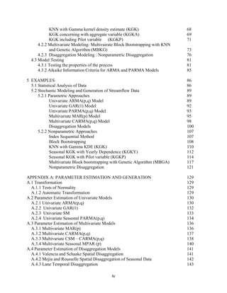
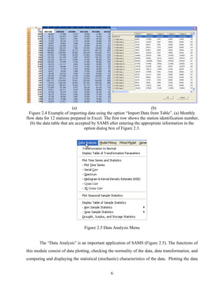
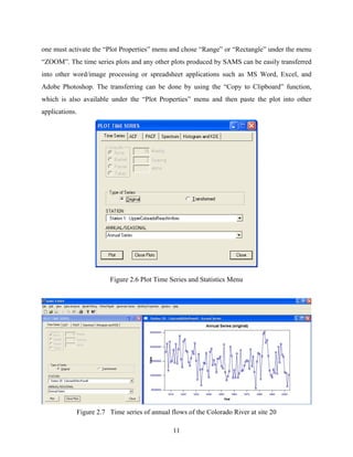
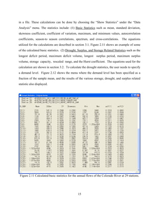
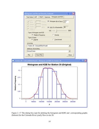
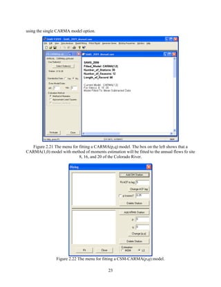
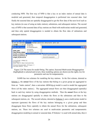
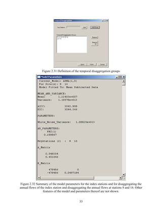
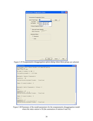
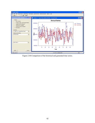
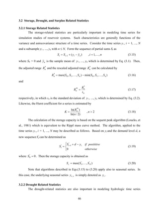
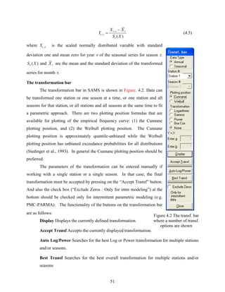
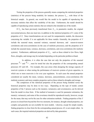
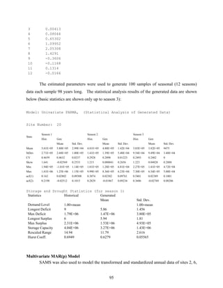
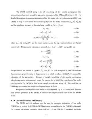
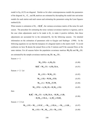
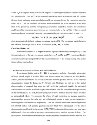
data table will appear where the number of columns is the same as the number of stations and the
number of rows is the number of years times the number of seasons (Figure 2.3). The data table
may be filled either by typing or copying and pasting from a MS Excel file table or similar
formatted table (Figure 2.4) employing [Ctrl+v] short key or paste menu in the frame. The first
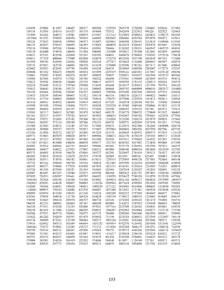
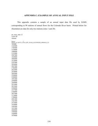
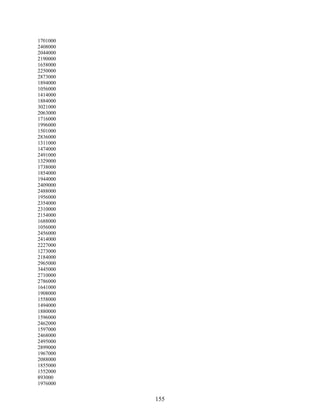
row in the table includes the site identification number and the first column beginning in row 2
gives the date of the first season and so on until the last season of the last year of record. Note
that all sites must have the same record length (with one exception, refer to section 4.1.5) and
every year must have all the seasons complete (i.e. data with values must be filled in before
entering into SAMS).
During the modeling procedure, one may want to insert one or more stations. In this case,
one can add the data of the additional stations using “Inserting data (Adding Station)”. The
procedure is the same as for ‘Importing Data from Table (e.g. excel)’ above.
Figure 2.1 The software SAMS main window menu.](https://image.slidesharecdn.com/manualdesams2009-130912131954-phpapp01/85/Manual-de-sams-2009-10-320.jpg)


![53
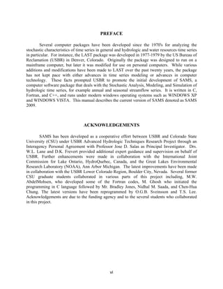
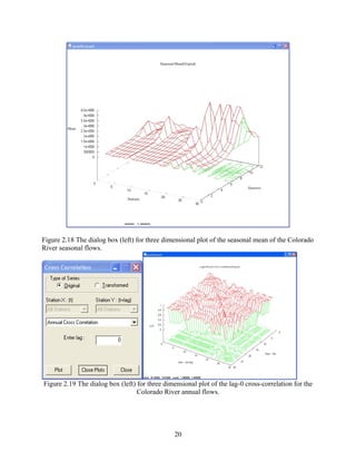
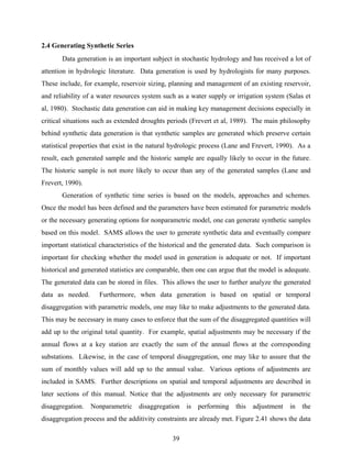
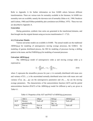
Two methods are available for estimation of the model parameters, namely the method of
moments (MOM) and the least squares method (LS). These two estimation methods are
described in Appendix A.
Univariate GAR(1)
The gamma-autoregressive model GAR(1) is similar to the well known AR(1) model
except that the underlying process being modeled is assumed to follow the gamma distribution
instead of the normal distribution. Thus if the intent is to use the GAR(1) model, then the
underlying data should not be transformed to normal by SAMS. The GAR(1) model can be
expressed as (Lawrence and Lewis, 1981)
ttt XX εφ += −1 (4.7)
where Xt is a gamma variable defined at time t, φ is the autoregression coefficient, and εt is the
independent noise term. Xt is a three-parameter gamma distributed variable with marginal density
function given by:
[ ]
)(
)(exp)(
)(
1
β
λαλα ββ
Γ
−−−
=
−
xx
xfX (4.8)
where λ, α, and β are the location, scale, and shape parameters, respectively. Lawrence (1982)
found that the independent noise term, εt, can be obtained by the following scheme:
0
00
,)1(
1
>
=
⎪⎩
⎪
⎨
⎧
=
=
+−=
∑ =
M
M
if
if
Y
where jUM
j j φη
η
ηφλε (4.9)
where M is an integer random variable distributed as Poisson with mean [- β ln(φ)], Uj , j =1,2,....
are independent identically distributed (iid) random variables with uniform (0,1) distribution,
and, Yj ,j =1,2, ....are iid random variables distributed as exponential with mean (1/α). The
stationary GAR(1) process of Eq. (4.7) has four parameters, namely {φ, λ, α, β}. The model
parameters are estimated based on a procedure suggested by Fernandez and Salas (1990), as
illustrated in Appendix A.
Univariate SM
The shifting mean (SM) model is characterized by sudden shifts or jumps in the mean.
More precisely, the underlying process is assumed to be characterized by multiple stationary
states, which only differ from each other by having different means that vary around the long
term mean of the process. The process is autocorrelated, where the autocorrelation arises only](https://image.slidesharecdn.com/manualdesams2009-130912131954-phpapp01/85/Manual-de-sams-2009-59-320.jpg)
![54
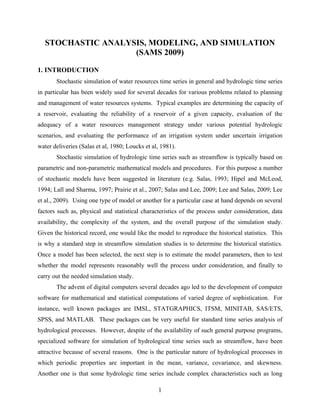
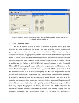
from the sudden shifting pattern in the mean. A general definition of the SM model is given by
(Sveinsson et al., 2003 and 2005)
ttt ZYX += (4.10)
where {Xt} is a sequence of random variables representing the hydrologic process of interest;
{Yt} is a sequence of iid random variables normally distributed with mean Yμ and variance 2
Yσ ;
and {Zt} is a sequence with mean zero and variance 2
Zσ . The sequences {Yt} and {Zt} are
assumed to be mutually independent of each other. The Xt process is characterized by multiple
“stationary” states each of random length Ni, i = 1,2,... as shown in Figure. 4.3. The Zt process
represents the shifting pattern from one state to another, and the different states are referred to as
noise levels. The noise level process { }tZ can be written as
( ]∑
=
−
=
t
i
SSit tIMZ ii
1
, )(1
(4.11)
Where { } ( )22
1 ,0N~ ZMii iidM σσ =∞
= , ii NNNS +++= L21 with 00 =S , and )(),( tI ba is the
indicator function equal to one if ),( bat ∈ and zero otherwise. The { }∞
=1itN is a discrete,
stationary, delayed-renewal sequence on the positive integers, with
{ } )(GeometricPositive~1 piidN it
∞
= (Sveinsson et al., 2003 and 2005). Thus the average length
of each state of the process is the inverse of the parameter of the positive Geometric distribution
or 1/p. The estimation of model parameters is described in Appendix A.
Univariate Seasonal PARMA(p,q)
Stationary ARMA models have been widely applied in stochastic hydrology for modeling
of annual time series where the mean, variance, and the correlation structure do not depend on
time. For seasonal hydrologic time series, such as monthly series, seasonal statistics such as the
mean and standard deviation may be reproduced by a stationary ARMA model by means of
standardizing the underlying seasonal series. However, this procedure assumes that season-to-
season correlations are the same for a given lag. Hydrologic time series, such as monthly
streamflows, are usually characterized by different dependence structure (month-to-month
correlations) depending on the season (e.g. spring or fall). Periodic ARMA (PARMA) models
have been suggested in the literature for modeling such periodic dependence structure. A
PARMA(p,q) model may be expressed as (Salas, 1993):](https://image.slidesharecdn.com/manualdesams2009-130912131954-phpapp01/85/Manual-de-sams-2009-60-320.jpg)
![56
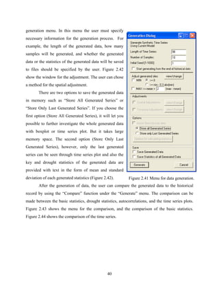
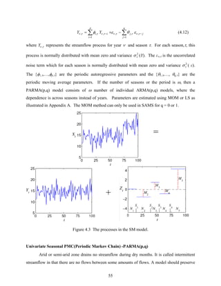
this intermittency in generation. To do this, product modeling is used assuming that τν ,Y denotes
the intermittent monthly streamflow process defined for year ν and month τ and the intermittent
variable τν ,Y is represented as the product of
τντντν ,,, ZXY ⋅=
where τν ,X is a binary (0, 1) process and τν ,Z is the amount process. The variable τν ,X defines the
occurrence of the streamflow process, i.e. 0, >τνY if 1, =τνX and 0, =τνY if 0, =τνX . Periodic
Markov Chain (PMC) model is applied for the binary process τν ,X while PARMA model is used
to model the amount process τν ,Z . The PARMA modeling is already explained in previous
chapter. Here, the PMC is described. In Markov chain modeling, it only requires the transition
matrix such that
where, 1,0,];|[),( 1,, ==== − jiiXjXPjip τντντ . The elements of the transition matrix can be
estimated with the number of data with the same states meaning that
where ),( jinτ is the number of times that the variable τν ,X being in state i at time τ-1 passes to
state j in the period τ, and )1,()0,()( ininin τττ += is the number times that τν ,X is in state i at time
τ. This PMC process is equivalent to Periodic Descrete AR(1) (PDAR(1)) model. The parameters
for PMC also are reformatted for PDRAR(1) model.
4.1.3 Multivariate Models
Analysis and modeling of multiple time series is often needed in Hydrology. In SAMS
full multivariate model are available for modeling complex dependence structure in space and
time at multiple lags. Also in SAMS, contemporaneous models are available for preserving
complex dependence structure within each site but simpler structure in space across sites.
Typical property of contemporaneous models is diagonal parameter matrixes which simplify the
parameters estimation by allowing the model to be decoupled into univariate models. The
⎥
⎦
⎤
⎢
⎣
⎡
=
)1,1()0,1(
)1,0()0,0(
ττ
ττ
pp
pp
p
)(
),(
),(ˆ
in
jin
jip
τ
τ
τ =](https://image.slidesharecdn.com/manualdesams2009-130912131954-phpapp01/85/Manual-de-sams-2009-62-320.jpg)

![66
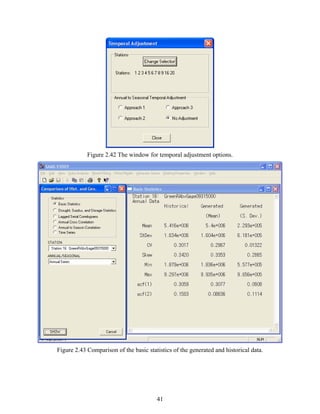
This adjustment is done for one station at a time.
approach 1:
∑
∑
=
=
−
−
−+= n
t
tt
t
t
i
q
q
qQqq
1
,
,
1
,,
)(*
,
ˆˆ
ˆˆ
)ˆˆ(ˆˆ
μ
μ
ν
ττνω
νντντν (4.32)
approach 2:
∑
=
= ω
ν
ν
τντν
1
,
,
*
,
ˆ
ˆ
ˆˆ
t
tq
Q
qq (4.33)
approach 3:
∑
∑
=
=
−+= ω
τ
ω
ντντντν
σ
σ
1
2
2
1
,,,
*
,
ˆ
ˆ
)ˆˆ(ˆˆ
t
t
t
tqQqq (4.34)
where ω is the number of seasons, νQˆ is the generated annual value, τν ,
ˆq is the generated
seasonal value, *
,
ˆ τνq is the adjusted generated seasonal value, τμˆ is the estimated mean of τν ,
ˆq for
season τ, and τσˆ is the estimated standard deviation of τν ,
ˆq for season τ.
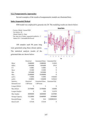
4.2 Nonparametric Approaches
4.2.1 Univariate Models
Index Sequential Method (ISM)
The index sequential method is a resampling technique that sequentially selects a block
of times series data (Ouarda et al., 1997). The method resamples the observed data with the
target length from the first observed data point and the process continues to sample the next
observed value. When the end of historic record is reached, the record is continued from the
beginning of the time series. For instance, the observed yearly time series with the record length
40 years is represented as
],...,,[ 4021 yyy=y
To resample 30 sets with 20 year length,
],,...,[)1(
~
201921 yyyy=Y , ],,...,[)2(
~
212032 yyyy=Y , ..., ],,...,[)21(
~
40392221 yyyy=Y ,
],,...,[)22(
~
1402322 yyyy=Y , …, ],,...,[)30(
~
983130 yyyy=Y](https://image.slidesharecdn.com/manualdesams2009-130912131954-phpapp01/85/Manual-de-sams-2009-72-320.jpg)
![67
where )(
~
iY is the ith
set of the resampling data.
A step size is used between the ordinal historical years used to start the various traces.
For instance a step size of three and an initial year (seed) of one would mean that the first trace
would start with the first historical year, the second trace would start with the fourth historical
year and so forth. This is done to prevent results from being biased if one wanted to only use a
limited number of traces for modeling. For seasonal data, yearly time step increment should be
used to preserve the seasonality in this method.
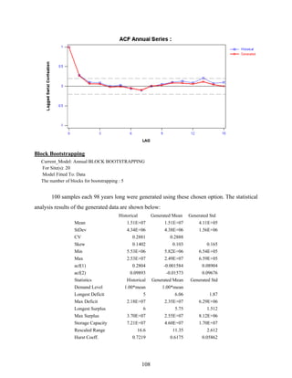
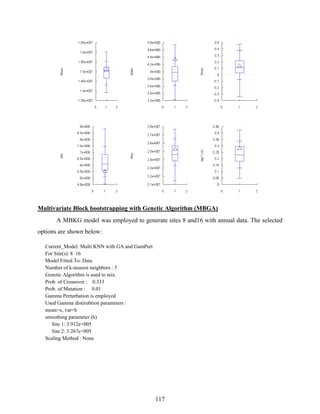
Block Bootstrapping
Block bootstrapping method is a resampling algorithm which can be used as a
nonparametric time series model (Vogel and Shallcross, 1996). The procedure is simply to
resample the historical record as a block with replacement. A block length should be long
enough to assure that the correlation structure of time series is preserved. The block can be either
overlapping or non-overlapping, that is, next block starts with the second value of the previous
block. Here, we use the overlapping blocks to have more diverse blocks.
As an example with yearly observations ],...,,[ 21 Nyyy=y , block bootstrapping is
described as follows.
(1) Set a block length l. The candidate overlapping blocks are ],...,,[ 211 lB yyy=Y ,
],...,,[ 1322 += lB yyyY , …, ],...,,[ 211 NlNlNB yyylN +−+−=+−
Y where iBY is the set of ith
block
values.
(2) One of N-l+1 blocks is selected with generating from discrete uniform random number
from 1 to N-l+1. If c is chosen from the random number, ],...,,[]
~
,...,
~
,
~
[ 1121 −++= lcccl yyyYYY
where jY
~
is the jth generated value. The block is assigned as the resampled data.
(3) The resampling of the next l values ]
~
,...,
~
,
~
[ 221 lll YYY ++ is obtained with the same procedure
as step (2). This steps are continued until the generation length is met.
For seasonal time series data, the block length should be a multiple of the total number of
seasons to preserve the seasonality of the time series.
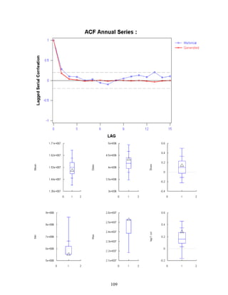
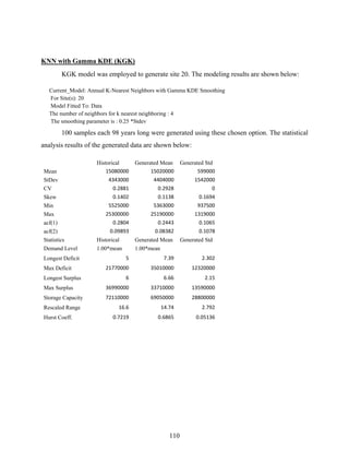
K-nearest neighbors (KNN)
The KNNR method was developed by Lall and Sharma (1996) for the generation of
yearly and monthly time series and applied to streamflow generation of the Weber River in Utah.](https://image.slidesharecdn.com/manualdesams2009-130912131954-phpapp01/85/Manual-de-sams-2009-73-320.jpg)
![70
(KGKA) is described in this section and the KGKP is followed after this section.
The conditional term (Ψ) for interannual variability is the moving aggregate flow variable
denoted as
∑
=
−=
ω
τντν
1
,,
j
jxz (4.38)
in which if 0≤− jτ , then jx −τν , becomes jx −−− των ,1 . The term τν ,z represents the sum of the
previous ω seasons. Since the generated value G
x τν , will be found by conditioning on G
x 1, −τν and
τν ,z , it is necessary to determine the weighted Euclidean distance between the generated and
historical sx′ of the previous time 1−τ and between the generated and historical sums sz′ of the
previous ω seasons. Thus the weighted distance denoted by ),( τνtr is given by
{ } 2/12
,,1
2
,1,1),( ])[(][)( HG
t
HHG
t
H
t zzzwxxxwr τντωνωωτν −+−= −− for 1,1,1 >>= tντ (4.39a)
and
{ } 2/12
,,
2
1,1,1),( ])[(][)( HG
t
HHG
t
H
t zzzwxxxwr τντττντττν −+−= −−− for 1,1 >> ντ (4.39b)
Note that the calculations of r begins at t=2 and 1=τ . The scaling weights )(1
H
xw −τ and
)( H
zwτ are the inverse of the variances of H
x 1, −τν and H
z τν , , respectively.
The procedure for simulating data based on KGKA is:
(1) Estimate the smoothing parameters k and h as suggested above, i.e. use 2/Nk = and
Eq.(4.37) to find h for each season. Then obtain the weights kiwi .,..,1, = from Eq.(4.35)
and the accumulated weights jj wwaw ++= ....1 , kj ,...,1= where 1=kaw .
(2) The initial value G
x 1,1 is randomly selected from the historical data set H
x 1,ν , ν =1,…,N. Each
historical data has an equal chance to be selected.
(3) To generate the second value G
x 2,1 obtain the absolute distances between G
x 1,1 and H
x 1,ν , i.e.
HG
xx 1,1,1 νν −=Δ , ν =1, . . ., N and order them from the smallest to the largest distance. Then
select the k smallest distances, where the smallest distance gets the largest weight and
successively up to the largest distance that gets the smallest weight. The potential values that
G
x 2,1 may take on are those k values of H
x 2,ν that correspond to the k smallest distances. Then](https://image.slidesharecdn.com/manualdesams2009-130912131954-phpapp01/85/Manual-de-sams-2009-76-320.jpg)
![72
model in such a way that not only the successive values are related but also the annual values.
For this purpose we generate a “pilot” annual data using any parametric (e.g. ARMA or shifting
mean) or nonparametric model so that the annual historical properties are preserved. The role of
the pilot variable denoted as tx′ is to serve as a surrogate of the actual annual variable, i.e. it will
be useful as an added condition in the KNNR model. The concept is that if the pilot variable tx′
say takes a small value in year t (e.g. during a drought) then it will influence the seasonal values
of that year making them also small. For this purpose we define the weighted distance ),( ttr ν as
[ ] 1)()(
2/12
2
2
,1,11),( =−′+−= −− τνωνωτν forxxwxxwr H
t
HG
tt (4.40a)
[ ] 1)()(
2/12
2
2
1,1,1),( >−′+−= −− τντνττν forxxwxxwr H
t
HG
tt (4.40b)
where 1w is the inverse of the variance of H
x 1, −τν (note that for 1=τ , 1w is the inverse of the
variance of H
x ων , ) and 2w is the inverse of the variance of the historical yearly data H
xν .
The procedure for simulating data based on KGKP is:
(1) Estimate the smoothing parameters: 2/Nk = and h (for each season) by Eq.(4.37).
(2) Generate the yearly data for the pilot variable 'tx , t=1, . . ., NG
where NG
=generation length
using any parametric or nonparametric model such as ARMA, Shifting Mean, KNNR, and
KGK. The annual historical data or an exogenous variable may be employed for this purpose.
(3) The initial value G
x 1,1 is randomly selected from the historical data set H
x 1,ν , ν =1,…,N. Each
historical data has an equal chance to be selected.
(4) To generate the second value G
tx τ, (i.e. 2,1 == τt ) get the weighted distances between G
x 1,1
and H
x 1,ν for ν =1,…,N and between the current yearly value of the pilot variable 'tx and the
historical yearly data H
xν by using Eq.(4.40a). Note that for generating G
tx τ, for 1>τ use](https://image.slidesharecdn.com/manualdesams2009-130912131954-phpapp01/85/Manual-de-sams-2009-78-320.jpg)
![74
site is equally weighted. Two kinds of scaling is applicable such as s
y
s
Y τ
μτν /, and
s
y
s
y
s
Y ττ
μστν /)( , − where s
yτ
μ and s
yτ
σ is mean and standard deviation of month τ and sth
site. In
case of intermittent process (in other words, including zero values in observations), s
yY τ
μτν /, is
preferred in order to maintain the intermittency.
From τν ,Y , a summary variable is extracted to simplify the modeling such that
∑=
=
S
s
s
Y
S
Z
1
,,
1
τντν (4.44)
From the historical data of summary variable τν ,z , a new data set can be resampled with
bootstrapping as mentioned earlier. Block bootstrapping employs the fixed block length to
preserve serial correlation. The summation of the resampled data up to yearly ∑=
=
ω
τ
τνν
1
,ZZ will be
always the same as the historical, since the block length of seasonal data should be a multiple of
total number of seasons. The main drawback of nonparametric resampling technique to employ it
as generating time series is not to reproduce any other than historical data. The simple idea to
make the block length (l) as a random variable with a certain discrete distribution will lead to
produce the unprecedented values in higher-level resampled data such as yearly. Here one of the
most common discrete distribution , Poisson distribution, is employed such that
*)!(
*)( *
l
e
lp l
λ
λ−
= (4.45)
where 1*+= ll to avoid zero value, and λ=][lE and 1*][ −= λlE . ][lE=λ is selected as the
same way of the fixed block length in the chapter of block bootstrapping.
Furthermore, even though a block is employed to preserve serial correlation structure, the
underestimation of it in the resampled data is unavoidable because there is no connectivity
between blocks. KNN is employed to solve this drawback. The first value of the next block is
selected with KNN. The distances are measured by
1,1,
~
),( −− −= ττντν ii zZd
where Ni ,..,1= . The same procedure of KNN is performed to choose τν ,
~
Z . And the next l-1
values are followed such that if ττν ,,
~
czZ = (that is, year c is selected from KNN),
],...,[]
~
,...,
~
[ 1,,1,1, −+−++ = lccl zzZZ τττντν . The detailed procedures are as follows.](https://image.slidesharecdn.com/manualdesams2009-130912131954-phpapp01/85/Manual-de-sams-2009-80-320.jpg)
![75
1. Set the parameters k (KNN) and λ (block bootstrapping)
2. Generate the block length ( 1l ) from the Poisson distribution in Eq.(4.45).
3. Select a block with 1l starting from the month 1. Discrete uniform random number from
zero to the record length N is used to select the initiating value. Assume that 1c is chosen
from the discrete random number. Then ],...,,[]
~
,...,
~
[ 11111 ,2,1,,11,1 lcccl zzzZZ = . Here, if ω>1l ,
ω−+= 11 ,1, lili zz . The multivariate original data τν ,
~
Y is assigned with the corresponding τν ,
~
Z .
For example, if 1,1,1 1
~
czZ = , where ∑=
=
S
s
s
cc yz
1
1,1, 11
then
⎥
⎥
⎥
⎥
⎥
⎦
⎤
⎢
⎢
⎢
⎢
⎢
⎣
⎡
=
S
c
c
c
y
y
y
1,
2
1,
1
1,
1,1
1
1
1
~
M
Y
4. The next block length 2l is generated from the Poisson distribution. At first, the next
value 1,1 1
~
+lZ is selected with KNN with concerning the seasonality. Assuming that year 2c
is chosen, the following 2l length data are chosen such that
],...,,[]
~
,...,
~
[ 2111112211 ,2,1,,11,1 llclclclll zzzZZ +++++ = and assign ]
~
,...,
~
[ 211 ,1, lll ++ νν YY according to τν ,
~
Z .
5. The procedure 4 is repeated until the generation length is met.Since the summary variable
is used to generate time series, the output sequences will be always the same as the
historical between sites. For example, if τ,cz is selected, then
[ ]TS
ccc yyy ττττν ,
2
,
1
,, 1021
,...,,
~
=Y where 1021 ... cccc ==== and superscript T means the
transpose of a vector. The property that 1021 ... cccc ==== is not desirable because it
implies that there is no variability between resampled sites. We use Genetic Algorithm to
mingle the sequence so that the property can be broken while preserving cross-
correlation. Genetic algorithm has been employed to find approximate or exact solutions
with biologic elocutionary system. The parallel traveling power to produce the best
solution is employed here for nonparametric time series simulation modeling. The
generation procedure of MGBG is explained for seasonal case as follows.
Genetic Algorithm Procedure for seasonal data
During the steps 3 and 4 of the procedure above, one more multivariate data set τν ,*
~
Y is](https://image.slidesharecdn.com/manualdesams2009-130912131954-phpapp01/85/Manual-de-sams-2009-81-320.jpg)
![76
selected with KNN close to τν ,
~
Z . The distances are measured as ττν ,,
~
ii zZd −= where
Ni ,...,1= . Among the smallest id s, one is selected from the discrete weighted distribution as in
Eq.(3), say )2(cd . The corresponding value τ),2(cz and its original data set is taken, say
ττν ),2(,*
~
cyY = . The present generated value TS
YY ]
~
,...,
~
[
~
,
1
,, τντντν =Y are replaced with
TS
YY *]
~
*,...,
~
[*
~
,
1
,, τντντν =Y or kept as it is element-by-element with the crossover probability such
that if
⎪⎩
⎪
⎨
⎧ <
=
otherwise
~
*
~
~
,
,
, s
c
s
s
Y
upY
Y
τν
τν
τν
where s=1,…,S, cp is the crossover probability and its default is 0.333 as suggested in Goldberg
(1998), and u is the uniform random number from zero to one. In case that s
Y τν ,
~
stays as it is,
mutation process is performed such that
⎪⎩
⎪
⎨
⎧ <
=
otherwise
~
~
,
,
, s
m
s
cs
Y
upy
Y
m
τν
τ
τν
where s
cm
y τ, is the selected observation and mc is selected with the discrete uniform distribution
from one to N.
Furthermore, if the new value other than the observations is desired, Gamma perturbation
can be used. Two way of perturbations are in the option. The first one is the same as of KGK as
in Eq.(4.36). The second one is
)()/
~
(
)(
)/
~
/(1
/
~
,
hhY
et
tK h
hYth
hYh
Γ
=
−−
where Y
~
is the resampled data. The latter is used when data are highly skewed. The mean and
variance from the gamma kernel are xt =)(μ and hxt /)( 22
=σ respectively. The smoothing
parameter is
222
/)(4/ xxxNh σμσ +⋅= . The detailed description is referred to Lee and Salas 2008.
4.2.3 Disaggregation Modeling : Nonparametric Disaggregation
The implemented nonparametric disaggregation (NPD) model in SAMS2009 is the combined](https://image.slidesharecdn.com/manualdesams2009-130912131954-phpapp01/85/Manual-de-sams-2009-82-320.jpg)


![126
REFERENCES
Boswell, M.T., Ord, J.K., and Patil, G.P., 1979. Normal and lognormal distributions as models
of size. Statistical Distributions in Ecological Work, J.K. Ord, G.P. Patil and C.Taillie
(editors), 72-87, Fairland, MD: International Cooperative Publishing House.
Brockwell, P.J. and Davis, R.A., 1996. Introduction to Time Series and Forecasting. Springer
Texts in Statistics. Springer-Verlag, first edition.
Chen, S. X. ,2000, Probability density function estimation using gamma kernels, Annals of the
Institute of Statistical Mathematics, 52, 471-480
Fernandez, B., and J.D. Salas, 1990, Gamma-Autoregressive Models for Stream-Flow
Simulation, ASCE Journal of Hydraulic Engineering, vol. 116, no. 11, pp. 1403-1414.
Filliben, J.J., 1975. The probability plot correlation coefficient test for normality. Technometrics,
17(1):111–117.
Frevert, D.K., M.S. Cowan, and W.L. Lane, 1989, Use of Stochastic Hydrology in Reservoir
Operation, J. Irrig. Drain. Eng., 115(3), pp. 334-343.
Gill, P E., W. Murray, and M.H. Wright, 1981, Practical Optimization, Academic Press, N.
York.
Goldberg, D. E. (1989), Genetic algorithms in search, optimization, and machine learning,
Addison-Wesley Pub. Co.
Grygier, J.C., and Stedinger, J.R., 1990., “SPIGOT, A Synthetic Streamflow Generation
Software Package”, technical description, version 2.5, School of Civil and Environmental
Engineering, Cornell University, Ithaca, N.Y.
Himmenlblau, D.M., 1972, Applied Nonlinear Programming, McGraw-Hill, New York.
Hipel, K. and McLeod, A.I. 1994. "Time Series Modeling of Water Resources and
Environmental Systems", Elsevier, Amsterdam, 1013 pages.
Hurvich, C.M. and Tsai, C.-L., 1989. Regression and time series model selection in small
samples. Biometrika, 76(2):297–307.
Hurvich, C.M. and Tsai, C.-L., 1993. A corrected Akaike information criterion for vector
autoregressive model selection. J. Time Series Anal. 14, 271–279.
Kendall, M.G., 1963, The advanced theory of statistics, vol. 3, 2nd Ed., Charles Griffin and Co.
Ltd., London, England.
Lane, W.L., 1979, Applied Stochastic Techniques (Last Computer Package); User Manual,
Division of Planning Technical Services, U.S. Bureau of Reclamation, Denver, Colo.
Lane, W.L., 1981, Corrected Parameter Estimates for Disaggregation Schemes, Inter. Symp. On
Rainfall Runoff Modeling, Mississippi State University.
Lane, W.L., and D.K. Frevert, 1990, Applied Stochastic Techniques, personal computer version
5.2, users manual, Bureau of Reclamation, U.S. Dep. of Interior, Denver, Colorado.
Lawrance, A.J., 1982, The innovation distribution of a gamma distributed autoregressive
process, Scandinavian J. Statistics, 9(4), 234-236.
Lawrance, A.J. and P. A. W. Lewis, 1981, A New Autoregressive Time Series Model in
Exponential Variables [NEAR(1)], Adv. Appl. Prob., 13(4), pp. 826-845.
Lee and Salas (2008), Multivariate Simulation Modeling with the Combination of Intermittent
and Non-intermittent for Monthly Time Series : KNN Match Moving block bootstrapping
with Genetic Algorithm and Perturbation Gamma KDE
Lee, T. and Salas, J.D., 2009. Multivariate Simulation Monthly Streamflows of Intermittent and
Non-intermittent.
Lee, T., Salas, J.D. and Prarie, J., 2009. Nonparametric Streamflow Disaggregation Model in
review.](https://image.slidesharecdn.com/manualdesams2009-130912131954-phpapp01/85/Manual-de-sams-2009-132-320.jpg)
![131
111
11
11
ˆ
1
ˆ
ˆ1ˆˆ
θφ
φ
φθ −
−
−
+=
r
r
(A.6)
1
1122
ˆ
ˆ
)(ˆ
θ
φ
εσ
r
s
−
= (A.7)
where 1
ˆθ is estimated by solving Eq. (A.6).
- ARMA (2,1) model:
112211 −−− −++= ttttt YYY εθεφφ (A.8)
2
2
1
312
1
ˆ
rr
rrr
−
−
=φ (A.9)
1
213
2
ˆ
ˆ
r
rr φ
φ
−
= (A.10)
11211
1211
1211
2211
11
ˆ)ˆˆ(
ˆˆ
ˆˆ
ˆˆ1ˆˆ
θφφ
φφ
φφ
φφ
φθ
rr
rr
rr
rr
+−
+−
−
+−
−−
+= (A.11)
1
112122
ˆ
ˆˆ
)(ˆ
θ
φφ
εσ
rr
s
−+
= (A.12)
where s2
is the variance of Yt and rk = mk / s2
is the estimate of the lag-k autocorrelation
coefficient of Yt which is defined as Rk = E[Yt Yt-k] / E[Yt Yt]. Similarly mk is the estimate of the
lag-k autocovariance coefficient of Yt with Mk = E[Yt Yt-k]. In the foregoing model it is assumed
that the mean has been removed or E[Yt] = 0. Note also that s2
= m0.
The Least Squares (LS) method is generally a more efficient parameter estimation
method. In this method, the parameters φ’s and θ’s are estimated by minimizing the sum of
squares of the residuals defined by
∑
=
=
N
t
tF
1
2
ε (A.13)
where N is the number of years of data. For the ARMA(p,q) model, the residuals are defined as
∑∑
=
−
=
− +−=
q
j
jtj
p
i
ititt YY
11
εθφε (A.14)
Once the φ’s and θ’s are determined, then the noise variance σ2
(ε) is determined by
∑=
N
t tN 1
2
)/1( ε . The minimization of the sum of squares of Eq. (A.13) may be obtained by a
numerical scheme. In SAMS first a high order AR(p) model is fitted to the data to get initial](https://image.slidesharecdn.com/manualdesams2009-130912131954-phpapp01/85/Manual-de-sams-2009-137-320.jpg)
![135
below (Salas et al, 1982):
- PARMA (1,1) model:
1,,1,1,,1, −− −+= τνττντνττν εθεφ YY (A.35)
1,1
,2
,1
ˆ
−
=
τ
τ
τφ
m
m
(A.36)
1,1,1
2
1,1
1,1
2
1,1
,1
2
1,1
,1,1
2
,1,1
ˆ)ˆ(
ˆ
ˆ
ˆ
ˆˆ
+−
++
− −
−
−
−
−
+=
ττττ
τττ
τττ
τττ
ττ
θφ
φ
φ
φ
φθ
ms
ms
ms
ms
(A.37)
1,1
1,1
2
11,12
ˆ
ˆ
)(ˆ
+
+−+ −
=
τ
τττ
τ
θ
φ
εσ
ms
(A.38)
- PARMA (2,1) model:
1,,1,2,,21,,1, −−− −++= τνττντνττνττν εθεφφ YYY (A.39)
1,2
2
22,11,1
,3
2
22,1,2
,1
ˆ
−−−−
−−
−
−
=
ττττ
ττττ
τφ
msmm
msmm
(A.40)
2,1
1,2,1,3
,2
ˆ
ˆ
−
−−
=
τ
τττ
τ
φ
φ
m
mm
(A.41)
1,11,1,2,1
2
1,1
,11,21,1
2
1,1
1,1,2,1
2
1,1
,2,2,1,1
2
,1,1 ˆ)ˆˆ(
ˆˆ
ˆˆ
ˆˆ
ˆˆ
+−−
+++
−− +−
+−
−
+−
−−
+=
ττττττ
τττττ
τττττ
τττττ
ττ
θφφ
φφ
φφ
φφ
φθ
mms
mms
mms
mms
(A.42)
1,1
1,1,11,2
2
1,12
ˆ
ˆˆ
)(ˆ
+
+++ −+
=
τ
τττττ
τ
θ
φφ
εσ
mms
(A.43)
wheres 2
τs is the seasonal variance and τ,km is the estimate of the lag-k season-to-season
autocovariance coefficient of τν ,Y which is defined as Mk,τ = E[Yν,τ Yν,τ-k], where it is assumed
E[Yν,τ] = 0. Note also that ττ ,0
2
ms = .
In a similar manner as for the ARMA(p,q) model, the Least Squares (LS) method can be
used to estimate the model parameters of PARMA(p,q) models. In this case, the parameters φ’s
and θ’s are estimated by minimizing the sum of squares of the residuals defined by
∑∑
= =
=
N
F
1 1
2
,
ν
ω
τ
τνε (A.44)](https://image.slidesharecdn.com/manualdesams2009-130912131954-phpapp01/85/Manual-de-sams-2009-141-320.jpg)
![136
where ω is the number of seasons and N is the number of years of data. For the PARMA(p,q)
model, the residuals are defined as
∑∑
=
−
=
− +−=
q
j
jj
p
i
ii YY
1
,,
1
,,,, τνττνττντν εθφε (A.45)
Once the φ’s and θ’s are determined the seasonal noise variance )(2
εστ can be estimated by
∑ =
N
N 1
2
,)/1( ν τνε .
Generation of data from PARMA(p,q) models is carried out in a similar manner as for
ARMA(p,q) models. The warm up length procedure is used to generate seasonal sequences of
the τν ,Y process by assuming that values of τν ,Y prior to season 1 of year 1 are equal to zero and
generating uncorrelated random sequences of τνε , as needed in a similar manner as for the
ARMA (p,q) model. The warm-up period is taken as 50 years.
A.3 Parameter Estimation of Multivariate Models
A.3.1 Multivariate MAR(p)
The MOM method is used for parameter estimation of the MAR(p) model. It can be
shown that the MOM equations of the MAR(p) model in Eq. (4.13) are given by:
∑
=
Φ+=
p
i
T
ii
1
0 MGM (A.46)
∑
=
− ≥Φ=
p
i
ikik k
1
1,MM (A.47)
where Mk is the lag-k cross covariance matrix of Yt defined as:
][ T
kttk E −= YYM (A.48)
in which the superscript T indicates a matrix transpose and E[Yt] = 0. In finding the MOM
estimates, Eq. (A.47) for k = 1, ..., p, is solved simultaneously for the parameter matrixes iΦ , i =
1,..., p, by substituting in Eq. (A.47) the population covariance matrixes Mk , k = 1,2,..., p, by the
sample covariance matrixes mk, k = 1,2,..., p. Then Eq. (A.46) is used to estimate the variance-
covariance matrix of the residuals G . For example, the moment estimators of the MAR(1)
model are:
0
1
1
ˆ
m
m
=Φ (A.49)](https://image.slidesharecdn.com/manualdesams2009-130912131954-phpapp01/85/Manual-de-sams-2009-142-320.jpg)
![137
T
1
1
010
ˆ mmmmG −
−= (A.50)
in which superscript -1 indicates a matrix inverse.
After estimating iΦ , i = 1,..., p, and G as indicated above, B of Eq. (4.14) can be
determined from
T
BBG ˆˆˆ = (A.50)
The above matrix equation can have more than one solution. However, a unique solution can be
obtained by assuming that B is a lower triangular matrix. This solution, however, requires that G
be a positive definite matrix.
Generation of synthetic series for the MAR(p) model is carried out using Eq. (4.13) with
the spatially correlated noise generated by Eq. (4.14). The warm-up period is defined in the
same way as for the ARMA model.
A.3.2 Multivariate CARMA(p,q)
The parameter matrixes of the CARMA(p,q) in Eq. (4.15) are diagonal. Thus, as
described in section 4.3.2 the estimation of parameters of the CARMA model is done by
decoupling it into univariate ARMA models:
∑∑
=
−
=
− −+=
q
j
k
jt
k
j
k
t
p
i
k
it
k
i
k
t YY
1
)()()(
1
)()()(
εθεφ (A.51)
where the superscript (k) indicates the kth site and as such the parameters shown indicate the kk
diagonal element in the diagonal parameter matrixes in Eq. (4.15). The best univariate ARMA
model is identified for each site and the parameters are estimated at each site using MOM or LS
estimation methods. After having estimated the diagonal parameter matrixes pΦΦΦ ,,, 21 K
and qΘΘΘ ,,, 21 K , what remains is estimation of the noise variance-covariance matrix G. The
procedure is simple, but a necessary condition is that the CARMA(p,q) is causal. This is
equivalent to requiring each of the estimated univariate ARMA(p,q) models to be causal (often a
common requirement in estimation procedures for ARMA models). Causality implies that Yt in
Eq. (4,15) can be written out as an infinite moving average model (Brockwell and Davis, 1996):
∑
∞
=
−Ψ=
0j
jtjt εY (A.52)
where E[Yt] = 0 and jΨ are matrixes with absolutely summable elements given by](https://image.slidesharecdn.com/manualdesams2009-130912131954-phpapp01/85/Manual-de-sams-2009-143-320.jpg)
![141
∑
=
−− ≥≥−Φ=
p
i
iikik kandifor
1
,,, 10, ττττ MM (A.60a)
∑
=
−− ≥<−Φ=
p
i
T
kkiik kandifor
1
,,, 10, ττττ MM (A.60b)
where Mk,τ is the lag-k cross covariance matrix of Yν,τ defined as:
T
kk
T
k
T
kk EE −−−− === ττντντντντ ,
T
,,,,, ]}[{][ MYYYYM (A.62)
in which the superscript T indicates a matrix transpose and E[Yν,τ] = 0. In a similar manner as
for the MAR(p) model, the MOM estimates can be found by solving Eq. (A.60) for k =1,2,..., p
simultaneously for Φ ’s by substituting the population covariance matrixes τ,kM , k = 1,…,p by
the corresponding sample covariance matrixes. Then Eq. (A.59) is used to estimate the variance-
covariance matrix of the residuals τG .
For generation of synthetic time series similar procedures as for the MAR(p) and
PARMA(p,q) models are used. As for the MAR(p) model the generation process of the noise is
simplified by using a lower triangular matrix τB similar as in Eq. (4.14) for the MAR(p) model,
i.e. T
τττ BBG = . As for other models a warm-up period is used to remove the effects of initial
conditions of the generation process.
A.4 Parameter Estimation of Disaggregation Models
A.4.1 Valencia and Schaake Spatial Disaggregation
The model parameter matrixes A and B of the VS model in Eq. (4.18) can be estimated
by using MOM (Valencia and Schaake, 1973):
)()( 1
00 XMYXMA −
= (A.63)
1
00 )()( −
−= AXMAYMBBT
(A.64)
where T
BBG = is the noise variance-covariance matrix (B is the Cholesky decomposition of
G), and ][)( T
kk E −= νν YYYM and ][)( T
kk E −= νν XYYXM . The VS model is not available for
spatial disaggregation of seasonal data in SAMS, since the MR model is thought to be better
suited.
A.4.2 Mejia and Rousselle Spatial Disaggregation
The model parameter matrixes A, B, and C of the MR model in Eq. (4.19) can be
estimated by using MOM as:
-1
1
1
0101
1
010 ])()()()(][)()()()([ XYMYMXYMXMXYMYMYMYXMA TT −−
−−= (A.65)](https://image.slidesharecdn.com/manualdesams2009-130912131954-phpapp01/85/Manual-de-sams-2009-147-320.jpg)
![142
)(])()([ 1
011 YMXYAMYMC −
−= (A.66)
)()()( 100 YCMXYMAYMBB TT
−−= (A.67)
Equations (A.65) through (A.67) can be used to obtain estimates of A, B, and C by substituting
the population covariance matrixes by their corresponding sample estimates. Lane (1981)
showed that some problems exist if one uses the above equations to estimate the parameters.
Specifically, the problem is in using )(1 XYM , since the model structure does not preserve this
particular lag-1 dependence between X and Y. Lane verified this and showed that the generated
moments are affected and some key moments are not preserved. As a result, he suggested that,
instead of using a sample estimate of )(1 XYM , one should use the model )(1 XYM that would
result from the model structure (for further details, the reader is referred to Lane and Frevert,
1990). In the final analysis, the suggested equation is
)()()()( 0
1
01
*
1 XYMXMXMXYM −
= (A.68)
For consistency )(1 YM also needs to be adjusted
])()([)()()()( 1
*
1
1
001
*
1 XYMXYMXMYXMYMYM −+= −
(A.69)
Equations (A.68) and (A.69) should be used for calculating )(1 XYM and )(1 YM , and these
calculated values should be used in Eqs. (A.65) through (A.67) for estimating the model
parameters. The reader is referred to Lane and Frevert (1990) for more in depth details about
these adjustments.
A.4.2 Mejia and Rousselle Spatial Disaggregation of Seasonal Data
The model parameter matrixes τA , τB , and τC of the MR model in Eq. (4.21) can be
estimated in a similar way as for the spatial disaggregation of annual data above by using MOM.
The MOM equations are similar as for the annual MR model:
1-
,1
1
1,0,1,0
,1
1
1,0,1,0
])()()()([
])()()()([
XYMYMXYMXM
XYMYMYMYXMA
T
T
ττττ
τττττ
−
−
−
−
−
−=
(A.70)
)(])()([ 1
1,0,1,1 YMXYMAYMC −
−−= τττττ (A.71)
)()()( ,1,0,0 YMCXYMAYMBB TT
τττττττ −−= (A.72)
where ][)( ,,,
T
kk E −= τντντ YYYM and ][)( ,,,
T
kk E −= τντντ XYYXM . Since the model structure of
Eq. (4.21) does not preserve the dependence structure between τν ,X and 1, −τνY for any season,](https://image.slidesharecdn.com/manualdesams2009-130912131954-phpapp01/85/Manual-de-sams-2009-148-320.jpg)
![143
same type of adjustment procedures as for the annual MR model have to be applied for each
season for estimation of )(,1 YM τ and )(,1 XYM τ . Thus for each season the following corrected
model covariances are used:
)()()()( 1,0
1
1,0,1
*
,1 XYMXMXMXYM −
−
−= ττττ (A.73)
])()([)()()()( ,1
*
,1
1
,0,0,1
*
,1 XYMXYMXMYXMYMYM ττττττ −+= −
(A.74)
The above corrected model covariances need to be substituted into the MOM equations, and then
the estimates of A, B, and C are obtained by substituting the population covariance matrixes in
the MOM equations by their corresponding sample estimates.
A.4.3 Lane Temporal Disaggregation
The model parameter matrixes τA , τB , and τC of the temporal Lane model in Eq. (4.22)
can be estimated by using the MOM as (Lane and Frevert, 1990). To avoid confusion we have X
denote the annual flows at the N stations and Y the seasonal flows at the same stations.
1-
,1
1
1,0,10
,1
1
1,0,1,0
])()()()([
])()()()([
XYMYMXYMXM
XYMYMYMYXMA
T
T
τττ
τττττ
−
−
−
−
−
−=
(A.75)
)(])()([ 1
1,0,1,1 YMXYMAYMC −
−−= τττττ (A.76)
)()()( ,1,0,0 YMCXYMAYMBB TT
τττττττ −−= (A.77)
where ][)( T
kk E −= νν XXXM , ][)( ,,,
T
kk E −= τντντ YYYM , ][)( ,,
T
kk E −= τνντ YXXYM and
][)( ,,
T
kk E −= ντντ XYYXM . Since the model structure of Eq. (4.22) does preserve the dependence
structure between νX and 1, −τνY (i.e. )(,1 XYM τ ) for all seasons except the first one, adjustment
procedures as for the MR models need only to be applied for the first season in estimation of
)(,1 YM τ and )(,1 XYM τ . Thus only for the first season need the following corrected model
covariances to be used:
)()()()( 1,0
1
01
*
,1 XYMXMXMXYM −
−
= ττ (A.78)
])()([)()()()( ,1
*
,1
1
0,0,1
*
,1 XYMXYMXMYXMYMYM τττττ −+= −
(A.79)
The MOM parameter matrixes are then estimated by substituting the population moments by
their corresponding sample estimates.
A.4.5 Grygier and Stedinger Temporal Disaggregation
The parameter matrixes of the contemporaneous Grygier and Stedinger disaggregation](https://image.slidesharecdn.com/manualdesams2009-130912131954-phpapp01/85/Manual-de-sams-2009-149-320.jpg)


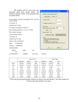
This document provides a user's manual for SAMS (Stochastic Analysis, Modeling, and Simulation) version 2009. SAMS is a software package developed by Colorado State University and the U.S. Bureau of Reclamation to analyze and model stochastic hydrologic time series, such as annual and seasonal streamflow, using parametric and nonparametric methods. The manual describes the capabilities and components of SAMS 2009, which includes data analysis tools, stochastic models for single-site and multi-site data as well as disaggregation models, and generation of synthetic hydrologic time series. Parameter estimation techniques and model testing procedures for the various stochastic models in SAMS 2009 are also outlined.


![Hec ras 4.1-applications_guide[1]](https://cdn.slidesharecdn.com/ss_thumbnails/hec-ras4-140906052124-phpapp01-thumbnail.jpg?width=640&height=640&fit=bounds)