Download to read offline


![www.robertodaguarcino.com
Features of the files were loaded into Design Matrix 𝑿 ∈ 𝑅 𝑁×𝐷
and the output in 𝒚 ∈ 𝑅 𝑁
,
𝑦𝑖 ∈ {𝑃𝑙𝑎𝑛𝑘𝑡𝑜𝑛, 𝐹𝑎𝑘𝑒𝐼𝑛𝑠𝑡𝑎𝑙𝑙𝑒𝑟, 𝑒𝑡𝑐. }:
𝑿 = [
𝑥11 ⋯ 𝑥1𝑛
⋮ ⋱ ⋮
𝑥 𝑛1 ⋯ 𝑥 𝑛𝑛
]
𝒚 = (
𝑦1
⋮
𝑦𝑛
)
4.3 From nominal data to numeric data
Nominal data (or categorical data) are variables that contain label values rather than numeric
values. The number of possible values is often limited to a fixed set. Categorical variables are
often called nominal.
Some examples include:
A “pet” variable with the values: “dog” and “cat“.
A “color” variable with the values: “red“, “green” and “blue“.
A “place” variable with the values: “first”, “second” and “third“.
Each value represents a different category.
Some categories may have a natural relationship to each other, such as a natural ordering.
The “place” variable above does have a natural ordering of values. This type of categorical
variable is called an ordinal variable.
What is the Problem with Categorical Data?
Some algorithms can work with categorical data directly.](https://image.slidesharecdn.com/malwareanalysis-190117151733/75/Malware-analysis-7-2048.jpg)

![www.robertodaguarcino.com
Making decisions means applying all classifiers to an unseen sample x and predicting the class
k for which the corresponding classifier reports the highest confidence score:
𝑦̂ = 𝑎𝑟𝑔𝑚𝑎𝑥 𝑓𝑘(𝑥), 𝑘 ∈ {1, … , 𝐾}
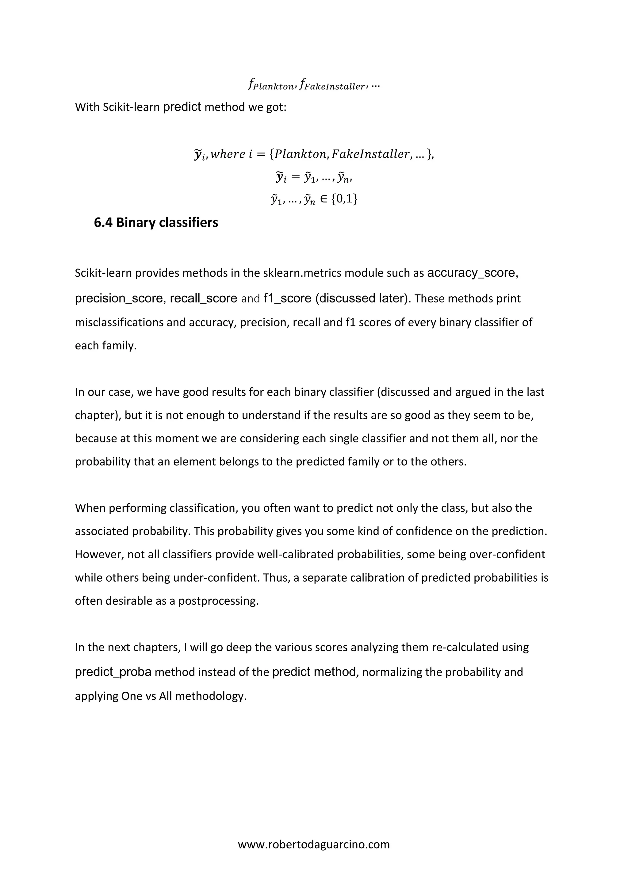
Thanks to predict_proba method of Scikit-learn we have:
𝒚̂𝑖, 𝑖 = {𝑃𝑙𝑎𝑛𝑘𝑡𝑜𝑛, 𝐹𝑎𝑘𝑒𝐼𝑛𝑠𝑡𝑎𝑙𝑙𝑒𝑟, … },
𝒚̂𝑖 = 𝑦̂1, … , 𝑦̂ 𝑛,
𝑦̂1, … , 𝑦̂ 𝑛 ∈ [0,1]
that represent this confidence score in a probability status.
To normalize the partial results (∑ 𝒚̅𝑖 𝑖
= 1):
𝒚̅𝑖, 𝑖 = {𝑃𝑙𝑎𝑛𝑘𝑡𝑜𝑛, 𝐹𝑎𝑘𝑒𝐼𝑛𝑠𝑡𝑎𝑙𝑙𝑒𝑟, … },
𝒚̅𝑖 =
𝒚̂𝑖
𝒚̂ 𝑃𝑙𝑎𝑛𝑘𝑡𝑜𝑛 + 𝒚̂ 𝐹𝑎𝑘𝑒𝐼𝑛𝑠𝑡𝑎𝑙𝑙𝑒𝑟 + ⋯
At last, we can apply the majority rule with a threshold of 0.50 confidence score:
𝐼𝑓 𝒚̅𝑖 > 0.50 ⇒ 𝒚̅𝑖 ∈ 𝑖, 𝑖 = {𝑃𝑙𝑎𝑛𝑘𝑡𝑜𝑛, 𝐹𝑎𝑘𝑒𝐼𝑛𝑠𝑡𝑎𝑙𝑙𝑒𝑟, … }
else, it goes to a misclassification.
Once proceeds the confidence score (or misclassifications) for every family, we can calculate
scores to understand if the classification can be good enough. In the next paragraphs there
will be discussed each used score and in the final chapter it will be analyzed my code’s results.
6.7 Accuracy score
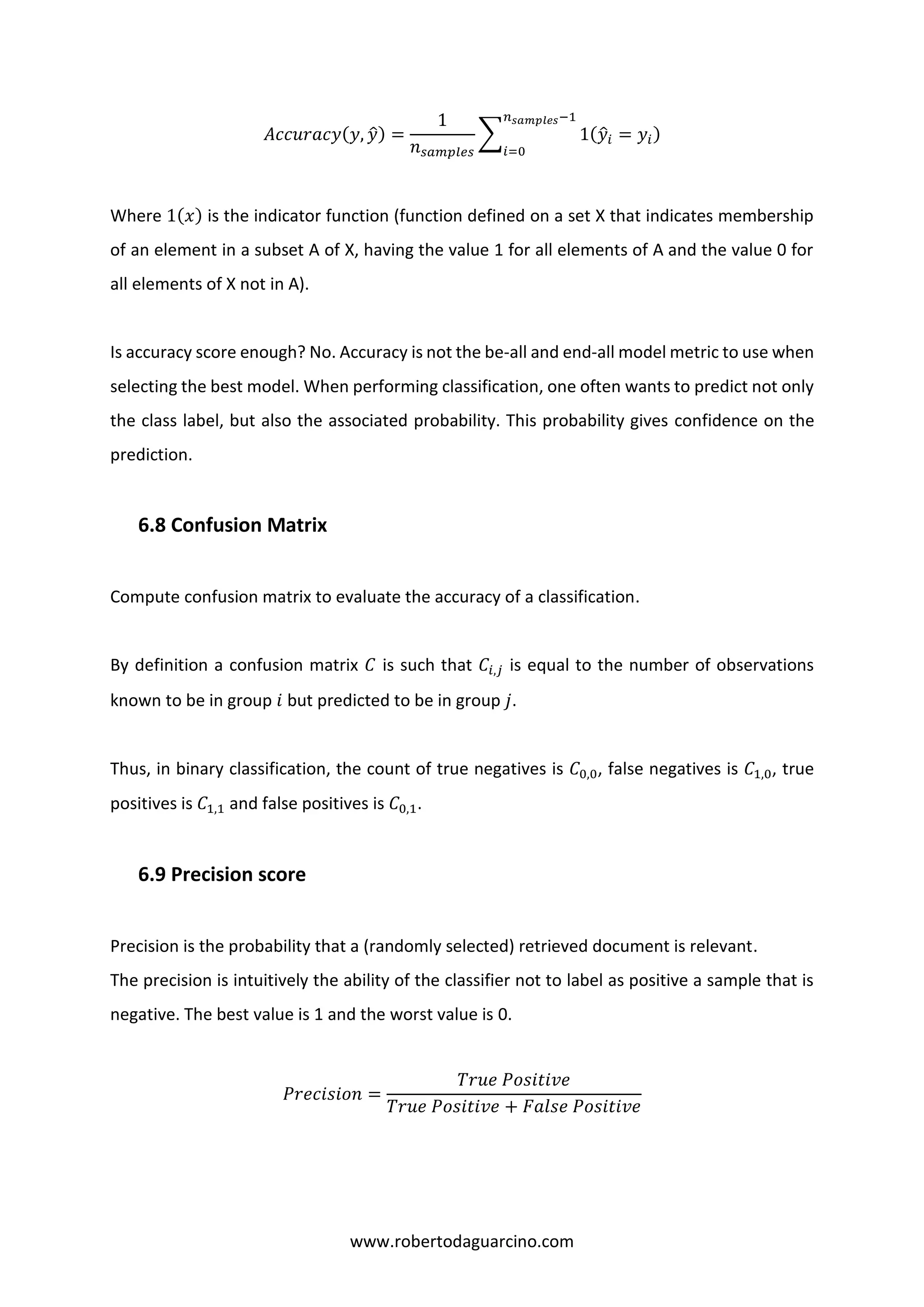
The accuracy_score function computes the accuracy, either the fraction (default) or the count
(normalize=False) of correct predictions. If 𝑦̂𝑖 is the predicted value of the 𝑖-th sample and 𝑦𝑖
is the corresponding true value, then the fraction of correct predictions over 𝑛 𝑠𝑎𝑚𝑝𝑙𝑒𝑠 is
defined as](https://image.slidesharecdn.com/malwareanalysis-190117151733/75/Malware-analysis-15-2048.jpg)
![www.robertodaguarcino.com
6.11 F1 score
F1 score, also known as balanced F-score or F-measure, can be interpreted as a weighted
average of the precision and recall, where an F1 score reaches its best value at 1 and worst
value at 0. The relative contribution of precision and recall to the F1 score are equal. In the
multi-class and multi-label case, this is the average of the F1 score of each class with weighting
depending on the average parameter.
𝐹1 = 2 ×
𝑃𝑟𝑒𝑐𝑖𝑠𝑖𝑜𝑛 ∗ 𝑅𝑒𝑐𝑎𝑙𝑙
𝑃𝑟𝑒𝑐𝑖𝑠𝑖𝑜𝑛 + 𝑅𝑒𝑐𝑎𝑙𝑙
F1 Score is needed when you want to seek a balance between Precision and Recall. We have
previously seen that accuracy can be largely contributed by a large number of True Negatives
which in most business circumstances, we do not focus on much whereas False Negative and
False Positive usually has business costs (tangible & intangible) thus F1 Score might be a better
measure to use if we need to seek a balance between Precision and Recall and there is an
uneven class distribution (large number of Actual Negatives).
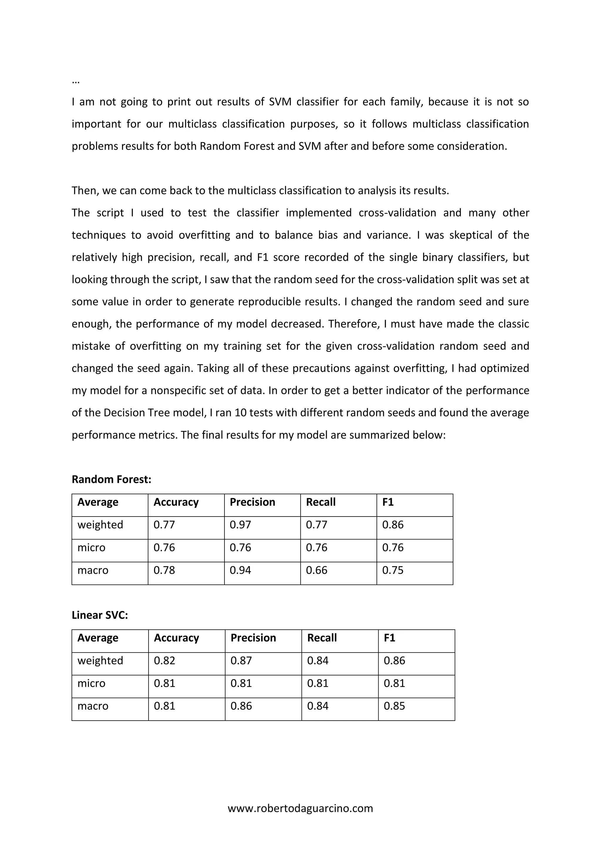
7. Final results
After reasoned and argued all my program and the procedures I followed to solve the
multiclass classification problem, I am going to write into this chapter results and
consequences of what I discovered and why.
All binary classifiers, applied on each family, have very good scores, including accuracy,
balanced accuracy, misclassification rate, recall, precision and f1.
Here are the results of some family, using a 3-fold cross validation with Random Forest.
Family #0: GinMaster
accuracy: [0.98825372 0.99451411 0.99137255]](https://image.slidesharecdn.com/malwareanalysis-190117151733/75/Malware-analysis-18-2048.jpg)
![www.robertodaguarcino.com
balanced accuracy: [0.90555556 0.97180064 0.96067416]
misclassification: 8
recall: [0.98747063 0.98981191 0.9945098 ]
precision: [0.99146515 0.99446995 0.99369643]
f1: [0.98285934 0.99449994 0.9903826 ]
Family # 1: FakeInstaller
accuracy: [0.97137931 0.97059561 0.9776489 ]
balanced accuracy: [0.95636344 0.96700107 0.97701111]
misclassification: 8
recall: [0.97137931 0.97059561 0.9776489 ]
precision: [0.97057825 0.96662691 0.97764725]
f1: [0.97213876 0.97058114 0.9784326 ]
Family # 2: Plankton
accuracy: [0.9784326 0.9784326 0.9792163]
balanced accuracy: [0.97667272 0.97047187 0.97954628]
misclassification: 3
recall: [0.9784326 0.9784326 0.9853673 ]
precision: [0.97921701 0.97922078 0.98145464 ]
f1: [0.97921725 0.97606713 0.98473473 ]
…
Family # 23: Boxer
accuracy: [0.97373041 0.97529781 0.97373041]
balanced accuracy: [0.5 0.57142857 0.57064055]
misclassification: 4
recall: [0.97451411 0.97529781 0.97373041]
precision: [0.96905831 0.97257331 0.97165532]
f1: [0.9713867 0.97299564 0.97376927]](https://image.slidesharecdn.com/malwareanalysis-190117151733/75/Malware-analysis-19-2048.jpg)

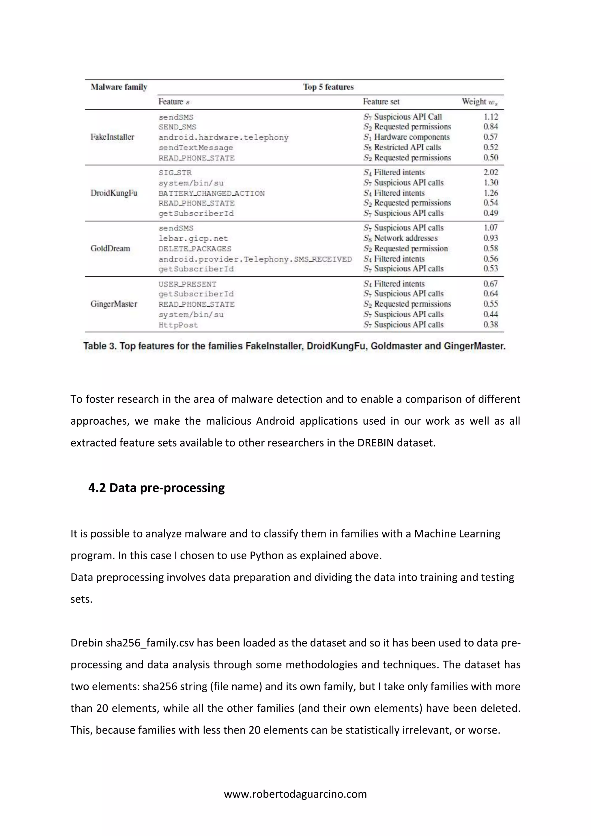
This document discusses using machine learning to classify malware into families based on the DREBIN dataset. It covers: 1. Preprocessing the dataset, including integer encoding and one-hot encoding to convert categorical data to numeric form for modeling. 2. Addressing overfitting by splitting the data into training and test sets and using cross-validation. 3. Using classifiers like Random Forest and SVM with strategies like one-vs-all and one-vs-one to perform multiclass classification of malware families. 4. The process of using binary classifiers for each family first, then combining the results to classify malware into the appropriate family.