This thesis investigates several problems related to eye tracking, including computing a mean gaze path from multiple subjects' eye movements and detecting visual attention without calibration.
To compute a mean gaze path, the thesis develops two methods: 1) A method based on feature networks that produces a graph representation, and 2) A more shape-oriented method that further reduces the data and produces trajectories.
To detect visual attention without calibration, the thesis develops two methods: 1) Using hidden Markov models to passively identify saccade patterns from stimuli, and 2) A smooth pursuit comparison and performance evaluation method.
Both methods for detecting visual attention aim to determine what eye movements a subject is capable of during visual attention in order to


![Chapter 1
Introduction
Eye-movements have been an active subject of study since the nineteenth
century [1], and eye tracking methods were developed later that century.
Despite this fact, the development in the field of eye tracking has been
relatively slow. The early methods of measuring eye positions were highly
intrusive and/or had poor precision. This fact reduced the usability of the
products, and they were therefore mostly used for research. In recent years,
however, the technical level of eye tracking technologies has reached a high
enough level to make the technology truly commercially viable.
As the technology spreads, it opens up for a lot of novel research. The cur-
rently driving forces in this development are marketing research and assistive
technology. As the precision and ease of use for the eyetrackers increase, the
consumer market grows and eye tracking has the potential of becoming a
strong contender as a replacement for the computer mouse in next genera-
tion systems.
Founded in 2001, Tobii Technology is already the market leader in hardware
and software solutions for eye tracking and eye control. This thesis was
sponsored by Tobii, and driven by the current needs in the development of
their main software products.
This chapter will provide more details on eye tracking and some insight on
the methods used, while the next chapter will present the problem formula-
tion.
5](https://image.slidesharecdn.com/fb38d741-da54-4a67-b2ff-89ce75513acc-161017182050/85/main-6-320.jpg)
![1.1 Eye Tracking
Eye tracking relies on and exploits several properties of the human eye, which
will be covered here. The main methods of eye tracking will be explained,
along with the most influential theories on the subject.
1.1.1 The Human Eye
Anatomy
The human eye can be divided into three main layers. These are the fibrous
tunic, the vascular tunic and the nervous tunic [2,3], see Figure 1.1.
Figure 1.1: The anatomy of the eye.
The outermost layer, the fibrous tunic, consists of the cornea and the sclera.
As the name suggests, this layer supports the eye using fibrous tissue. Under
the fibrous tunic lies the vascular tunic, containing the ciliary body, the iris
and the choroid. The ciliary body, mainly consisting of the ciliary muscle, is
responsible for focusing light onto the retina by modifying the shape of the
lens. This layer is also responsible for transporting oxygen to the eye, and
to provide a light-absorbing layer to provide better projection conditions.
6](https://image.slidesharecdn.com/fb38d741-da54-4a67-b2ff-89ce75513acc-161017182050/85/main-7-320.jpg)
![The inner layer, the nervous tunic, is the inner sensoric layer, responsible
for the decoding of the flipped image projected on the retina. The retina
consists of light sensitive rod and cone cells, and their associated neurons.
The axons of these neurons then join together to form the optic nerve. The
area where the optic nerve leaves the eye lacks photo-receptors and is often
referred to as the optic disc, or “the blind spot”.
Outside the optic disc, the retina does not have an even distribution of
photoreceptor cells. The most sensitive area is the macula, and at its center
lies the fovea. This pit-shaped area is the most sensitive to light, and is
responsible for the sharp, central vision. The macula enables high acuity
tasks, such as reading. Since this area has the highest concentration of cone
cells, it is also responsible for the main part of the color vision.
Performance and Control
The width of the fovea is approximately one degree of visual angle, cor-
responding to an area with a radius of about 4.5 mm at normal reading
distance. The acuity of the areas outside it is quite commonly 15-50 per-
cent of the acuity inside it [4], which prevents these areas to participate in
high-acuity tasks. This means that the eye position constantly needs to be
adjusted in order to perform a detailed scan of an object. The scanning
stage of this process is commonly referred to as a fixation, normally lasting
between 150 and 600ms, depending on task [5].
During the fixation, the eye makes a quick decision on where to focus next.
During reading, this is often done in a linear fashion, but the way the scene
is scanned can vary depending on the task [6]. There are many theories on
what drives attention, and how the visual input is processed in the brain.
See [5,7] for an overview.
When the next point of interest has been determined, the eye engages in
a corrective motion in order to transfer focus to this point. This motion
is called a saccade and lasts somewhere between 30 and 120 ms. All sac-
cades are ballistic and therefore cannot be interrupted once initiated [8]. All
movements of the eye are controlled by six different muscles, giving the eye
an excellent ability to quickly and accurately stabilize itself.
7](https://image.slidesharecdn.com/fb38d741-da54-4a67-b2ff-89ce75513acc-161017182050/85/main-8-320.jpg)
![From a Tracking Perspective
The anatomy of the eye, and especially the fact that the eye constantly
changes focus, opens up opportunities for eye tracking. The tracker needs
to estimate the orientation of the eye relative the eye socket in order to deter-
mine the optical axis. Since the location of the fovea relative to the optical
axis is an individual property, the line of gaze and the optical axis do not
necessarily coincide. However, this can be corrected through a calibration
procedure, after which the line of gaze can be determined.
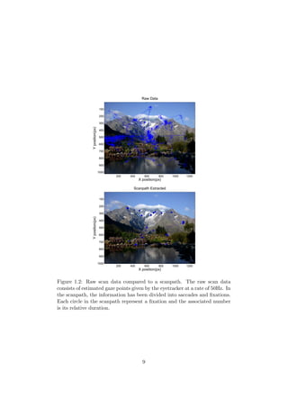
Although the eye has many more types of motion, fixations and saccades
are the most prominent ones during eye tracking. A scanning sequence,
consisting of these two types of motions is known as a “scanpath” [9, 10],
see Figure 1.2.
There are many more types of eye motions, but for one reason or another,
they are all less likely to occur during eye tracking under normal conditions.
For example, smooth pursuit motions occur when the eye is following a
moving object. This might happen during tracking, but studies have tradi-
tionally not included many stimuli triggering such motions. Microsaccades
is another example. They are low-amplitude saccades occurring constantly
during fixations to compensate for the eyes inability to see completely static
images. The low amplitude makes them difficult to measure, since they most
often have smaller magnitude than the measurement noise. For a more elab-
orate discussion of different eye movements, see [8].
1.1.2 Tracking Methods
There are several different methods available when it comes to measuring the
orientation of the eye, but they can be divided into three main categories.
Type one uses in-eye sensors. These are typically glass bodies with some type
of trackable component, such as a magnetic search coil. While these systems
can provide extremely high accuracy measurements suitable for studying the
dynamics of the eye, they are naturally highly invasive and impractical.
Method two estimates the eye position by measuring the electric potential in
the skin directly surrounding the eye. Since this potential is non-stationary,
the method is less suitable for measuring fixed points and slow motions.
Both these techniques measure the orientation of the eye relative the head,
and hence cannot directly determine the location of the object that the
8](https://image.slidesharecdn.com/fb38d741-da54-4a67-b2ff-89ce75513acc-161017182050/85/main-9-320.jpg)
![person is looking at. This absolute position of the gaze point is referred to
as the point of regard. In order to determine it, the head position needs to
be known. This is often accomplished by fixating the subjects head, further
adding to the invasiveness of the first methods. The third method, video-
based corneal reflection, solves this problem. Trackers using this method
typically illuminate the eye with some sort of light (usually infrared). One
or more cameras records the reflection of the light in realtime, and uses
the images, Purkinje Images [11], to estimate the POR. This is not trivial
and involves estimating several parameters to distinguish the head position
from the eye position. It also requires quite elaborate image processing, and
since the eye geometry is directly involved, works differently on each subject.
This technique, although complicated, gives a clear advantage: it’s almost
completely non-intrusive and can estimate POR:s in realtime.
Precision in the corneal reflection trackers are naturally worse than in the
more intrusive ones (the difference is perhaps of order 10-20), but they
still provide good precision (approximately 0.5 degrees). A more detailed
discussion on different tracking techniques is given in [12].
1.1.3 The Scanpath Theory
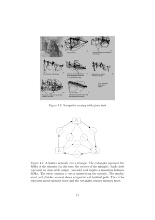
One of the first studies on the sequential nature of the human vision system
was presented in 1967 by Yarbus [13]. He showed that the scanpaths from
the same subject, over the same stimulus, vary with the given task (see
Figure 1.3).
In 1971, Noton and Stark published two articles in Science and Scientific
American [10] [9]. The theories and ideas therein are considered to be some
of the most influential in the field of vision and eye movements [14], and one
commonly referred to as the “scanpath theory”.
This theory extends the work of Yarbus. It presents the human vision sys-
tem as being driven by a top-down process, where the mental image of the
surroundings is pieced together by the information gained through the in-
formation gathered in the scanpath. Noton and Stark also presents and
backs up a theory of how visual attention is directed. They noted that there
are evidence of repetitive patterns (cycles) in most scanpaths (as previously
indicated by Yarbus and others). In the proposed model of the scanning
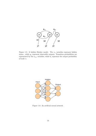
process, the model of visual attention is presented as a “feature network”.
This network is presented as a directed graph containing regions of interest
(ROI:s) as vertices and the edges representing transitions between the differ-
ent states. It is also proposed that individual preferences in the scan order
are present, creating an habitual path in the feature network (see Figure
1.4).
10](https://image.slidesharecdn.com/fb38d741-da54-4a67-b2ff-89ce75513acc-161017182050/85/main-11-320.jpg)
![1.2 Alphabet-Encoded Scanpath Comparison Meth-
ods
One method to perform pairwise scanpath comparisons [15–17] is to use
ROI-based alphabet encoding. By assigning letters to different ROI:s, the
scanpath can be compressed into a string. The scanpath is iterated through,
and fixations within ROI:s generate letters, while fixations outside these
regions are effectively ignored. Successive fixations within the same ROI can
be compressed into one character. In order to compare two scanpaths, string
editing algorithms can be used. Privitera and Stark proposed two different
measurements [15], one temporal and one positional. The first measurement,
Sp, only considers if the two scanpaths contain the same letters. The other
one, Ss uses a string edit distance very similar to the Levenshtein distance
[18].
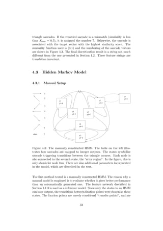
1.3 Hidden Markov Models
Hidden Markov models (HMM:s) are simple state-machine-like statistical
models. The hidden Markov model is a discrete Markov process with un-
known parameters. In a Markov process, each conditional state transfer
probability distribution is conditionally independent of its previous state.
In practice, it means that the probability to transfer to node A in the model
is only dependent on the originating node. There are no “more probable”
paths. This means that a Hidden Markov Model cannot sufficiently model
a proper feature network with a habitual path with more than one step (see
Section 1.1.3). It can, however, approximate such a network if the habitual
path is ignored.
Figure 1.5 shows a graphic presentation of a hidden Markov model with
three states, represented as circles.
1.4 Artificial Neural Networks
Artificial Neural Networks (ANN:s, or simply “Neural Networks”) are math-
ematical constructs used to imitate the biological neural networks found in
the central or peripheral nervous system in humans and animals.
12](https://image.slidesharecdn.com/fb38d741-da54-4a67-b2ff-89ce75513acc-161017182050/85/main-13-320.jpg)
![A biological neural network consists of a set of neurons who interconnect
through chemical synapses and electrical gap junctions. Each neuron has a
number of input signals, called dendrites. When the sum of the input sig-
nals exceed a certain threshold, the neuron sends an output signal through
its axon and the signal propagates through the network. Together, these
neurons can form a single processing unit and it is believed that the in-
terconnection strengths and signal properties of these networks form the
memory structures of the human brain [19].
When simulating the structure of the neural network mathematically, the
neurons are replaced by nodes and the connection strength by weights.
One of the first models of a neural network was the Perceptron, introduced
by Rosenblatt in 1958 [20,21]. This simple ANN consists of an input layer
(called artificial retina) and an output layer. Both the input and output of
the Perceptron is limited to binary vectors. Each input node is connected
to each output node, and the connection strength from input node i to out-
put node j is simulated through a weight, wi,j. This connection strength
combined with a triggering signal results in a stimulation strength, or acti-
vation: aj = I
i=1 xiwi,j, where xi is the i:th input. The output of cell j is
calculated as a function of the activation:
oj =
0 if aj ≤ ϑj
1 if aj > ϑj
(1.1)
This type of function is also referred to as a transfer function. The variable
ϑj is also a parameter of the network. Along with the weights, this parameter
is gradually adjusted through learning. There are several different types
of learning algorithms that apply to ANN:s, but supervised learning is a
common type. When training the network through supervised learning, a
set of example data is used. The system is presented with example data
in iterations. The weights are successively adjusted to minimize the error
output, which is calculated through a performance function. The goal is to
infer the mapping implied by the data into the network.
The relatively simple structure of the Perceptron prevents it to learn arbi-
trarily complex mappings, in fact this early model is only able to learn rules
where the output is a linear transform of the input [22]. This makes it able
to learn logic gate rules such as AND and OR but due to its linearity require-
ment it is unable to learn XOR and other more complex operations [20].
Today, there are many types of neural networks, able to estimate much more
complex functions and to accept a wider set of data. The type of ANN used
14](https://image.slidesharecdn.com/fb38d741-da54-4a67-b2ff-89ce75513acc-161017182050/85/main-15-320.jpg)
![in this thesis is a single-layer feed-forward backpropagation network. It ac-
cepts real numbers as input, and has a single extra layer between input
and output layer, making it able to estimate almost any continuous map-
ping between input and output [23]. The term feed-forward discriminates it
from other types of neural networks, where signals can travel “backwards”
through the layers. Backpropagation describes the type of training algo-
rithm that is used. This technique was first presented by Werbos in [24],
and is (in its original form) a gradient descent algorithm, based on moving
the network weights along the negative gradient of the performance func-
tion. The error is calculated in each output neuron, and the neurons in the
previous layer are then “blamed” according to their connection strength.
Hence the name “backpropagation”. There are now numerous variations
on the original backpropagation algorithm, where improvements have been
made to improve robustness, speed and accuracy of the algorithm.
Examples of variations of the backpropagation algorithm are the Levenberg-
Marquardt (LM) and Resilient Backpropagation(Rprop) algorithms. LM
incorporates Gauss-Newton methods, and is considered being the fastest
algorithm for training feed-forward networks of up to 100 nodes [25]. Rprop
uses a technique to counteract the nonlinearities introduced by sigmoid-
shaped transfer functions in the hidden layers. The simplifications made
in this algorithm reduce memory consumption and hence making it more
suitable for large networks.
1.5 Pairwise Sequence Alignment
Pairwise Sequence Alignment, or Sequence Comparison, is useful in several
fields. In biology, it can be used to compare DNA sequences, taking missing
or superfluous gene insertions into account. It can also be used for comparing
more general text, and forms the basis of the well-known computer program
“diff” [26].
In general, there are two different types of sequence alignments, global and
local alignment. While the global alignment algorithms strive to optimize
the overall match between two strings, the local versions strive to find similar
sub-sequences in sequences that generally are divergent (see Figure 1.7).
A generalized alignment algorithm has three different scoring mechanisms.
An “indel” score (Sin) is added whenever a space has been inserted in either
sequence. A match score (Sma) is applied to all indices in the final alignment
where the letters in both strings are equal. Conversely, a mismatch score
(Smi) is added for all indices where the letters differ.
15](https://image.slidesharecdn.com/fb38d741-da54-4a67-b2ff-89ce75513acc-161017182050/85/main-16-320.jpg)
![Figure 1.7: The difference between global and local sequence alignment.
“Indels” are represented by an underscore.
The Longest Common Subsequence (LCS) is a global sequence alignment
algorithm, with Sma = 1,Smi = 0 and Sin = 0.
In order to solve sequence alignment problems, a dynamic programming
(DP) can be used. Using this technique, the comparison of sub-sequences
are cached in a matrix, and are re-used for the computation of the longer
sequences. This reduces the time complexity significantly.
Including DP, sequence alignment is normally solved in polynomial time,
and there are known ways of constraining the problem space. Mostly known
is the Sakoe-Chiba band [27], which limits the maximum time offset of the
sequences. In its simple form, it has a time complexity in the order of mn,
where n and m is the length of each sequence respectively [28].
1.6 Problem Description
This thesis is divided into several problems, which will here be discussed
separately.
1.6.1 Mean Gaze Path
This problem formulation aims at constructing a new comparison method
for scanpaths that can be utilized to compress a set of scanpaths, from sev-
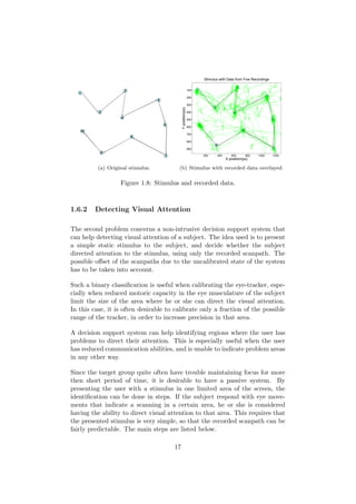
eral different users, into a condensed view. Figure 1.8 shows a stimulus and
corresponding recorded data. Since this stimulus has a very simple and obvi-
ous structure, it provides a good testing ground. The goal with this problem
is to recover the structure of the original stimulus by using only the recorded
data, and to make it as visually clear as possible. Two different techniques
will be evaluated. The first method will utilize clustering to automatically
identify ROI:s from scanpath data, and then build a multigraph to represent
the data. The aim is to present some sort of average feature network (see
Section 1.1.3). The second method will utilize pairwise comparison, focused
on trajectory shapes, and is covered in Section 1.6.4.
16](https://image.slidesharecdn.com/fb38d741-da54-4a67-b2ff-89ce75513acc-161017182050/85/main-17-320.jpg)

![Figure 1.9: The Tobii Technology 1750 eyetracker.
1.7 Experiment Setup
1.7.1 Hardware
In this study, a Tobii 1750 eyetracker was used, see Figure 1.9. This tracker
is based on corneal reflection (see Section 1.1.2). It provides a sampling fre-
quency of 50Hz, and allows for a freedom of head movements in a 30x15x20
cm at 55 cm from the screen.
1.7.2 Scanpath Extraction
The filtering used in this thesis to provide saccade detection and scanpath
extraction was developed by Pontus Olsson [29]. It is an adaptive filtering
based on distance and time measurements. The parameters to this filter,
unless otherwise noted, are meanlength = 5, h = 30. The positions mea-
surements are given in pixels. The coordinate system used is based on a
standard basis, with axes x and y and origo attached to the upper left
corner of the screen.
19](https://image.slidesharecdn.com/fb38d741-da54-4a67-b2ff-89ce75513acc-161017182050/85/main-20-320.jpg)
![Chapter 2
Previous Work
2.1 Mean Gaze Path
There is a lot of work done on how to provide an condensed view over large
sets of eyetracking data. Examples of this are heat maps and clustering of
fixations-rich areas [30, 31]. The ideas employed in this thesis are novel to
my best knowledge.
2.2 Smooth Pursuit Comparison
Comparing eye data has previously mainly been done using Region of Inter-
est (ROI) encoded scanpaths [15, 31]. Usage of this approach significantly
reduces the dimensionality of the scanpath data, and opens up for text based
similarity measures, such as the string edit distance or the longest common
subsequence (LCS or LCSS).
While the ROI method is good for comparing different scanpaths, the method
does not easily lend itself to smooth pursuit comparisons and other eye
movements. Comparing smooth pursuit recordings with occasional saccades
is more closely related to trajectory comparison, a research area which spans
several fields.
In surveillance scenes, trajectories from moving objects such as cars and
people can help detect traffic flow and direction, and discriminate unusual
paths. In this field, a lot of effort has been put into finding a good similarity
measurement between different trajectories. Zhang et al. provide a good
20](https://image.slidesharecdn.com/fb38d741-da54-4a67-b2ff-89ce75513acc-161017182050/85/main-21-320.jpg)
![overview in [32]. In that report, it is concluded that principal component
analysis (PCA) combined with an euclidean distance measurement is best
suited for this. The more complex methods such as dynamic time warping
(DTW) and LCSS methods are considered too computationally costly. The
main reason given is that DTW and LCSS are methods developed to handle
higher-complexity data and to cope with time-axis distortions, which are not
present in the data set. The comparison done above focus on comparison
between whole trajectories, where sub-sequences are ignored, and where the
recorded data has a well-defined time-frame. These differences are signifi-
cant, since eye-tracking data often contain non-linear time distortions, and
significant outliers are commonly present.
In [33], DTW and LCSS are compared with respect to their performance
in comparing multi-dimensional directories with outliers, a data set more
similar to eye tracking data. That paper concludes that LCSS is a good
method in many cases, performing well even in the presence of noise. The
performance problem is once again discussed, and approximation methods
are proposed.
There are many studies done on DTW, LCSS and other related methods.
These can be applied to any type of time-series data. Vlachos et al. [34] de-
scribes how these have been used for matching and classification in numerous
fields (in video, handwriting, video, sign language, etc.).
2.3 Detecting Visual Attention
There is a lot of research performed on automatic detection of salience in
pictures using image processing techniques. When evaluating the perfor-
mance of the proposed models, the triggering of saccades has been used as a
sign of visual attention (see [35,36]). This is a trivial problem since saccades
are easily triggered and detected with humans. The number of fixations on
an area has also been used to evaluate attention [37].
While saccade triggering is a simple and reliable method to use for detect-
ing visual attention, it does require the immediate attention of the viewer.
The passive method developed in this thesis bears little resemblance to this
technique. The techniques used more resembles classical pattern recognition
problems, typically solved using decision support systems. The question at
hand is more which sort of model to use, and what features that are likely
to provide a reliable detection.
21](https://image.slidesharecdn.com/fb38d741-da54-4a67-b2ff-89ce75513acc-161017182050/85/main-22-320.jpg)
![Research in feature extraction of scanpaths, in order to perform decision
support, has been done in several different fields. Saloj¨arvi et al [38] sum-
marize various feature extraction techniques used in the context of reading.
In this paper, words and sentence-ROI:s are given features related to their
relative contextual importance. In this thesis, focus is shifted to non-ROI
methods, since the features need to be translation invariant (since they are
calculated in pre-calibration stage). The use of Markov models to detect
visual attention in repeated exposures to advertisements is covered in [39].
This is also ROI based. The idea to use an automatically generated scan-
path as a universal feature to identify images has been explored [15,40,41].
Rybak et al uses high-saliency edges in the images as a primary feature.
In fact, they try to model the scanpath theory as accurately as possible,
exploiting the physical and neurological properties of humans. While this is
a very interesting approach, providing very high-accuracy detection, it uses
data that is not available in the cases presented here. Also, it depends on
the stateless nature of their feature extractor. This sort of repetitiveness is
not found in humans, due to the arguments found in Section 1.1.3, as well
as others [17].
All these methods are stimuli-driven and therefore requires pre-definitions of
ROI:s or detailed knowledge of the viewers point of gaze. Since the technique
presented in this thesis is performed in an uncalibrated stage, the methods
need to be more data than stimuli driven. There is some work found on a
data-driven approach in [31] and [15]. In the Pritivera and Stark paper, the
idea is to generate ROI:s from a pair of scanpaths using clustering, and then
to use ROI-encoded strings to measure similarity.
In this thesis, the focus will be turned away from the ROI-encoded strings,
and instead concentrated on the detection of saccades. The saccade trig-
gering, however, will not be directly measured. Instead, the theory is that
the saccade signature of a scanpath can be used to identify an image scan-
ning. By manually defining a signature or statistically producing one from
recorded scanpaths, matching can be performed. To the best of my knowl-
edge, this is the first time this principle has been used when comparing
scanpaths searching for visual attention.
22](https://image.slidesharecdn.com/fb38d741-da54-4a67-b2ff-89ce75513acc-161017182050/85/main-23-320.jpg)
![Chapter 3
Mean Gaze Path
By identifying ROI:s through clustering and constructing a transition graph,
this method provides an overview similar to a heatmap, but it also adds tran-
sition statistics and can create clusters with different directional properties.
It aims at resembling the feature network presented in [9].
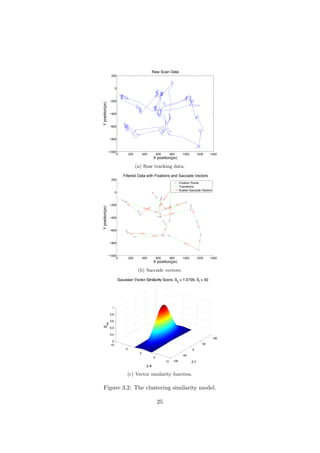
3.1 Features
Aside from the scanpath extraction covered in Section 1.1.3, the saccade
vectors in between fixations are also used. If f[n] represents the n:th fixation
vector with x and y positions as described in Section 1.7.2, these vectors can
be obtained through the expression v[n] = f[n]−f[n−1]. How these features
relate to the original data is illustrated in Figure 3.2(b).
3.2 Distance Measurement
The distance measurement used in the clustering process can be a simple eu-
clidean distance, which is a measure of distance between the fixation points.
The negative effect that it has is that direction is not taken into account.
If two clusters of fixations are located close to each other, and they rep-
resent movement in two different directions, one might wish to keep them
separated. This is illustrated in Figure 3.1.
23](https://image.slidesharecdn.com/fb38d741-da54-4a67-b2ff-89ce75513acc-161017182050/85/main-24-320.jpg)
![1
2
Figure 3.1: A hypothetical feature network over several individuals. The
nodes represent fixation clusters and the vertices represent common transi-
tions. The clusters numbered as 1 and 2 might be close to each other, but
they represent different movements.
Computing the similarity (Snk) between two saccade vectors, with index
n and k, can be done by using a Gaussian score, relative to the euclidian
distance and angle deviations of the two vectors:
Snk = e−(∆θ/sθ)2−(∆l/sl)2
(3.1)
, where ∆θ = arctan(dvy/dvx), ∆l = |f[n] − f[k]|, z = dvx + i · dvy
and dv = v[n] − v[k]. This measurement has two parameters, sθ and sl.
They are angle and distance tolerances, respectively. Note that separating
these two variables allows to individually tune the sensitivity to deviations
in both saccade directions and distance. An example plot of the similarity
function is given in Figure 3.2(c). The distance between fixations is later
calculated through Dnk = S−1
nk .
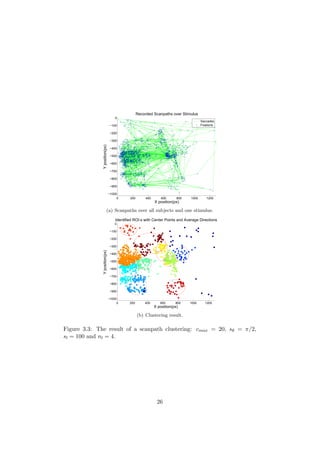
3.3 Clustering
In order to identify the ROI:s in the graph, clustering of fixations is employed
over all scanpaths involved. Any type of clustering can be applied to this
problem, but it’s generally better to use a method which doesn’t require
the number of clusters to be known. The scanpath-specific ideas found in
Santella and DeCarlo [30] can also be used.
A hierarchical clustering was used in this thesis. Linkage was done by using
unweighted average distance (UPGMA) and the actual clustering was done
with a simple tree cut with an upper limit of the number of clusters (cmax).
Finally, all clusters containing less than nl fixations where removed.
24](https://image.slidesharecdn.com/fb38d741-da54-4a67-b2ff-89ce75513acc-161017182050/85/main-25-320.jpg)

![Since the study was performed with subjects with normal vision, it had
a different structure. Instead of asking people to ignore certain images,
they were presented with stimuli triggering widely different patterns. These
images were chosen to create scanpaths of varying types. The results of
this study relies on the fact that this reliably recreates the scanpaths of
a subject not seeing the stimulus. The stimuli used are varied. Some are
designed to trigger search-like patterns, some are simple stimulus with a
few high-saliency areas, triggering specific scanning patterns. The final type
consist of landscape-type low-saliency images, triggering random patterns.
The subjects where chosen at random, and they were asked to pay attention
to the patterns shown to them. Each person was presented with 18 im-
ages, displayed with a duration of six seconds each. Every second of these
contained three words (each one short enough to require only one fixation),
positioned in the corners of a triangle. The other images were selected at
random, designed to trigger a wide array of different type of saccade pat-
terns (see Figure 4.1). The main reason why words are chosen is to increase
the variance in the generated saccades, since the target user group might
not have the high accuracy of the test group. The total number of images
in the study were 270.
The decision support systems were evaluated through a classification test.
They were fed with both triangle and non-triangle patterns, and their per-
formance was measured through their ability to discriminate between these
two types. The correct classification rate, Rc, is defined as
Rc =
correct classifications
total number of pattern processed
(4.1)
4.2 Feature Extraction
As already mentioned, the ideas employed here are mostly based on Noton
and Starks scanpath theory (see Section 1.1.3). Since, according to this
theory, all transitions between ROI:s will trigger saccades, there should be
some kind of saccadic profile associated with each stimulus. This profile
could of course change over time, if the user develops a habitual path. If
temporal order is taken out of context, such a habitual path could have
minor effect, since the high-salience areas of the stimulus stay constant. This
should have higher effect on a carefully chosen profile. The other implication
showing that this should work is that the studies performed by Pieters et
al [39] show that scanpaths obey a stationary, reversible, first-order Markov
process.
30](https://image.slidesharecdn.com/fb38d741-da54-4a67-b2ff-89ce75513acc-161017182050/85/main-31-320.jpg)

![In order to select such a profile, consider a normalized frequency binning
of the lengths and angles of the different saccade vectors (see Figure 4.2).
These two feature vectors are fixed length, suitable for fixed-topology neural
networks. In this extraction, the angles and lengths of each saccade v[n] is
computed through l = |z|, θ = arg(z), where z = v[n]x + i · v[n]y, i.e a polar
representation.
200 400 600 800 1000 1200 1400
−700
−600
−500
−400
−300
−200
−100
Original Scanpath
X position(px)
Yposition(px)
(a) Recorded scanpath from a triangle stim-
ulus.
1 2 3 4 5 6 7 8 9 10
0
0.05
0.1
0.15
0.2
0.25
0.3
0.35
0.4
0.45
Normalized Angle Features, θ
max
=3.1416
Bin Number
RelativeFrequency
(b) Angle binning. Angles range from 0 to
Θmax.
1 2 3 4 5 6 7 8 9 10
0
0.05
0.1
0.15
0.2
0.25
0.3
0.35
0.4
0.45
Normalized Length Features, l
max
=400
Bin Number
RelativeFreqency
(c) Length binning. Possible lengths range
from 0 to lmax.
Figure 4.2: Feature extraction from a scanpath, based on frequency binning.
Since normalized binning is used, each bin represent an equal range. Length
bin i has a span from (i − 1) ∗ lmax/10 to i ∗ lmax/10. Likewise, angle bin i
has a span from (i − 1)Θmax/10 to i ∗ Θmax/10.
Another approach is to use temporal ordering in the feature vector, and
then use a decision support system that takes this into account. Here, this is
done through discretizing each saccade via a “best match” procedure. Using
integer encoding, each target vector (as well as the mismatch) is associated
with a number. Six different target vectors (1 − 6) are used to detect in-
32](https://image.slidesharecdn.com/fb38d741-da54-4a67-b2ff-89ce75513acc-161017182050/85/main-33-320.jpg)


![system, as discussed in Section 4.3.1. The classification rate of the automatic
model is higher than the manual model, but still far from perfect. In order
to evaluate if the stateless (markovian) model of scanpaths holds, another
transformation to feature space will be tested in the next section. The
classification mechanism is also changed to a neural net, which supports
fixed length feature vectors.
4.4 Artificial Neural Network
In order to test the fixed length feature vectors discussed in Section 4.2,
a neural network approach is employed. For reasons already outlined in
Section 1.4, a single-layer feed-forward backpropagation net is chosen.
The two fixed-size binning-based features mentioned in Section 4.2 are con-
catenated to construct the final feature vector. The lengths and angles are
each binned into 10 equally sized bins, the lengths ranging from 0 to 700, and
the angles from 0 to 2π. Log-sigmoid transfer functions, logsig(n) = 1
1+e−n ,
are used in the hidden and output layers to map the similarity index to an
interval of R ∈ [0, 1]. This similarity value is later thresholded at 0.5 to
indicate match or mismatch. Half of the data is selected as training data,
and one fourth as validation data. The last data is used as test data. Each
set is sampled evenly from the original data set. The validation data set is
used to provide a stopping condition.
Since no performance problems are encountered, the Levenberg-Marqhart
training algorithm is used. The number of nodes in the hidden layer is varied,
and the performance of the net is deemed to be good for most settings, when
the number of nodes lies between 10 and 40. The variation is not presented
here, since the variance between runs is greater than the variance caused by
adjusting the number of nodes.
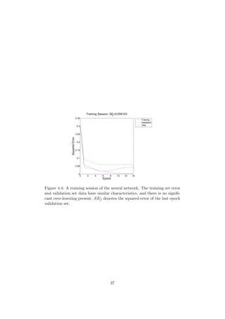
The correct classification rate, Rc, seems to vary between 0.85 and 1.0, an
example result is shown in Figure 4.4. In this run, 30 nodes were used in
the hidden layer. The network correctly classified 67 out of the 68 training
patterns, giving a hit rate of Rc = 67/68 ≈ 0.9853.
4.5 Conclusions
When it comes to detecting visual attention, the neural network outperforms
the HMM approach. Since the feature vectors being used are significantly
different, it is not certain whether the difference depends on the ANN:s abil-
ity to capture more dynamics or if the feature extraction plays a major role.
If HMM:s are used, there is no need to manually construct a model, since
the automatically trained one offers better performance and less settings.
The correct classification rate of the ANN is very high, and it could very
well be used as a decision support system in the described situation.
36](https://image.slidesharecdn.com/fb38d741-da54-4a67-b2ff-89ce75513acc-161017182050/85/main-37-320.jpg)
![Chapter 5
Smooth Pursuit Comparison
The nature of the smooth pursuit (SP) differs from the standard saccade-
fixation pattern. When engaged in this sort of movement, the eye performs
a smooth sweeping in order to follow an object in motion [42]. There are
studies indicating that the compensation system used during smooth pursuit
can be modeled as a closed-loop control system with prediction, but the
exact dynamics of such a model are not quite clear [43–45]. Most sources
indicate that the initial delay of these movements is about 100ms. Many
sources also agree that the mind uses a predictive model to decide on when
to change the tracking method, and for instance initiate corrective saccades
[46].
The smooth shape of SP motions, along with the relatively low time and
angular offset from the target shape (see [45]), makes it easy to compare the
gaze trajectory with the stimulus trajectory.
If the gaze position is known, a simple euclidian distance match can be
made, possibly incorporating some sort of logic in order to compensate for
time offsets. Since the application covered here operates in a pre-calibration
state, however, the match needs to be done differently.
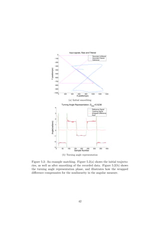
5.1 Feature Extraction
In order to provide a translation invariant representation, the eye trajectories
are transformed into arc length vs turning angle representation [47]. Let
p[n] (where n is discrete time (samples)) represent the recorded gaze point
at sample n. Let N be the number of samples in the sequence. Also, let
38](https://image.slidesharecdn.com/fb38d741-da54-4a67-b2ff-89ce75513acc-161017182050/85/main-39-320.jpg)
![p[n] = p[0] ∀ n < 0. Then the length l[n] = n
k=0 |p[k] − p[k − 1]|. In this
chapter, time will be used instead of arc length, but this measure will be
used during the second mean gaze path extraction.
The turning angle is calculated as the angle to an absolute reference vec-
tor (vref ). This reference vector is compared to the vectors between sam-
ple points in the recorded data. These vectors are calculated through
v[n] = p[n + 1] − p[n]. The last vector in the recorded data is interpo-
lated such that v[n] = v[N − 1] ∀ n ≥ N. The dot product cannot be used
to calculate the turning angle. This is due to the fact that the dot prod-
uct calculates the (signless) acute angle between two vectors, and doesn’t
take direction into account. To compensate for this fact, the “2D cross
product” [48] is used to figure out the signed angle between two vectors:
Θs = s12 arctan v1·v2
|v1||v2| , where s12 = sgn(v1xv2y − v1yv2x). This method
is somewhat similar to the four quadrant inverse tangent, commonly re-
ferred to as the atan2. By utilizing a variable reference vector, however, the
discontinuity present around π,−π in the atan2 method can be arbitrarily
shifted around the unit circle. If there is prior knowledge of the recorded eye
data, this fact can be utilized to move the discontinuity away from common
vectors, which reduces noise and increases robustness of the matching.
Figure 5.1: Noise-reducing wrapped distances. The upper and lower lines in
the figure are Θd+ and Θd− respectively. The dots represent measurements,
Θ1 and Θ2, in three different cases. The measurements involved in direct,
wrapped and inverse wrapped distances are shown in turn from left to right.
The minimum of these distances are chosen in the method proposed.
Another method that can be utilized in order to reduce the noise is to employ
a “closest distance” measurement. Let Θref = arctan(vrefy/vrefx). Then
the turning angle measurement has a discontinuity around Θd+ = Θref + π
and Θd− = Θref −π. If two turning angle measurements, Θ1 and Θ2 are to be
compared, the minimum of three distances can be used: direct, wrapped and
inverse wrapped distances, see Figure 5.1. The direct distance is calculated
through Ddirect = |Θ1 − Θ2|. The wrapped distance is calculated through
Dwrap = |Θd+ − Θ1| + |Θd− − Θ2|. The inverse wrapped distance is likewise
39](https://image.slidesharecdn.com/fb38d741-da54-4a67-b2ff-89ce75513acc-161017182050/85/main-40-320.jpg)
![calculated through Diwrap = |Θd+ − Θ2| + |Θd− − Θ1|. Since Θ1 and Θ2 are
bounded by Θd− < Θn ≤ Θd+, the wrapped distances can be simplified to
Dwrap = Θd+−Θd−−T12 and Diwrap = Θd+−Θd−−T21, where T12 = Θ1−Θ2
and T21 = Θ2 − Θ1. When taking the minimum of these two distances,
the symmetry between T12 and T21 and the fact that Θ1 and Θ2 have the
same bounds as Dwrap and Diwrap can be utilized. This helps simplify the
minimization expression,
min
Dwrap
Diwrap
= min
Θd+ − Θ1 + (−(Θd− − Θ2))
Θd+ − Θ2 + (−(Θd− − Θ1))
= Θd+−Θd−−|Θ1−Θ2|
. The total expression, calculating the closest distance becomes
D12 = min
Ddirect
Dwrap
Diwrap
= min
|Θ1 − Θ2|
Θd+ − Θd− − |Θ1 − Θ2|
.
If a reference vector of vref = [1, 0] is used, the extracted signed angle has
a discontinuity around Θd+ = π and Θd− = −π, where the measurement
wraps around. The above expression then takes the following form:
D12 = min
|Θs1 − Θs2|
2π − |Θs1 − Θs2|
. This special case is mentioned in Vlachos et al [49].
5.2 Matching
When performing this matching, a reference path pref [n] is going to be
compared to an actual recording p[n]. The recording p[n] is actually a filtered
version of the raw scan data. The filtering used is a zero-phase forward and
reverse filtering using a third order butterworth filter with ωn = 0.05 [50,51].
The start and end transients are suppressed using a linear interpolation with
a length of np = 200 samples. The filtering is done separately for the x and y
sequences, each representing the data from one of the two spatial dimensions
present.
As mentioned in Section 5.1, each trajectory is transformed from euclidian
vs time space into turning angle vs time space. The matching is then done
using a maximal angular difference, D12 ≤ Dmax. This measurement only
takes direction into account, so it is unable to detect sudden offset shifts in
40](https://image.slidesharecdn.com/fb38d741-da54-4a67-b2ff-89ce75513acc-161017182050/85/main-41-320.jpg)
![the sequence. The offset of the tracker is usually constant, so such a jump
would indicate something abnormal, so the matcher needs to address this.
The detection of non-stationary translations in done with the help of the
following procedure:
Let M be the set of indices where a direction match is present. The euclidean
distance between the reference and recorded path is computed using δp[n] =
pref [n]−p[n], n ∈ M. The mean is then deducted from the x and y sequences
separately.
xnorm[n] = δp[n]x − mean(δp[n]x)
ynorm[n] = δp[n]y − mean(δp[n]y)
The length deviation is computed through ∆d = x2
norm + y2
norm. Finally,
all match indices where the length deviation exceeds dmax are pruned. When
these indices have been removed, the final similarity score is calculated
through S = size(M)
N .
An example match is shown in Figure 5.2 and Figure 5.3.
5.3 Evaluation
Performance evaluation was done with a group of ten people, selected at
random. These subjects were presented with a video of a moving dot, trav-
eling across the screen with a speed of approximately 20 degrees per second,
without acceleration. For a discussion on the proper stimuli for this type of
study, see [52].
The stimulus moved in the same pattern as shown in Figure 5.3, and the
recording started from the first moment that the dot was shown, thus in-
cluding the initial transient when the subject redirects gaze to the moving
stimulus. The duration of each recording was ten seconds.
Each recording, n, was processed in order to extract the similarity score.
The resulting score sequence containing similarity scores for all subjects is
here denoted sh[n]. The reference sequence was based on the same reference
path, but with random gaze data. Each reference sequence consisted of a
set of fixations drawn from a uniform distribution, with the same interval
as the screen coordinates. The resulting similarity sequence is called sr[n].
The matching parameters being used were N = 3, ωn = 0.05, dmax =
200, Dmax = π/6. Using these parameters, the score for the recorded data,
41](https://image.slidesharecdn.com/fb38d741-da54-4a67-b2ff-89ce75513acc-161017182050/85/main-42-320.jpg)
![0 50 100 150 200 250 300 350
−150
−100
−50
0
50
100
150
200
Match Point Offset after Realignment, dmax
=200
Matching Index
Distance(px)
x
norm
[n]
ynorm
[n]
∆ d
d
max
(a) Translation detection
0 200 400 600 800 1000 1200 1400
−1000
−900
−800
−700
−600
−500
−400
−300
−200
−100
0
Reference Signal with Final Matching, S =0.87179
X position(px)
Yposition(px)
Reference Signal
Recorded Signal
Match Vectors
(b) Final matching
Figure 5.3: An example matching. Figure 5.3(a) depicts the different offsets
present in the match, and the upper limit. Figure 5.3(b) shows the final
matching points.
43](https://image.slidesharecdn.com/fb38d741-da54-4a67-b2ff-89ce75513acc-161017182050/85/main-44-320.jpg)

![Chapter 6
Mean Path Revisited
In this chapter, an attempt is made to determine a mean gaze with fewer
graph-like properties than the representation covered in Chapter 3. The goal
is to find one or a few representative paths through the stimulus and to show
the path of an “average user”. This is not an exact science, since there is no
really good definition of what a “mean path” is or represents. This chapter
will discuss one solution to this problem, which generates representative
paths for certain types of data. While the previous method focused on
ROI:s, this approach will use features more related to the shape of the
scanpaths.
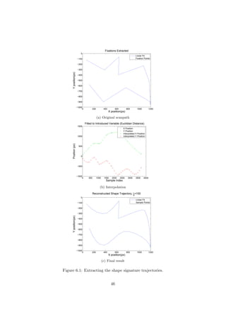
6.1 Feature Extraction
Since this method operates on scanpaths, the fixations are extracted like de-
scribed previously. In order to compare the shape of the different scanpaths,
they are re-sampled with an equal space interpolation. Let N denote the
total number of fixations in the scanpath being currently processed. The
length of each section is computed as described in Section 5.1. The total
length of the scanpath, l[N], is used to compute the interpolation. The x
and y scanpath sequences (f[n]x and f[n]y) are then independently resam-
pled using a cubic spline interpolation, using equally spaced points along
the length span l ∈ [0, l[N]]. The distance between consecutive points in
the resampled sequences is denoted ld. The produced sequence, s[n] is a
trajectory representing the shape of the original scanpath. Figure 6.1 gives
a graphical view of the process.
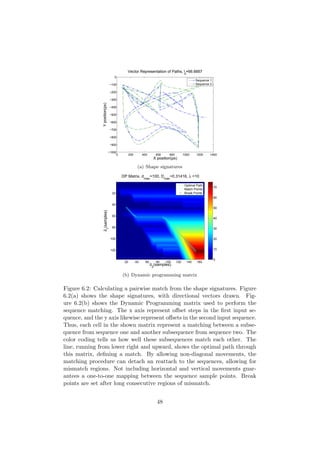
45](https://image.slidesharecdn.com/fb38d741-da54-4a67-b2ff-89ce75513acc-161017182050/85/main-46-320.jpg)
![6.2 Path Joining
6.2.1 Finding Matching Regions
In order to extract matching regions among the set of extracted shape sig-
natures, a sequence matching algorithm is used (see Section 1.5). This is
done for each pair of sequences in the set. The sequence matching algo-
rithm being used differs a bit from the standard LCS. First, the scoring is
not constrained to LCS, but can be set arbitrary. Second, there is a rule
considering “indels”. If more than λ consecutive “indels” appear, this is
considered being a break in the sequence. This allows the algorithm to split
a single pairing of two sequences into several matching sub-regions. The
traceback of the DP matrix is done from the maximum point, and stops
when zero similarity is reached. This ensures selection of the best matching
sequence, not penalizing trailing and leading mismatch sections.
Let V (i, j) denote the optimal alignment for the prefixes s1[1..i] and s2[1..j]
of the two shape signatures s1 and s2. Let Sm denote the match score:
Sm = Sma upon match and Sm = Smi upon mismatch between s1[i] and
s2[j]. Also let Sin1 and Sin2 denote the “indel” costs of sequence one and
two respectively, then
V (i, j) = max
0
V (i − 1, j − 1) + Sm
V (i − 1, j) + Sin2
V (i, j − 1) + Sin1
(6.1)
.
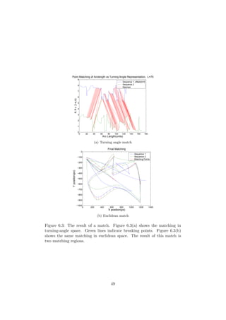
The matching criteria for two sequences is given by the wrapped angle di-
rection measurement Θs described in Section 5.1, along with a maximum
allowed euclidean distance, dmax. See Figure 6.2 and Figure 6.3. The scores
used in this chapter are Sma = 1, Smi = −1 and Sin1 = Sin2 = −1.
Complexity
This method has a high computational complexity. The number of pairs
that needs to be matched is n(n−1)
2 , where n is the number of sequences in
the set. Since the sequence length is unbounded, it is not feasible to utilize
a Sakoe-Chiba limit (see Section 1.5), and the time needed to compute the
LCS is quadratic to the trajectory size.
47](https://image.slidesharecdn.com/fb38d741-da54-4a67-b2ff-89ce75513acc-161017182050/85/main-48-320.jpg)
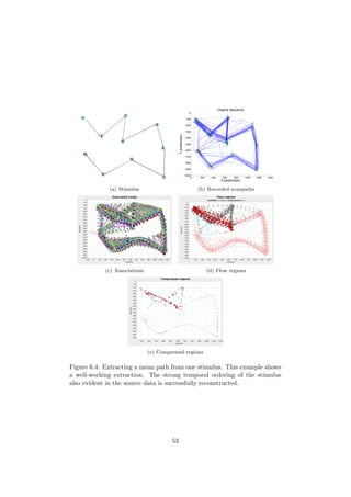
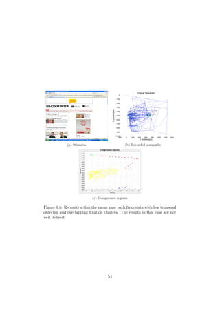
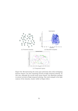
![6.3 Reconstruction
In order to reconstruct a mean gaze path from the performed pairwise match-
ing, three algorithms are developed. The first one uses a voting-based tech-
nique to compute how well each trajectory node is connected to other nodes.
The second algorithm utilizes this information to join areas with similar con-
nection index to each other, forming regions. The final algorithm compresses
these regions into single trajectories.
6.3.1 Connection Index
When the pairwise matching is done, each node within the matching set is
connected with its matching neighbors, from the set in whole. Each node is
then given a connection index, ci[m]. This index represents how well asso-
ciated the node with index m is with other nodes. The connection index is
computed through counting the total number of other nodes that are con-
nected, directly or indirectly, through trajectory or similarity connections.
The algorithm being used follows these links, expanding breadth first, stop-
ping when an already visited trajectory is encountered. Let Sn denote the
set of all nodes among all shape trajectories. Let M = |Sn| denote the car-
dinality of Sn, and Sc(n) the set of nodes counting towards the connection
index for the node named n. Then Sc(n) can be computed as given by Algo-
rithm 1. The connection index ci[m] is then defined as ci[m] = |Sc(Sn[m])|
(the size of Sc for node m).
Algorithm 1 Sc(n)
Require: A node n.
1: Sc ← ∅
2: visited trajectories ← ∅
3: for all nodes m connected to n do
4: if m:s trajectory ∈ visited trajectories then
5: break
6: else
7: add m:s trajectory to visited trajectories
8: add m and Sc(m) to Sc
9: end if
10: end for
50](https://image.slidesharecdn.com/fb38d741-da54-4a67-b2ff-89ce75513acc-161017182050/85/main-51-320.jpg)
![6.3.2 Flow Regions
When the connection index is computed for each node, a type of “flood fill” is
applied. Nodes with similar connection index are grouped together, using a
fill tolerance level, ftol. Let U denote the set of nodes who are candidates for
the “flood fill”, and Ff (n, U) the filled set, called a “flow region”. Also, let
ci denote the connection index of the original node. The algorithm starts by
filling U with all available nodes. One node at a time is picked from the set,
and is used as the source for a flood fill. If the connection index of the source
node is lower than minConn, the node is dropped and ignored. When there
are no free nodes left, the whole set is effectively divided into different flow
regions. Finally, all regions consisting of less than minRegionSize nodes
are removed. The flood fill is described by Algorithm 2.
Algorithm 2 Ff (n, ci, U, ftol)
Require: A node n, a set U, an integer ci and an integer ftol.
1: Ff ← n
2: freeNodes ← U
3: for all nodes m connected to n do
4: if m ∈ free nodes and |ci[m] − ci| < ftol then
5: add m to Ff
6: add Ff (m, ci, U, ftol) to Ff
7: end if
8: end for
6.3.3 Region Compressing
In order to reduce the width of the flow regions, a traversal of each region
is performed. In this traversal, directly connected nodes with identical flow
index are compressed by replacing them with a node positioned in their
euclidean mean position.
6.3.4 Reordering
Since there is no time information available in the resulting set after region
compression, this needs to be constructed. It can be accomplished by using
a brute force traveling salesman problem (TSP) approach, or some other
method of shape reconstruction, such as the one proposed by Floater in [53].
The TSP method is used here, since it does not need start or endpoints to
be specified, something that is also lost in the compression phase.
51](https://image.slidesharecdn.com/fb38d741-da54-4a67-b2ff-89ce75513acc-161017182050/85/main-52-320.jpg)

![Chapter 7
Conclusions and Future
Work
7.1 Mean Gaze Path
This thesis covers potential solutions to several problems present at Tobii
Technology. One of these problems is the construction of a “mean gaze
path”. This problem was addressed from two directions. One was heav-
ily based on Noton and Starks [9,10] scanpath theory. This fixation-based
representation proved well-defined and easy to compute, providing a good
overview. In an attempt to leave the feature network approach, and focus on
the shapes present in the recordings, an approach based on pairwise sequence
alignment and shape-related features was developed. This method proved
to have high computational complexity and was not well-defined for all sorts
of input, but proved useful for input data with strong temporal ordering and
well-separated fixation clusters. The main problem in the second method,
that needs to be addressed, is finding a way of preserving the temporal infor-
mation in the shape signatures. The pairwise comparison technique needs
to be replaced or modified in order to reduce the computational complexity.
One optimizing technique is to use string-editing techniques that operate on
several sequences at once [54].
The conclusion in this area is that both methods are useful, but the former
method described in Chapter 3 is preferred for general data, due to the
reasons outline here and in Section 6.4.
56](https://image.slidesharecdn.com/fb38d741-da54-4a67-b2ff-89ce75513acc-161017182050/85/main-57-320.jpg)
![Bibliography
[1] R. J. K. Jacob and K. S. Karn, “Commentary on Section 4. Eye tracking
in human-computer interaction and usability research: Ready to deliver
the promises,” The Mind’s Eyes: Cognitive and Applied Aspects of Eye
Movements. Oxford: Elsevier Science, 2003.
[2] “Eye diagram,” http://en.wikipedia.org/wiki/Image Schematic
diagram of the human eye en.svg, 2007.
[3] C. S. McCaa, “The Eye and Visual Nervous System: Anatomy, Physi-
ology and Toxicology,” Environmental Health Perspectives, vol. 44, pp.
1–8, 1982.
[4] R. J. K. Jacob, “Eye tracking in advanced interface design,” Virtual
Environments and Advanced Interface Design, pp. 258–288, 1995.
[5] A. Duchowski et al., Eye Tracking Methodology: Theory and Practice,
Springer, 2003.
[6] A. L. Yarbus, “Eye movements during perception of complex objects,”
Eye Movements and Vision, pp. 171–196, 1967.
[7] A. H. C. van der Heijden, Selective Attention in Vision, Routledge,
1992.
[8] A. Duchowski et al., Eye Tracking Methodology: Theory and Practice,
pp. 43–51, Springer, 2003.
[9] D. Noton and L. Stark, “Scanpaths in saccadic eye movements while
viewing and recognizing patterns,” Vision Research, vol. 11, no. 9, pp.
929–42, 1971.
[10] D. Noton and L. Stark, “Eye movements and visual perception,” Sci-
entific American, vol. 224, no. 6, pp. 35–43, 1971.
[11] H. D. Crane, “The Purkinje Image Eyetracker, Image Stabilization,
and Related Forms of Stimulus Manupulation,” Visual Science and
Engineering: Models and Applications, pp. 13–89, 1995.
58](https://image.slidesharecdn.com/fb38d741-da54-4a67-b2ff-89ce75513acc-161017182050/85/main-59-320.jpg)
![[12] A. Duchowski et al., Eye Tracking Methodology: Theory and Practice,
pp. 55–65, Springer, 2003.
[13] A. L. Yarbus, Eye Movements and Vision, Plenum Press New York,
1967.
[14] C. M. Privitera, “The scanpath theory: its definition and later devel-
opments,” Proceedings of the SPIE, vol. 6057, pp. 87–91, 2006.
[15] C. M. Privitera and L. W. Stark, “Algorithms for defining visual
regions-of-interest: comparison with eye fixations,” IEEE Transac-
tions on Pattern Analysis and Machine Intelligence, vol. 22, no. 9, pp.
970–982, 2000.
[16] L. W. Stark and C. Privitera, “Top-down and bottom-up image pro-
cessing,” International Conference on Neural Networks, vol. 4, 1997.
[17] S. A. Brandt, “Spontaneous Eye Movements During Visual Imagery
Reflect the Content of the Visual Scene,” Journal of Cognitive Neuro-
science, vol. 9, no. 1, pp. 27–38, 1997.
[18] V. I. Levenshtein, “Binary Codes Capable of Correcting Deletions,
Insertions and Reversals,” Soviet Physics Doklady, vol. 10, pp. 707,
1966.
[19] M. J. Denham, “The Dynamics of Learning and Memory: Lessons from
Neuroscience,” Emergent Neural Computational Architectures based on
Neuroscience, 2001.
[20] H. Abdi, “A neural network primer,” Journal of Biological Systems,
vol. 2, no. 3, pp. 247–283, 1994.
[21] F. Rosenblatt, “The perceptron: a probabilistic model for information
storage and organization in the brain.,” Psychol Rev, vol. 65, no. 6, pp.
386–408, 1958.
[22] F. Rosenblatt, Principles of neurodynamics, Spartan Books, 1962.
[23] S. Tamura and M. Tateishi, “Capabilities of a four-layered feedforward
neural network: fourlayers versus three,” IEEE Transactions on Neural
Networks, vol. 8, no. 2, pp. 251–255, 1997.
[24] P. J. Werbos, Beyond Regression: New Tools for Prediction and Analy-
sis in the Behavioral Sciences, Ph.D. thesis, Harvard University, 1974.
[25] H. Demuth and M. Beale, “Neural Network Toolbox,” The MathWorks
Inc.: Natick, 1993.
59](https://image.slidesharecdn.com/fb38d741-da54-4a67-b2ff-89ce75513acc-161017182050/85/main-60-320.jpg)
![[26] J. W. Hunt and M. D. McIlroy, “An algorithm for differential file
comparison,” Computing Science Technical Report, 1975.
[27] H. Sakoe and S. Chiba, “Dynamic programming algorithm optimization
for spoken word recognition,” IEEE Transactions on Acoustics, Speech,
and Signal Processing, vol. 26, no. 1, pp. 43–49, 1978.
[28] D. Maier, “The Complexity of Some Problems on Subsequences and
Supersequences,” Journal of the ACM (JACM), vol. 25, no. 2, pp.
322–336, 1978.
[29] P. Olsson, “Real-time and Offline Filters for Eye Tracking,” M.Sc.
thesis, Royal Institute of Technology, Apr. 2007.
[30] A. Santella and D. DeCarlo, “Robust clustering of eye movement
recordings for quantification of visual interest,” Eye Tracking Research
& Applications (ETRA) Symposium, 2004.
[31] J. Heminghous and A.T. Duchowski, “iComp: a tool for scanpath
visualization and comparison,” Proceedings of the 3rd symposium on
Applied perception in graphics and visualization, pp. 152–152, 2006.
[32] Z. Zhang, K. Huang, and T. Tan, “Comparison of Similarity Mea-
sures for Trajectory Clustering in Outdoor Surveillance Scenes,” Pro-
ceedings of the 18th International Conference on Pattern Recognition
(ICPR’06)-Volume 03, pp. 1135–1138, 2006.
[33] M. Vlachos, G. Kollios, and D. Gunopulos, “Discovering similar multi-
dimensional trajectories,” Proceedings. 18th International Conference
on Data Engineering, pp. 673–684, 2002.
[34] M. Vlachos, M. Hadjieleftheriou, D. Gunopulos, and E. Keogh, “In-
dexing multi-dimensional time-series with support for multiple distance
measures,” Proceedings of the ninth ACM SIGKDD international con-
ference on Knowledge discovery and data mining, pp. 216–225, 2003.
[35] D. Parkhurst, K. Law, and E. Niebur, “Modeling the role of salience in
the allocation of overt visual attention,” Vision Research, vol. 42, no.
1, pp. 107–123, 2002.
[36] S. P. Liversedge and J. M. Findlay, “Saccadic eye movements and
cognition,” Trends in Cognitive Science, vol. 4, no. 1, pp. 6–13, 2000.
[37] A. Login, I. Registration, P. Registration, S. Map, and S. Areas,
“Like more, look more. Look more, like more: The evidence from eye-
tracking,” Journal of Brand Management, vol. 14, pp. 335–342, 2007.
60](https://image.slidesharecdn.com/fb38d741-da54-4a67-b2ff-89ce75513acc-161017182050/85/main-61-320.jpg)
![[38] J. Salojarvi, K. Puolamaki, J. Simola, L. Kovanen, I. Kojo, and
S. Kaski, “Inferring relevance from eye movements: Feature extraction
(Tech. Rep. No. A82). Helsinki University of Technology,” Publications
in Computer and Information Science, 2005.
[39] R. Pieters, E. Rosbergen, and M. Wedel, “Visual Attention to Repeated
Print Advertising: A Test of Scanpath Theory,” Journal of Marketing
Research, vol. 36, no. 4, pp. 424–438, 1999.
[40] I. A. Rybak, V. I. Gusakova, A. V. Golovan, L. N. Podladchikova, and
N. A. Shevtsova, “A model of attention-guided visual perception and
recognition,” Vision Research, vol. 38, no. 15-16, pp. 2387–2400, 1998.
[41] M. Kikuchi and K. Fukushima, “Pattern Recognition with Eye Move-
ment: A Neural Network Model,” Proceedings of the IEEE-INNS-ENNS
International Joint Conference on Neural Networks (IJCNN’00)-
Volume 2-Volume 2, 2000.
[42] A. Duchowski et al., Eye Tracking Methodology: Theory and Practice,
pp. 48–48, Springer, 2003.
[43] D. A. Robinson, J. L. Gordon, and S. E. Gordon, “A model of the
smooth pursuit eye movement system,” Biological Cybernetics, vol. 55,
no. 1, pp. 43–57, 1986.
[44] R. J. Leigh and D. S. Zee, The Neurology of Eye Movements, Oxford
University Press Oxford, 1999.
[45] G. R. Barnes and P. T. Asselman, “The mechanism of prediction in
human smooth pursuit eye movements,” The Journal of Physiology,
vol. 439, no. 1, pp. 439–461, 1991.
[46] S. de Brouwer, D. Yuksel, G. Blohm, M. Missal, and P. Lefevre, “What
Triggers Catch-Up Saccades During Visual Tracking?,” Journal of Neu-
rophysiology, vol. 87, no. 3, pp. 1646–1650, 2002.
[47] H. J. Wolfson, “On curve matching,” IEEE Transactions on Pattern
Analysis and Machine Intelligence, vol. 12, no. 5, pp. 483–489, 1990.
[48] U. Assarsson, M. Dougherty, M. Mounier, and T. Akenine-M¨oller, “An
optimized soft shadow volume algorithm with real-time performance,”
Proceedings of the ACM SIGGRAPH/EUROGRAPHICS conference on
Graphics hardware, pp. 33–40, 2003.
[49] M. Vlachos, D. Gunopulos, and G. Das, “Rotation invariant distance
measures for trajectories,” Proceedings of the 2004 ACM SIGKDD
international conference on Knowledge discovery and data mining, pp.
707–712, 2004.
61](https://image.slidesharecdn.com/fb38d741-da54-4a67-b2ff-89ce75513acc-161017182050/85/main-62-320.jpg)
![[50] S. Butterworth, “On the theory of filter amplifiers,” Wireless Engineer,
vol. 7, pp. 536–541, 1930.
[51] A. V. Oppenheim and R. W. Schafer, Discrete-time signal processing,
pp. 311–312, Prentice-Hall, Englewood Cliffs, USA, 1989.
[52] S. G. Lisberger, E. J. Morris, and L. Tychsen, “Visual Motion Pro-
cessing And Sensory-Motor Integration For Smooth Pursuit Eye Move-
ments,” Annual Review of Neuroscience, vol. 10, no. 1, pp. 97–129,
1987.
[53] M. S. Floater, “Analysis of Curve Reconstruction by Meshless Param-
eterization,” Numerical Algorithms, vol. 32, no. 1, pp. 87–98, 2003.
[54] P. Durand, L. Canard, and J. P. Mornon, “Visual BLAST and visual
FASTA: graphic workbenches for interactive analysis of full BLAST and
FASTA outputs under Microsoft Windows 95/NT,” Bioinformatics,
vol. 13, pp. 407–413.
62](https://image.slidesharecdn.com/fb38d741-da54-4a67-b2ff-89ce75513acc-161017182050/85/main-63-320.jpg)