Download to read offline
![Chapter 1
Introduction
This thesis summarizes the results of our research into video authenticity [1–7]. This chapter serves
to introduce the thesis. More specifically, Sec. 1.1 introduces the background of our research; Sec. 1.2
describes the contribution made by our research. Finally, Sec. 1.3 describes the structure of the re-
mainder of this thesis.
1.1 Research Background
With the increasing popularity of smartphones and high-speed networks, videos uploaded have be-
come an important medium for sharing information, with hundreds of millions of videos viewed daily
through sharing sites such as YouTube 1. People increasingly view videos to satisfy their information
need for news and current affairs. In general, there are two kinds of videos: (a) parent videos, which
are created when a camera images a real-world event; and (b) edited copies of a parent video that is
already available somewhere. Creating such copies may involve video editing, for example, by shot
removal, resampling and recompression, to the extent that they misrepresent the event they are por-
traying. Such edited copies can be undesirable to people searching for videos to watch [8], since the
people are interested in viewing an accurate depiction of the event in order to satisfy their information
need. In other words, they are interested in the video that retains the most information from the parent
video – the most authentic video.
For the purposes of this thesis, we define authenticity of an edited video as the proportion of
information the edited video contains from its parent video. To the best of our knowledge, we are the
1
www.youtube.com
1](https://image.slidesharecdn.com/da2f6a49-ec42-4092-b879-3c6b0720afd5-150824093659-lva1-app6891/85/main-4-320.jpg)
![first to formulate the research problem in this way. However, there are many conventional methods
are highly relevant, and they are discussed in detail below.
Since videos uploaded to sharing sites on the Web contain metadata that includes the upload times-
tamp and view count, a simple method for determining authenticity is to focus on the metadata. More
specifically, the focus is on originality [9] or popularity [10]: in general, videos that were uploaded
earlier or receive much attention from other users are less likely to be copies of existing videos. Since
Web videos contain context information that includes the upload timestamp [11], determining the
video that was uploaded first is trivial. However, since the metadata is user-contributed and not di-
rectly related to the actual video signal, it is often incomplete or inaccurate. Therefore, using metadata
by itself is not sufficient, and it is necessary to examine the actual video signal of the video.
Conventional methods for estimating the authenticity of a video can be divided into two cate-
gories: active and passive. Active approaches, also known as digital watermarking, embed additional
information into the parent video, enabling its editing history to be tracked [12, 13]. However, their
use is limited, as not all videos contain embedded information. Passive approaches, also known as
digital forensics, make an assessment using only the video in question without assuming that it con-
tains explicit information about its editing history [14, 15]. For example, forensic algorithms can
detect recompression [16], median filtering [17], and resampling [18]. However, forensic algorithms
are typically limited to examining videos individually, and cannot directly and objectively estimate
the authenticity of videos. Recently, forensic techniques have been extended to studying not only
individual videos, but also the relationships between videos that are near-duplicates of each other. For
example, video phylogeny examines causal relationships within a group of videos, and creates a tree to
express such relationships [19]. Other researchers have focused on reconstructing the parent sequence
from a group of near-duplicate videos [20]. The reconstructed sequence is useful for understanding
the motivation behind creating the near-duplicates: what was edited and, potentially, why.
Another related research area is “video credibility” [21], which focuses on verifying the factual
information contained in the video. Since it is entirely manual, the main focus of the research is
interfaces that enable efficient collaboration between reviewers.
We approach the problem of authenticity estimation from a radically different direction: no refer-
ence visual quality assessment [22] (hereafter, “NRQA”). NRQA algorithms evaluate the strength of
2](https://image.slidesharecdn.com/da2f6a49-ec42-4092-b879-3c6b0720afd5-150824093659-lva1-app6891/85/main-5-320.jpg)
![Our Research
2010 2015
Video Similarity
Digital Forensics
Visual Quality Assessment
Estimate visual quality
Detect forgeries
Estimate parent video
Quantify video similarity
Extract relationships between videos
Estimate video authenticity
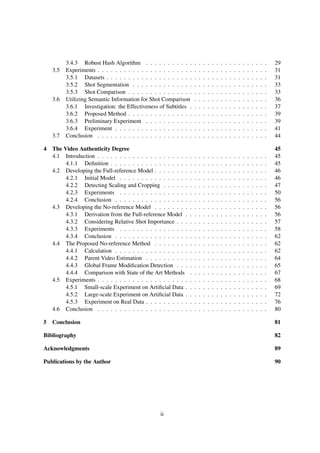
Figure 1.1: A timeline of our research with respect to related research fields.
common quality degradations such as blurring [23]. Our motivation for introducing these algorithms
is as follows: editing a video requires recompressing the video signal, which is usually a lossy opera-
tion that causes a decrease in visual quality [24]. Since the edited videos were created by editing the
parent video, the parent will have a higher visual quality than any of the edited videos created from it.
Therefore, visual quality assessment is relevant to authenticity estimation. However, since the video
signals of the edited videos can differ significantly due to the editing operations, directly applying the
algorithms to compare the visual quality of the edited videos is difficult [25].
Figure 1.1 shows a timeline of our research with respect to the related research fields.
1.2 Our Contribution
This thesis proposes a method that identifies the most authentic video by estimating the proportion
of information remaining from the parent video, even if the parent is not available. We refer to
this measure as the “authenticity degree”. The novelty of this proposed method consists of four
parts: (a) in the absence of the parent video, we estimate its content by comparing edited copies
of it; (b) we reduce the difference between the video signals of edited videos before performing a
3](https://image.slidesharecdn.com/da2f6a49-ec42-4092-b879-3c6b0720afd5-150824093659-lva1-app6891/85/main-6-320.jpg)
![Digital
Forensics
Digital
Forensics
Shot
Segmentation
Shot
Segmentation
Video
Similarity
Video
Similarity
Visual Quality
Assessment
Visual Quality
Assessment
Our ResearchOur Research
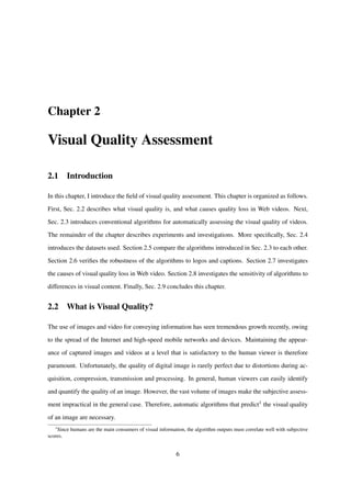
Figure 1.2: A map of research fields that are related to video authenticity.
visual quality comparison, thereby enabling the application of conventional NRQA algorithms; (c) we
collaboratively utilize the outputs of the NRQA algorithms to determine the visual quality of the parent
video; and (d) we enable the comparison of NRQA algorithm outputs for visually different shots.
Finally, since the proposed method is capable of detecting shot removal, scaling, and recompression,
it is effective for identifying the most authentic edited video. To the best of our knowledge, we are the
first to apply conventional NRQA algorithms to videos that have significantly different signals, and
the first to utilize video quality to determine the authenticity of a video. The proposed method has
applications in video retrieval: for example, it can be used to sort search results by their authenticity.
The effectiveness of our proposed method is demonstrated by experiments on real and artificial data.
In order to clarify our contribution, Figure 1.2 shows a map of research fields related to video
authenticity and the relationships between them. Each rectangle corresponds to a research field. The
closest related fields to the research proposed in this thesis are quality assessment and digital forensics.
To the best of our knowledge, these areas were unrelated until fairly recently, when it was proposed
that no-reference image quality assessment metrics be used to detect image forgery [26]. Furthermore,
the direct connection between video similarity and digital forensics was also made recently, when it
was proposed to use video similarity algorithms to recover the parent video from a set of edited
videos [20]. Our contribution is thus further bridging the gap between the visual quality assessment
and digital forensics by utilizing techniques from video similarity and shot segmentation. We are
looking forward to seeing new and interesting contributions.
4](https://image.slidesharecdn.com/da2f6a49-ec42-4092-b879-3c6b0720afd5-150824093659-lva1-app6891/85/main-7-320.jpg)
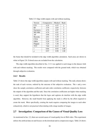
![1.3 Thesis Structure
This thesis consists of 5 chapters.
Chapter 2 reviews the field of quality assessment in greater detail, with a focus on conventional
methods for no-reference visual quality assessment. The chapter reviews several conventional NRQA
algorithms and compares their performance empirically. These algorithms enable the method pro-
posed in this thesis to quantify information loss. Finally, it demonstrates the limitations of existing
algorithms when applied to videos of differing visual content.
Chapter 3 proposes shot identification, an important pre-processing step for the method proposed
in this thesis. Shot identification enables the proposed method to:
1. Estimate the parent video from edited videos,
2. Detect removed shots, and
3. Apply the algorithms from Chapter 2.
The chapter first introduces algorithms for practical and automatic shot identification, and evaluates
their effectiveness empirically. Finally, the chapter introduces the shot identification algorithm and
evaluates its effectiveness as a whole.
Chapter 4 describes the proposed method for estimating the video authenticity. It offers a formal
definition of “video authenticity” and the development of several models for determining the authen-
ticity of edited videos in both full-reference and no-reference scenarios, culminating in a detailed
description of the method we recently proposed [27]. The effectiveness of the proposed method is
verified through a large volume of experiments on both artificial and real-world data.
Finally, Chapter 5 concludes the thesis and discusses potential future work.
5](https://image.slidesharecdn.com/da2f6a49-ec42-4092-b879-3c6b0720afd5-150824093659-lva1-app6891/85/main-8-320.jpg)
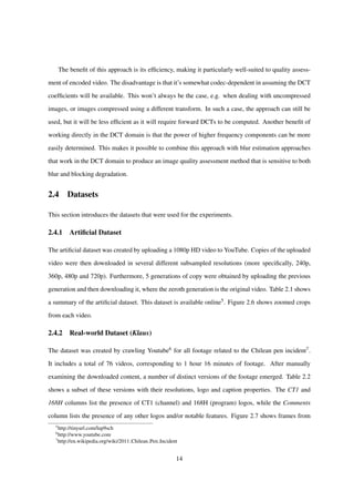
![There are many applications for visual quality assessment algorithms. First, they can be used to
monitor visual quality in an image acquisition system, maximizing the quality of the image that is
acquired. Second, they can be used for benchmarking existing image processing algorithms, such as,
for example, compression, restoration and denoising.
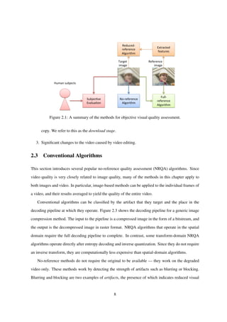
There are three main categories of objective visual quality assessment algorithms: full-reference,
reduced-reference, and no-reference. They are discussed in greater detail below. Figure 2.1 shows
a summary of the methods. While the figure describes images, the concepts apply equally well to
videos.
The full-reference category assumes that an image of perfect quality (the reference image) is
available, and assesses the quality of the target image by comparing it to the reference [25, 28–30].
While full-reference algorithms correlate well with subjective scores, there are many cases were the
reference image is not available.
Reduced-reference algorithms do not require the reference image to be available [31]. Instead,
certain features are extracted from the reference image, and used by the algorithm to assess the quality
of the target image. While such algorithms are more practical than full-reference algorithms, they still
require auxiliary information, which is not available in many cases.
No-reference algorithms2 assess the visual quality of the target image without any additional infor-
mation [23,32–37]. This thesis focuses on no-reference algorithms, since they are the most practical.
In the absence of the reference image, these algorithms attempt to identify and quantify the strength
of common quality degradations3. The remainder of this chapter focuses specifically on no-reference
algorithms, since they are most practical.
Finally, in the context of videos shared on the Web, there are several causes for decreases in visual
quality:
1. Recompression caused by repetitively downloading a video and uploading the downloaded
copy. This happens frequently and is known as reposting. We refer to this as the recompression
stage.
2. Downloading the video at lower than maximum quality and then uploading the downloaded
2
Also known as “blind” algorithms
3
Also known as “artifacts”
7](https://image.slidesharecdn.com/da2f6a49-ec42-4092-b879-3c6b0720afd5-150824093659-lva1-app6891/85/main-10-320.jpg)
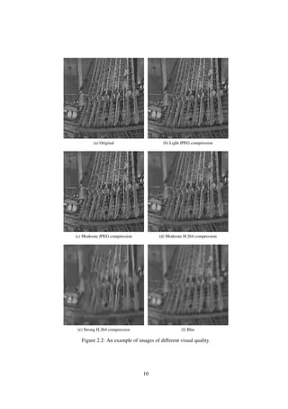
![quality. Blurring occurs when high-frequency spatial information is lost. This can be caused by strong
compression – since high-frequency transform coefficients are already weak in natural images, strong
compression can quantize them to zero. The loss of high-frequency spatial information can also be
caused by downsampling, as a consequence of the sampling theorem [38].
Blocking is another common artifact in images and video. It occurs as a result of too coarse a
quantization during image compression. It is often found in smooth areas, as those areas have weak
high frequency components that are likely to be set to zero as a result of the quantization process.
There are other known artifacts, such as ringing and mosquito noise, but they are not as common
in Web video. Therefore, the remainder of this chapter will focus on the blurring and blocking artifacts
only.
For example, Fig. 2.2(a) shows an original image of relatively high visual quality. Figures 2.2 (b)
to (f) show images of degraded visual quality due to compression and other operations.
2.3.1 Edge Width Algorithm
The conventional method [34] takes advantage of the fact that blurring causes edges to appear wider.
Sharp images thus have a narrower edge width than blurred images. The edge width in an image is
simple to measure: first, vertical edges are detected using the Sobel filter. Then, at each edge position,
the location of the local row minima and extrema are calculated. The distance between the extrema is
the edge width at that location.
One limitation of this algorithm is that it cannot be used to directly compare the visual quality of
two images of different resolutions, since the edge width depends on resolution. A potential work-
around for this limitation is to scale the images to a common resolution prior to comparison.
2.3.2 No-reference Block-based Blur Detection
While the edge width algorithm described in Section 2.3.1 is effective, it is computationally expensive
due to the edge detection step. Avoiding edge detection would allow the algorithm to be applied to
video more efficiently. The no-reference block-based blur detection (NR-BBD) algorithm [36] targets
video compressed in the H.264/AVC format [39], which includes an in-loop deblocking filter that
blurs macroblock boundaries to reduce the blocking artifact. Since the effect of the deblocking filter
is proportional to the strength of the compression, it is possible to estimate the amount of blurring
9](https://image.slidesharecdn.com/da2f6a49-ec42-4092-b879-3c6b0720afd5-150824093659-lva1-app6891/85/main-12-320.jpg)
![Entropy
decoding
Inverse
quan4za4on
Inverse
Transform
Spa4al-‐
domain
Algorithm
Forward
Transform
Transform-‐
domain
Algorithm
Transform-‐
domain
algorithm
Decompressed
image
011011101...
Compressed
image
Figure 2.3: Quality assessment algorithms at different stages of the decoding pipeline.
caused by the H.264/AVC compression by measuring the edge width at these macroblock boundaries.
Since this algorithm requires macroblock boundaries to be at fixed locations, it is only applicable to
video keyframes (also known as I-frames), as for all other types of frames the macroblock boundaries
are not fixed due to motion compensation.
2.3.3 Generalized Block Impairment Metric
The Generalized Block Impairment Metric (GBIM) [32] is a simple and popular spatial-domain
method for detecting the strength of the blocking artifact. It processes each scanline individually and
measures the mean squared difference across block boundaries. GBIM assumes that block boundaries
are at fixed locations. The weight at each location is determined by local luminance and standard
deviation, in an attempt to include the spatial and contrast masking phenomena into the model. While
this method produces satisfactory results, it has a tendency to misinterpret real edges that lie near
block boundaries.
As this is a spatial domain method, it is trivial to apply it to any image sequence. In the case of
video, full decoding of each frame will need to complete prior to applying the method. This method
corresponds to the blue block in Figure 2.3. Since this algorithm requires macroblock boundaries to
be at fixed locations, it is only applicable to video keyframes (also known as I-frames), as for all other
types of frames the macroblock boundaries are not fixed due to motion compensation.
11](https://image.slidesharecdn.com/da2f6a49-ec42-4092-b879-3c6b0720afd5-150824093659-lva1-app6891/85/main-14-320.jpg)
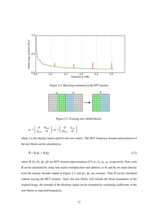
![2.3.4 Blocking Estimation in the FFT Domain
In [33], an FFT frequency domain approach is proposed to solve the false-positive problem of the
method introduced in Sec. 2.3.3. Because the blocking signal is periodic, it is more easily distin-
guished in the frequency domain. This approach models the degraded image as a non-blocky image
interfered with a pure blocky signal, and estimates the power of the blocky signal by examining the
coefficients for the frequencies at which blocking is expected to occur.
The method calculates a residual image and then applies a 1D FFT to each scanline of the residual
to obtain a collection of residual power spectra. This collection is then averaged to yield the com-
bined power spectrum. Figure 2.4 shows the combined power spectrum of the standard Lenna image
compressed at approximately 0.5311 bits per pixel. N represents the width of the FFT window, and
the x-axis origin corresponds to DC. The red peak at 0.125N is caused by blocking artifacts, as the
blocking signal frequency is 0.125 = 1
8 cycles per pixel4. The peaks appearing at 0.25N, 0.375N,
0.5N are all multiples of the blocking signal frequency and thus are harmonics.
This approach corresponds to the green blocks in Figure 2.3. It can be seen that it requires an
inverse DCT and FFT to be performed. This increases the complexity of the method, and is its main
disadvantage. The application of this method to video would be performed in similar fashion as
suggested for [32].
2.3.5 Blocking Estimation in the DCT Domain
In an attempt to provide a blocking estimation method with reduced computational complexity, [40]
proposes an approach that works directly in the DCT frequency domain. That is, the approach does not
require the full decoding of JPEG images, short-cutting the image decoding pipeline. This approach
is represented by the red block in Figure 2.3.
The approach works by hypothetically combining adjacent spatial blocks to form new shifted
blocks, as illustrated in Figure 2.5. The resulting block ˆb contains the block boundary between the
two original blocks b1 and b2.
Mathematically, this could be represented by the following spatial domain equation:
ˆb = b1q1 + b2q2 (2.1)
4
Block width for JPEG is 8 pixels
12](https://image.slidesharecdn.com/da2f6a49-ec42-4092-b879-3c6b0720afd5-150824093659-lva1-app6891/85/main-15-320.jpg)
![Table 2.6: Download stage visual quality degradation.
Resolution SSIM
1080p 1.00
780p 0.96
480p 0.92
360p 0.87
240p 0.81
Table 2.7: Recompression stage visual quality degradation.
Generation SSIM
0 1.00
1 0.95
2 0.94
3 0.93
4 0.92
5 0.91
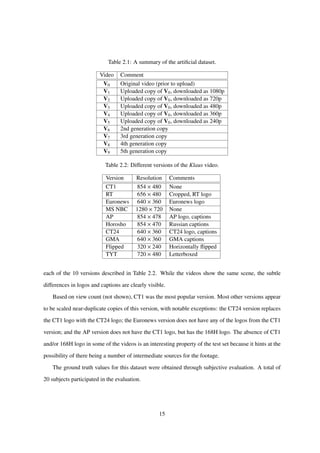
the SSIM output for each downloaded resolution of V0. Furthermore, Table 2.7 shows the SSIM
output for each copy generation. These tables allow the effect of each stage on the visual quality to
be compared. For example, downloading a 480p copy of a 1080p video accounts for as much quality
loss as downloading a 4th generation copy of the same 1080p video.
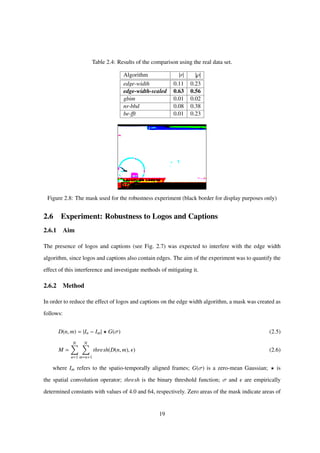
2.8 Investigation: Sensitivity to Visual Content
Visual content is known to affect NRQA algorithms in general and the edge width algorithm in par-
ticular [23]. To illustrate this effect, Fig. 2.9 shows images of similar visual quality, yet significantly
different edge widths: 2.92, 2.90, 3.92 and 4.68 for Figs. 2.9 (a), (b), (c) and (d), respectively. Without
normalization, the images of Figs. 2.9(c) and (d) would be penalized more heavily than the images of
Figs. 2.9(a) and (b). However, since these images are all uncompressed, they are free of compression
degradations, and there is no information loss with respect to the parent video. Therefore, the images
should be penalized equally, that is, not at all. Normalization thus reduces the effect of visual content
on the NRQA algorithm and achieves a fairer penalty function.
21](https://image.slidesharecdn.com/da2f6a49-ec42-4092-b879-3c6b0720afd5-150824093659-lva1-app6891/85/main-24-320.jpg)
![Chapter 3
Shot Identification
3.1 Introduction
This chapter introduces shot identification, an important pre-processing step that enables the method
proposed in this thesis. This chapter is organized as follows. Section 3.2 introduces the notation and
some initial definitions. Sections 3.3 and 3.4 describe algorithms for automatic shot segmentation
and comparison, respectively. Section 3.5 presents experiments for evaluating the effectiveness of the
algorithms presented in this chapter, and discusses the results. Section 3.6 investigates the application
of subtitles to shot identification, as described in one of our papers [6]. Finally, Sec. 3.7 concludes the
chapter.
3.2 Preliminaries
This section provides initial definitions and introduces the notation used in the remainder of the thesis.
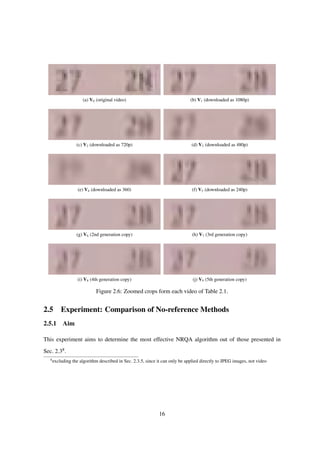
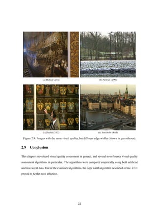
First, Fig. 3.1 shows that a single video can be composed of several shots, where a shot is a continuous
sequence of frames captured by a single camera. The figure shows one video, six shots, and several
hundred frames (only the first and last frame of each shot is shown).
Next, borrowing some notation and terminology from existing literature [20], we define the parent
video V0 as a video that contains some new information that is unavailable in other videos. The parent
video consists of several shots V1
0, V2
0, . . . , V
NV0
0 , where a shot is defined as a continuous sequence
of frames that were captured by the same camera over a particular period of time. The top part of
Fig. 3.2 shows a parent video that consists of NV0 = 4 shots. The dashed vertical lines indicate shot
boundaries. The horizontal axis shows time.
23](https://image.slidesharecdn.com/da2f6a49-ec42-4092-b879-3c6b0720afd5-150824093659-lva1-app6891/85/main-26-320.jpg)
![𝑉0
𝑉0
1
𝑉0
2
𝑉0
3
𝑉0
4
𝑡
Figure 3.2: An example of a parent video and its constituent shots.
𝑉1
𝑉2
𝑉3
𝑉1
1
≃ 𝑉0
2
𝑉1
2
≃ 𝑉0
3 𝑉1
3
≃ 𝑉0
4
𝑉2
1
≃ 𝑉0
3 𝑉2
2
≃ 𝑉0
2
𝑉2
3
≃ 𝑉0
1
𝑉3
1
≃ 𝑉0
4
𝑉3
2
≃ 𝑉0
2
Figure 3.3: An example of videos created by editing the parent video of Fig. 3.2.
example, I1
1 = I2
3 = I2
2 = i1, I2
1 = I1
2 = i2, I3
1 = I1
3 = i3, I3
2 = i4 and i1 through to i4 are different
from each other. The color of each node indicates its connected component. The actual value of
the shot identifier assigned to each connected component and the order of assigning identifiers to the
connected components are irrelevant.
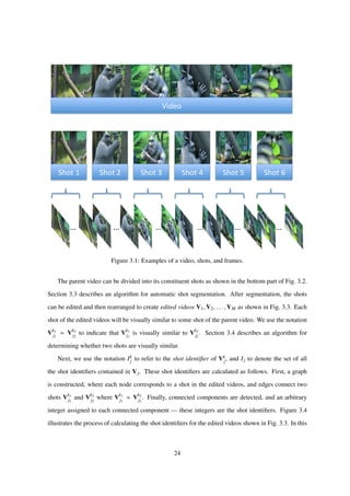
3.3 Shot Segmentation
Shot boundaries can be detected automatically by comparing the color histograms of adjacent frames,
and thresholding the difference [41]. More specifically, each frame is divided into 4 × 4 blocks, and a
64-bin color histogram is computed for each block. The difference between corresponding blocks is
then computed as:
F(f1, f2, r) =
63
x=0
{H(f1, r, x) − H(f2, r, x)}2
H(f1, r, x)
, (3.1)
25](https://image.slidesharecdn.com/da2f6a49-ec42-4092-b879-3c6b0720afd5-150824093659-lva1-app6891/85/main-28-320.jpg)
![𝑉1
1
𝑉1
2
𝑉1
3
𝑉3
1
𝑉3
2
𝑉2
1
𝑉2
2
𝑉2
3
Figure 3.4: An example of calculating the shot identifiers for the edited videos in Fig. 3.3.
where f1 and f2 are the two frames being compared; r is an integer corresponding to one of the 16
blocks; and H(f1, r, x) and H(f2, r, x) correspond to the xth bin of the color histogram of the rth block
of f1 and f2, respectively. The difference between the two frames is calculated as:
E(f1, f2) = SumOfMin
8 of 16, r=1 to 16
F(f1, f2, r), (3.2)
where the SumOfMin operator computes Eq. (3.1) for 16 different values of r and sums the smallest
8 results, and is explained in further detail by its authors [41]. Given a threshold υ, if E(f1, f2) > υ for
any two adjacent frames, then those two frames lie on opposite sides of a shot boundary. Although this
method often fails to detect certain types of shot boundaries [42], it is simple, effective and sufficient
for the purposes of this paper.
3.4 Shot Comparison
Since the picture typically carries more information than the audio, the majority of video similarity
algorithms focus on the moving picture only. For example, [43,44] calculate an visual signature from
the HSV histograms of individual frames. Furthermore, [45] proposes a hierarchical approach using a
combination of computationally inexpensive global signatures and, only if necessary, local features to
detect similar videos in large collections. On the other hand, some similarity algorithms focus only on
the audio signal. For example, [46] examines the audio signal and calculates a fingerprint, which can
be used in video and audio information retrieval. Methods that focus on both the picture and the audio
also exist. Finally, there are also methods that utilize the semantic content of video. For example, [47]
examines the subtitles of videos to perform cross-lingual novelty detection of news videos. Lu et al.
26](https://image.slidesharecdn.com/da2f6a49-ec42-4092-b879-3c6b0720afd5-150824093659-lva1-app6891/85/main-29-320.jpg)
![provide a good survey of existing algorithms [48].
3.4.1 A Spatial Algorithm
This section introduces a conventional algorithm for comparing two images based on their color his-
tograms [49]. First, each image is converted into the HSV color space, divided into four quadrants,
and a color histogram is calculated for each quadrant. The radial dimension (saturation) is quantized
uniformly into 3.5 bins, with the half bin at the origin. The angular dimension (hue) is quantized into
18 uniform sectors. The quantization for the value dimension depends on the saturation value: for
colors with saturation is near zero, the value is finely quantized into uniform 16 bins to better dif-
ferentiate between grayscale colors; for colors with higher saturation, the value is coarsely quantized
into 3 uniform bins. Thus the color histogram for each quadrant consists of 178 bins, and the feature
vector for a single image consists of 178 × 4 = 712 features, where a feature corresponds to a single
bin.
Next, the l1 distance between two images f1 and f2 is defined as follows:
l1(f1, f2) =
4
r=1
178
x=1
H(f1, r, x) − H(f2, r, x), (3.3)
where r refers to one of the 4 quadrants, and H(·, r, x) corresponds to the xth bin of the color histogram
for the rth quadrant. In order to apply Eq. (3.3) to shots, the simplest method is to apply it to the first
frames of the shots being compared, giving the following definition of visual similarity:
Vk1
j1
Vk2
j2
⇐⇒ l1(fk1
j1
, fk2
j2
) < φ, (3.4)
where τ is an empirically determined threshold; fk1
j1
and fk2
j2
are the first frames of Vk1
j1
and Vk2
j2
, respec-
tively.
3.4.2 A Spatiotemporal Algorithm
This section introduces a simple conventional algorithm for comparing two videos [50]. The algorithm
calculates the distance based on two components: spatial and temporal. The distances between their
corresponding spatial and temporal components of the two videos are first are compared separately,
and combined using a weighted sum. Each component of the algorithm is described in detail below.
27](https://image.slidesharecdn.com/da2f6a49-ec42-4092-b879-3c6b0720afd5-150824093659-lva1-app6891/85/main-30-320.jpg)
![Figure 3.5: Visualizing the spatial component (from [50]).
The spatial component is based on image similarity methods and calculated for each frame of the
video individually. The algorithm first discards the color information, divides the frame into p × q
equally-sized blocks and calculates the average intensity for each block, where p and q are pre-defined
constants. Each block is numbered in raster order, from 1 to m, where the constant m = p×q represents
the total number of blocks per frame. The algorithm then sorts the blocks by the average intensity. The
spatial component for a single frame is then given by the sequence of the m block numbers, ordered by
the average intensity. Figure 3.5 (a), (b) and (c) visualizes a grayscale frame divided into 3×3 blocks,
calculated average intensity, and the order of each block, respectively. The entire spatial component
for the entire video is thus an m × n matrix, where n is the number of frames in the video.
The distance between two spatial components is then calculated as:
dS (S 1, S 2) =
1
Cn
m
j=1
n
k=1
|S 1[j, k] − S 2[j, k]| , (3.5)
where S 1 and S 2 are the spatial components being compared, S 1[j, k] corresponds to the jth block
of the kth frame of S 1, and C is an normalization constant that represents the maximum theoretical
distance between any two spatial components for a single frame.
The temporal component utilizes the differences in corresponding blocks of sequential frames. It
is a matrix of m × n elements, where each element T[ j, k] corresponds to:
δk
j =
1 if Vj[k] > Vj[k − 1]
0 if Vj[k] = Vj[k − 1]
−1 if otherwise
, (3.6)
where Vj[k] represents the average intensity of the jth block of the kth frame of the video V. Figure 3.6
illustrates the calculation of the temporal component. Each curve corresponds to a different j. The
28](https://image.slidesharecdn.com/da2f6a49-ec42-4092-b879-3c6b0720afd5-150824093659-lva1-app6891/85/main-31-320.jpg)
![Figure 3.6: Visualizing the temporal component (from [50]).
horizontal and vertical axes correspond to k and Vj[k], respectively.
Next, the distance between two temporal components is calculated as:
dT (T1, T2) =
1
C(n − 1)
m
j=1
n
k=2
|T1[j, k] − T2[j, k]| . (3.7)
The final distance between two shots is calculated as:
dS T (Vk1
j1
, Vk2
j2
) = αDS (S k1
j1
, S k2
j2
) + (1 − α)DT (Tk1
j1
, Tk2
j2
), (3.8)
where S k1
j1
and Tk1
j1
are the spatial and temporal components of Vk1
j1
, respectively, and α is an empirically-
determined weighting parameter.
Finally, the algorithm enables the following definition of visual similarity:
Vk1
j1
Vk2
j2
⇐⇒ DS T (Vk1
j1
, Vk2
j2
) < τ, (3.9)
where χ is an empirically determined threshold.
3.4.3 Robust Hash Algorithm
The robust hashing algorithm yields a 64-bit hash for each shot [51]. The benefits of this method are
low computational and space complexity. Furthermore, once the hashes have been calculated, access
29](https://image.slidesharecdn.com/da2f6a49-ec42-4092-b879-3c6b0720afd5-150824093659-lva1-app6891/85/main-32-320.jpg)
![Figure 3.7: Extracting the DCT coefficients (from [51]).
to the original video is not required, enabling the application of the method to Web video sharing
portals (e.g. as part of the processing performed when a video is uploaded to the portal). After the
videos have been segmented into shots, as shown in the bottom of Fig. 3.2, the hashing algorithm
can be directly applied to each shot. The algorithm consists of several stages: (a) preprocessing, (b)
spatiotemporal transform and (d) hash computation. Each stage is described in more detail below.
The processing step focuses on the luma component of the video. First, the luma is downsampled
temporally to 64 frames. Then, the luma is downsampled spatially to 32 × 32 pixels per frame.
The motivation for the preprocessing step is to reduce the effect of differences in format and post-
processing.
The spatiotemporal transform step first applies a Discrete Cosine Transform to the preprocessed
video, yielding 32 × 32 × 64 DCT coefficients. Next, this step extracts 4 × 4 × 4 lower frequency
coefficients, as shown in Fig. 3.7. The DC terms in each dimension are ignored.
The hash computation step converts the 4 × 4 × 4 extracted DCT coefficients to a binary hash as
follows. First, the step calculates the median of the extracted coefficients. Next, the step replaces each
coefficient by a 0 if it is less than the median, and by a 1 otherwise. The result is an sequence of 64
bits. This is the hash.
30](https://image.slidesharecdn.com/da2f6a49-ec42-4092-b879-3c6b0720afd5-150824093659-lva1-app6891/85/main-33-320.jpg)
![Table 3.1: Summary of the datasets used in the experiments.
Name Videos Total dur. Shots IDs
Bolt 68 4 h 42 min 1933 275
Kerry 5 0 h 47 min 103 24
Klaus 76 1 h 16 min 253 61
Lagos 8 0 h 6 min 79 17
Russell 18 2 h 50 min 1748 103
Total 175 9 h 41 min 4116 480
The calculated hashes enable shots to be compared using the Hamming distance:
D(Vk1
j1
, Vk2
j2
) =
64
b=1
hk1
j1
[b] ⊕ hk2
j2
[b], (3.10)
where Vk1
j1
and Vk2
j2
are the two shots being compared; hk1
j1
and hk2
j2
are their respective hashes, rep-
resented as sequences of 64 bits each; and ⊕ is the exclusive OR operator. Finally, thresholding the
Hamming distance enables the determination of whether two shots are visually similar:
Vk1
j1
Vk2
j2
⇐⇒ D(Vk1
j1
, Vk2
j2
) < τ, (3.11)
where τ is an empirically determined threshold between 1 and 63.
3.5 Experiments
This section presents the results of experiments that compare the effectiveness of the algorithms in-
troduced in this chapter. Section 3.5.1 introduces the datasets used in the experiments. Then, Sec-
tions 3.5.2 and 3.5.3 evaluate the algorithms implemented by Equations (3.1) and (3.11), respectively.
3.5.1 Datasets
Table 3.1 shows the datasets used in the experiment, where each dataset consists of several edited
videos collected from YouTube. The “Shots” and “IDs” columns show the total number of shots and
unique shot identifiers, respectively. The Klaus dataset was first introduced in detail in Sec. 2.4.2.
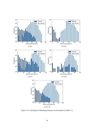
The remaining datasets were all collected in similar fashion. Figures 3.8(a)–(d), (e)–(h), (i)–(l), (m)–
(p), and (q)–(t) show a small subset of screenshots of videos from the Bolt, Kerry, Klaus, Lagos and
Russell datasets, respectively. The ground truth for each dataset was obtained by manual processing.
31](https://image.slidesharecdn.com/da2f6a49-ec42-4092-b879-3c6b0720afd5-150824093659-lva1-app6891/85/main-34-320.jpg)

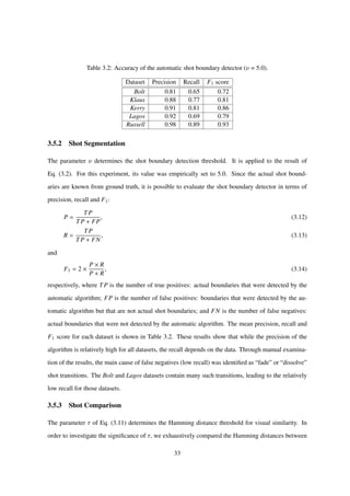
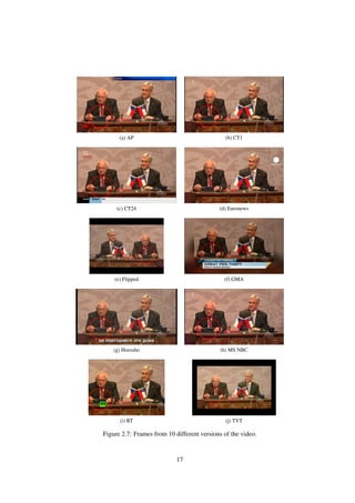
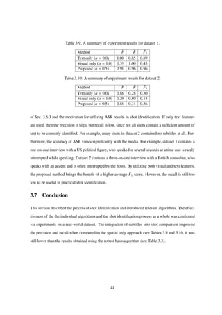
![Table 3.3: Accuracy of the automatic shot identifier function.
Dataset Precision Recall F1 score
Bolt 0.99 0.92 0.94
Kerry 1.00 1.00 1.00
Klaus 1.00 0.84 0.87
Lagos 1.00 0.62 0.71
Russell 1.00 0.98 0.98
then calculated.
Finally, Fig. 3.10 shows the F1 score for each dataset for different values of τ. From this figure, we
set the value of τ to 14 in the remainder of the experiment, as that value achieves the highest average F1
score across all the datasets. Table 3.3 shows the obtained results for that value of τ. From this table, it
is obvious that some datasets are easier to calculate shot identifiers for than others: for example, Kerry;
and some are more difficult: for example, Lagos. More specifically, in the Lagos case, the recall is
particularly low. This is because the dataset consists of videos that have been edited significantly,
for example, by inserting logos, captions and subtitles. In such cases, the hashing algorithm used is
not robust enough, and yields significantly different hashes for shots that a human would judge to be
visually similar. Nevertheless, Table 3.3 shows that automatic shot identifier calculation is possible.
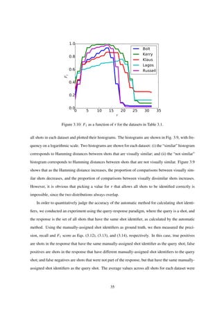
3.6 Utilizing Semantic Information for Shot Comparison
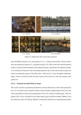
Web video often contains shots with little temporal activity, and shots that depict the same object at
various points in time. An example of such shots includes anchor shots and shots of people speaking
(see Figure 3.11). Since the difference in spatial and temporal content is low, the algorithms introduced
in Sections 3.4.1 and 3.4.2 cannot compare such shots effectively. However, if such shots contain
different speech, then they are semantically different. This section investigates the use of semantic
information for shot comparison. More specifically, the investigation will examine using subtitles to
distinguish visually similar shots.
There are several formats for subtitles [52]. In general, subtitles consist of phrases. Each phrase
consists of the actual text as well as the time period during which the text should be displayed. The
subtitles are thus synchronized with both the moving picture and the audio signal. Figure 3.12 shows
an example of a single phrase. The first row contains the phrase number. The second row contains
36](https://image.slidesharecdn.com/da2f6a49-ec42-4092-b879-3c6b0720afd5-150824093659-lva1-app6891/85/main-39-320.jpg)
![(a) Shot 3 (b) Shot 6 (c) Shot 9 (d) Shot 13 (e) Shot 15
(f) Shot 17 (g) Shot 19 (h) Shot 21 (i) Shot 25 (j) Shot 27
Figure 3.11: Unique shots from the largest cluster (first frames only).
2
00:00:03,000 −− > 00:00:06,000
Secretary of State John Kerry.
Thank you for joining us, Mr. Secretary.
Figure 3.12: An example of a phrase.
the time period. The remaining rows contain the actual text. In practice, the subtitles can be cre-
ated manually. Since this is a tedious process, Automatic Speech Recognition (ASR) algorithms that
extract the subtitles from the audio signal have been researched for over two decades [53]. Further-
more, research to extract even higher-level semantic information from the subtitles, such as speaker
identification [54], is also ongoing.
Subtitles are also useful for other applications. For example, [55] implements a video retrieval
system that utilizes the moving picture, audio signal and subtitles to identify certain types of scenes,
such as gun shots or screaming.
3.6.1 Investigation: the Effectiveness of Subtitles
This section introduces a preliminary investigation that confirms the limitations of the algorithm in-
troduced in Sec. 3.4.1 and demonstrates that subtitle text can help overcome these limitations. This
section first describes the media used in the investigation, before illustrating the limitations and a
potential solution.
37](https://image.slidesharecdn.com/da2f6a49-ec42-4092-b879-3c6b0720afd5-150824093659-lva1-app6891/85/main-40-320.jpg)
![Table 3.4: Subtitle text for each shot in the largest cluster.
Shot Duration Text
3 4.57 And I’m just wondering, did you...
6 30.76 that the President was about...
9 51.55 Well, George, in a sense, we’re...
13 59.33 the President of the United...
15 15.75 and, George, we are not going to...
17 84.38 I think the more he stands up...
19 52.39 We are obviously looking hard...
21 83.78 Well, I would, we’ve offered our...
25 66.50 Well, I’ve talked to John McCain...
27 66.23 This is not Iraq, this is not...
The video used in the investigation is an interview with a political figure, obtained from YouTube.
The interview lasts 11:30 and consists of 28 semantically unique shots. Shot segmentation was per-
formed manually. The average shot length was 24.61s. Since the video did not originally have subti-
tles, the subtitles were created manually.
Next, the similarity between the shots was calculated exhaustively using a conventional method [44],
and a clustering algorithm applied to the results. Since the shots are semantically unique, ideally, there
should be 28 singleton clusters – one cluster per shot. However, there were a total of 5 clusters as a
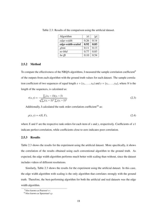
result of the clustering. Figure 3.13 shows the first frames from representative shots in each cluster.
The clusters are numbered arbitrarily. The representative shots were also selected arbitrarily. The
numbers in parentheses show the number of shots contained in each cluster. This demonstrates the
limitation of the conventional method, which focuses on the moving picture only.
Finally, Table 3.4 shows the subtitle text for each of the shots contained in the largest cluster, which
are shown in Fig. 3.11. The shot number corresponds to the ordinal number of the shot within the
original video. The table clearly shows that the text is significantly different for each shot. Including
the text in the visual comparison will thus overcome the limitations of methods that focus on the
moving picture only. In this investigation, since the subtitles were created manually, they are an
accurate representation of the speech in the video, and strict string comparisons are sufficient for shot
identification. If the subtitles are inaccurate (out of sync or poorly recognized words), then a more
tolerant comparison method will need to be used.
38](https://image.slidesharecdn.com/da2f6a49-ec42-4092-b879-3c6b0720afd5-150824093659-lva1-app6891/85/main-41-320.jpg)
![(a) C1 (4) (b) C2 (10) (c) C3 (7) (d) C4 (2) (e) C5 (1)
Figure 3.13: Representative shots from each cluster. The parentheses show the number of shots in
each cluster.
3.6.2 Proposed Method
The proposed method compares two video shots, Si and S j. The shots may be from the same video
or different videos. Each shot consists of a set of frames F(·) and a set of words W(·), corresponding
to the frames and subtitles contained by the shot, respectively. The method calculates the difference
between the two shots using a weighted average:
D(Si, S j) = αDf (Fi, Fj) + (1 − α)Dw(Wi, Wj), (3.15)
where α is a weight parameter, Df calculates the visual difference, and Dw calculates the textual dif-
ference. The visual difference can be calculated using any of the visual similarity methods mentioned
in Sec. 3.4. The textual difference can be calculated as the bag-of-words distance [56] commonly used
in information retrieval:
Dw(Wi, Wj) =
Wi ∩ Wj
Wi ∪ Wj
, (3.16)
where |·| calculates the cardinality of a set.
Equation 3.15 thus compares two shots based on their visual and semantic similarity.
3.6.3 Preliminary Experiment
This section describes an experiment that was performed to verify the effectiveness of the proposed
method. This section first reviews the purpose of the experiment, introduces the media used, describes
the empirical method and evaluation criteria and, finally, discusses the results.
The authenticity degree method introduced in Chapter 4 requires shots to be identified with high
precision and recall. The shot identification component must be robust to changes in visual quality,
39](https://image.slidesharecdn.com/da2f6a49-ec42-4092-b879-3c6b0720afd5-150824093659-lva1-app6891/85/main-42-320.jpg)
![Table 3.5: Video parameters
Video Fmt. Resolution Duration Shots
V1 MP4 1280 × 720 01:27 6
V2 MP4 1280 × 720 11:29 23
V3 FLV 640 × 360 11:29 23
V4 MP4 1280 × 720 11:29 23
V5 FLV 854 × 480 11:29 23
Table 3.6: ASR output example for one shot
Well, I, I would, uh, we’ve offered our friends, we’ve offered the Russians previously...
well highland and we’ve austerity our friendly the hovering the russians have previously...
highland and we’ve austerity our friendly the hovering the russians have previously...
well highland and we poverty our friendly pondered the russians have previously...
well highland and we’ve austerity our friendly the hovered russians have previously...
yet sensitive to changes in visual and semantic content. The aim of this experiment is thus to compare
shots that differ in the above parameters using the method proposed in Section 3.6.2 and determine
the precision and recall of the method.
The media used for the method includes five videos of a 11min 29s interview with a political
figure. All videos were downloaded from YouTube1. The videos differ in duration, resolution, video
and audio quality. None of the videos contained subtitles. Table 3.5 shows the various parameters
of each video, including the container format, resolution, duration and number of shots. During
pre-processing, the videos were segmented into shots using a conventional method [41]. Since this
method is not effective for certain shot transitions such as fade and dissolve, the results were cor-
rected manually. The subtitles for each shot were then created automatically using an open-source
automatic speech recognition library2. Table 3.6 shows an example of extracted subtitles, with a com-
parison to manual subtitles (top line). As can be seen from the table, the automatically extracted
subtitles differ from the manually extracted subtitles significantly. However, these differences appear
to be systematic. For example, “offered” is mis-transcribed as “hovering” in all of the four automatic
cases. Therefore, while the automatically extracted subtitles may not be useful for understanding the
semantic content of the video, they may be useful for identification.
The experiment first compared shots to each other exhaustively and manually, using a binary scale:
1
www.youtube.com
2
http://cmusphinx.sourceforge.net/
40](https://image.slidesharecdn.com/da2f6a49-ec42-4092-b879-3c6b0720afd5-150824093659-lva1-app6891/85/main-43-320.jpg)
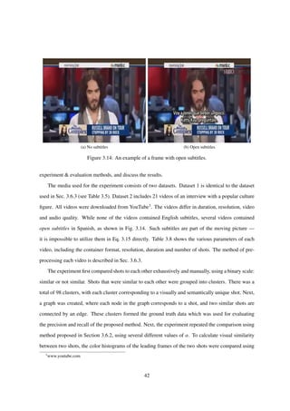
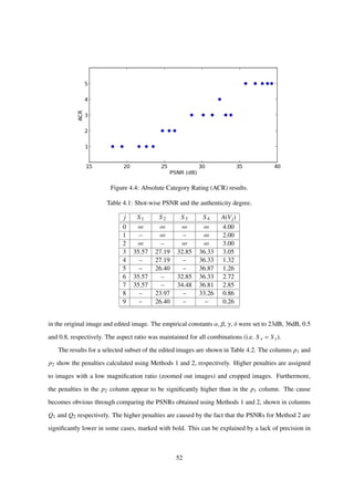
![Table 3.7: A summary of experiment results.
Method P R F1
Visual only 0.37 1.00 0.44
Proposed 0.98 0.96 0.96
similar or not similar. Shots that were similar to each other were grouped into clusters. There was a
total of 23 clusters, with each cluster corresponding to a visually and semantically unique shot. Each
node in the graph corresponds to a shot, and two similar shots are connected by an edge. These clusters
formed the ground truth data which was used for evaluating the precision and recall of the proposed
method. Next, the experiment repeated the comparison using method proposed in Section 3.6.2, using
an α of 0.5 to weigh visual and word differences equally. To calculate visual similarity between two
shots, the color histograms of the leading frames of the two shots were compared using a conventional
method [49].
To evaluate the effectiveness of the proposed method, the experiment measured the precision
and recall within a query-response paradigm. The precision, recall and F1 score were calculated as
Eqs. 3.12, 3.13 and 3.14. Within the query-response paradigm, the query was a single shot, selected
arbitrarily, and the response was all shots that were judged similar by the proposed method. True
positives were response shots that were similar to the query shot, according to the ground truth. False
positives were response shots that were not similar to the query shot, according to the ground truth.
False negatives were shots not in the response that were similar to the query shot, according to the
ground truth. The above set-up was repeated, using each of the shots as a query.
The average precision, recall and F-score were 0.98, 0.96, 0.96, respectively. In contrast, using
only visual features (α = 1.0) yields precision, recall and F-score of 0.37, 1.00, 0.44, respectively.
The results are summarized in Table 3.7. These results illustrate that the proposed method is effective
for distinguishing between shots that are visually similar yet semantically different.
3.6.4 Experiment
This section describes the new experiment. The purpose and method of performing the experiment
are identical to those of Sec. 3.6.3; differences with that experiment include a new dataset and a
new method of reporting the results. The following paragraphs describe the media used, review the
41](https://image.slidesharecdn.com/da2f6a49-ec42-4092-b879-3c6b0720afd5-150824093659-lva1-app6891/85/main-44-320.jpg)
![Table 3.8: Video parameters for dataset 2.
Video Fmt. Resolution Duration Shots
V1 MP4 636 × 358 01:00.52 15
V2 MP4 596 × 336 08:33.68 96
V3 MP4 640 × 360 08:23.84 93
V4 MP4 640 × 358 15:09.17 101
V5 MP4 1280 × 720 15:46.83 103
V6 MP4 640 × 360 08:42.04 97
V7 MP4 1280 × 720 06:26.99 8
V8 MP4 1280 × 720 09:19.39 97
V9 MP4 1280 × 720 08:59.71 99
V10 MP4 596 × 336 08:33.68 96
V11 MP4 596 × 336 08:33.68 96
V12 MP4 596 × 336 08:33.68 96
V13 MP4 596 × 336 08:33.68 96
V14 MP4 596 × 336 08:33.68 96
V15 MP4 596 × 336 08:33.61 97
V16 MP4 596 × 336 08:33.68 96
V17 MP4 1280 × 720 09:06.45 99
V18 MP4 634 × 350 00:10.00 1
V19 MP4 480 × 320 08:33.76 96
V20 MP4 596 × 336 08:33.68 96
V21 MP4 596 × 336 08:33.72 97
a conventional method [49].
To evaluate the effectiveness of the proposed method, the experiment measured the precision
and recall within a query-response paradigm. The precision, recall and F1 score were calculated as
Eqs. 3.12, 3.13 and 3.14. Within the query-response paradigm, the query was a single shot, selected
arbitrarily, and the response was all shots that were judged similar by the proposed method. True
positives were response shots that were similar to the query shot, according to the ground truth. False
positives were response shots that were not similar to the query shot, according to the ground truth.
False negatives were shots not in the response that were similar to the query shot, according to the
ground truth. The above set-up was repeated, using each of the shots as a query.
Tables 3.9 and 3.10 show the results for datasets 1 and 2, respectively. These results, in particular
those of Table 3.10 demonstrate the trade-off in utilizing both text and visual features for shot identi-
fication. If only visual features are used, then recall is high, but precision is low, since it is impossible
to distinguish between shots that are visually similar but semantically different — this was the focus
43](https://image.slidesharecdn.com/da2f6a49-ec42-4092-b879-3c6b0720afd5-150824093659-lva1-app6891/85/main-46-320.jpg)
![Chapter 4
The Video Authenticity Degree
4.1 Introduction
This chapter proposes the video authenticity degree and a method for its estimation. We begin the
proposal with a formal definition in Sec. 4.1.1 and the development of a full-reference model for the
authenticity degree in Sec. 4.2. Through experiments, we show that it is possible to determine the
authenticity of a video in a full-reference scenario, where the parent video is available. Next, Sec-
tion 4.3 describes the extension of the full-reference model to a no-reference scenario, as described
in another of our papers [3]. Through experiments, we verify that the model applies to a no-reference
scenario, where the parent video is unavailable. Finally, Section 4.4 proposes our final method for es-
timating the authenticity degree of a video in a no-reference scenario. Section 4.5 empirically verifies
the effectiveness of the method proposed in Sec. 4.4. The experiments demonstrate the effectiveness
of the method on real and artificial data for a wide range of videos. Finally, Section 4.6 concludes the
chapter.
4.1.1 Definition
The authenticity degree of an edited video Vj is defined as the proportion of remaining information
from its parent video V0. It is a positive real number between 0 and 1, with higher values correspond-
ing to high authenticity1.
1
Our earlier models did not normalize the authenticity degree to the range [0, 1].
45](https://image.slidesharecdn.com/da2f6a49-ec42-4092-b879-3c6b0720afd5-150824093659-lva1-app6891/85/main-48-320.jpg)
![4.2 Developing the Full-reference Model
4.2.1 Initial Model
In the proposed full-reference model, the parent video V0 is represented as a set of shot identifiers
S i (i = 1, . . . , N, where N is the number of shots in V0). For the sake of brevity, the shot with the
identifier equal to S i is referred to as “the shot S i” in the remainder of this section. Let the authenticity
degree of V0 be equal to N. V0 can be edited by several operations, including: (1) shot removal and (2)
video recompression, to yield a near-duplicate video Vj (j = 1, . . . , M, where M is the number of all
near-duplicates of V0). Since editing a video decreases its similarity with the parent, the authenticity
degree of Vj must be lower than that of V0. To model this, each editing operation is associated with a
positive penalty, as discussed below.
Each shot in the video conveys an amount of information. If a shot is removed to produce a near-
duplicate video Vj, then some information is lost, and the similarity between Vj and V0 decreases.
According to the definition of Section 4.1.1, the penalty for removing a shot should thus be pro-
portional to the amount of information lost. Accurately quantifying this amount requires semantic
understanding of the entire video. Since this is difficult, an alternative approach is to assume that all
the N shots convey identical amounts of information. Based on this assumption, the shot removal
penalty p1 is given by:
p1(V0, Vj, Si) =
1 if S i ∈ V0 ∧ S i Vj
0 otherwise
. (4.1)
Recompressing a video can cause a loss of detail due to quantization, which is another form of
information loss. The amount of information loss is proportional to the loss of detail. An objective
way to approximate the loss of detail is to examine the decrease in video quality. In a full-reference
scenario, one of the simplest methods to estimate the decrease in video quality is by calculating the
mean PSNR (peak signal-to-noise ratio) [24] between the compressed video and its parent. A high
PSNR indicates high quality; a low PSNR indicates low quality. While PSNR is known to have
limitations when comparing videos with different visual content [25], it is sufficient for our purposes
46](https://image.slidesharecdn.com/da2f6a49-ec42-4092-b879-3c6b0720afd5-150824093659-lva1-app6891/85/main-49-320.jpg)
![Figure 4.1: Penalty p2 as a function of PSNR.
since the videos are nearly identical. Thus, the recompression penalty p2 is given by:
p2(V0, Vj, S i) =
0 if S i Vj
1 if Qij < α
0 if Qij > β
(β − Qij)/(β − α) otherwise
, (4.2)
where α is a low PSNR at which the shot S i can be considered as missing; β is a high PSNR at which
no subjective quality loss is perceived; and V0[i] and Vj[i] refer to the image samples of shot S i in
video V0 and Vj, respectively, and
Qij = PSNR(V0[S i], Vj[S i]). (4.3)
A significant loss in quality thus corresponds to a higher penalty, with the maximum penalty being 1.
This penalty function is visualized in Fig. 4.1.
Finally, A(Vj), the authenticity degree of Vj, is calculated as follows:
A(Vj) = N −
N
i=1
p1(V0, Vj, S i) + p2(V0, Vj, S i). (4.4)
Note that if V0 and Vj are identical, then A(Vj) = N, which is a maximum and is consistent with the
definition of the authenticity degree from Sec. 4.1.1.
4.2.2 Detecting Scaling and Cropping
Scaling and cropping are simple and common video editing operations. Scaling is commonly per-
formed to reduce the bitrate for viewing on a device with a smaller display, and to increase the appar-
47](https://image.slidesharecdn.com/da2f6a49-ec42-4092-b879-3c6b0720afd5-150824093659-lva1-app6891/85/main-50-320.jpg)
![ent resolution (supersampling) in order to obtain a better search result ranking. Cropping is performed
to purposefully remove unwanted areas of the frame. Since both operations are spatial, they can be
modeled using images, and the expansion to image sequences (i.e. video) is trivial. For the sake of
simplicity, this section deals with images only.
Scaling can be modeled by an affine transformation [57]:
x
y
1
=
S x 0 −Cx
0 S y −Cy
0 0 1
x
y
1
, (4.5)
where (x, y) and (x , y ) are pixel co-ordinates in the original and scaled images, respectively; S x and
S y are the scaling factors in the horizontal and vertical directions, respectively; Cx and Cy are both 0.
Since the resulting (x , y ) may be non-integer and sparse, interpolation needs to be performed after
the above affine transform is applied to every pixel of the original image. This interpolation causes
a loss of information. The amount of information lost depends on the scaling factors and the type of
interpolation used (e.g. nearest-neighbor, bilinear, bicubic).
Cropping an image from the origin can be modeled by a submatrix operation:
I = I[{1, 2, . . . , Y}, {1, 2, . . . , X}], (4.6)
where I and I are the cropped and original image, respectively; Y and X are the number of rows and
columns, respectively, in I . Cropping from an arbitrary location (Cx,Cy) can be modeled through
a shift by applying the affine transform in Eq. 4.5 (with both S x and S y set to 1) prior to applying
Eq. (4.6). Since this operation involves removing rows and columns from I, it causes a loss of infor-
mation. The amount of information lost is proportional to the number of rows and columns removed.
Since both scaling and cropping cause a loss of information, their presence must incur a penalty.
If I is an original image and I is the scaled/cropped image, then the loss of information due to scaling
can be objectively measured by scaling I back to the original resolution, cropping I if required, and
measuring the PSNR [24]:
Q = PSNR(J, J ), (4.7)
where J is I restored to the original resolution and J is a cropped version of I. Cropping I is
necessary since PSNR is very sensitive to image alignment. The penalty for scaling is thus included
48](https://image.slidesharecdn.com/da2f6a49-ec42-4092-b879-3c6b0720afd5-150824093659-lva1-app6891/85/main-51-320.jpg)
![Figure 4.2: Penalty p as a function of Q and C.
in the calculation of Eq. (4.7), together with the penalty for recompression. The loss of information
due to cropping is proportional to the frame area that was removed (or inversely proportional to the
area remaining).
To integrate the two penalties discussed above with the model introduced in Sec. 4.2.1, I pro-
pose to expand the previously-proposed one-dimensional linear shot-wise penalty function, shown in
Figure 4.1, to two dimensions:
p(I, I ) = max 0, min 1,
Q − β
α − β
+
C − δ
γ − δ
, (4.8)
where C is the proportion of the remaining frame area of I ; (α, β) and (γ, δ) are the limits for the
PSNR and proportion of the remaining frame, respectively. Eq. (4.8) outputs a real number between
0 and 1, with higher values returned for low PSNR or remaining frame proportion. The proposed
penalty function is visualized in Fig. 4.2.
Implementing Eqs. (4.7) and (4.8) is trivial if the coefficients used for the original affine transform
in Eq. (4.5) are known. If they are unknown, they can be estimated directly from I and I in a full-
reference scenario. Specifically, the proposed method detects keypoints in each frame and calculates
their descriptors [58]. It then attempts to match the descriptors in one frame to the descriptors in the
49](https://image.slidesharecdn.com/da2f6a49-ec42-4092-b879-3c6b0720afd5-150824093659-lva1-app6891/85/main-52-320.jpg)
![other frame using the RANSAC algorithm [59]. The relative positions of the descriptors in each frame
allow an affine transform to be calculated. The remaining crop area is is calculated directly from the
coefficients of the affine transform. Furthermore, the coefficients of this affine transform allow the
remaining crop area to be calculated as:
C
j
i =
wj × hj
w0 × h0
, (4.9)
where (wj, hj) correspond to the dimensions of the keyframe from the near duplicate, after applying
the affine transform; and (w0, h0) correspond to the dimensions of the keyframe from the parent video.
4.2.3 Experiments
4.2.3.1 Testing the Initial Model
This section introduces an experiment that demonstrates the validity of model proposed in Sec. 4.2.1.
It consists of three parts: (1) selecting the model parameters; (2) creation of artificial test media; and
(3) discussion of the results.
The values for the model parameters α and β were determined empirically. First, the shields test
video (848 × 480 pixels, 252 frames) was compressed at various constant bitrates to produce near-
duplicate copies. A single observer then evaluated each of the near-duplicates on a scale of 1–5, using
the Absolute Category Rating (ACR) system introduced in ITU-T Recommendation P.910. The results
of the evaluation, shown in Fig. 4.4, demonstrate that the observer rated all videos with a PSNR lower
than approximately 23dB as 1 (poor), and all videos with a PSNR higher than approximately 36dB as
5 (excellent). The parameters α and β are thus set to 23 and 36, respectively.
To create the test set, first the single-shot test videos mobcal, parkrun, shields and stockholm
(848 × 480 pixels, 252 frames each) were joined, forming V0. These shots are manually assigned
unique signatures S 1, S 2, S 3 and S 4, respectively. Next, 9 near-duplicate videos Vj (j = 1, . . . , 9)
were created by repetitively performing the operations described in Sec. 4.2.1. For video compression,
constant-bitrate H.264/AVC compression was used, with two bitrate settings: high (512Kb/s) and low
(256Kb/s).
The results of the experiment are shown in Table 4.1. Each row of the table corresponds to a video
in the test set, with j = 0 corresponding to the parent video. The columns labeled S i (i = 1, 2, 3, 4)
50](https://image.slidesharecdn.com/da2f6a49-ec42-4092-b879-3c6b0720afd5-150824093659-lva1-app6891/85/main-53-320.jpg)
![Table 4.2: Results of the experiment.
S A1 A2 Q1 Q2 p1 p2
0.7 0.7 0.70 29.80 28.40 0.81 0.92
0.7 0.9 0.90 31.57 25.67 0.01 0.47
0.8 0.6 0.60 32.72 28.10 0.92 1.00
0.8 0.7 0.70 33.20 29.62 0.55 0.83
0.8 0.8 0.80 31.27 30.00 0.36 0.46
0.8 0.9 0.90 33.02 30.21 0.00 0.11
0.9 0.6 0.60 31.84 31.21 0.99 1.00
0.9 0.7 0.70 31.32 30.67 0.69 0.75
0.9 0.8 0.80 35.23 31.63 0.06 0.33
1.1 0.5 0.50 37.99 31.75 0.85 1.00
1.1 0.6 0.60 36.94 29.40 0.59 1.00
1.1 0.7 0.70 38.91 32.15 0.11 0.62
1.1 0.8 0.80 35.28 28.29 0.06 0.59
1.1 1.0 1.00 40.64 26.70 0.00 0.05
1.2 0.6 0.60 41.70 31.42 0.23 1.00
1.2 0.7 0.70 34.46 29.65 0.45 0.82
1.2 0.8 0.80 39.17 29.57 0.00 0.49
1.2 0.9 0.90 42.05 29.92 0.00 0.13
1.3 0.5 0.50 40.42 23.07 0.66 1.00
1.3 0.8 0.78 34.12 17.56 0.14 1.00
1.3 0.9 0.90 42.40 30.02 0.00 0.13
1.3 1.0 1.00 45.14 27.25 0.00 0.01
estimating the affine transform coefficients. PSNR is well-known to be very sensitive to differences
in image alignment. Using an alternative full-reference algorithm such as SSIM [29] may address this
discrepancy.
Finally, columns A1 and A2 show the proportion of the frame area remaining after cropping, cal-
culated using Methods 1 and 2, respectively. It is clear that the cropping area is being estimated
correctly. This will prove useful when performing scaling and cropping detection in a no-reference
scenario.
4.2.3.3 Testing the Extended Model on Videos
This section describes an experiment that was performed to evaluate the effectiveness of the proposed
method. In this experiment, human viewers were shown an parent video and near duplicates of the
parent. The viewers were asked to evaluate the similarity between the parent and each near duplicate.
The goal of the experiment was to compare these subjective evaluations to the output of the proposed
53](https://image.slidesharecdn.com/da2f6a49-ec42-4092-b879-3c6b0720afd5-150824093659-lva1-app6891/85/main-56-320.jpg)
![Table 4.3: Test set and test results for the Experiment of Sec. 4.2.3.3.
Video Editing Raw Norm. Prop.
V0 Parent video – – –
V1 3 shots removed 3.93 0.41 0.82
V2 7 shots removed 3.14 −0.47 0.50
V3 3/4 downsampling 4.93 1.41 0.90
V4 1/2 downsampling 3.93 0.48 0.85
V5 90% crop 3.93 0.47 0.32
V6 80% crop 2.57 −1.05 0.00
V7 Medium compression 3.14 −0.29 0.86
V8 Strong compression 2.42 −0.97 0.71
Table 4.4: Mean and standard deviations for each viewer.
Viewer µ σ
1 4.13 0.52
2 3.50 0.93
3 3.75 0.71
4 3.00 1.07
5 3.50 1.07
6 3.25 1.58
7 3.37 1.19
method. The details of the experiment, specifically, the data set, subjective experiment method, and
results, are described below.
The data set was created from a single YouTube news video (2min 50s, 1280 × 720 pixels). First,
shot boundaries were detected manually. There were a total of 61 shots, including transitions such
as cut, fade and dissolve [42]. Next, parts of the video corresponding to fade and dissolve transitions
were discarded, since they complicate shot removal. Furthermore, in order to reduce the burden on
the experiment subjects, the length of the video was reduced to 1min 20s by removing a small number
of shots at random. In the context of the experiment, this resulting video was the “parent video”.
This parent video had a total of 16 shots. Finally, near duplicates of the parent video were created by
editing it, specifically: removing shots at random, spatial downsampling (scaling), cropping, and com-
pression. Table 4.3 shows the editing operations that were performed to produce each near duplicate
in the “Editing” column.
During the experiment, human viewers were asked to evaluate the near duplicates: specifically, the
number of removed shots, visual quality, amount of cropping, and overall similarity with the parent,
54](https://image.slidesharecdn.com/da2f6a49-ec42-4092-b879-3c6b0720afd5-150824093659-lva1-app6891/85/main-57-320.jpg)
![Table 4.5: Rank-order of each near duplicate.
V1 V2 V3 V4 V5 V6 V7 V8
Subj. 4th 6th 1st 2nd 3rd 8th 5th 7th
Prop. 4th 6th 1st 3rd 7th 8th 2nd 5th
Table 4.6: Correlation with subjective results.
Method r ρ
Subjective 1.00 1.00
Objective 0.52 0.66
using a scale of 1 to 5. The viewers had access to the parent video. Furthermore, to simplify the task
of detecting shot removal, the viewers were also provided with a list of shots for each video.
Table 4.4 shows the mean and standard deviation for each viewer. From this table, we can see
that each viewer interpreted the concept of “similarity with the parent” slightly differently, which is
expected in a subjective experiment. To allow the scores from each viewer to be compared, they need
to be normalized in order to remove this subjective bias. The results are shown in Table 4.3, where the
“Raw” column shows the average score for each video, and the “Norm.” column shows the normalized
score, which is calculated by accounting for the mean and standard deviation for each individual
viewer (from Table 4.4). The “Prop.” column shows the authenticity degree that was calculated by the
proposed method. Table 4.5 shows the near duplicates in order of decreasing normalized subjective
scores and the proposed method outputs, respectively. From these results, we can see that for the
subjective and objective scores correspond for the top 4 videos. For the remaining 4 videos, there
appears to be no connection between the subjective and objective scores. To quantify this relationship,
Table 4.6 shows the correlation and rank-order correlation between the normalized subjective scores
and the proposed method outputs, as was done in the previous seminars. The correlation is lower than
what was reported in previous experiments [4], before scaling and cropping detection were introduced.
The decrease in correlation could be caused by an excessive penalty on small amounts of cropping
in Eq. (4.21). This hypothesis is supported by Table 4.5, where the rank-order of V5, a slightly
cropped video, is significantly lower in the subjective case. On the other hand, the rank-orders for
V6, a moderately cropped video, correspond to each other. This result indicates that viewers tolerated
a slight amount of cropping, but noticed when cropping became moderate. On the other hand, the
55](https://image.slidesharecdn.com/da2f6a49-ec42-4092-b879-3c6b0720afd5-150824093659-lva1-app6891/85/main-58-320.jpg)
![different rank-orders of V7 indicate that the penalty on compression was insufficient. Capturing this
behavior may require subjective tuning of the parameters α, β, γ, δ and possibly moving away from
the linear combination model, for example, to a sigmoid model.
4.2.4 Conclusion
This section introduced several models for determining the authenticity degree of an edited video in
a full-reference scenario. While such models cannot be applied to most real-world scenarios, they
enable greater understanding of the authenticity degree and the underlying algorithms. Section 4.3
further expands these models to no-reference scenario, thus enabling their practical application.
4.3 Developing the No-reference Model
4.3.1 Derivation from the Full-reference Model
Since V0 is not available in practice, A(Vj) of Eq. (4.4) cannot be directly calculated, and must be
estimated instead.
First, in order to realize Eq. (4.4), the no-reference model utilizes the available Web video context,
which includes the number of views for each video, to estimate the structure of the parent video by
focusing on the most-viewed shots. The set of most-viewed shots V0 can be calculated as follows:
V0 = S i |
Vj,Si∈Vj
W(Vj)
Wtotal
≥ β , (4.10)
where β is a threshold for determining the minimum number of views for a shot, W(Vj) is the number
of times video Vj was viewed, and Wtotal is the total number of views for all the videos in the near-
duplicate collection.
Next, the method of estimating the shot-wise penalty p is described. First, N is estimated as N =
V0 , where |·| denotes the number of shots in a video. Next, an estimate of the penalty function p that
is based on the above assumptions is described. The relative degradation strength Qij (i = 1, . . . , M,
j = 1, . . . , N) is defined as:
Qij =
QNR(Vj[S i]) − µi
σi
, (4.11)
where µi and σi are normalization constants for the shot S i, representing the mean and standard
deviation, respectively; Vj[S i] refers to the image samples of shot S i in video Vj; and QNR is a
56](https://image.slidesharecdn.com/da2f6a49-ec42-4092-b879-3c6b0720afd5-150824093659-lva1-app6891/85/main-59-320.jpg)
![no-reference quality assessment algorithm. Such algorithms estimate the quality by measuring the
strength of degradations such as wide edges [34] and blocking [32]. The result is a positive real
number, which is lower for higher quality videos. The penalty for recompression can then be defined
as:
ˆq(Vj, S i) =
0 if Qij < −γ
1 if Qij > γ
Qij+γ
2γ otherwise
, (4.12)
where γ is a constant that determines the scope of acceptable quality loss. A significant loss in quality
of a most-viewed shot thus corresponds to a higher penalty ˆq, with the maximum penalty being 1.
Next, ˆp, the estimate of the shot-wise penalty function p, can thus be calculated as:
ˆp(Vj, S i) =
1 if S i Vj
ˆq(Vj, S i) otherwise
. (4.13)
Equation (4.13) thus penalizes missing most-viewed shots with the maximum penalty equal to 1. If the
shot is present, the penalty is a function of the relative degradation strength Qij. The penalty function
ˆp does not require access to the parent video V0, since the result of Eq. (4.10) and no-reference quality
assessment algorithms are utilized instead. Finally, A, the estimate of the authenticity degree A, can
be calculated as:
A(Vj) = N −
N
i=1
ˆp(Vj, S i). (4.14)
4.3.2 Considering Relative Shot Importance
The authenticity degree model proposed in Sec. 4.3.1 suffers from several weaknesses. For example,
it relies on several assumptions that are difficult to justify. One of the main assumptions is that all
shots contain the same amount of information. In general, this is not always true, since some shots
obviously contain more information than others.
This section proposes an improved authenticity degree model that does not require the above
assumption. The proposed method inherits the same strategy, but adds a weighting coefficient to each
shot identifier:
A(Vj) = 1 −
i∈ˆI0
wi pi(Vj)
i∈ˆI0
wi
, (4.15)
57](https://image.slidesharecdn.com/da2f6a49-ec42-4092-b879-3c6b0720afd5-150824093659-lva1-app6891/85/main-60-320.jpg)
![where wi is the weighting coefficient of the shot with shot identifier equal to i. The value of wi should
be proportional to the “importance” of the shot: since some shots are more important than others,
the loss of their information should have a greater impact on the authenticity degree. The proposed
method calculates wi as the duration of the shot, in seconds. In other words, the proposed method
assumes that longer shots contain more information. This assumption is consistent with existing work
in video summarization [60].
4.3.3 Experiments
4.3.3.1 Evaluating the No-Reference Model
This section describes an experiment that illustrates the effectiveness of the proposed method. The
aim of the experiment is to look for correlations between the full-reference model, no-reference model
and subjective ratings from human observers. First, the data used in the experiments are introduced.
Next, the method of performing the experiment is described. Finally, the results are presented and
discussed.
Two data sets were used in this experiment. First, the artificial set consists of the same 10 videos
described in Sec. 4.2.3.1. Second, the lagos test set consists of 9 near-duplicate videos that were
retrieved from YouTube and includes news coverage related to a recent world news event. The videos
are compressed with H.264/AVC, but have different resolutions and bitrates. The audio signal in each
of the video was muted.
Two methods were used to detect the strength of correlation between the results and ground truth.
The first method is the correlation of the raw scores with the ground truth scores2, which is calculated
as:
r(X, Y) =
n
i=1 (Xi − ¯X)(Yi − ¯Y)
n
i=1 (Xi − ¯X)2 n
i=1 (Yi − ¯Y)2
, (4.16)
where n is the number of videos in a test set; X = [X1, . . . , Xn] represents the ground truth; Y =
[Y1, . . . , Yn] represents the results of the algorithm being evaluated; and ¯X and ¯Y are the means of X
and Y, respectively.
2
Also known as Pearson’s r.
58](https://image.slidesharecdn.com/da2f6a49-ec42-4092-b879-3c6b0720afd5-150824093659-lva1-app6891/85/main-61-320.jpg)
![Table 4.7: Results for each video in the artificial test set.
j A A EW GBIM
0 4.00 3.28 2.31 1.18
1 2.00 1.67 2.28 1.18
2 3.00 2.43 2.33 1.18
3 3.05 1.43 2.52 1.20
4 1.32 0.87 2.50 1.20
5 1.26 0.76 2.54 1.20
6 2.72 0.95 2.53 1.19
7 2.85 1.08 2.51 1.19
8 0.86 0.16 2.70 1.21
9 0.26 0.36 2.58 1.21
Table 4.8: Quantitative experiment results.
(a) Artificial
Method |r| |ρ|
FR 1.00 1.00
Subjective 0.82 0.76
Proposed 0.83 0.89
EW 0.61 0.60
GBIM 0.80 0.74
— — —
(b) Lagos
Method |r| |ρ|
Subjective 1.00 1.00
Proposed 0.55 0.30
EW 0.40 0.25
GBIM 0.50 0.07
Views 0.03 0.12
Delay 0.40 0.15
The second method is the the correlation of the ranks of the raw scores with the ranks of the
ground truth scores3. First, the ranks of each element in X and Y are calculated to yield x and y. The
final output of the second method is:
ρ(X, Y) = r(x, y). (4.17)
For both r and ρ, a value of ±1 indicates strong correlation with the ground truth, and is therefore a
desirable result. A value of zero indicates poor correlation with the ground truth.
To perform the experiment, the proposed no-reference model was first applied to the data to ob-
tain an estimate of the authenticity degree for each video of the artificial set. The results are shown
in Table 4.7. The columns A and A show the actual and estimated authenticity degrees, respectively.
The columns EW and GBIM show the result of directly applying the no-reference quality assessment
algorithms of edge width [34] and blocking strength [32], respectively, to each video. From these
3
Also known as Spearman’s ρ.
59](https://image.slidesharecdn.com/da2f6a49-ec42-4092-b879-3c6b0720afd5-150824093659-lva1-app6891/85/main-62-320.jpg)
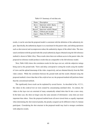
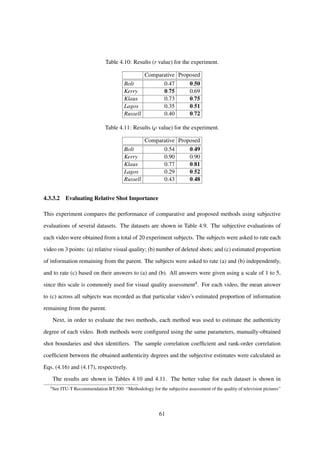
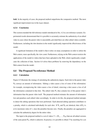
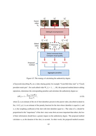
![that longer shots contain more information. This assumption is consistent with existing work in video
summarization [60].
Specifically, each pi(·) is calculated as:
pi(Vj) =
1 if i Ij
γgi(Vj) otherwise
, (4.19)
where the notation i Ij means “Vj doesn’t contain a shot with an identifier equal to i”; gi(Vj)
is the global frame modification penalty, described in detail in Sec. 4.4.3, for the shot of Vj whose
identifier is equal to i. The parameter γ determines the trade-off between information loss through
global frame modifications and information loss through shot removal. Since, in practice, global
frame modifications can never remove all the information in a shot entirely, γ should be a positive
value less than 1. Equation (4.19) thus assigns the maximum penalty for shot removal, and a fraction
of the maximum penalty for global frame modifications.
There may be significant differences between the edited videos: for example some shots may be
added/missing (e.g. Fig. 4.5). As demonstrated in Sec. 2.8, this prevents the effective application
of conventional NRQA algorithms, since the output of such algorithms will be influenced by the
added/missing shots. Before NRQA algorithms can be applied effectively, this influence must be
reduced. The proposed method achieves this in two ways. First, when calculating the global frame
modification penalty, the proposed method works on a shot ID basis, and only compares the raw visual
quality of shots that have the same shot identifier (common content). Second, the proposed method
prevents missing/added shots from affecting the outcome of NRQA algorithms. More specifically, if
a shot is added (not part of the estimated parent ˆI0), then it is ignored completely by Eq. (4.18). If a
shot is missing (part of the estimated parent), then a shot removal penalty is assigned by Eq. (4.19).
4.4.2 Parent Video Estimation
In order to detect shot removal, the proposed method first defines Bi as the number of edited videos
that contain a shot with an identifier equal to i. Then, ˆI0, the estimate of the set of shot identifiers
present in V0, is calculated as:
ˆI0 =
M
j=1
{i|i ∈ Ij,
Bi
M
> δ}, (4.20)
64](https://image.slidesharecdn.com/da2f6a49-ec42-4092-b879-3c6b0720afd5-150824093659-lva1-app6891/85/main-67-320.jpg)
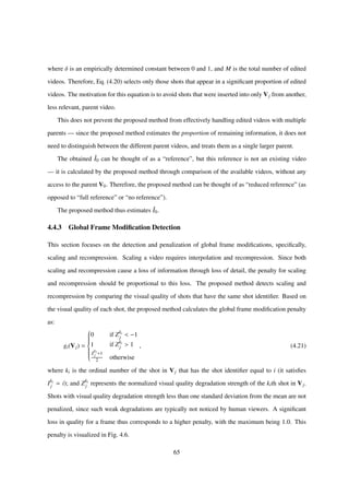
![1.5 1.0 0.5 0.0 0.5 1.0 1.5
Normalized degradation strength
0.2
0.0
0.2
0.4
0.6
0.8
1.0
1.2
Penalty
Figure 4.6: Global frame modification penalty p(·).
In order to calculate gi(Vki
j ), the proposed method first calculates Qki
j , the raw visual quality of Vki
j
as:
Qki
j = mean(QNR(Vki
j [l1]), . . . , QNR(Vki
j [lL])), (4.22)
where QNR is an NRQA algorithm that measures edge width [23]; and l1, . . . , lL are the frame numbers
of the intra-predicted frames (frames that are encoded independently of other frames [39], hereafter
referred to as “keyframes”) of the shot. The proposed method focuses only on the keyframes to reduce
computational complexity and speed up processing. The output of QNR corresponds to the strength of
visual quality degradations in the frame: a high value indicates low quality, and a low value indicates
high quality.
Next, since the strength of detected visual quality degradations depends on the actual content of
the frame, the raw visual quality is normalized as:
Zki
j =
Qki
j − µi
σi
, (4.23)
where µi and σi are normalization parameters for the shot whose identifier is equal to i, representing
the mean and standard deviation, respectively. The proposed method performs this normalization
to fairly penalize shots with different visual content, since visual content is known to affect NRQA
algorithms, as shown in Sec. 2.8.
66](https://image.slidesharecdn.com/da2f6a49-ec42-4092-b879-3c6b0720afd5-150824093659-lva1-app6891/85/main-69-320.jpg)
![The normalization step above is a novel component of the proposed method. Typically, the output
of an NRQA algorithm for a single image is not enough to qualitatively determine its visual quality. In
other words, without a reference value, it is impossible to judge whether the visual quality of the image
is good or bad. The normalization step provides the proposed method with a reference visual quality
level, thus enabling (a) the qualitative assessment of a shot’s visual quality; and (b) the comparison
of visual quality between shots with different content (see Fig. 2.9). The effect of normalization is
shown empirically in Table 4.14.
Finally, the result of Eq. (4.21) is a real number that is lower for higher quality videos. Therefore,
it is an effective penalty for recompressed and scaled videos. The proposed method thus detects and
penalizes recompression and scaling. While there are other editing operations, such as color trans-
formations, the addition of logos and subtitles, and spatial cropping, the proposed method does not
explicitly detect or penalize them. However, applying these editing operations requires recompressing
the video, which causes a decrease in visual quality. Since the proposed method explicitly focuses on
visual quality degradation, it will penalize the edited videos in proportion to the extent of the visual
quality degradation.
4.4.4 Comparison with State of the Art Methods
In theory, many of the conventional methods introduced in Chapter 1.1 could be used as comparative
methods, as they share the same general purpose as the proposed method. In practice, however, com-
paring the conventional methods to the proposed method directly is difficult. For example, forensic
methods are typically used to aid the judgement of an experienced human operator as opposed to
being applied automatically. Furthermore, they focus on determining whether individual videos have
been tampered or not, which is slightly different from the concrete problem the proposed method is
attempting to solve: comparing near-duplicate videos and determining which one is the closest to the
parent. For this reason, we do not compare our proposed method with any of the forensic methods.
Similarly, while the method for reconstructing the parent video from its near duplicates [20] is
very relevant to our work, it doesn’t achieve the same end result. More specifically, it can be used
as an alternative implementation of part of our proposed method: the shot identification function
described in Chapter 3 and the shot removal detector described in Sec. 4.4.2. Since it does not contain
67](https://image.slidesharecdn.com/da2f6a49-ec42-4092-b879-3c6b0720afd5-150824093659-lva1-app6891/85/main-70-320.jpg)
![V0
V1 V2 V3
V4 V8
V9
V5 V6 V7
Figure 4.7: The philogeny tree for the dataset of Table 4.12.
functionality to determine which of the edited videos is most similar to the parent video, it also cannot
be directly compared to our proposed method.
Similarly, video philogeny [19] could be used as a comparative method, with some modifications.
After the video philogeny tree is constructed, the root of the tree will be the parent video, and the
edited videos will be its descendants. Authenticity of a video could then be calculated to be inversely
proportionate to the depth of the corresponding node in the philogeny tree. However, there are some
limitations to this approach. For example, Fig. 4.7 shows the philogeny tree for the dataset of Ta-
ble 4.12. From the graph, it is obvious that V1, V2 and V3 would have the same authenticity degree,
since they are all at a depth of 1 in the tree. However, their expected authenticity degrees are different,
as explained by Table 4.12. This problem could be solved by improving the video philogeny method
to consider visual quality. We intend to address this in our future work.
4.5 Experiments
This section describes three experiments that were conducted to verify the effectiveness of the pro-
posed method. Section 4.5.1 evaluates the proposed method in a semi-controlled environment, using
a small amount of artificial data that is uploaded to YouTube5, with a known parent. Section 4.5.2
5
http://www.youtube.com
68](https://image.slidesharecdn.com/da2f6a49-ec42-4092-b879-3c6b0720afd5-150824093659-lva1-app6891/85/main-71-320.jpg)
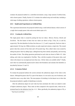
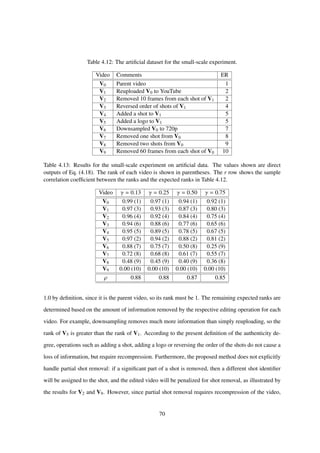
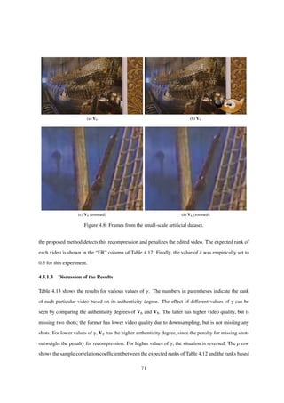
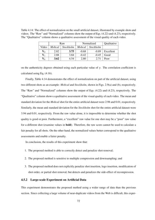
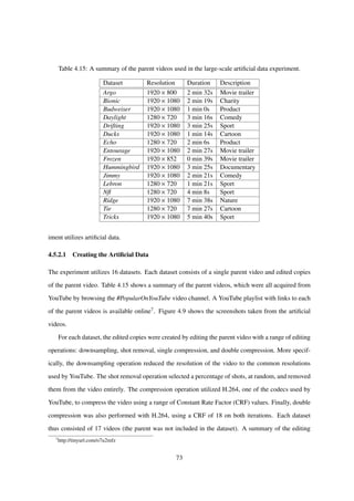
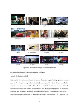
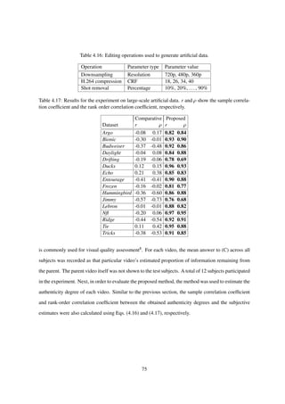
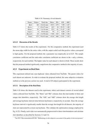
![4.5.3.2 Comparative Methods
For comparative methods, this experiment uses:
1. The number of views of each video,
2. The upload timestamp for each video,
3. The mean visual quality of each video, and
4. The proposed method with γ = 0 (consider shot removal only).
The number of views and upload timestamp are available from the metadata of each video. The
mean visual quality was obtained by calculating the mean edge width [23] for each individual frame,
as implemented by Eq. (4.22). Finally, the output of all methods was configured such that positive
values correspond to higher authenticity. Therefore, high correlation coefficients correspond to the
best methods.
4.5.3.3 Parameter Selection
The parameter γ determines the trade-off between penalizing shot removal and penalizing global
frame modifications. Figure 4.10 shows the effect of different values of γ on the results for each of the
each of the datasets in Table 4.18. From the figure, it is obvious that the optimal value of γ is different
for each dataset. We set γ = 0.7 in the remainder of the experiments.
The value for the parameter δ, which determines what proportion of edited videos must contain a
particular shot identifier in order for that identifier to be part of the parent video, was empirically set
to 0.1.
4.5.3.4 Discussion of the Results
Tables 4.19 and 4.20 show the sample correlation coefficient r and rank-order correlation coefficient
ρ, respectively. Each line corresponds to one of the datasets in Table 4.18. The number of asterisks
indicates the rank of the particular method within a specific dataset: , and indicate the
best, second best and third best methods, respectively. From the tables, the following observations
can be made:
77](https://image.slidesharecdn.com/da2f6a49-ec42-4092-b879-3c6b0720afd5-150824093659-lva1-app6891/85/main-80-320.jpg)
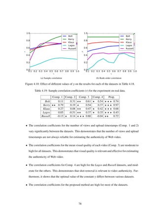
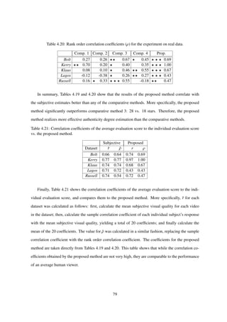
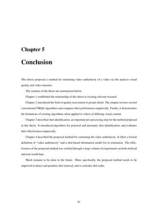
![Bibliography
[1] M. Penkov, T. Ogawa, and M. Haseyama, “Fidelity estimation of online video based on video
quality measurement and Web information,” in Proceedings of the 26th Signal Processing Sym-
posium, vol. A3-5, 2011, pp. pp. 70–74.
[2] ——, “A note on the application of Web information to near-duplicate online video detection,”
vol. 36, no. 9, pp. 201–205, 2012.
[3] ——, “A Study on a Novel Framework for Estimating the Authenticity Degree of Web Videos,”
in Digital Signal Processing Symposium, 2012.
[4] ——, “A Method for Estimating the Authenticity Degree of Web Videos and Its Evaluation,” in
International Workshop on Advanced Image Technology (IWAIT), 2013, pp. 534–538.
[5] ——, “Quantification of Video Authenticity by Considering Video Editing through Visual Qual-
ity Assessment,” in ITC-CSCC, 2013, pp. 838–841.
[6] ——, “A note on improving authenticity degree estimation through Automatic Speech Recogni-
tion,” ITE Technical Report, vol. 38, no. 7, pp. 341–346, 2014.
[7] ——, “Estimation of Video Authenticity through Collaborative Use of Available Video
Signals,” ITE Transactions on Media Technology and Applications, vol. 3, no. 3, pp. 214–225,
Jul. 2015. [Online]. Available: https://www.jstage.jst.go.jp/article/mta/3/3/3 214/ article
[8] R. D. Oliveira, M. Cherubini, and N. Oliver, “Looking at near-duplicate videos from a
human-centric perspective,” ACM Trans. Multimedia Comput. Commun. Appl., vol. 6, no. 3,
2010. [Online]. Available: http://portal.acm.org/citation.cfm?id=1823749
82](https://image.slidesharecdn.com/da2f6a49-ec42-4092-b879-3c6b0720afd5-150824093659-lva1-app6891/85/main-85-320.jpg)
![[9] X. Wu, C.-w. Ngo, and Q. Li, “Threading and autodocumenting news videos: a promising
solution to rapidly browse news topics,” IEEE Signal Processing Magazine, vol. 23, no. 2,
pp. 59–68, Mar. 2006. [Online]. Available: http://ieeexplore.ieee.org/xpl/articleDetails.jsp?
arnumber=1621449
[10] S. Siersdorfer, S. Chelaru, W. Nejdl, and J. S. Pedro, “How useful are your comments?:
analyzing and predicting youtube comments and comment ratings,” ser. WWW ’10. Raleigh,
North Carolina, USA: ACM, 2010, Conference proceedings (article), pp. 891–900. [Online].
Available: http://portal.acm.org/citation.cfm?id=1772690.1772781
[11] X. Wu, C.-W. Ngo, A. Hauptmann, and H.-K. Tan, “Real-Time Near-Duplicate Elimination for
Web Video Search With Content and Context,” Multimedia, IEEE Transactions on, vol. 11,
no. 2, pp. 196–207, Feb. 2009. [Online]. Available: http://ieeexplore.ieee.org/xpls/abs all.jsp?
arnumber=4757425
[12] D. Kundur and D. Hatzinakos, “Digital watermarking for telltale tamper proofing and
authentication,” Proceedings of the IEEE, vol. 87, no. 7, pp. 1167–1180, Jul. 1999. [Online].
Available: http://ieeexplore.ieee.org/lpdocs/epic03/wrapper.htm?arnumber=771070
[13] I. Cox, M. Miller, J. Bloom, J. Fridrich, and T. Kalker, “Digital Watermarking and
Steganography,” Nov. 2007. [Online]. Available: http://dl.acm.org/citation.cfm?id=1564551
[14] A. Piva, “An Overview on Image Forensics,” ISRN Signal Processing, vol. 2013, p. 22.
[15] S. Milani, M. Fontani, P. Bestagini, M. Barni, A. Piva, M. Tagliasacchi, and S. Tubaro,
“An overview on video forensics,” APSIPA Transactions on Signal and Information
Processing, vol. 1, p. e2, Aug. 2012. [Online]. Available: http://journals.cambridge.org/
abstract S2048770312000029
[16] S.-p. Li, Z. Han, Y.-z. Chen, B. Fu, C. Lu, and X. Yao, “Resampling forgery detection
in JPEG-compressed images,” vol. 3, Coll. of Software, Nankai Univ., Tianjin, China.
IEEE, Oct. 2010, Conference proceedings (article), pp. 1166–1170. [Online]. Available:
http://ieeexplore.ieee.org/xpls/abs all.jsp?arnumber=5646732
83](https://image.slidesharecdn.com/da2f6a49-ec42-4092-b879-3c6b0720afd5-150824093659-lva1-app6891/85/main-86-320.jpg)
![[17] G. Cao, Y. Zhao, R. Ni, L. Yu, and H. Tian, “Forensic detection of median
filtering in digital images,” Inst. of Inf. Sci., Beijing Jiaotong Univ., Beijing, China.
IEEE, Jul. 2010, Conference proceedings (article), pp. 89–94. [Online]. Available:
http://ieeexplore.ieee.org/xpls/abs all.jsp?arnumber=5583869
[18] A. Popescu and H. Farid, “Exposing digital forgeries by detecting traces of resampling,” Signal
Processing, IEEE Transactions on, vol. 53, no. 2, pp. 758–767, Feb. 2005. [Online]. Available:
http://ieeexplore.ieee.org/xpls/abs all.jsp?arnumber=1381775
[19] Z. Dias, A. Rocha, and S. Goldenstein, “Video Phylogeny: Recovering near-duplicate
video relationships,” in 2011 IEEE International Workshop on Information Forensics and
Security. IEEE, Nov. 2011, pp. 1–6. [Online]. Available: http://ieeexplore.ieee.org/lpdocs/
epic03/wrapper.htm?arnumber=6123127
[20] S. Lameri, P. Bestagini, A. Melloni, S. Milani, A. Rocha, M. Tagliasacchi, and S. Tubaro, “Who
is my parent? Reconstructing video sequences from partially matching shots,” in IEEE Interna-
tional Conference on Image Processing (ICIP), 2014.
[21] N. Diakopoulos and I. Essa, “Modulating video credibility via visualization of quality
evaluations,” in Proceedings of the 4th workshop on Information credibility - WICOW
’10. New York, New York, USA: ACM Press, Apr. 2010, p. 75. [Online]. Available:
http://dl.acm.org/citation.cfm?id=1772938.1772953
[22] A. K. Moorthy and A. C. Bovik, “Visual quality assessment algorithms: what does the
future hold?” Multimedia Tools Appl., vol. 51, no. 2, pp. 675–696, Jan. 2011. [Online].
Available: http://portal.acm.org/citation.cfm?id=1938166http://www.springerlink.com/content/
wmp6181r08757v39
[23] P. Marziliano, F. Dufaux, S. Winkler, and T. Ebrahimi, “A no-reference perceptual blur metric,”
in Proceedings of the International Conference on Image Processing. 2002. Proceedings. 2002
International Conference on, vol. 3, Genimedia SA, Lausanne, Switzerland. Toronto, Ont.,
Canada: IEEE, 2002, Conference proceedings (article), pp. III–57–III–60 vol.3. [Online].
Available: http://ieeexplore.ieee.org/xpls/abs all.jsp?arnumber=1038902
84](https://image.slidesharecdn.com/da2f6a49-ec42-4092-b879-3c6b0720afd5-150824093659-lva1-app6891/85/main-87-320.jpg)
![[24] Z. Wang and A. C. Bovik, “Modern Image Quality Assessment,” Synthesis Lectures on Image,
Video, and Multimedia Processing, vol. 2, no. 1, pp. 1–156, Jan. 2006. [Online]. Available:
http://www.morganclaypool.com/doi/abs/10.2200/S00010ED1V01Y200508IVM003
[25] Q. Huynh-Thu and M. Ghanbari, “Scope of validity of PSNR in image/video quality
assessment,” Electronics Letters, vol. 44, no. 13, p. 800, 2008. [Online]. Available:
http://digital-library.theiet.org/content/journals/10.1049/el 20080522
[26] F. Battisti, M. Carli, and A. Neri, “Image forgery detection by means of no-reference quality
metrics,” in SPIE Vol. 8303, 2012. [Online]. Available: http://spie.org/Publications/Proceedings/
Paper/10.1117/12.910778
[27] M. Penkov, T. Ogawa, and M. Haseyama, “Estimation of Video Authenticity through Collabora-
tive Use of Available Video Signals,” ITE Transactions on Media Technology and Applications,
2015.
[28] A. Bovik and J. Kouloheris, “Full-reference video quality assessment considering structural
distortion and no-reference quality evaluation of MPEG video,” in Proceedings. IEEE
International Conference on Multimedia and Expo, vol. 1. IEEE, 2002, pp. 61–64. [Online].
Available: http://ieeexplore.ieee.org/articleDetails.jsp?arnumber=1035718
[29] Z. Wang, A. Bovik, H. Sheikh, and E. Simoncelli, “Image quality assessment: from error
visibility to structural similarity,” IEEE Transactions on Image Processing, vol. 13, no. 4, pp.
600–612, Apr. 2004. [Online]. Available: http://ieeexplore.ieee.org/xpls/abs all.jsp?arnumber=
1284395
[30] S. Winkler and P. Mohandas, “The Evolution of Video Quality Measurement: From PSNR to
Hybrid Metrics,” IEEE Transactions on Broadcasting, vol. 54, no. 3, pp. 660–668, Sep. 2008.
[Online]. Available: http://ieeexplore.ieee.org/articleDetails.jsp?arnumber=4550731
[31] Q. Li and Z. Wang, “Reduced-Reference Image Quality Assessment Using Divisive
Normalization-Based Image Representation,” IEEE Journal of Selected Topics in Signal
Processing, vol. 3, no. 2, pp. 202–211, Apr. 2009. [Online]. Available: http://ieeexplore.ieee.
org/articleDetails.jsp?arnumber=4799311
85](https://image.slidesharecdn.com/da2f6a49-ec42-4092-b879-3c6b0720afd5-150824093659-lva1-app6891/85/main-88-320.jpg)
![[32] H. Wu and M. Yuen, “A generalized block-edge impairment metric for video coding,” Signal
Processing Letters, IEEE, vol. 4, no. 11, pp. 317–320, Nov. 1997. [Online]. Available:
http://ieeexplore.ieee.org/xpls/abs all.jsp?arnumber=641398
[33] Z. Wang, A. Bovik, and B. Evan, “Blind measurement of blocking artifacts in
images,” vol. 3, Dept. of Electr. & Comput. Eng., Texas Univ., Austin, TX. IEEE,
2000, Conference proceedings (article), pp. 981–984 vol.3. [Online]. Available: http:
//ieeexplore.ieee.org/xpls/abs all.jsp?arnumber=899622
[34] P. Marziliano, F. Dufaux, S. Winkler, and T. Ebrahimi, “Perceptual blur and ringing metrics:
Application to JPEG2000,” vol. 19, no. 2. Elsevier, Feb. 2004, Conference proceedings
(article), pp. 163–172. [Online]. Available: http://citeseerx.ist.psu.edu/viewdoc/summary?doi=
10.1.1.170.4680
[35] X. Zhu and P. Milanfar, “A no-reference sharpness metric sensitive to blur and noise,” 2009,
Conference proceedings (article). [Online]. Available: http://citeseerx.ist.psu.edu/viewdoc/
summary?doi=10.1.1.153.5611
[36] L. Debing, C. Zhibo, M. Huadong, X. Feng, and G. Xiaodong, “No Reference Block Based Blur
Detection,” Thomson Corp. Res., Beijing, China. IEEE, Jul. 2009, Conference proceedings
(article), pp. 75–80. [Online]. Available: http://ieeexplore.ieee.org/xpls/abs all.jsp?arnumber=
5246974
[37] Z. Wang and A. Bovik, “Reduced- and No-Reference Image Quality Assessment,” IEEE
Signal Processing Magazine, vol. 28, no. 6, pp. 29–40, Nov. 2011. [Online]. Available: http:
//ieeexplore.ieee.org/xpl/articleDetails.jsp?tp=&arnumber=6021882&contentType=Journals+
&+Magazines&searchWithin=no-reference&ranges=2011 2013 p Publication Year&
searchField=Search All&queryText=video+quality+assessment
[38] J. D. Gibson and A. Bovik, Eds., Handbook of Image and Video Processing, 1st ed. Academic
Press, Inc., 2000. [Online]. Available: http://portal.acm.org/citation.cfm?id=556230
[39] I. Richardson, The H.264 Advanced Video Compression Standard. John Wiley & Sons, 2010.
[Online]. Available: http://books.google.com/books?id=LJoDiPnBzQ8C
86](https://image.slidesharecdn.com/da2f6a49-ec42-4092-b879-3c6b0720afd5-150824093659-lva1-app6891/85/main-89-320.jpg)
![[40] S. Liu and A. Bovik, “Efficient DCT-domain blind measurement and reduction of blocking
artifacts,” Circuits and Systems for Video Technology, IEEE Transactions on, vol. 12, no. 12,
pp. 1139–1149, Dec. 2002. [Online]. Available: http://ieeexplore.ieee.org/xpls/abs all.jsp?
arnumber=1175450
[41] A. Nagasaka and Y. Tanaka, “Automatic Video Indexing and Full-Video Search for Object
Appearances.” North-Holland Publishing Co., 1992, Conference proceedings (article), pp.
113–127. [Online]. Available: http://portal.acm.org/citation.cfm?id=719786
[42] R. Lienhart, “Comparison of automatic shot boundary detection algorithms,” pp. 290–301,
1999. [Online]. Available: http://citeseerx.ist.psu.edu/viewdoc/summary?doi=10.1.1.87.9460
[43] S.-c. Cheung and A. Zakhor, “Efficient video similarity measurement
with video signature,” in Proceedings. International Conference on Im-
age Processing, vol. 1. IEEE, 2002, pp. I–621–I–624. [Online]. Avail-
able: http://ieeexplore.ieee.org/xpl/articleDetails.jsp?tp=&arnumber=1038101&contentType=
Conference+Publications&searchField=Search All&queryText=cheung+zakhor
[44] ——, “Fast similarity search and clustering of video sequences on the world-wide-
web,” IEEE Transactions on Multimedia, vol. 7, no. 3, pp. 524–537, Jun. 2005.
[Online]. Available: http://citeseerx.ist.psu.edu/viewdoc/summary?doi=10.1.1.67.3547http:
//ieeexplore.ieee.org/lpdocs/epic03/wrapper.htm?arnumber=1430728
[45] X. Wu, A. G. Hauptmann, and C. W. Ngo, “Practical elimination of near-duplicates from
web video search,” ser. MULTIMEDIA ’07. Augsburg, Germany: ACM, 2007, Conference
proceedings (article), pp. 218–227. [Online]. Available: http://portal.acm.org/citation.cfm?id=
1291280
[46] E. Wold, T. Blum, D. Keislar, and J. Wheaten, “Content-based classification, search, and
retrieval of audio,” IEEE Multimedia, vol. 3, no. 3, pp. 27–36, 1996. [Online]. Available:
http://ieeexplore.ieee.org/lpdocs/epic03/wrapper.htm?arnumber=556537
[47] X. Wu, A. G. Hauptmann, and C.-W. Ngo, “Novelty detection for cross-lingual news stories
with visual duplicates and speech transcripts,” in Proceedings of the 15th international
87](https://image.slidesharecdn.com/da2f6a49-ec42-4092-b879-3c6b0720afd5-150824093659-lva1-app6891/85/main-90-320.jpg)
![conference on Multimedia - MULTIMEDIA ’07. New York, New York, USA: ACM Press,
Sep. 2007, p. 168. [Online]. Available: http://dl.acm.org/citation.cfm?id=1291233.1291274
[48] J. Lu, “Video fingerprinting for copy identification: from research to industry applications,”
in IS&T/SPIE Electronic Imaging, E. J. Delp III, J. Dittmann, N. D. Memon, and
P. W. Wong, Eds., Feb. 2009, pp. 725 402–725 402–15. [Online]. Available: http:
//proceedings.spiedigitallibrary.org/proceeding.aspx?articleid=1335155
[49] S.-c. Cheung and A. Zakhor, “Efficient video similarity measurement with video signature,”
Circuits and Systems for Video Technology, IEEE Transactions on, vol. 13, no. 1, pp. 59–74,
Jan. 2003. [Online]. Available: http://ieeexplore.ieee.org/xpls/abs all.jsp?arnumber=1180382
[50] C. Kim and B. Vasudev, “Spatiotemporal sequence matching for efficient video copy detection,”
IEEE Transactions on Circuits and Systems for Video Technology, vol. 15, 2005. [Online].
Available: http://ieeexplore.ieee.org/xpls/abs all.jsp?arnumber=1377368
[51] B. Coskun, B. Sankur, and N. Memon, “Spatio-Temporal Transform Based Video Hashing,”
IEEE Transactions on Multimedia, vol. 8, no. 6, pp. 1190–1208, Dec. 2006. [Online]. Available:
http://ieeexplore.ieee.org/lpdocs/epic03/wrapper.htm?arnumber=4014210
[52] J. Tiedemann, “Building a Multilingual Parallel Subtitle Corpus,” in Computational Linguistics
in the Netherlands, 2007. [Online]. Available: http://citeseerx.ist.psu.edu/viewdoc/summary?
doi=10.1.1.148.6563
[53] R. A. Cole, J. Mariani, H. Uszkoreit, A. Zaenen, G. Varile, A. Zampolli, and V. Zue,
“Survey of the State of the Art in Human Language Technology.” [Online]. Available:
http://citeseerx.ist.psu.edu/viewdoc/summary?doi=10.1.1.50.7794
[54] M. Everingham, J. Sivic, and A. Zisserman, “Hello! My name is... Buffy –
automatic naming of characters in TV video,” Sep. 2006. [Online]. Available: http:
//eprints.pascal-network.org/archive/00002192/
[55] T. Langlois, T. Chambel, E. Oliveira, P. Carvalho, G. Marques, and A. Falc˜ao, “VIRUS,” in
Proceedings of the 14th International Academic MindTrek Conference on Envisioning Future
88](https://image.slidesharecdn.com/da2f6a49-ec42-4092-b879-3c6b0720afd5-150824093659-lva1-app6891/85/main-91-320.jpg)
![Media Environments - MindTrek ’10. New York, New York, USA: ACM Press, Oct. 2010, p.
197. [Online]. Available: http://dl.acm.org/citation.cfm?id=1930488.1930530
[56] C. D. Manning, P. Raghavan, and H. Schutze, Introduction to Information Retrieval. Cambridge
University Press, 2008. [Online]. Available: http://portal.acm.org/citation.cfm?id=1394399
[57] R. C. Gonzalez and R. E. Woods, Digital Image Processing (3rd Edition), 3rd ed. Prentice
Hall, Aug. 2007. [Online]. Available: http://www.amazon.com/exec/obidos/redirect?tag=
citeulike07-20&path=ASIN/013168728X
[58] D. Lowe, “Object recognition from local scale-invariant features,” in Proceedings of the Seventh
IEEE International Conference on Computer Vision. IEEE, 1999, pp. 1150–1157 vol.2.
[Online]. Available: http://ieeexplore.ieee.org/xpl/articleDetails.jsp?arnumber=790410
[59] M. A. Fischler and R. C. Bolles, “Random sample consensus: a paradigm for model
fitting with applications to image analysis and automated cartography,” Communications
of the ACM, vol. 24, no. 6, pp. 381–395, Jun. 1981. [Online]. Available: http:
//dl.acm.org/citation.cfm?id=358669.358692
[60] S. Uchihashi and J. Foote, “Summarizing video using a shot importance measure and a
frame-packing algorithm,” in 1999 IEEE International Conference on Acoustics, Speech, and
Signal Processing. Proceedings. ICASSP99 (Cat. No.99CH36258), vol. 6. IEEE, 1999, pp.
3041–3044 vol.6. [Online]. Available: http://ieeexplore.ieee.org/lpdocs/epic03/wrapper.htm?
arnumber=757482
89](https://image.slidesharecdn.com/da2f6a49-ec42-4092-b879-3c6b0720afd5-150824093659-lva1-app6891/85/main-92-320.jpg)

This doctoral thesis examines methods for estimating the authenticity of videos by analyzing their visual quality and structure. It aims to determine the proportion of information an edited video retains from its original parent video. The thesis first evaluates existing no-reference algorithms for visual quality assessment. It then explores techniques for shot segmentation and comparison. It also develops models for calculating a video's authenticity degree based on factors like visual quality, shot importance, and evidence of global modifications. The goal is to objectively estimate a video's authenticity when only the video itself is available for analysis, without relying on external metadata.