Downloaded 10 times


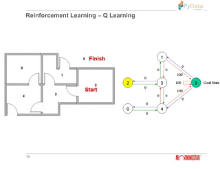
![Reinforcement Learning – Q Learning
17
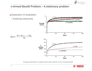
Q(state, action) = R(state, action) + Gamma * Max[Q(next state, all
actions)]
http://mnemstudio.org/path-finding-q-learning-tutorial.htm
Q(state, action) = R(state, action) + Gamma * Max[Q(next state, all actions)]](https://image.slidesharecdn.com/pydatareinforcementlearning-190421043127/85/Machine-learning-Vs-Deep-learning-Vs-Reinforcement-learning-Pydata-Mumbai-17-320.jpg)
![Reinforcement Learning – Q Learning
18
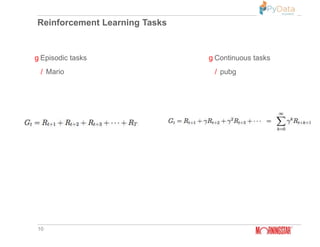
http://mnemstudio.org/path-finding-q-learning-tutorial.htm
Q(state, action) = R(state, action) + Gamma * Max[Q(next state, all actions)]](https://image.slidesharecdn.com/pydatareinforcementlearning-190421043127/85/Machine-learning-Vs-Deep-learning-Vs-Reinforcement-learning-Pydata-Mumbai-18-320.jpg)
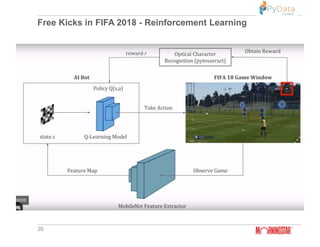
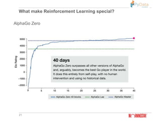

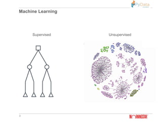
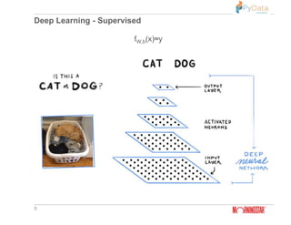
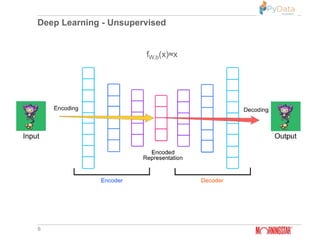
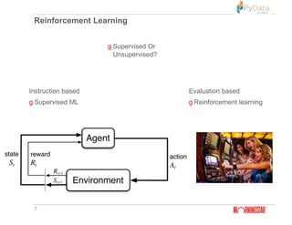
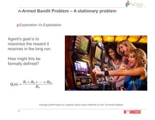
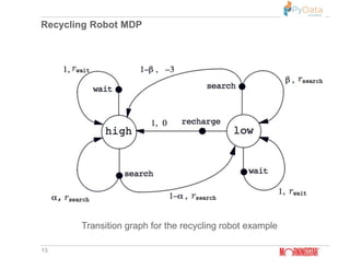
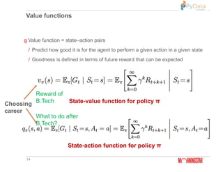
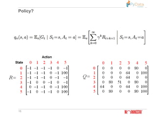
The document summarizes Pratik Bhavsar's presentation at the PyData Meetup 11 in Mumbai on August 11, 2018. The presentation covered the differences between machine learning, deep learning, and reinforcement learning. It provided examples of supervised and unsupervised deep learning and discussed the n-armed bandit problem and reinforcement learning tasks. Key concepts from reinforcement learning like the Markov property, value functions, Q-learning, and applications were also summarized. The presentation concluded with an example of using reinforcement learning for free kicks in the FIFA 2018 video game.