machine Learning subject of third year information technology unit 2.pptx
These are the Academic Presentation of Machine learning subject of Third Year Information Technology 2019 pattern of SPPU.
For the insem exam this is the second unit.
A linear classifieris achieved by making a classification decision depending on the value of a linear
combination of the characteristics.
An object’s characteristics can also be called feature values and are typically offered to the machine in a
vector known as a feature vector.
Such classifiers are suitable for practical problems like document classification and also for problems that
consist of many variables(features), to reach accuracy levels in comparison to non-linear classifiers despite of
taking less time to train and use.
A linear classifier classifies based on a decision on the value of linear combination of characteristics.
A particular class is defined by linear classifier that will merge into its weight with all characteristics.
E.g. merging of all samples of car together.
Linear Classification Model
3.
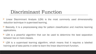
Linear DiscriminantAnalysis (LDA) is the most commonly used dimensionality
reduction technique in supervised learning.
Basically, it is a preprocessing step for pattern classification and machine learning
applications.
LDA is a powerful algorithm that can be used to determine the best separation
between two or more classes.
LDA is a supervised learning algorithm, which means that it requires a labelled
training set of data points in order to learn the linear discriminant function.
Discriminant Function
4.
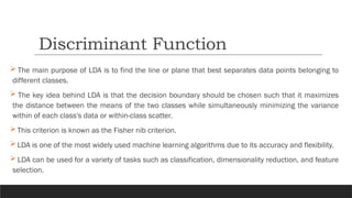
The mainpurpose of LDA is to find the line or plane that best separates data points belonging to
different classes.
The key idea behind LDA is that the decision boundary should be chosen such that it maximizes
the distance between the means of the two classes while simultaneously minimizing the variance
within of each class's data or within-class scatter.
This criterion is known as the Fisher nib criterion.
LDA is one of the most widely used machine learning algorithms due to its accuracy and flexibility.
LDA can be used for a variety of tasks such as classification, dimensionality reduction, and feature
selection.
Discriminant Function
5.
Discriminant Function
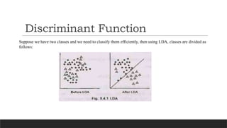
Suppose wehave two classes and we need to classify them efficiently, then using LDA, classes are divided as
follows:
6.
LDA algorithm worksbased on the following steps:
a) The first step is to calculate the means and standard deviation of each feature.
b) Within class scatter matrix and between class scatter matrix is calculated
c) These matrices are then used to calculate the eigenvectors and eigenvalues.
e) LDA uses this transformation matrix to transform the data into a new space with k
dimensions.
f) Once the transformation matrix transforms the data into new space with k dimensions,
LDA can then be used for classification or dimensionality -reduction
Discriminant Function
7.
Benefits ofusing LDA:
a) LDA is used for classification problems.
b) LDA is a powerful tool for dimensionality reduction.
c) LDA is not susceptible to the "curse of dimensionality" like many other machine
learning algorithms.
Discriminant Function
8.
Performance evaluationis the quantitative measure of how well a trained model performs on
specific model evaluation metrics in machine learning.
This information can then be used to determine if a model is ready to move onto the next
stage of testing, be deployed more broadly, or is in need of more training or retraining.
Two of the most important categories of evaluation methods are classification and regression
model performance metrics.
Understanding how these metrics are calculated will enable you to choose what is most
important within a given model, and provide quantitative measures of performance within that
metric.
Performance Evaluation
9.
Classification metricsare generally used for discrete values a model might produce when it has finished
classifying all the given data.
In order to clearly display the raw data needed to calculate desired classification metrics, a confusion matrix
for a model can be created.
The confusion matrix is a matrix used to determine the performance of the classification models for a given
set of test data.
It can only be determined if the true values for test data are known.
The matrix itself can be easily understood, but the related terminologies may be confusing.
Since it shows the errors in the model performance in the form of a matrix, hence also known as an error
matrix.
Confusion Matrix
10.
Some features ofConfusion matrix are given below:
For the 2 prediction classes of classifiers, the matrix is of 2*2 table, for 3 classes, it is 3*3
table, and so on.
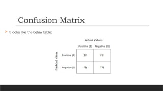
The matrix is divided into two dimensions, that are predicted values and actual values along
with the total number of predictions.
Predicted values are those values, which are predicted by the model, and actual values are the
true values for the given observations.
Confusion Matrix
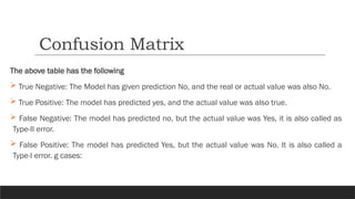
The above tablehas the following
True Negative: The Model has given prediction No, and the real or actual value was also No.
True Positive: The model has predicted yes, and the actual value was also true.
False Negative: The model has predicted no, but the actual value was Yes, it is also called as
Type-II error.
False Positive: The model has predicted Yes, but the actual value was No. It is also called a
Type-I error. g cases:
Confusion Matrix
13.
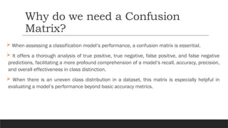
When assessinga classification model’s performance, a confusion matrix is essential.
It offers a thorough analysis of true positive, true negative, false positive, and false negative
predictions, facilitating a more profound comprehension of a model’s recall, accuracy, precision,
and overall effectiveness in class distinction.
When there is an uneven class distribution in a dataset, this matrix is especially helpful in
evaluating a model’s performance beyond basic accuracy metrics.
Why do we need a Confusion
Matrix?
14.
Accuracy
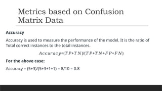
Accuracy is usedto measure the performance of the model. It is the ratio of
Total correct instances to the total instances.
𝐴𝑐𝑐𝑢𝑟𝑎𝑐𝑦=( + )/( + + + )
𝑇𝑃 𝑇𝑁 𝑇𝑃 𝑇𝑁 𝐹𝑃 𝐹𝑁
For the above case:
Accuracy = (5+3)/(5+3+1+1) = 8/10 = 0.8
Metrics based on Confusion
Matrix Data
15.
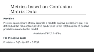
Precision
Precision is ameasure of how accurate a model’s positive predictions are. It is
defined as the ratio of true positive predictions to the total number of positive
predictions made by the model.
Precision= /( + )
𝑇𝑃 𝑇𝑃 𝐹𝑃
For the above case:
Precision = 5/(5+1) =5/6 = 0.8333
Metrics based on Confusion
Matrix Data
16.
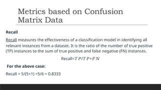
Recall
Recall measures theeffectiveness of a classification model in identifying all
relevant instances from a dataset. It is the ratio of the number of true positive
(TP) instances to the sum of true positive and false negative (FN) instances.
Recall= / +
𝑇𝑃 𝑇𝑃 𝐹𝑁
For the above case:
Recall = 5/(5+1) =5/6 = 0.8333
Metrics based on Confusion
Matrix Data
17.
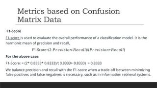
F1-Score
F1-score is usedto evaluate the overall performance of a classification model. It is the
harmonic mean of precision and recall,
F1-Score=(2 )/( +
)
⋅𝑃𝑟𝑒𝑐𝑖𝑠𝑖𝑜𝑛⋅𝑅𝑒𝑐𝑎𝑙𝑙 𝑃𝑟𝑒𝑐𝑖𝑠𝑖𝑜𝑛 𝑅𝑒𝑐𝑎𝑙𝑙
For the above case:
F1-Score: = (2* 0.8333* 0.8333)/( 0.8333+ 0.8333) = 0.8333
We balance precision and recall with the F1-score when a trade-off between minimizing
false positives and false negatives is necessary, such as in information retrieval systems.
Metrics based on Confusion
Matrix Data
18.
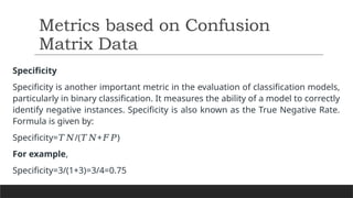
Specificity
Specificity is anotherimportant metric in the evaluation of classification models,
particularly in binary classification. It measures the ability of a model to correctly
identify negative instances. Specificity is also known as the True Negative Rate.
Formula is given by:
Specificity= /( + )
𝑇𝑁 𝑇𝑁 𝐹𝑃
For example,
Specificity=3/(1+3)
=3/4=0.75
Metrics based on Confusion
Matrix Data
19.
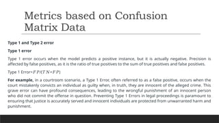
Type 1 andType 2 error
Type 1 error
Type 1 error occurs when the model predicts a positive instance, but it is actually negative. Precision is
affected by false positives, as it is the ratio of true positives to the sum of true positives and false positives.
Type 1 Error= /( + )
𝐹𝑃 𝑇𝑁 𝐹𝑃
For example, in a courtroom scenario, a Type 1 Error, often referred to as a false positive, occurs when the
court mistakenly convicts an individual as guilty when, in truth, they are innocent of the alleged crime. This
grave error can have profound consequences, leading to the wrongful punishment of an innocent person
who did not commit the offense in question. Preventing Type 1 Errors in legal proceedings is paramount to
ensuring that justice is accurately served and innocent individuals are protected from unwarranted harm and
punishment.
Metrics based on Confusion
Matrix Data
20.
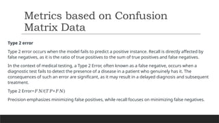
Type 2 error
Type2 error occurs when the model fails to predict a positive instance. Recall is directly affected by
false negatives, as it is the ratio of true positives to the sum of true positives and false negatives.
In the context of medical testing, a Type 2 Error, often known as a false negative, occurs when a
diagnostic test fails to detect the presence of a disease in a patient who genuinely has it. The
consequences of such an error are significant, as it may result in a delayed diagnosis and subsequent
treatment.
Type 2 Error= /( + )
𝐹𝑁 𝑇𝑃 𝐹𝑁
Precision emphasizes minimizing false positives, while recall focuses on minimizing false negatives.
Metrics based on Confusion
Matrix Data
21.
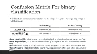
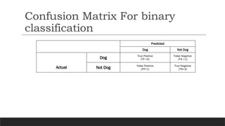
Predicted Dog PredictedNot Dog
Actual Dog True Positive (TP) False Negative (FN)
Actual Not Dog False Positive (FP) True Negative (TN)
Confusion Matrix For binary
classification
A 2X2 Confusion matrix is shown below for the image recognition having a Dog image or
Not Dog image.
•True Positive (TP): It is the total counts having both predicted and actual values are Dog.
•True Negative (TN): It is the total counts having both predicted and actual values are Not
Dog.
•False Positive (FP): It is the total counts having prediction is Dog while actually Not Dog.
•False Negative (FN): It is the total counts having prediction is Not Dog while actually, it is
Dog.
22.
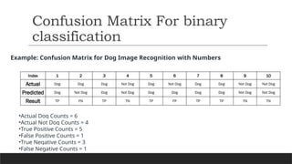
Example: Confusion Matrixfor Dog Image Recognition with Numbers
Confusion Matrix For binary
classification
Index 1 2 3 4 5 6 7 8 9 10
Actual Dog Dog Dog Not Dog Dog Not Dog Dog Dog Not Dog Not Dog
Predicted Dog Not Dog Dog Not Dog Dog Dog Dog Dog Not Dog Not Dog
Result TP FN TP TN TP FP TP TP TN TN
•Actual Dog Counts = 6
•Actual Not Dog Counts = 4
•True Positive Counts = 5
•False Positive Counts = 1
•True Negative Counts = 3
•False Negative Counts = 1
23.
Confusion Matrix Forbinary
classification
Predicted
Dog Not Dog
Actual
Dog True Positive
(TP =5)
False Negative
(FN =1)
Not Dog False Positive
(FP=1)
True Negative
(TN=3)
24.
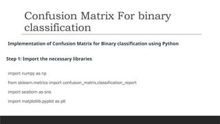
Implementation of ConfusionMatrix for Binary classification using Python
Step 1: Import the necessary libraries
import numpy as np
from sklearn.metrics import confusion_matrix,classification_report
import seaborn as sns
import matplotlib.pyplot as plt
Confusion Matrix For binary
classification
25.
Step 2: Createthe NumPy array for actual and predicted labels
actual = np.array(
['Dog','Dog','Dog','Not Dog','Dog','Not Dog','Dog','Dog','Not Dog','Not Dog'])
predicted = np.array(
['Dog','Not Dog','Dog','Not Dog','Dog','Dog','Dog','Dog','Not Dog','Not Dog'])
Confusion Matrix For binary
classification
26.
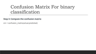
Step 3: Computethe confusion matrix
cm = confusion_matrix(actual,predicted)
Confusion Matrix For binary
classification
Confusion Matrix Forbinary
classification
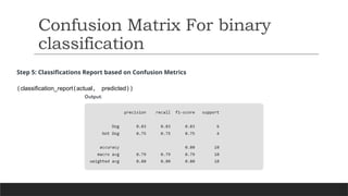
Step 5: Classifications Report based on Confusion Metrics
(classification_report(actual, predicted))
30.
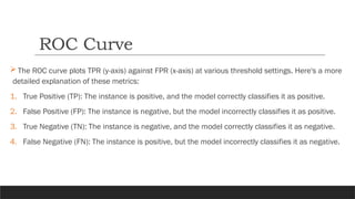
A ROC(which stands for “receiver operating characteristic”) curve is a graph that shows a
classification model performance at all classification thresholds.
It is a probability curve that plots two parameters, the True Positive Rate (TPR) against the
False Positive Rate (FPR), at different threshold values and separates a so-called ‘signal’ from
the ‘noise.’
The ROC curve plots the True Positive Rate against the False Positive Rate at different
classification thresholds.
If the user lowers the classification threshold, more items get classified as positive, which
increases both the False Positives and True Positives.
ROC Curve
31.
An ROC(Receiver Operating Characteristic) curve is a graphical representation used to evaluate the
performance of a binary classifier. It plots two key metrics:
1. True Positive Rate (TPR): Also known as sensitivity or recall, it measures the proportion of actual positives
correctly identified by the model.
It is calculated as:
TPR=True Positives/(TP)True Positives (TP) + False Negatives
2. False Positive Rate (FPR): This measures the proportion of actual negatives incorrectly identified as positives
by the model.
It is calculated as:
FPR=False Positives (FP)/False Positives (FP) + True Negatives (TN)
ROC Curve
32.
The ROCcurve plots TPR (y-axis) against FPR (x-axis) at various threshold settings. Here's a more
detailed explanation of these metrics:
1. True Positive (TP): The instance is positive, and the model correctly classifies it as positive.
2. False Positive (FP): The instance is negative, but the model incorrectly classifies it as positive.
3. True Negative (TN): The instance is negative, and the model correctly classifies it as negative.
4. False Negative (FN): The instance is positive, but the model incorrectly classifies it as negative.
ROC Curve
33.
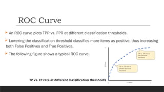
An ROCcurve plots TPR vs. FPR at different classification thresholds.
Lowering the classification threshold classifies more items as positive, thus increasing
both False Positives and True Positives.
The following figure shows a typical ROC curve.
ROC Curve
TP vs. FP rate at different classification thresholds.
34.
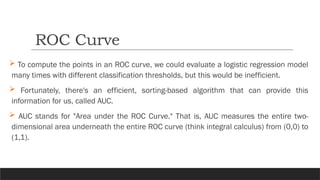
To computethe points in an ROC curve, we could evaluate a logistic regression model
many times with different classification thresholds, but this would be inefficient.
Fortunately, there's an efficient, sorting-based algorithm that can provide this
information for us, called AUC.
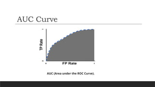
AUC stands for "Area under the ROC Curve." That is, AUC measures the entire two-
dimensional area underneath the entire ROC curve (think integral calculus) from (0,0) to
(1,1).
ROC Curve
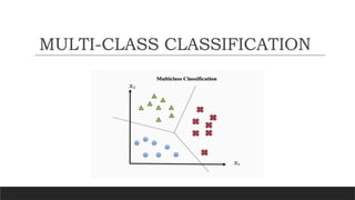
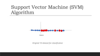
The primaryclassification technique, samples are classified into two classes.
Multiclass classification problem is the method for classifying instances into more than two
classes and each sample has to labelled as one class.
For example consider a fruit classification problems where fruit can be classified as an orange,
an apple or a banana.
Each image represents a single sample and is labelled with one of the three classes available.
Here each sample should be assigned to only one class, for example one sample can not be
both apple and banana.
MULTI-CLASS CLASSIFICATION
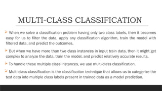
When wesolve a classification problem having only two class labels, then it becomes
easy for us to filter the data, apply any classification algorithm, train the model with
filtered data, and predict the outcomes.
But when we have more than two class instances in input train data, then it might get
complex to analyze the data, train the model, and predict relatively accurate results.
To handle these multiple class instances, we use multi-class classification.
Multi-class classification is the classification technique that allows us to categorize the
test data into multiple class labels present in trained data as a model prediction.
MULTI-CLASS CLASSIFICATION
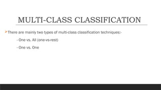
39.
There are mainlytwo types of multi-class classification techniques:-
- One vs. All (one-vs-rest)
- One vs. One
MULTI-CLASS CLASSIFICATION
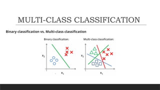
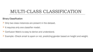
Binary Classification
Onlytwo class instances are present in the dataset.
It requires only one classifier model.
Confusion Matrix is easy to derive and understand.
Example:- Check email is spam or not, predicting gender based on height and weight.
MULTI-CLASS CLASSIFICATION
42.
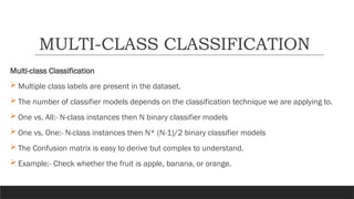
Multi-class Classification
Multipleclass labels are present in the dataset.
The number of classifier models depends on the classification technique we are applying to.
One vs. All:- N-class instances then N binary classifier models
One vs. One:- N-class instances then N* (N-1)/2 binary classifier models
The Confusion matrix is easy to derive but complex to understand.
Example:- Check whether the fruit is apple, banana, or orange.
MULTI-CLASS CLASSIFICATION
43.
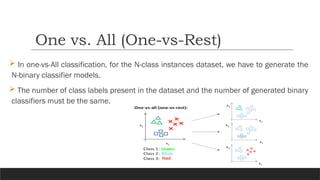
In one-vs-Allclassification, for the N-class instances dataset, we have to generate the
N-binary classifier models.
The number of class labels present in the dataset and the number of generated binary
classifiers must be the same.
One vs. All (One-vs-Rest)
44.
As shown inthe above image, consider three classes, for example, type 1 for Green,
type 2 for Blue, and type 3 for Red.
Now, generate the same number of classifiers as the class labels are present in the
dataset, So create three classifiers here for three respective classes.
• Classifier 1:- [Green] vs [Red, Blue]
• Classifier 2:- [Blue] vs [Green, Red]
• Classifier 3:- [Red] vs [Blue, Green]
One vs. All (One-vs-Rest)
45.
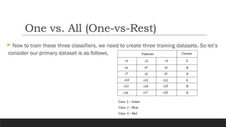
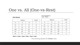
Now totrain these three classifiers, we need to create three training datasets. So let’s
consider our primary dataset is as follows,
One vs. All (One-vs-Rest)
46.
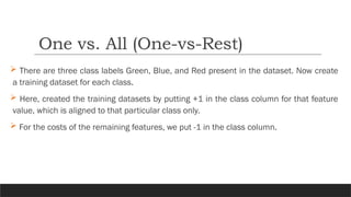
There arethree class labels Green, Blue, and Red present in the dataset. Now create
a training dataset for each class.
Here, created the training datasets by putting +1 in the class column for that feature
value, which is aligned to that particular class only.
For the costs of the remaining features, we put -1 in the class column.
One vs. All (One-vs-Rest)
47.
One vs. All(One-vs-Rest)
The training dataset for Green class
48.
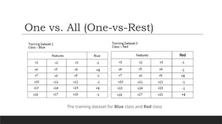
One vs. All(One-vs-Rest)
The training dataset for Blue class and Red class
49.
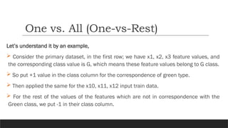
Let’s understand itby an example,
Consider the primary dataset, in the first row; we have x1, x2, x3 feature values, and
the corresponding class value is G, which means these feature values belong to G class.
So put +1 value in the class column for the correspondence of green type.
Then applied the same for the x10, x11, x12 input train data.
For the rest of the values of the features which are not in correspondence with the
Green class, we put -1 in their class column.
One vs. All (One-vs-Rest)
50.
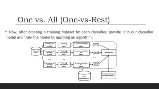
Now, aftercreating a training dataset for each classifier, provide it to our classifier
model and train the model by applying an algorithm.
One vs. All (One-vs-Rest)
51.
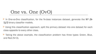
In One-vs-Oneclassification, for the N-class instances dataset, generate the N* (N-
1)/2 binary classifier models.
Using this classification approach, split the primary dataset into one dataset for each
class opposite to every other class.
Taking the above example, the classification problem has three types: Green, Blue,
and Red (N=3).
One vs. One (OvO)
52.
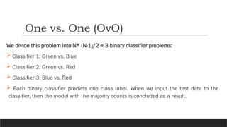
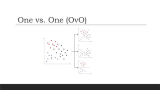
We divide thisproblem into N* (N-1)/2 = 3 binary classifier problems:
Classifier 1: Green vs. Blue
Classifier 2: Green vs. Red
Classifier 3: Blue vs. Red
Each binary classifier predicts one class label. When we input the test data to the
classifier, then the model with the majority counts is concluded as a result.
One vs. One (OvO)
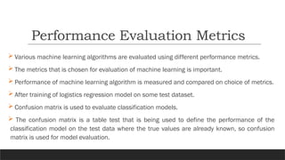
Various machinelearning algorithms are evaluated using different performance metrics.
The metrics that is chosen for evaluation of machine learning is important.
Performance of machine learning algorithm is measured and compared on choice of metrics.
After training of logistics regression model on some test dataset.
Confusion matrix is used to evaluate classification models.
The confusion matrix is a table test that is being used to define the performance of the
classification model on the test data where the true values are already known, so confusion
matrix is used for model evaluation.
Performance Evaluation Metrics
Support VectorMachine (SVM) is a powerful machine learning algorithm used for linear or
nonlinear classification, regression, and even outlier detection tasks.
SVMs can be used for a variety of tasks, such as text classification, image classification,
spam detection, handwriting identification, gene expression analysis, face detection, and
anomaly detection.
SVMs are adaptable and efficient in a variety of applications because they can manage high-
dimensional data and nonlinear relationships.
SVM algorithms are very effective in finding the maximum separating hyperplane between
the different classes available in the target feature.
Support Vector Machine (SVM)
Algorithm
57.
Support VectorMachine (SVM) is a supervised machine learning algorithm used for
both classification and regression.
Though we say regression problems as well it’s best suited for classification.
The main objective of the SVM algorithm is to find the optimal hyperplane in an N-
dimensional space that can separate the data points in different classes in the feature
space.
Support Vector Machine (SVM)
Algorithm
58.
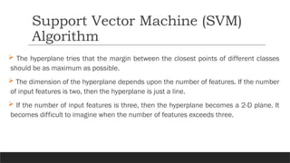
The hyperplanetries that the margin between the closest points of different classes
should be as maximum as possible.
The dimension of the hyperplane depends upon the number of features. If the number
of input features is two, then the hyperplane is just a line.
If the number of input features is three, then the hyperplane becomes a 2-D plane. It
becomes difficult to imagine when the number of features exceeds three.
Support Vector Machine (SVM)
Algorithm
59.
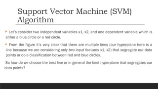
Let’s considertwo independent variables x1, x2, and one dependent variable which is
either a blue circle or a red circle.
From the figure it’s very clear that there are multiple lines (our hyperplane here is a
line because we are considering only two input features x1, x2) that segregate our data
points or do a classification between red and blue circles.
So how do we choose the best line or in general the best hyperplane that segregates our
data points?
Support Vector Machine (SVM)
Algorithm
60.
Support Vector Machine(SVM)
Algorithm
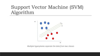
Multiple hyperplanes separate the data from two classes
61.
So wechoose the hyperplane whose distance from it to the nearest data point on each side is
maximized.
If such a hyperplane exists it is known as the maximum-margin hyperplane/hard margin.
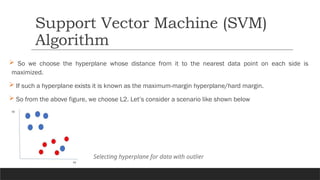
So from the above figure, we choose L2. Let’s consider a scenario like shown below
Support Vector Machine (SVM)
Algorithm
Selecting hyperplane for data with outlier
62.
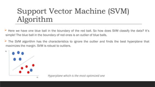
Here wehave one blue ball in the boundary of the red ball. So how does SVM classify the data? It’s
simple! The blue ball in the boundary of red ones is an outlier of blue balls.
The SVM algorithm has the characteristics to ignore the outlier and finds the best hyperplane that
maximizes the margin. SVM is robust to outliers.
Support Vector Machine (SVM)
Algorithm
Hyperplane which is the most optimized one
63.
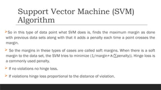
So in thistype of data point what SVM does is, finds the maximum margin as done
with previous data sets along with that it adds a penalty each time a point crosses the
margin.
So the margins in these types of cases are called soft margins. When there is a soft
margin to the data set, the SVM tries to minimize (1/margin+ (∑penalty)). Hinge loss is
∧
a commonly used penalty.
If no violations no hinge loss.
If violations hinge loss proportional to the distance of violation.
Support Vector Machine (SVM)
Algorithm
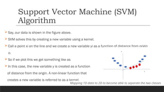
Say, our datais shown in the figure above.
SVM solves this by creating a new variable using a kernel.
Call a point xi on the line and we create a new variable yi as a function of distance from origin
o.
So if we plot this we get something like as
In this case, the new variable y is created as a function
of distance from the origin. A non-linear function that
creates a new variable is referred to as a kernel.
Support Vector Machine (SVM)
Algorithm
Mapping 1D data to 2D to become able to separate the two classes
66.
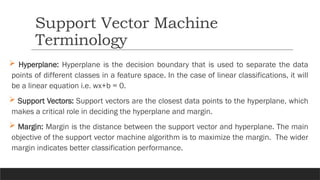
Hyperplane: Hyperplaneis the decision boundary that is used to separate the data
points of different classes in a feature space. In the case of linear classifications, it will
be a linear equation i.e. wx+b = 0.
Support Vectors: Support vectors are the closest data points to the hyperplane, which
makes a critical role in deciding the hyperplane and margin.
Margin: Margin is the distance between the support vector and hyperplane. The main
objective of the support vector machine algorithm is to maximize the margin. The wider
margin indicates better classification performance.
Support Vector Machine
Terminology
67.
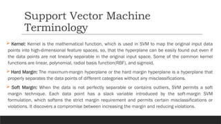
Kernel: Kernelis the mathematical function, which is used in SVM to map the original input data
points into high-dimensional feature spaces, so, that the hyperplane can be easily found out even if
the data points are not linearly separable in the original input space. Some of the common kernel
functions are linear, polynomial, radial basis function(RBF), and sigmoid.
Hard Margin: The maximum-margin hyperplane or the hard margin hyperplane is a hyperplane that
properly separates the data points of different categories without any misclassifications.
Soft Margin: When the data is not perfectly separable or contains outliers, SVM permits a soft
margin technique. Each data point has a slack variable introduced by the soft-margin SVM
formulation, which softens the strict margin requirement and permits certain misclassifications or
violations. It discovers a compromise between increasing the margin and reducing violations.
Support Vector Machine
Terminology
68.
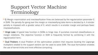
C: Marginmaximization and misclassification fines are balanced by the regularization parameter C
in SVM. The penalty for going over the margin or misclassifying data items is decided by it. A stricter
penalty is imposed with a greater value of C, which results in a smaller margin and perhaps fewer
misclassifications.
Hinge Loss: A typical loss function in SVMs is hinge loss. It punishes incorrect classifications or
margin violations. The objective function in SVM is frequently formed by combining it with the
regularization term.
Dual Problem: A dual Problem of the optimization problem that requires locating the Lagrange
multipliers related to the support vectors can be used to solve SVM. The dual formulation enables
the use of kernel tricks and more effective computing.
Support Vector Machine
Terminology
69.
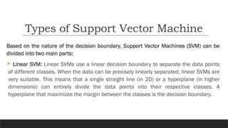
Based on thenature of the decision boundary, Support Vector Machines (SVM) can be
divided into two main parts:
Linear SVM: Linear SVMs use a linear decision boundary to separate the data points
of different classes. When the data can be precisely linearly separated, linear SVMs are
very suitable. This means that a single straight line (in 2D) or a hyperplane (in higher
dimensions) can entirely divide the data points into their respective classes. A
hyperplane that maximizes the margin between the classes is the decision boundary.
Types of Support Vector Machine
70.
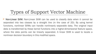
Non-Linear SVM:Non-Linear SVM can be used to classify data when it cannot be
separated into two classes by a straight line (in the case of 2D). By using kernel
functions, nonlinear SVMs can handle nonlinearly separable data. The original input
data is transformed by these kernel functions into a higher-dimensional feature space,
where the data points can be linearly separated. A linear SVM is used to locate a
nonlinear decision boundary in this modified space.
Types of Support Vector Machine
71.
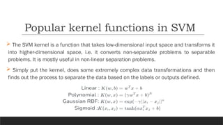
The SVMkernel is a function that takes low-dimensional input space and transforms it
into higher-dimensional space, i.e. it converts non-separable problems to separable
problems. It is mostly useful in non-linear separation problems.
Simply put the kernel, does some extremely complex data transformations and then
finds out the process to separate the data based on the labels or outputs defined.
Popular kernel functions in SVM
72.
Effective inhigh-dimensional cases.
Its memory is efficient as it uses a subset of training points in the decision function
called support vectors.
Different kernel functions can be specified for the decision functions and it’s possible
to specify custom kernels.
Advantages of SVM
73.
Logistic regressionis a supervised machine learning algorithm used for classification
tasks where the goal is to predict the probability that an instance belongs to a given
class or not.
Logistic regression is a statistical algorithm which analyzes the relationship between
two data factors.
Logistic regression is used for binary classification and uses the sigmoid function,
which takes input as independent variables and produces a probability value between 0
and 1.
Logistic Regression
74.
Logistic regression isused for binary classification where we use sigmoid function, that
takes input as independent variables and produces a probability value between 0 and
1.
For example, we have two classes Class 0 and Class 1 if the value of the logistic
function for an input is greater than 0.5 (threshold value) then it belongs to Class 1
otherwise it belongs to Class 0.
It’s referred to as regression because it is the extension of linear regression but is
mainly used for classification problems.
Logistic Regression
75.
Logistic regressionpredicts the output of a categorical dependent variable.
Therefore, the outcome must be a categorical or discrete value.
It can be either Yes or No, 0 or 1, true or False, etc. but instead of giving the exact
value as 0 and 1, it gives the probabilistic values which lie between 0 and 1.
In Logistic regression, instead of fitting a regression line, fit an “S” shaped logistic
function, which predicts two maximum values (0 or 1).
Key Points:
76.
The sigmoidfunction is a mathematical function used to map the predicted values to
probabilities.
It maps any real value into another value within a range of 0 and 1.
The value of the logistic regression must be between 0 and 1, which cannot go beyond this limit,
so it forms a curve like the “S” form.
The S-form curve is called the Sigmoid function or the logistic function.
In logistic regression, use the concept of the threshold value, which defines the probability of
either 0 or 1. Such as values above the threshold value tends to 1, and a value below the threshold
values tends to 0.
Logistic Function – Sigmoid
Function
77.
based on thecategories, Logistic Regression can be classified into three types:
1. Binomial: In binomial Logistic regression, there can be only two possible
types of dependent variables, such as 0 or 1, Pass or Fail, etc.
2. Multinomial: In multinomial Logistic regression, there can be 3 or more
possible unordered types of the dependent variable, such as “cat”, “dogs”, or
“sheep”
3. Ordinal: In ordinal Logistic regression, there can be 3 or more possible
ordered types of dependent variables, such as “low”, “Medium”, or “High”.
Types of Logistic Regression
78.
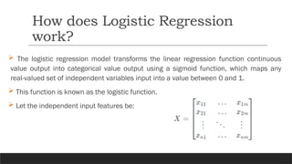
The logisticregression model transforms the linear regression function continuous
value output into categorical value output using a sigmoid function, which maps any
real-valued set of independent variables input into a value between 0 and 1.
This function is known as the logistic function.
Let the independent input features be:
How does Logistic Regression
work?
79.
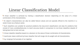
and the dependentvariable is Y having only binary value i.e. 0 or 1.
then, apply the multi-linear function to the input variables X.
Here xiis the ith
observation of X, wi
= [w1
, w2
, w3
, ,
⋯ wm
] is the weights or Coefficient, and b is
the bias term also known as intercept. simply this can be represented as the dot product of
weight and bias.
How does Logistic Regression
work?
80.
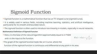
Sigmoid function isa mathematical function that has an “S”-shaped curve (sigmoid curve).
It is widely used in various fields, including machine learning, statistics, and artificial intelligence,
particularly for its smooth and bounded nature.
The sigmoid function is often used to introduce non-linearity in models, especially in neural networks.
Mathematical Definition of Sigmoid Function
Here, e is the base of the natural logarithm (approximately equal to 2.71828),
and x is the input to the function.
The graph of the sigmoid function looks like an S curve, where the
function of the sigmoid function is continuous and differential at any point in its area.
Sigmoid Function
81.
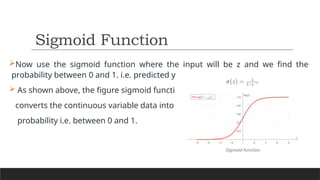
Now use thesigmoid function where the input will be z and we find the
probability between 0 and 1. i.e. predicted y.
As shown above, the figure sigmoid function
converts the continuous variable data into the
probability i.e. between 0 and 1.
Sigmoid Function
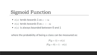
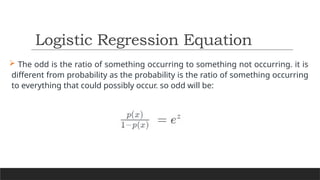
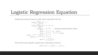
The oddis the ratio of something occurring to something not occurring. it is
different from probability as the probability is the ratio of something occurring
to everything that could possibly occur. so odd will be:
Logistic Regression Equation


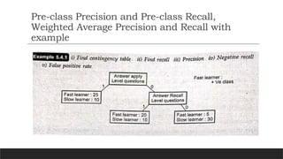
![Step 2: Create the NumPy array for actual and predicted labels
actual = np.array(
['Dog','Dog','Dog','Not Dog','Dog','Not Dog','Dog','Dog','Not Dog','Not Dog'])
predicted = np.array(
['Dog','Not Dog','Dog','Not Dog','Dog','Dog','Dog','Dog','Not Dog','Not Dog'])
Confusion Matrix For binary
classification](https://image.slidesharecdn.com/mlunit2kunal-250709102355-5d244cb7/85/machine-Learning-subject-of-third-year-information-technology-unit-2-pptx-25-320.jpg)
![plt.gca().xaxis.set_label_position('top')
plt.xlabel('Prediction', fontsize=13)
plt.gca().xaxis.tick_top()
plt.gca().figure.subplots_adjust(bottom=0.2)
plt.gca().figure.text(0.5, 0.05, 'Prediction',
ha='center', fontsize=13)
plt.show()
Confusion Matrix For binary
classification
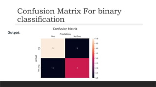
Step 4: Plot the confusion matrix with the
help of the seaborn
heatmapsns.heatmap(cm,
annot=True,
fmt='g',
xticklabels=['Dog','Not Dog'],
yticklabels=['Dog','Not Dog'])
plt.ylabel('Actual', fontsize=13)
plt.title('Confusion Matrix', fontsize=17,
pad=20)](https://image.slidesharecdn.com/mlunit2kunal-250709102355-5d244cb7/85/machine-Learning-subject-of-third-year-information-technology-unit-2-pptx-27-320.jpg)
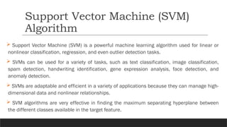
![As shown in the above image, consider three classes, for example, type 1 for Green,
type 2 for Blue, and type 3 for Red.
Now, generate the same number of classifiers as the class labels are present in the
dataset, So create three classifiers here for three respective classes.
• Classifier 1:- [Green] vs [Red, Blue]
• Classifier 2:- [Blue] vs [Green, Red]
• Classifier 3:- [Red] vs [Blue, Green]
One vs. All (One-vs-Rest)](https://image.slidesharecdn.com/mlunit2kunal-250709102355-5d244cb7/85/machine-Learning-subject-of-third-year-information-technology-unit-2-pptx-44-320.jpg)
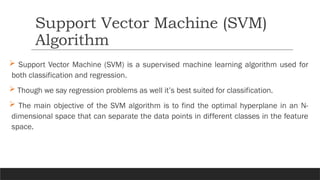
![and the dependent variable is Y having only binary value i.e. 0 or 1.
then, apply the multi-linear function to the input variables X.
Here xiis the ith
observation of X, wi
= [w1
, w2
, w3
, ,
⋯ wm
] is the weights or Coefficient, and b is
the bias term also known as intercept. simply this can be represented as the dot product of
weight and bias.
How does Logistic Regression
work?](https://image.slidesharecdn.com/mlunit2kunal-250709102355-5d244cb7/85/machine-Learning-subject-of-third-year-information-technology-unit-2-pptx-79-320.jpg)