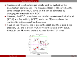
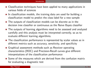
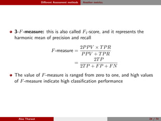
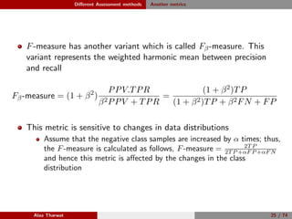
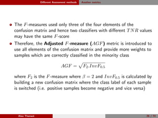
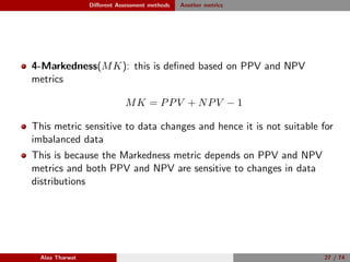
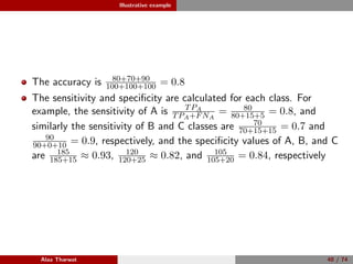
This document provides a detailed tutorial on classification assessment methods. It discusses key classification performance metrics like accuracy, sensitivity, specificity, and how they are calculated using a confusion matrix. It notes that some metrics like accuracy are sensitive to imbalanced data, while other metrics like geometric mean are more suitable. The document also introduces different assessment methods for classification like receiver operating characteristic (ROC) curves and precision-recall curves. It provides examples of how to interpret these performance evaluation techniques.

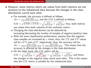


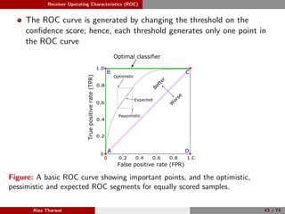
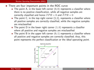
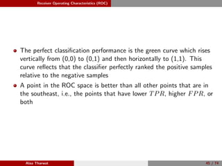
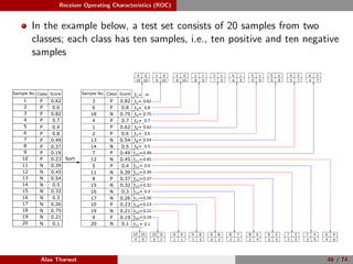
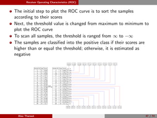
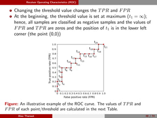
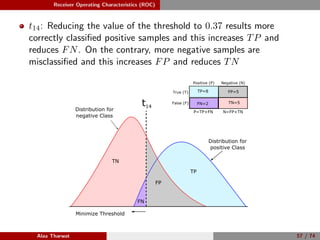
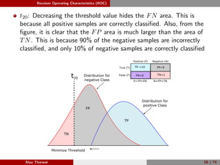
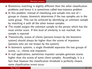
![Receiver Operating Characteristics (ROC)
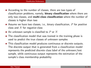
1: Given a set of test samples (Stest = {s1, s2, . . . , sN }), where N is the
total number of test samples, P and N represent the total number of
positive and negative samples, respectively.
2: Sort the samples corresponding to their scores, Ssorted is the sorted
samples.
3: FP ← 0, TP ← 0, fprev ← −∞, and ROC = [ ].
4: for i = 1 to |Ssorted| do
5: if f(i) = fprev then
6: ROC(i) ← (FP
N , TP
P ), fprev ← f(i)
7: end if
8: if Ssorted(i) is a positive sample then
9: TP ← TP + 1.
10: else
11: FP ← FP + 1.
12: end if
13: end for
14: ROC(i) ← (FP
N , TP
P ).
Alaa Tharwat 59 / 74](https://image.slidesharecdn.com/classificationassessmentmethods1-200108090615/85/Classification-assessment-methods-60-320.jpg)