fdfsdf

1. Evaluation Measures in Machine
Learning

2. In classification problems, we use two types of algorithms
(dependent on the kind of output it creates):
• Class output: Algorithms like SVM and KNN create a class
output. For instance, in a binary classification problem, the
outputs will be either 0 or 1.
• Probability output: Algorithms like Logistic Regression,
Random Forest, Gradient Boosting, Adaboost etc. give
probability outputs. Converting probability outputs to class
output is just a matter of creating a threshold probability.
In regression problems, the output is always continuous in
nature and requires no further treatment.

3. Classification metrics
• Classification models have discrete output, so
we need a metric that compares discrete
classes in some form. Classification
Metrics evaluate a model’s performance and
tell you how good or bad the classification is,
but each of them evaluates it in a different
way.

4. • Accuracy
• Confusion Matrix (not a metric but
fundamental to others)
• Precision and Recall
• F1-score
• AU-ROC

5. Accuracy
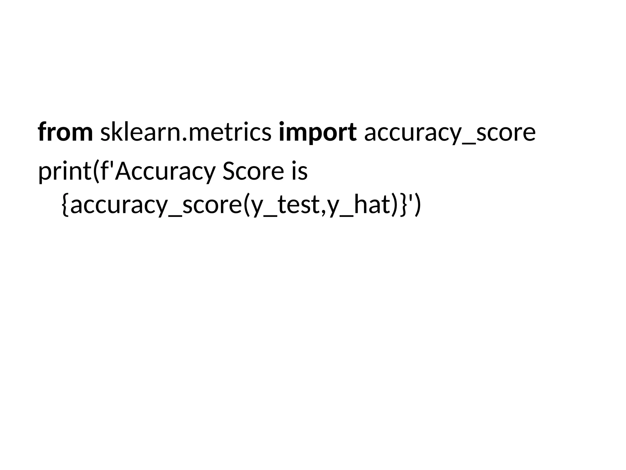
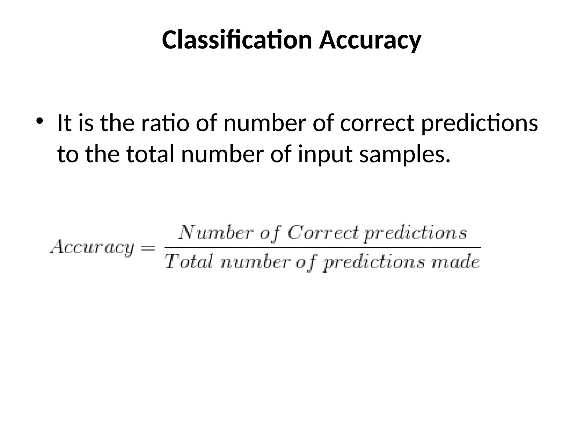
• Classification accuracy is perhaps the simplest
metric to use and implement and is defined as
the number of correct predictions divided by
the total number of predictions, multiplied by
100.
• We can implement this by comparing ground
truth and predicted values.

6. from sklearn.metrics import accuracy_score
print(f'Accuracy Score is
{accuracy_score(y_test,y_hat)}')

7. Classification Accuracy
• It is the ratio of number of correct predictions
to the total number of input samples.

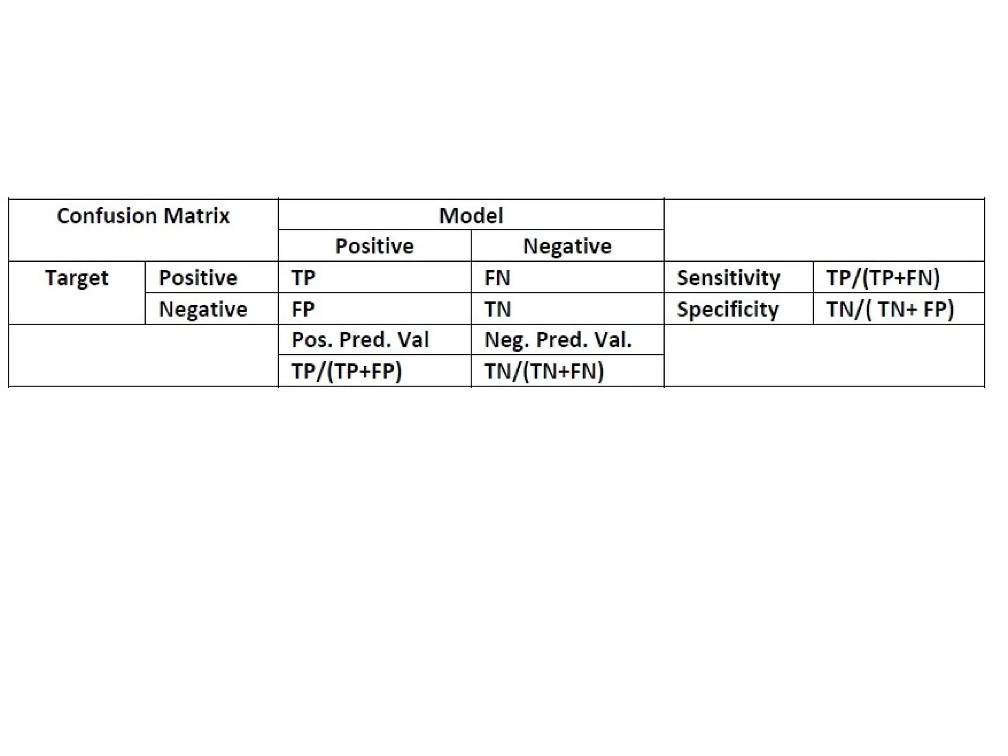
8. Confusion Matrix
• Confusion Matrix is a tabular visualization of
the ground-truth labels versus model predictions.
Each row of the confusion matrix represents the
instances in a predicted class and each column
represents the instances in an actual class. Confusion
Matrix is not exactly a performance metric but sort of
a basis on which other metrics evaluate the results.
• In order to understand the confusion matrix, we need
to set some value for the null hypothesis as an
assumption.

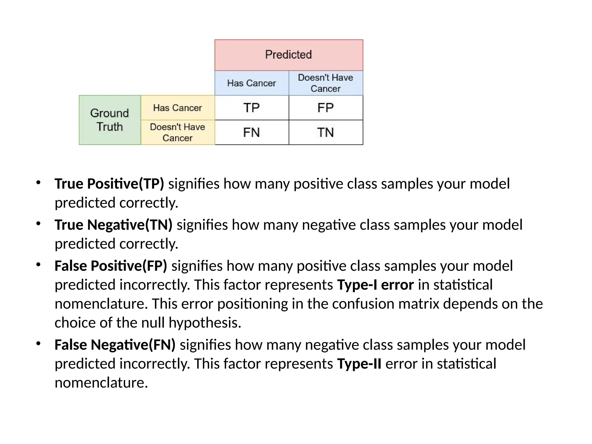
9. • True Positive(TP) signifies how many positive class samples your model
predicted correctly.
• True Negative(TN) signifies how many negative class samples your model
predicted correctly.
• False Positive(FP) signifies how many positive class samples your model
predicted incorrectly. This factor represents Type-I error in statistical
nomenclature. This error positioning in the confusion matrix depends on the
choice of the null hypothesis.
• False Negative(FN) signifies how many negative class samples your model
predicted incorrectly. This factor represents Type-II error in statistical
nomenclature.

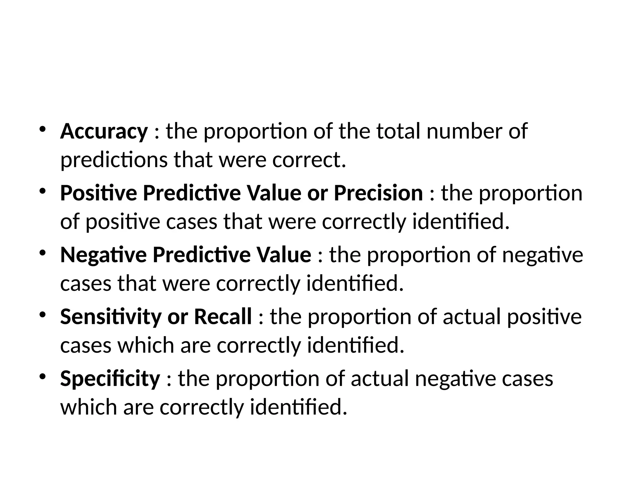
10. • Accuracy : the proportion of the total number of
predictions that were correct.
• Positive Predictive Value or Precision : the proportion
of positive cases that were correctly identified.
• Negative Predictive Value : the proportion of negative
cases that were correctly identified.
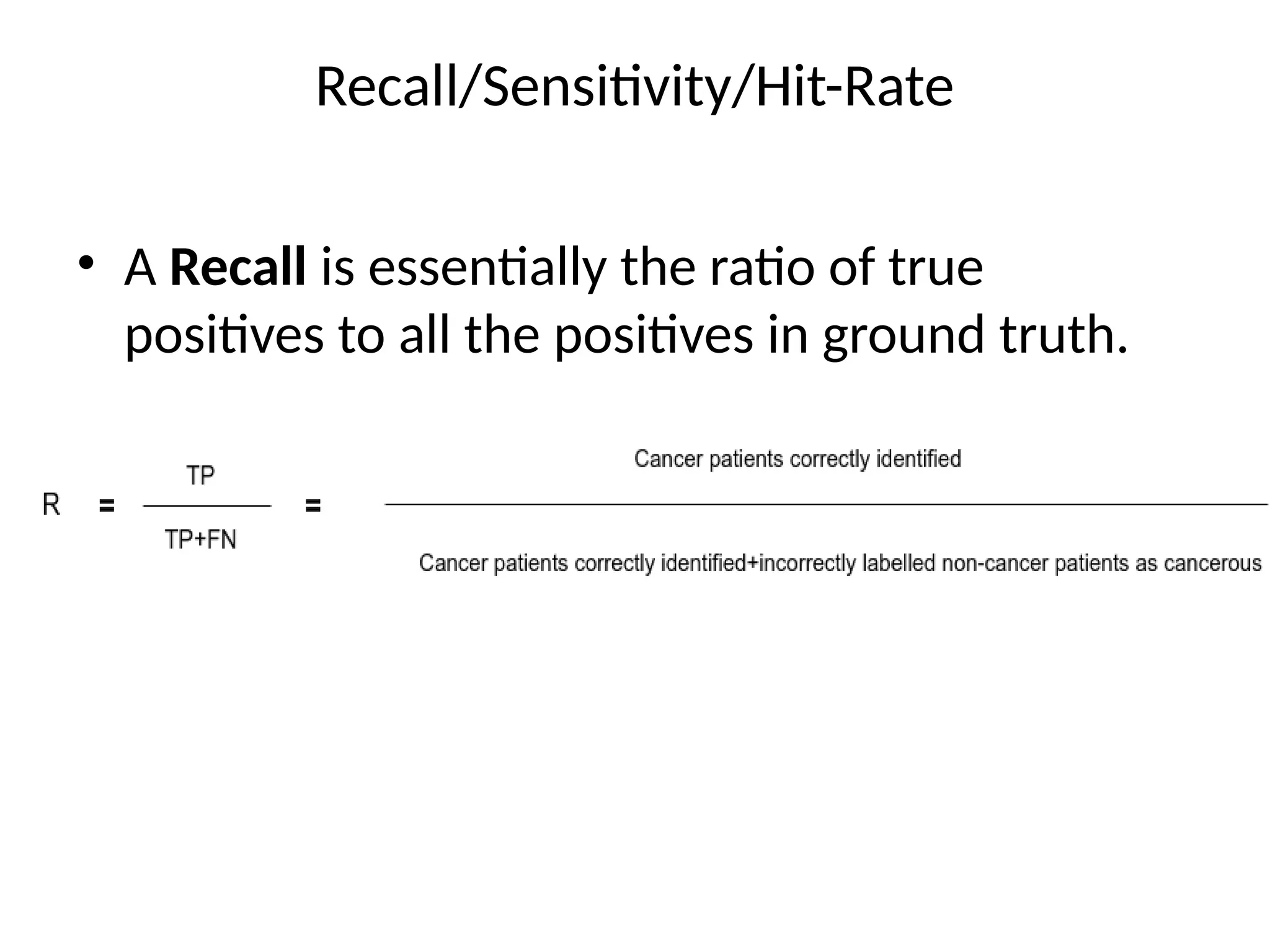
• Sensitivity or Recall : the proportion of actual positive
cases which are correctly identified.
• Specificity : the proportion of actual negative cases
which are correctly identified.

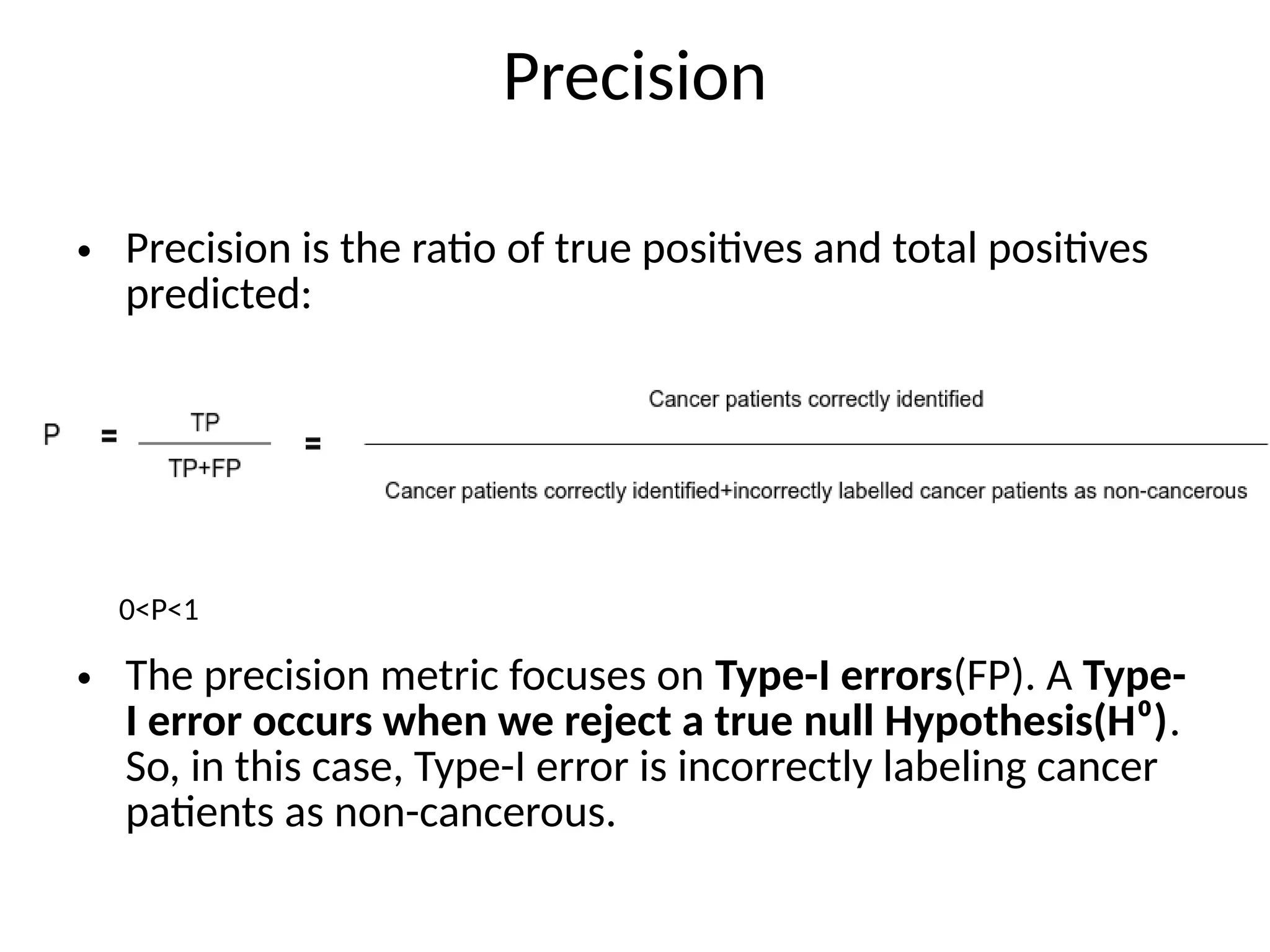
12. Precision
• Precision is the ratio of true positives and total positives
predicted:
• The precision metric focuses on Type-I errors(FP). A Type-
I error occurs when we reject a true null Hypothesis(H⁰).
So, in this case, Type-I error is incorrectly labeling cancer
patients as non-cancerous.
0<P<1

13. • A precision score towards 1 will signify that your model
didn’t miss any true positives, and is able to classify
well between correct and incorrect labeling of cancer
patients. What it cannot measure is the existence of
Type-II error, which is false negatives – cases when a
non-cancerous patient is identified as cancerous.
• A low precision score (<0.5) means your classifier has a
high number of false positives which can be an
outcome of imbalanced class or untuned model
hyperparameters.

14. Recall/Sensitivity/Hit-Rate
• A Recall is essentially the ratio of true
positives to all the positives in ground truth.

15. Example
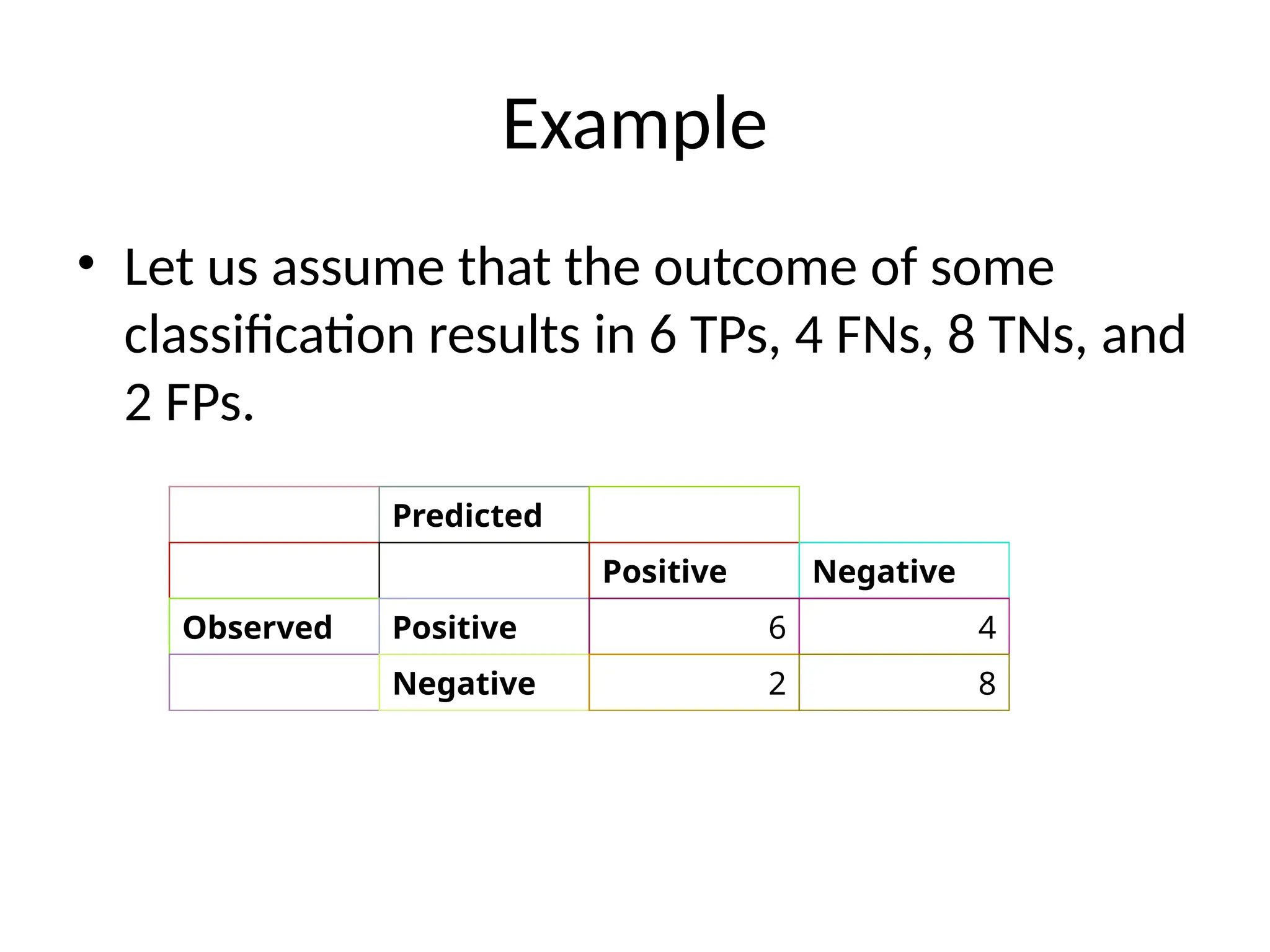
• Let us assume that the outcome of some
classification results in 6 TPs, 4 FNs, 8 TNs, and
2 FPs.
Predicted
Positive Negative
Observed Positive 6 4
Negative 2 8

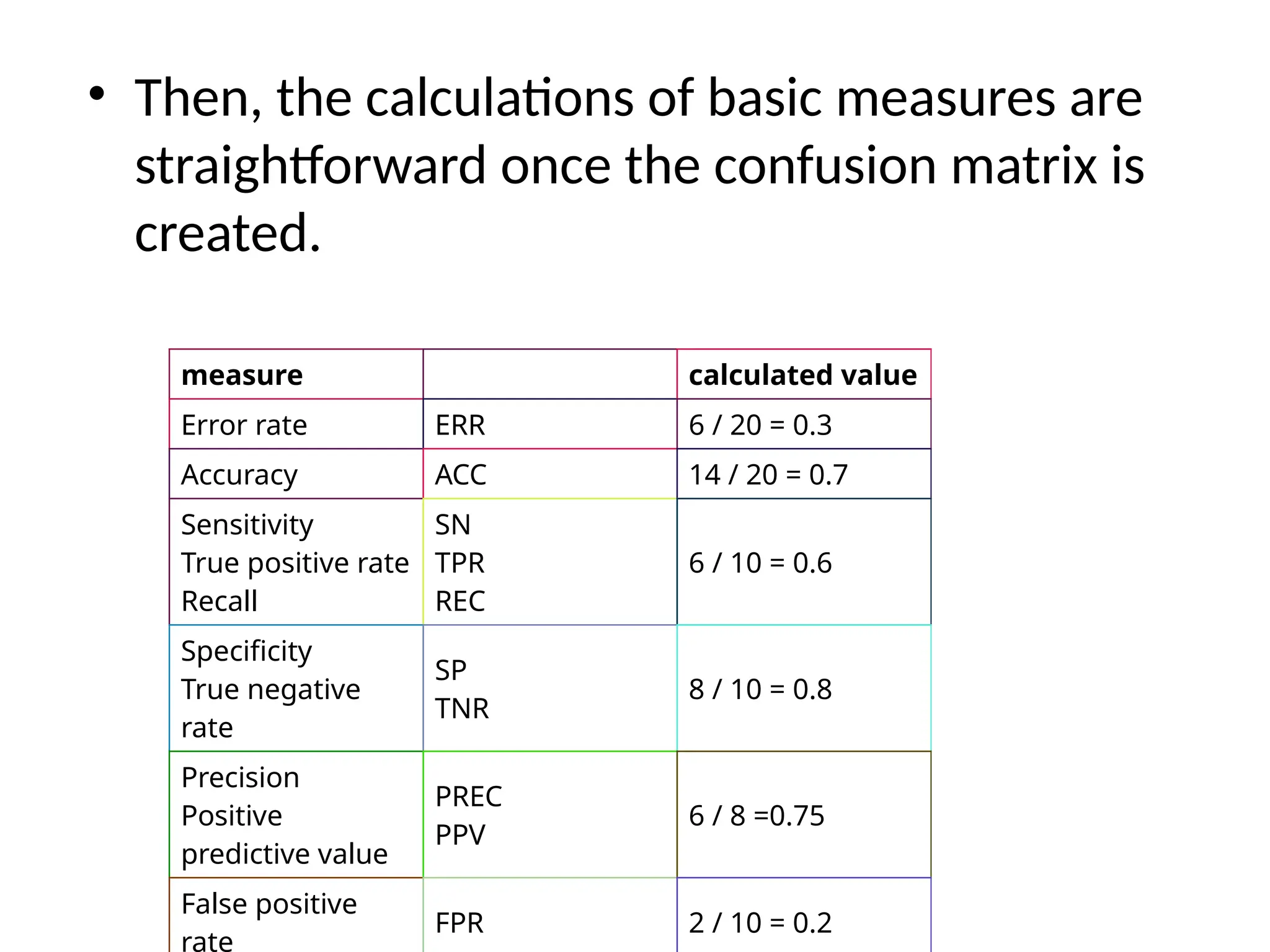
16. • Then, the calculations of basic measures are
straightforward once the confusion matrix is
created.
measure calculated value
Error rate ERR 6 / 20 = 0.3
Accuracy ACC 14 / 20 = 0.7
Sensitivity
True positive rate
Recall
SN
TPR
REC
6 / 10 = 0.6
Specificity
True negative
rate
SP
TNR
8 / 10 = 0.8
Precision
Positive
predictive value
PREC
PPV
6 / 8 =0.75
False positive
rate
FPR 2 / 10 = 0.2

17. Example
• Let’s say you are building a model that detects
whether a person has diabetes or not. After
the train-test split, you got a test set of length
100, out of which 70 data points are labeled
positive (1), and 30 data points are labelled
negative (0).

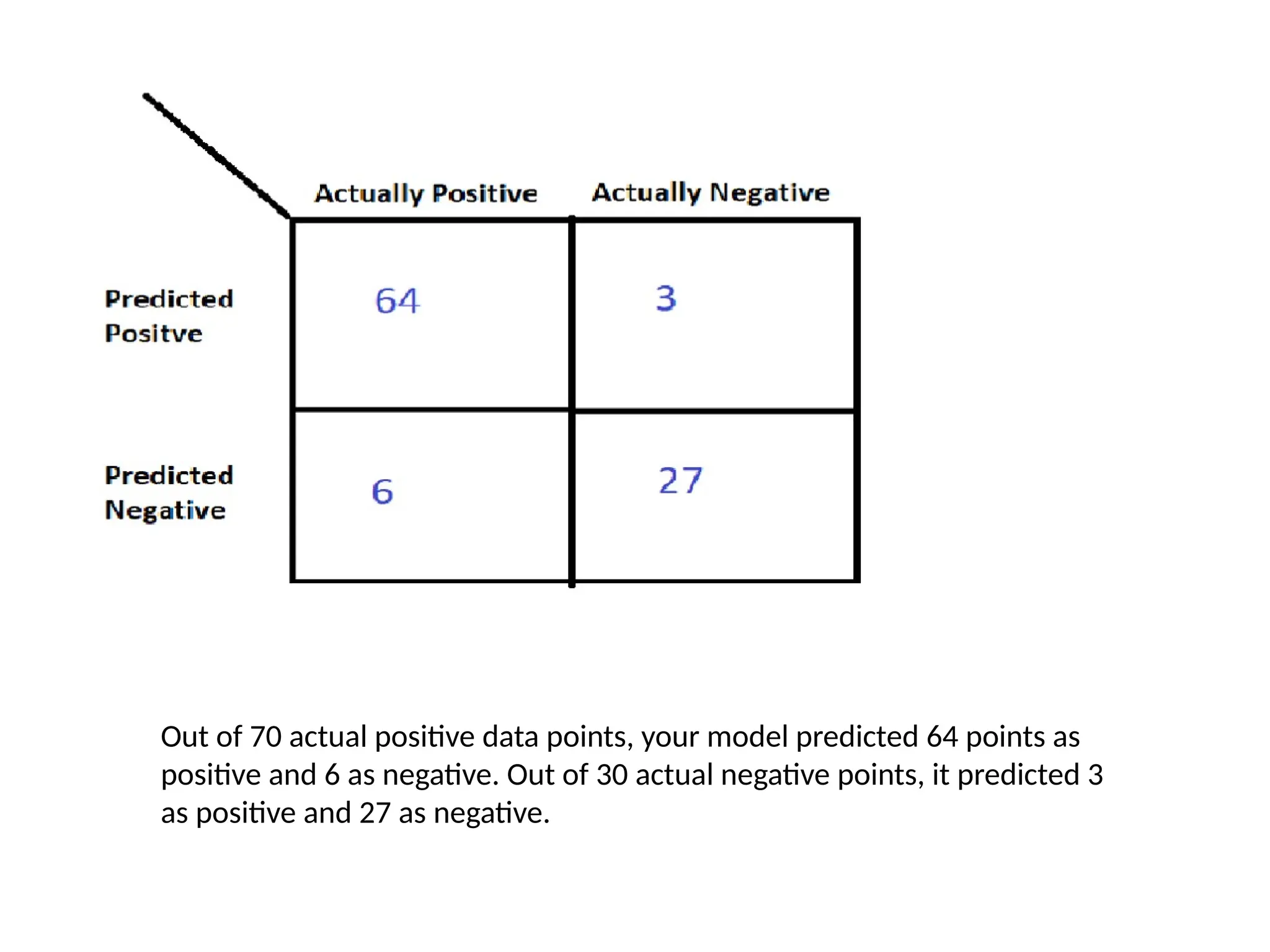
18. Out of 70 actual positive data points, your model predicted 64 points as
positive and 6 as negative. Out of 30 actual negative points, it predicted 3
as positive and 27 as negative.

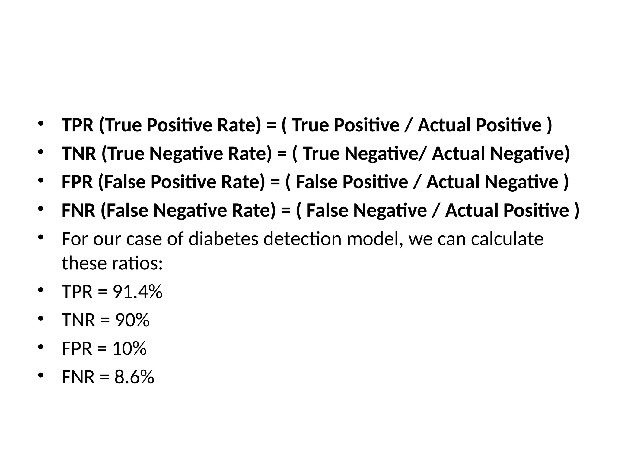
19. • TPR (True Positive Rate) = ( True Positive / Actual Positive )
• TNR (True Negative Rate) = ( True Negative/ Actual Negative)
• FPR (False Positive Rate) = ( False Positive / Actual Negative )
• FNR (False Negative Rate) = ( False Negative / Actual Positive )
• For our case of diabetes detection model, we can calculate
these ratios:
• TPR = 91.4%
• TNR = 90%
• FPR = 10%
• FNR = 8.6%

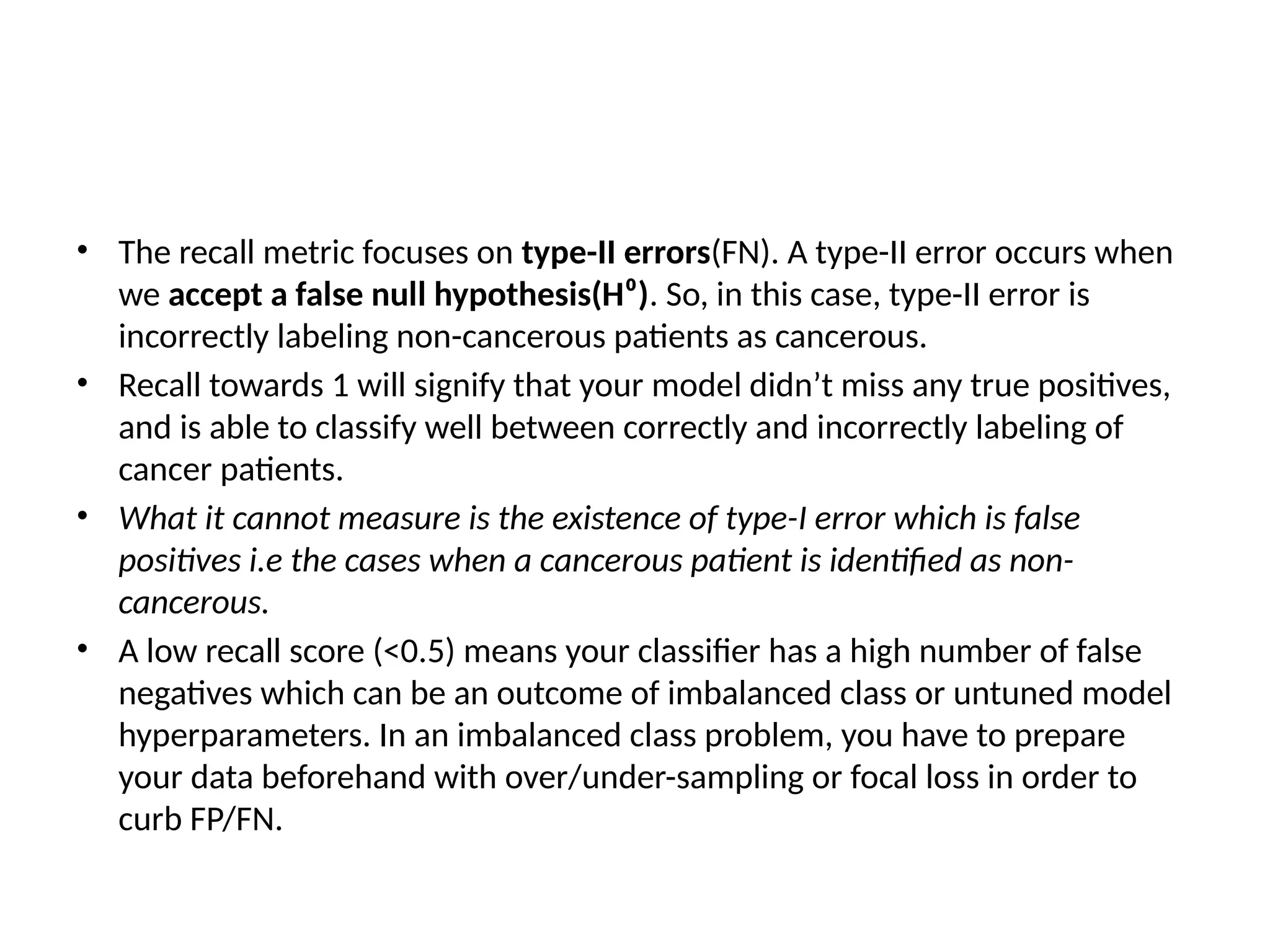
20. • The recall metric focuses on type-II errors(FN). A type-II error occurs when
we accept a false null hypothesis(H⁰). So, in this case, type-II error is
incorrectly labeling non-cancerous patients as cancerous.
• Recall towards 1 will signify that your model didn’t miss any true positives,
and is able to classify well between correctly and incorrectly labeling of
cancer patients.
• What it cannot measure is the existence of type-I error which is false
positives i.e the cases when a cancerous patient is identified as non-
cancerous.
• A low recall score (<0.5) means your classifier has a high number of false
negatives which can be an outcome of imbalanced class or untuned model
hyperparameters. In an imbalanced class problem, you have to prepare
your data beforehand with over/under-sampling or focal loss in order to
curb FP/FN.

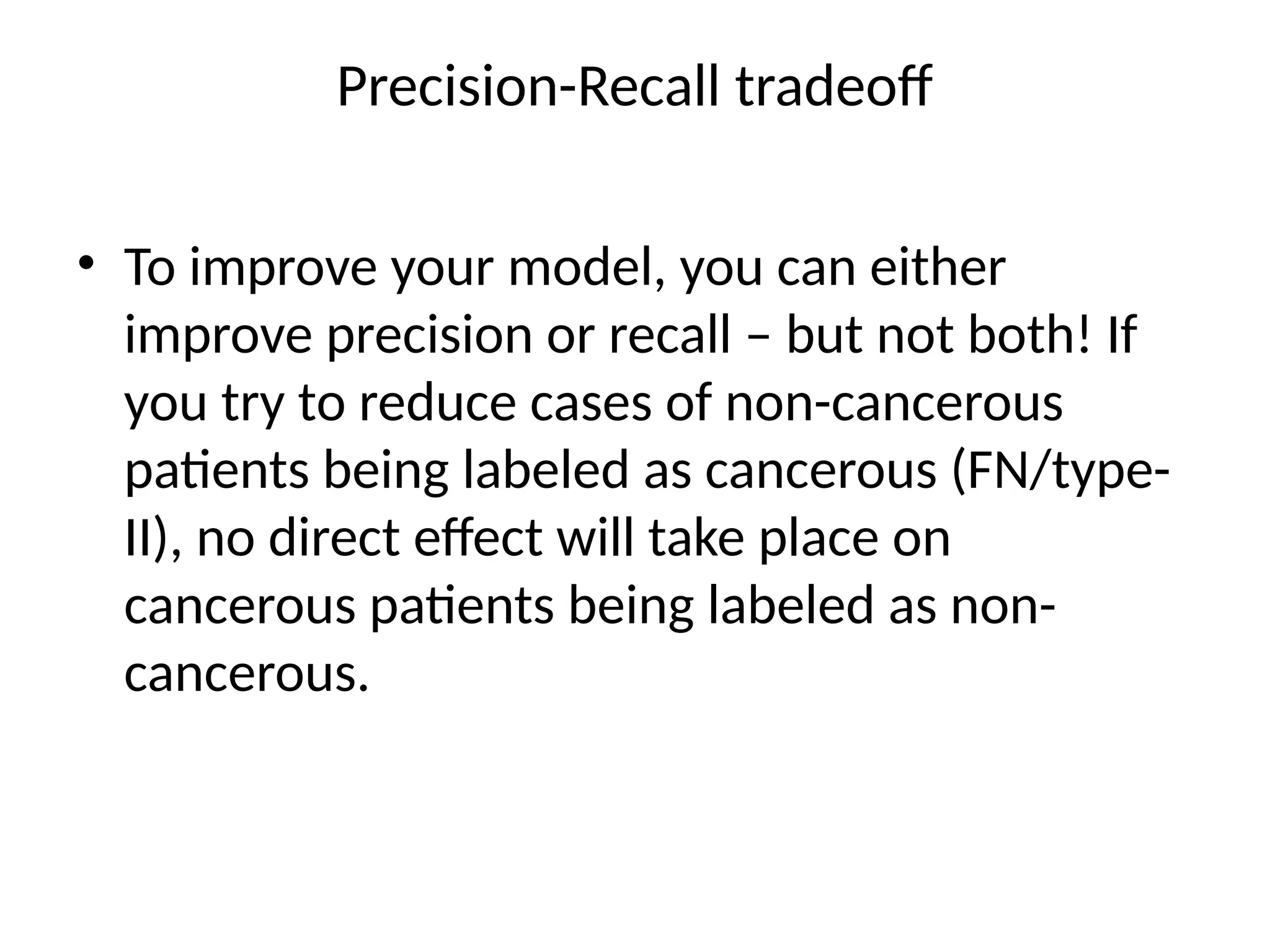
21. Precision-Recall tradeoff
• To improve your model, you can either
improve precision or recall – but not both! If
you try to reduce cases of non-cancerous
patients being labeled as cancerous (FN/type-
II), no direct effect will take place on
cancerous patients being labeled as non-
cancerous.

23. from sklearn.metrics import plot_precision_recall_curve
disp = plot_precision_recall_curve(clf, X, y)
disp.ax_.set_title('2-class Precision-Recall curve: '
'AP={0:0.2f}'.format(precision))

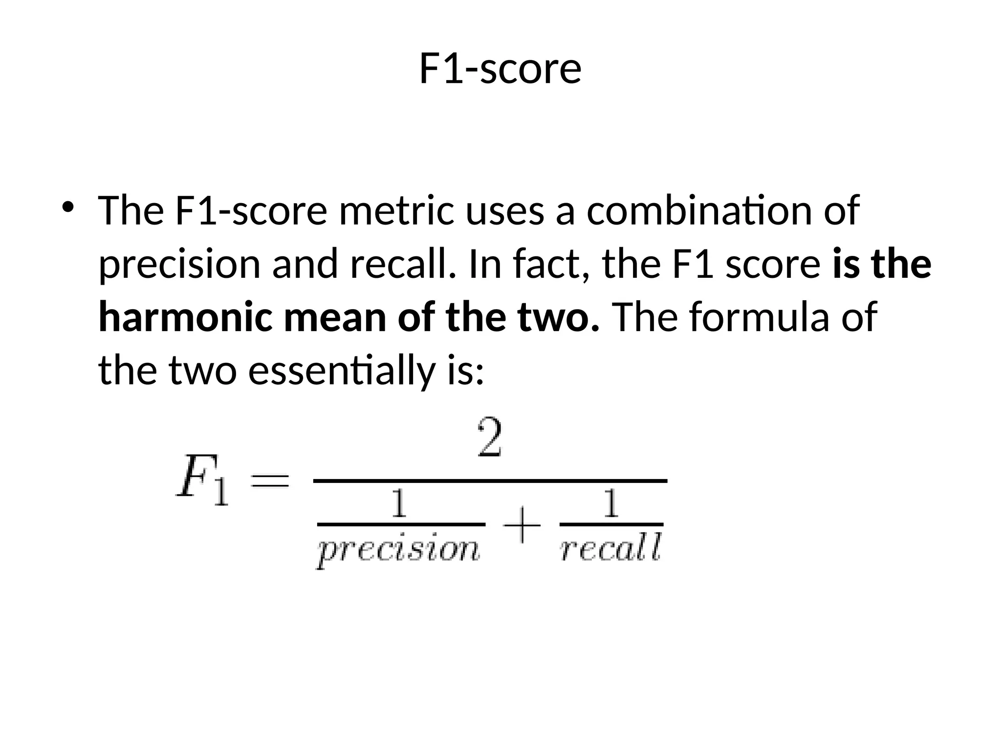
24. F1-score
• The F1-score metric uses a combination of
precision and recall. In fact, the F1 score is the
harmonic mean of the two. The formula of
the two essentially is:

25. • Now, a high F1 score symbolizes a high precision as
well as high recall. It presents a good balance
between precision and recall and gives good results
on imbalanced classification problems.
• A low F1 score tells you (almost) nothing—it only
tells you about performance at a threshold. Low
recall means we didn’t try to do well on very much
of the entire test set. Low precision means that,
among the cases we identified as positive cases, we
didn’t get many of them right.

26. • High F1 means we likely have high precision and
recall on a large portion of the decision (which is
informative). With low F1, it’s unclear what the
problem is (low precision or low recall?), and whether
the model suffers from type-I or type-II error.
• it’s widely used, and considered a fine metric to
converge onto a decision. Using FPR (false positive
rates) along with F1 will help curb type-I errors, and
you’ll get an idea about the villain behind your low F1
score.

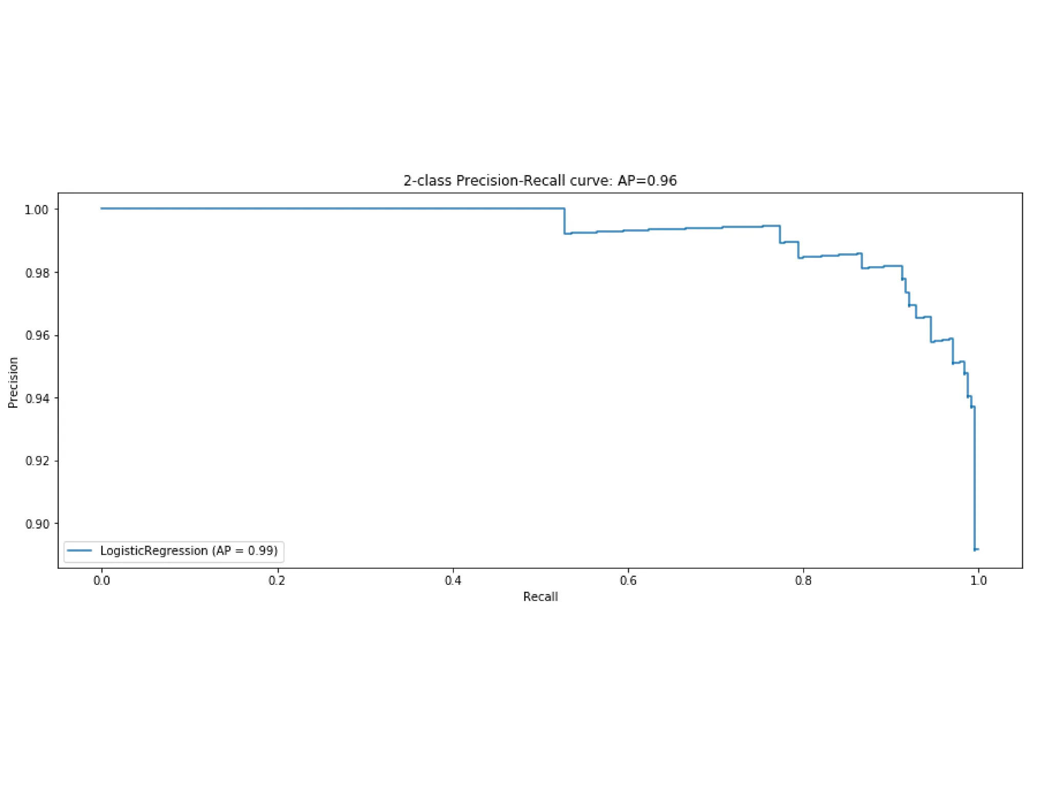
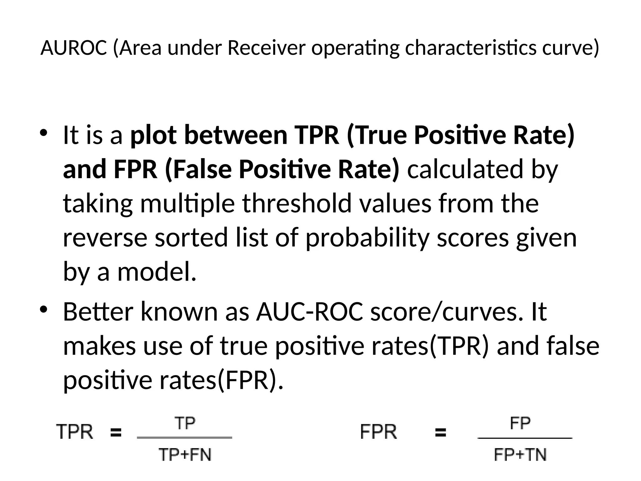
27. AUROC (Area under Receiver operating characteristics curve)
• It is a plot between TPR (True Positive Rate)
and FPR (False Positive Rate) calculated by
taking multiple threshold values from the
reverse sorted list of probability scores given
by a model.
• Better known as AUC-ROC score/curves. It
makes use of true positive rates(TPR) and false
positive rates(FPR).

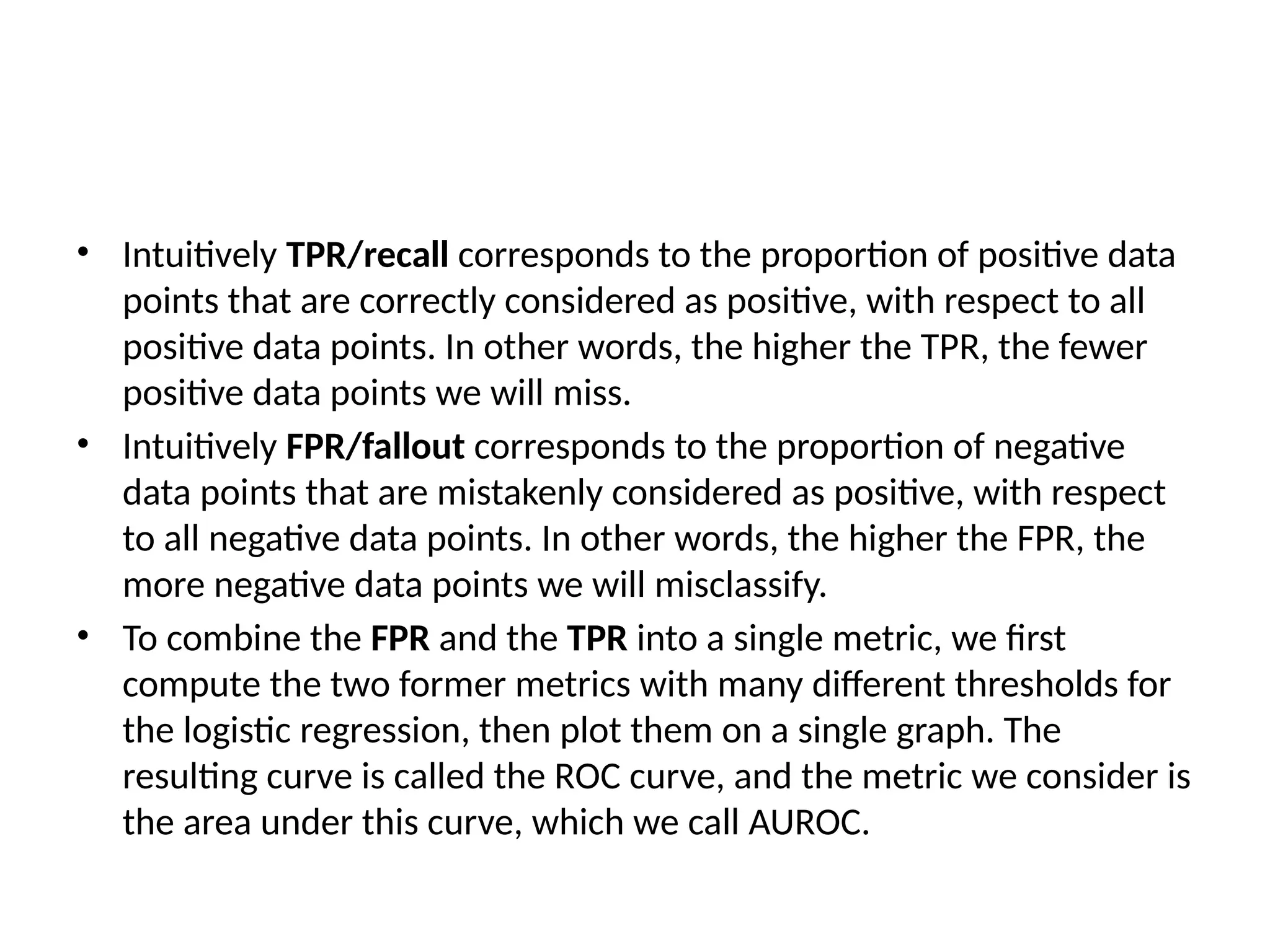
29. • Intuitively TPR/recall corresponds to the proportion of positive data
points that are correctly considered as positive, with respect to all
positive data points. In other words, the higher the TPR, the fewer
positive data points we will miss.
• Intuitively FPR/fallout corresponds to the proportion of negative
data points that are mistakenly considered as positive, with respect
to all negative data points. In other words, the higher the FPR, the
more negative data points we will misclassify.
• To combine the FPR and the TPR into a single metric, we first
compute the two former metrics with many different thresholds for
the logistic regression, then plot them on a single graph. The
resulting curve is called the ROC curve, and the metric we consider is
the area under this curve, which we call AUROC.

30. • Intuitively TPR/recall corresponds to the proportion of positive data
points that are correctly considered as positive, with respect to all
positive data points. In other words, the higher the TPR, the fewer
positive data points we will miss.
• Intuitively FPR/fallout corresponds to the proportion of negative
data points that are mistakenly considered as positive, with respect
to all negative data points. In other words, the higher the FPR, the
more negative data points we will misclassify.
• To combine the FPR and the TPR into a single metric, we first
compute the two former metrics with many different thresholds for
the logistic regression, then plot them on a single graph. The
resulting curve is called the ROC curve, and the metric we consider is
the area under this curve, which we call AUROC.

31. Regression metrics
• Regression models have continuous output. So, we
need a metric based on calculating some sort of
distance between predicted and ground truth.
• In order to evaluate Regression models, we’ll
discuss these metrics in detail:
• Mean Absolute Error (MAE),
• Mean Squared Error (MSE),
• Root Mean Squared Error (RMSE),
• R² (R-Squared).

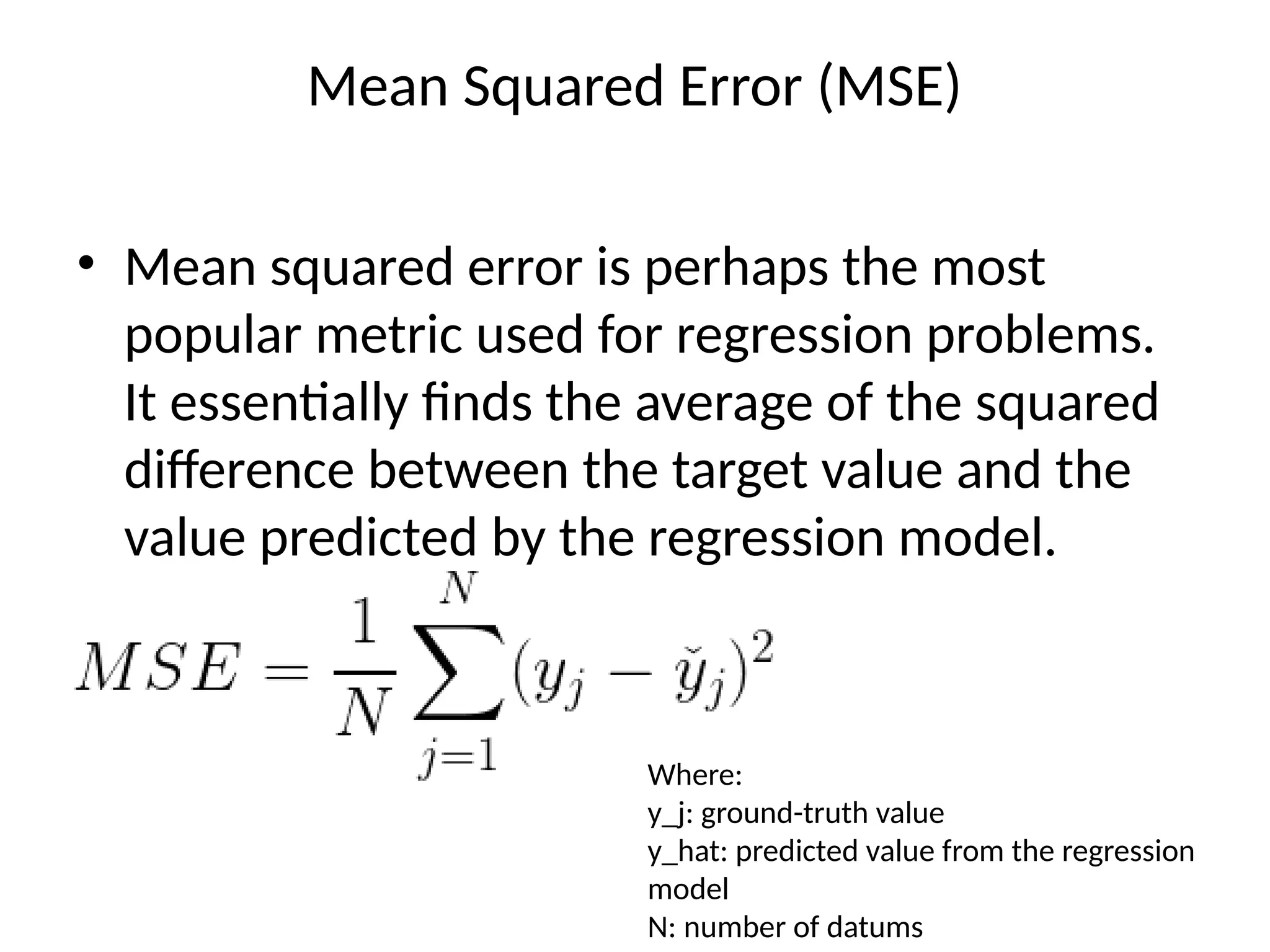
32. Mean Squared Error (MSE)
• Mean squared error is perhaps the most
popular metric used for regression problems.
It essentially finds the average of the squared
difference between the target value and the
value predicted by the regression model.
Where:
y_j: ground-truth value
y_hat: predicted value from the regression
model
N: number of datums

33. • It’s differentiable, so it can be optimized better.
• It penalizes even small errors by squaring them, which
essentially leads to an overestimation of how bad the
model is.
• Error interpretation has to be done with squaring
factor(scale) in mind. For example in our Boston
Housing regression problem, we got MSE=21.89 which
primarily corresponds to (Prices)².
• Due to the squaring factor, it’s fundamentally more
prone to outliers than other metrics.

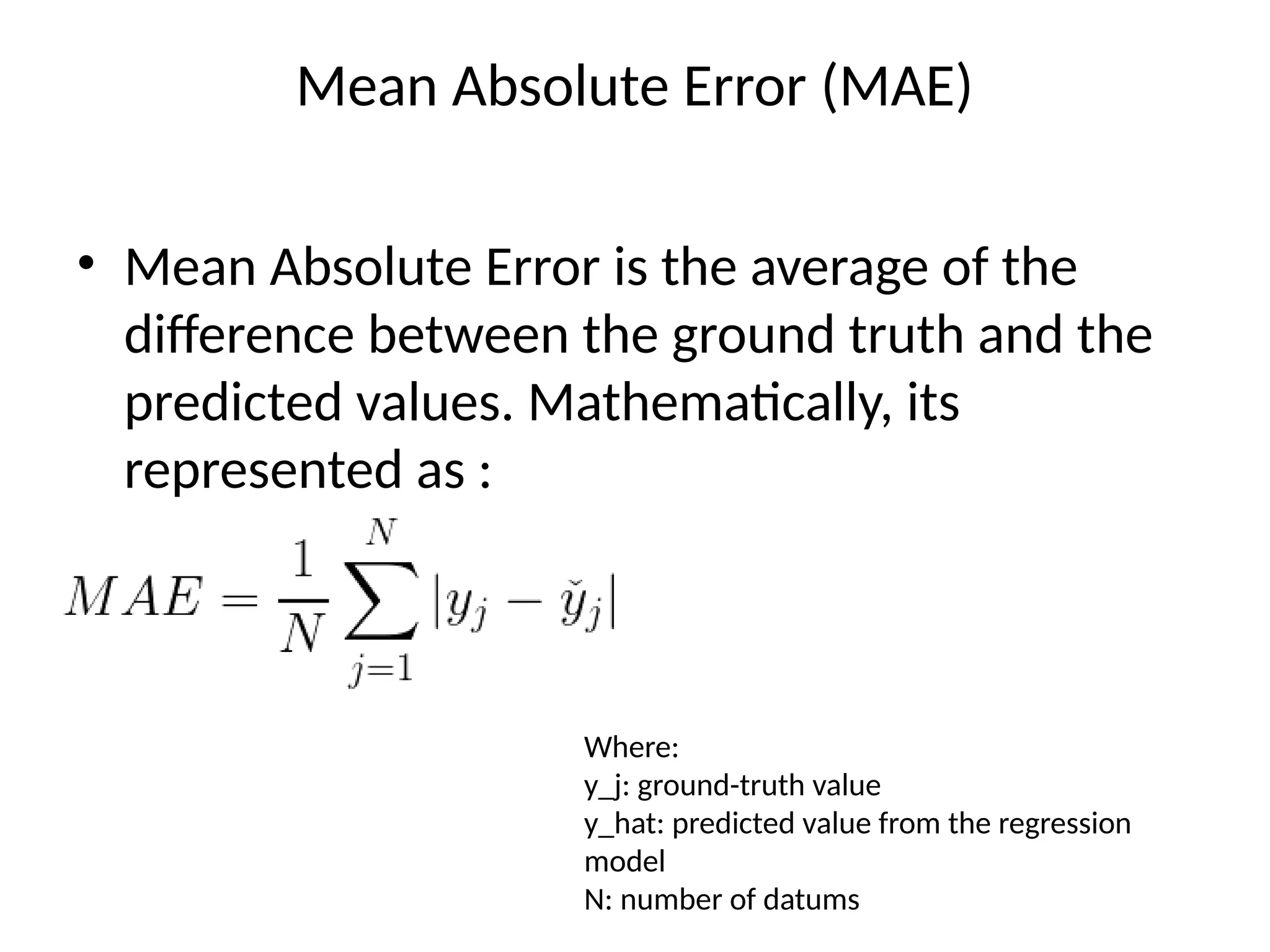
34. Mean Absolute Error (MAE)
• Mean Absolute Error is the average of the
difference between the ground truth and the
predicted values. Mathematically, its
represented as :
Where:
y_j: ground-truth value
y_hat: predicted value from the regression
model
N: number of datums

35. • It’s more robust towards outliers than MAE, since it
doesn’t exaggerate errors.
• It gives us a measure of how far the predictions were from
the actual output. However, since MAE uses absolute value
of the residual, it doesn’t give us an idea of the direction of
the error, i.e. whether we’re under-predicting or over-
predicting the data.
• Error interpretation needs no second thoughts, as it
perfectly aligns with the original degree of the variable.
• MAE is non-differentiable as opposed to MSE, which is
differentiable.

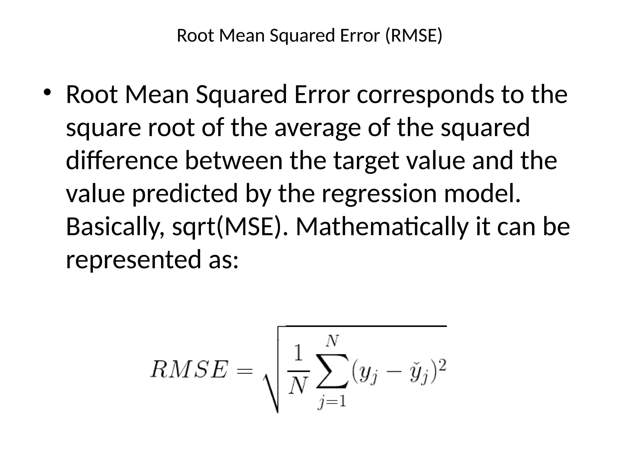
36. Root Mean Squared Error (RMSE)
• Root Mean Squared Error corresponds to the
square root of the average of the squared
difference between the target value and the
value predicted by the regression model.
Basically, sqrt(MSE). Mathematically it can be
represented as:

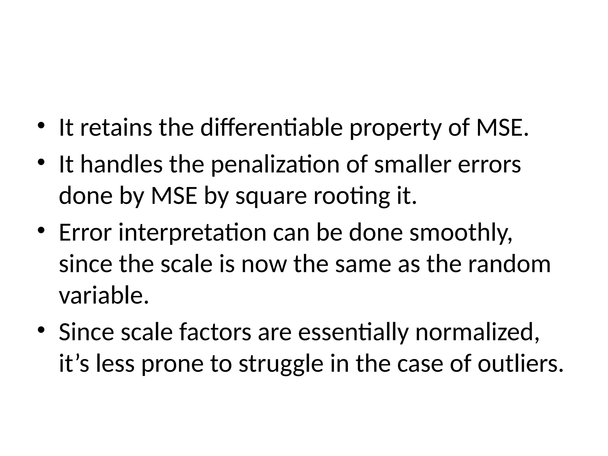
37. • It retains the differentiable property of MSE.
• It handles the penalization of smaller errors
done by MSE by square rooting it.
• Error interpretation can be done smoothly,
since the scale is now the same as the random
variable.
• Since scale factors are essentially normalized,
it’s less prone to struggle in the case of outliers.

38. R² Coefficient of determination
• R² Coefficient of determination actually works as a
post metric, meaning it’s a metric that’s calculated
using other metrics.
• The point of even calculating this coefficient is to
answer the question “How much (what %) of the
total variation in Y(target) is explained by the
variation in X(regression line)”
• This is calculated using the sum of squared errors.
Let’s go through the formulation to understand it
better.

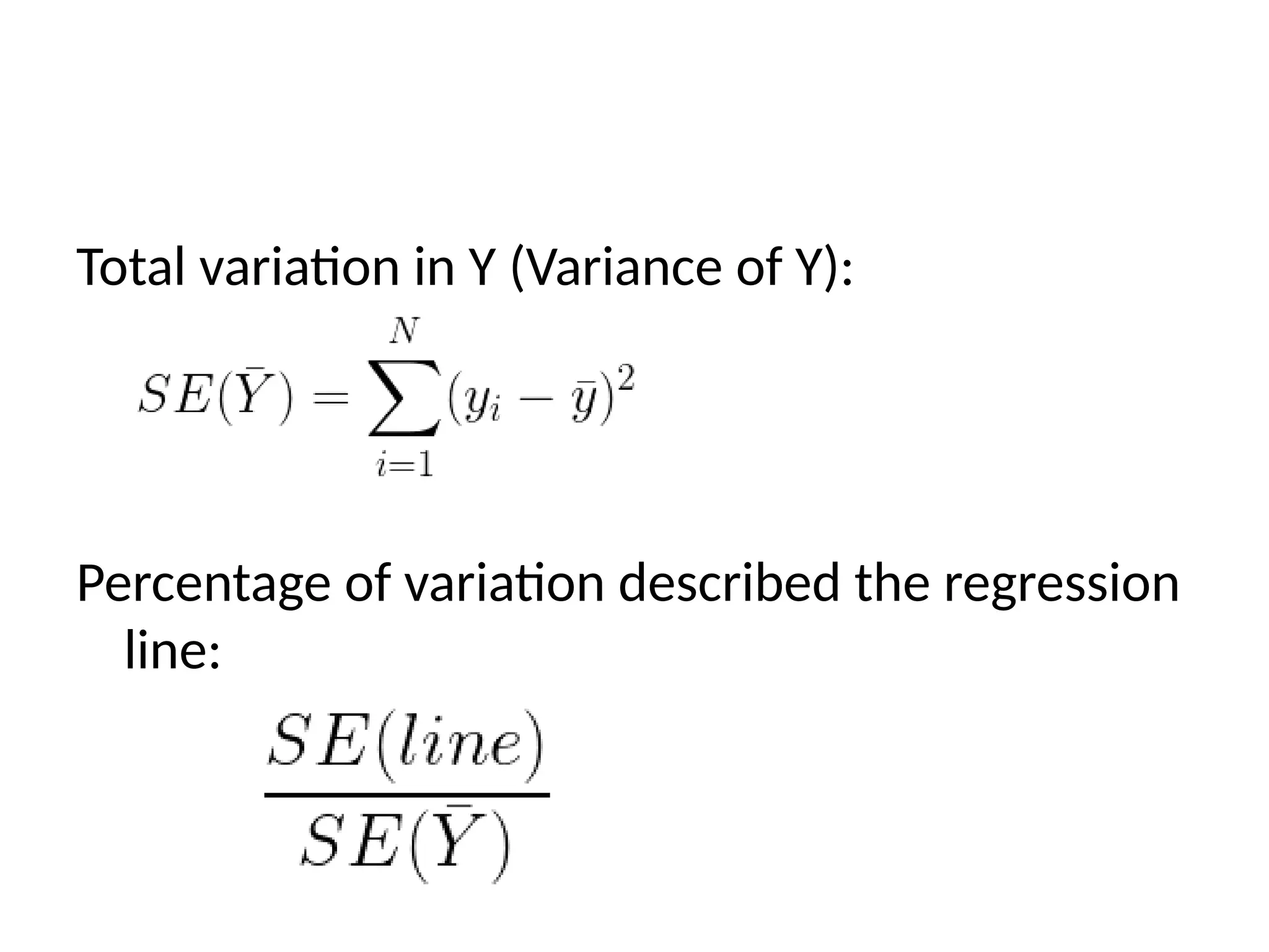
39. Total variation in Y (Variance of Y):
Percentage of variation described the regression
line:

40. the percentage of variation described the
regression line:
coefficient of determination, which can tell us
how good or bad the fit of the regression line
is:

41. • If the sum of Squared Error of the regression line is small =>
R² will be close to 1 (Ideal), meaning the regression was able
to capture 100% of the variance in the target variable.
• Conversely, if the sum of squared error of the regression line
is high => R² will be close to 0, meaning the regression wasn’t
able to capture any variance in the target variable.
• You might think that the range of R² is (0,1) but it’s actually (-
∞,1) because the ratio of squared errors of the regression
line and mean can surpass the value 1 if the squared error of
regression line is too high (>squared error of the mean).

42. • Micro and Macro Precision
• Micro and Macro Recalls
• Micro and Macro F-measure