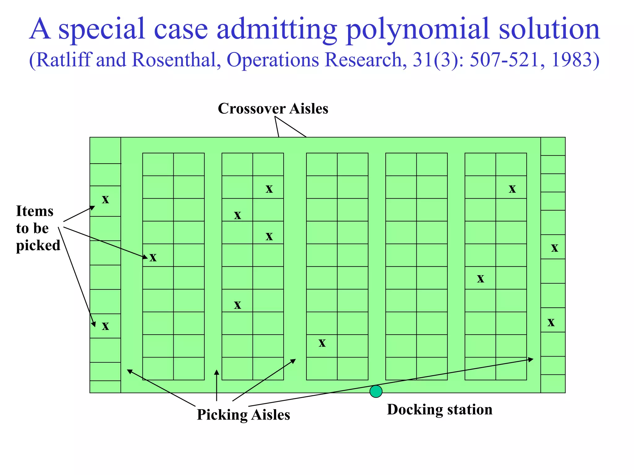
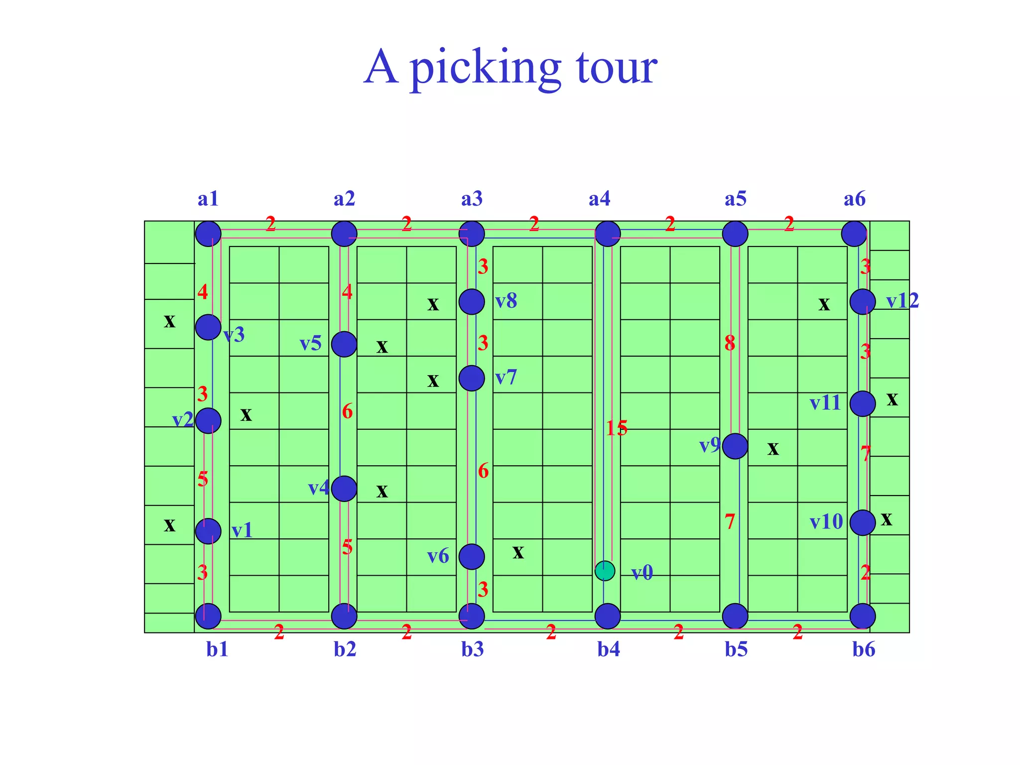
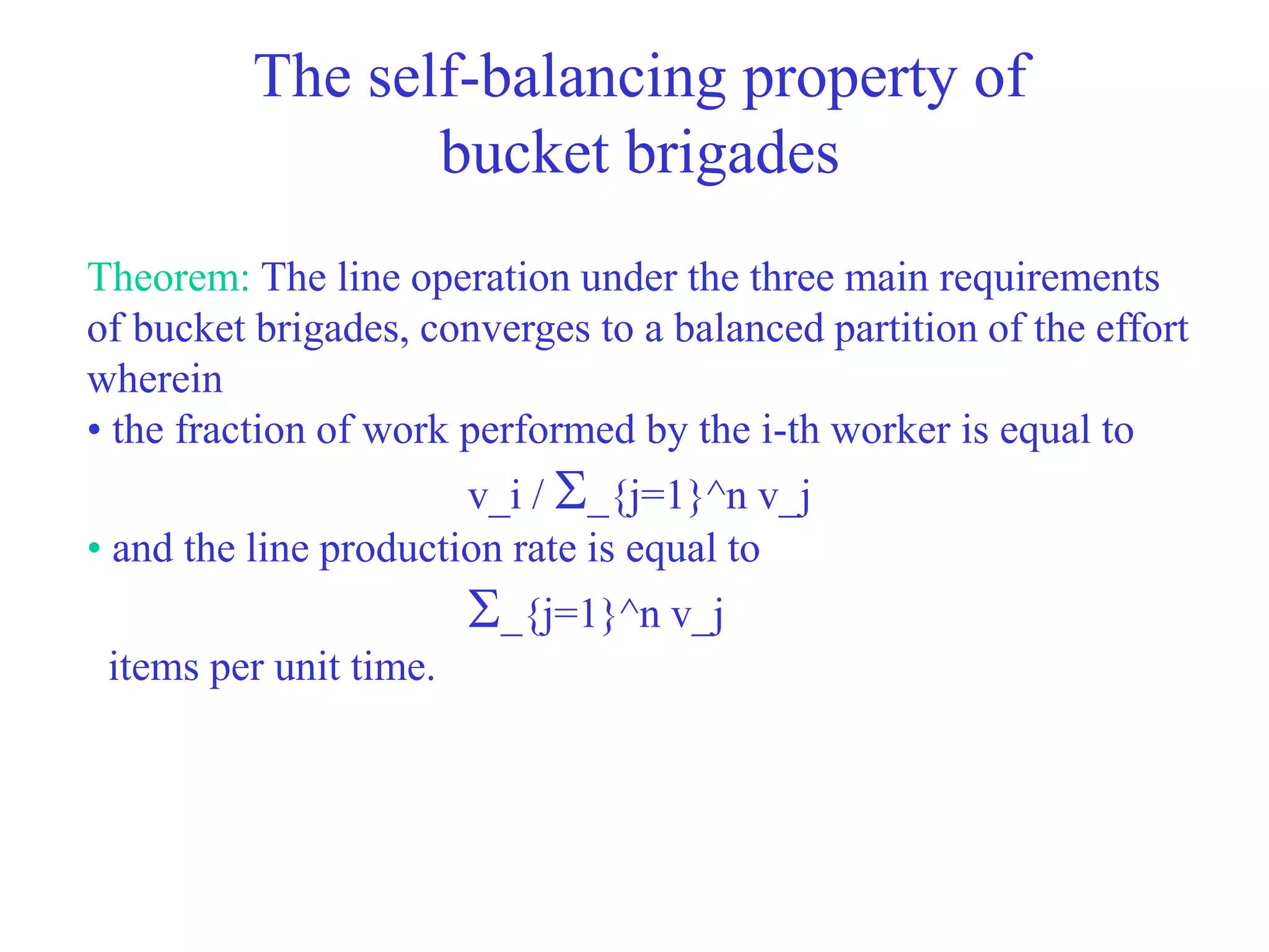
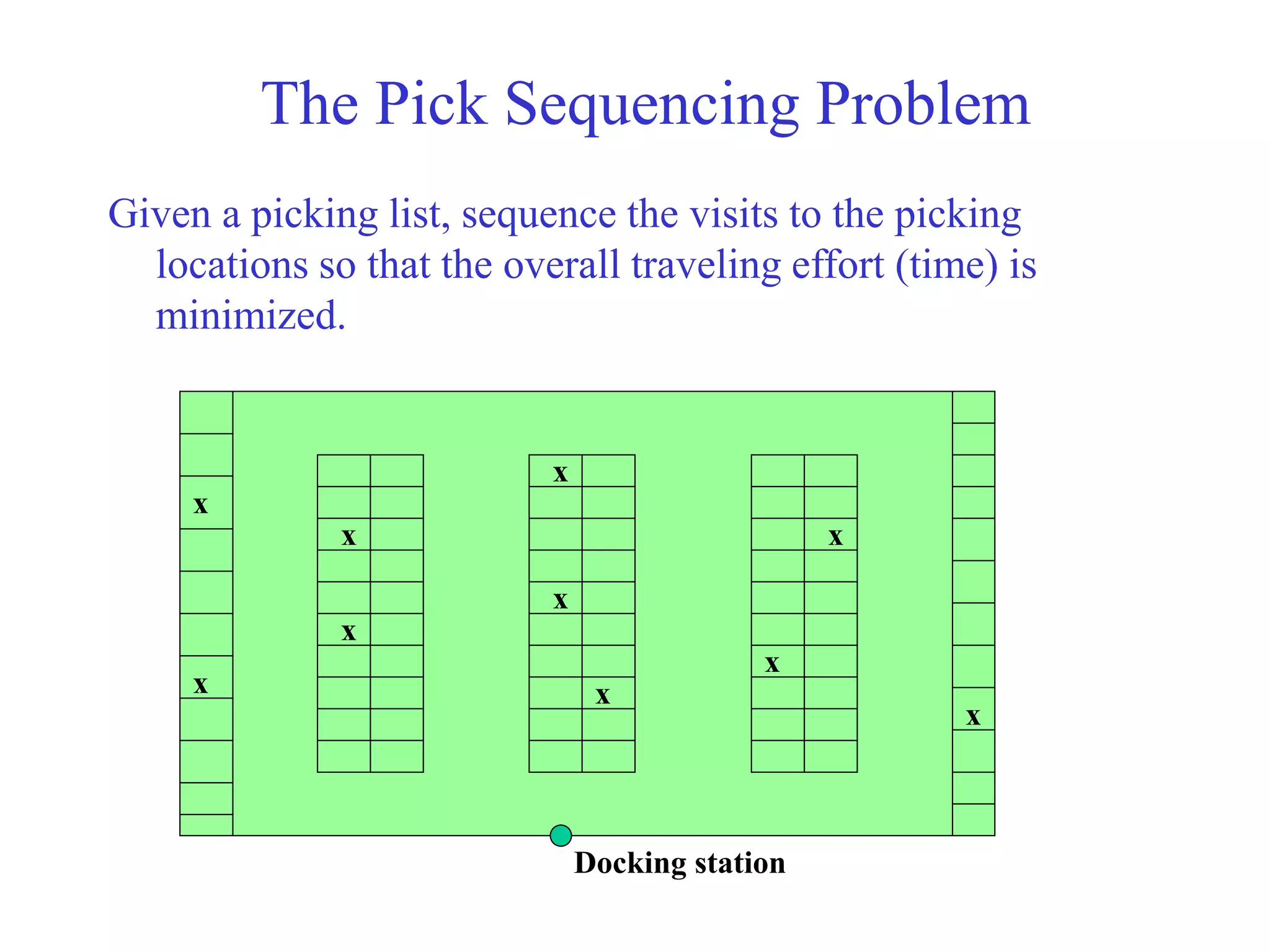
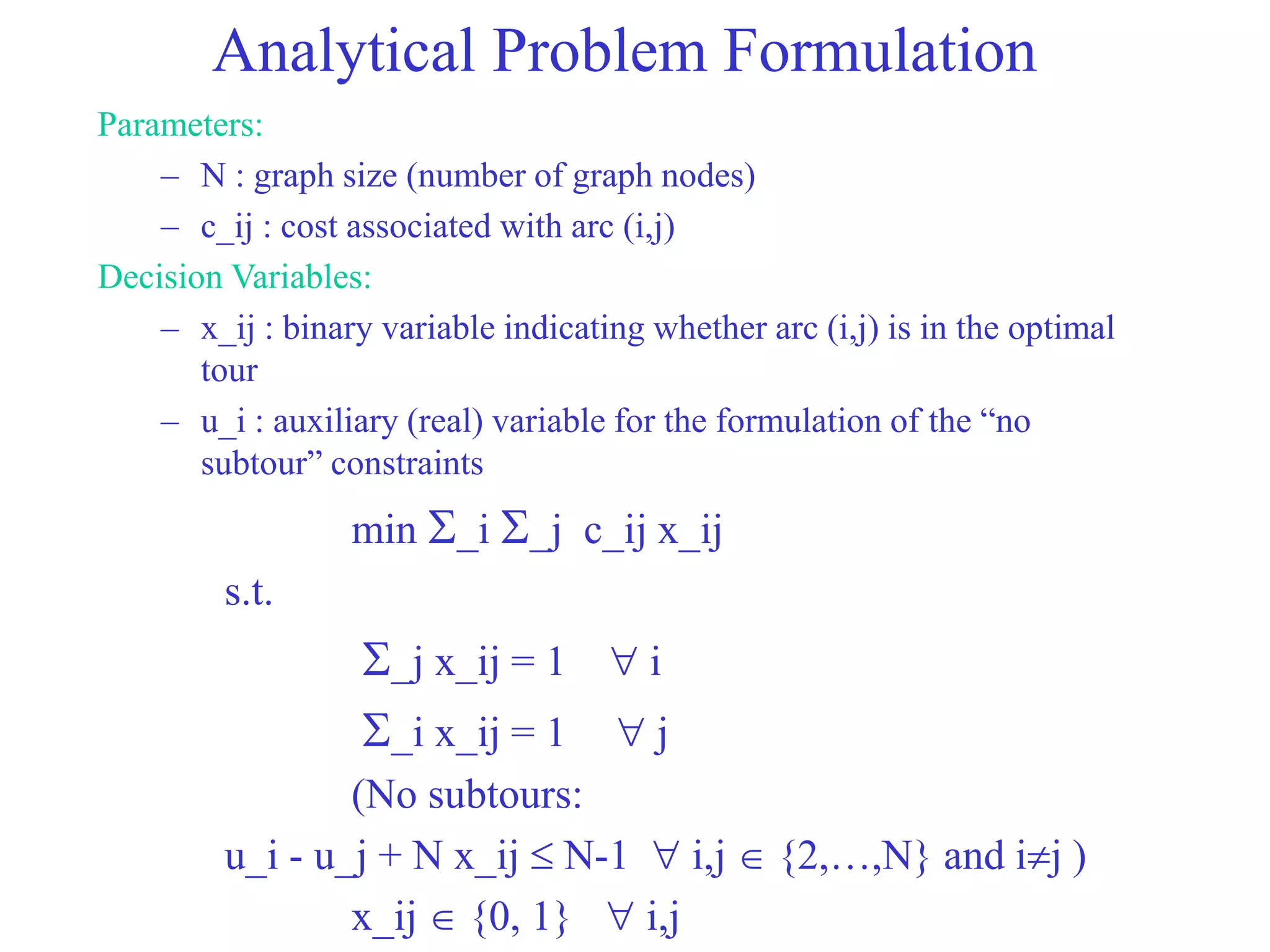
SlideShare a Scribd company logo
1 of 43
Order Picking Policies:
Pick Sequencing, Batching and
Zoning
The Pick Sequencing Problem
Given a picking list, sequence the visits to the picking
locations so that the overall traveling effort (time) is
minimized.
x
x
x
x
x
x
x
x
x
x
Docking station
Problem Abstraction:
The Traveling Salesman Problem (TSP)
Given a complete TSP graph:
1
2
3
4
5
c_ij
find a tour that visits all cities, with minimal total (traveling) cost;
e.g.:
1
2
3
4
5
<1, 2, 5, 3, 4>
Analytical Problem Formulation
Parameters:
– N : graph size (number of graph nodes)
– c_ij : cost associated with arc (i,j)
Decision Variables:
– x_ij : binary variable indicating whether arc (i,j) is in the optimal
tour
– u_i : auxiliary (real) variable for the formulation of the “no
subtour” constraints
min _i _j c_ij x_ij
s.t.
_j x_ij = 1  i
_i x_ij = 1  j
(No subtours:
u_i - u_j + N x_ij  N-1  i,j  {2,…,N} and ij )
x_ij  {0, 1}  i,j
Some remarks on the TSP problem and
its application in pick sequencing
• The TSP problem is an NP-complete problem: It can be solved
optimally for small instances, but in general, it will be solved through
heuristics.
• There is a vast literature on TSP and the development of heuristic
algorithms for it (e.g., Lawler, Lenstra, Rinnooy Kan and Shmoys,
“The Traveling Salesman Problem: A guided tour of combinatorial
optimization”, John Wiley and Sons, 1985).
• When the “no subtour” constraint is removed, the remaining
formulation defines a Linear Assignment Problem (LAP) (which is an
easy one; e.g., the “Hungarian Algorithm”) => Solving the
corresponding LAP can provide lower bounds for assessing the sub-
optimality of the solutions provided by the applied heuristics.
• In the considered application context, the distances c_ij should be
computed based on the appropriate distance metric; i.e., rectilinear,
Tchebychev, “shortest path”
The closest insertion algorithm:
A TSP heuristic (symmetric version)
Initialization:
S_p = <1>; S_a = {2,…,N}; c(j) = 1,  j  {2,…,N}; n=1;
While n < N do
n = n+1;
Selection step:
j* = argmin_{j  S_a} {c_{j,c(j)}};
S_a = S_a  {j*};
Insertion step:
i* = argmin_{i =1}^|S_p| {c_{[i],j*} + c_{j*,[i mod |S_p|+1]}
- c_{[i],[i mod |S_p|+1]}};
S_p = < [1],…,[i*], j*, [i*+1],…,[n]>;
 j  S_a, if c_{j,j*} < c_{j,c(j)} then c(j) = j*;
Remarks: 1. [i] denotes the node at i-th position of the constructed sub-tour.
2. If the distances are symmetric and satisfy the triangular inequality, the cost of
the solution provided by this heuristic is no worse than twice the optimal cost.
A special case admitting polynomial solution
(Ratliff and Rosenthal, Operations Research, 31(3): 507-521, 1983)
Docking station
Picking Aisles
Crossover Aisles
Items
to be
picked
x
x
x
x
x
x
x
x
x
x
x
x
A graph-based representation of the
underlying topology
x
x
x
x
x
x
x
x
x
x
x
x
b1 b2 b3 b4 b5 b6
a1 a2 a3 a4 a5 a6
v0
v1
v2
v3
v4
v5
v6
v7
v8
v9
v10
v11
v12
2
2
2 2 2
2
7
3
3
2 2 2
2 2
3
5
3
4 4
6
5
3
6
3
3
15
8
7
0
A picking tour
x
x
x
x
x
x
x
x
x
x
x
x
b1 b2 b3 b4 b5 b6
a1 a2 a3 a4 a5 a6
v0
v1
v2
v3
v4
v5
v6
v7
v8
v9
v10
v11
v12
2
2
2 2 2
2
7
3
3
2 2 2
2 2
3
5
3
4 4
6
5
3
6
3
3
15
8
7
Lj-, Aj and Lj+ sub-graphs, j=1,2,…,n
x
x
x
x
x
x
x
x
x
x
x
x
b1 b2 b3 b4 b5 b6
a1 a2 a3 a4 a5 a6
v0
v1
v2
v3
v4
v5
v6
v7
v8
v9
v10
v11
v12
2
2
2 2 2
2
7
3
3
2 2 2
2 2
3
5
3
4 4
6
5
3
6
3
3
15
8
7
Lj+ = Lj-  Aj
Lj(- or +) PTS (partial tour sub-graph)
x
x
x
x
x
x
x
x
x
x
x
x
b1 b2 b3 b4 b5 b6
a1 a2 a3 a4 a5 a6
v0
v1
v2
v3
v4
v5
v6
v7
v8
v9
v10
v11
v12
2
2
2 2 2
2
7
3
3
2 2 2
2 2
3
5
3
4 4
6
5
3
6
3
3
15
8
7
L3- PTS : (E, E, 2C)
L3+PTS: (U, U, 1C)
A key observation
The only possible characterizations for an Lj (- or +) PTS are the
following:
• (U, U, 1C)
• (0, E, 1C)
• (E, 0, 1C)
• (E, E, 1C)
• (E, E, 2C)
• (0, 0, 0C)
• (0, 0, 1C)
where the triplet (X, Y, Z) should be interpreted as follows:
• X (Y): degree parity for node a_j (b_j) - 0, Even, Uneven (odd)
• Z: number of connected components in Lj PTS, excluding the
vertices with zero degree
Going from Lj- to Lj+…
a_j a_j a_j
a_j a_j a_j
b_j b_j b_j b_j b_j b_j
(I-i) (I-ii) (I-iii) (I-iv) (I-v) (I-vi)
Going from Lj- to Lj+…(cont.)
Lj- class (I-i) (I-ii) (I-iii) (I-iv) (I-v) (I-vi)a
(U,U,1C) (E,E,1C) (U,U,1C) (U,U,1C) (U,U,1C) (U,U,1C) (U,U,1C)
(E,0,1C) (U,U,1C) (E,0,1C) (E,E,2C) (E,E,2C) (E,E,1C) (E,0,1C)
(0,E,1C) (U,U,1C) (E,E,2C) (0,E,1C) (E,E,2C) (E,E,1C) (0,E,1C)
(E,E,1C) (U,U,1C) (E,E,1C) (E,E,1C) (E,E,1C) (E,E,1C) (E,E,1C)
(E,E,2C) (U,U,1C) (E,E,2C) (E,E,2C) (E,E,2C) (E,E,1C) (E,E,2C)
(0,0,0C)b (U,U,1C) (E,0,1C) (0,E,1C) (E,E,2C) (E,E,1C) (0,0,0C)
(0,0,1C)c d (0,0,1C)
a: This is not a feasible configuration if there is any item to be picked in aisle j
b: This class can occur only if there are no items to be picked to the left of aisle j
c: This class is feasible only if there are no items to be picked to the right of aisle j
d: Could never be optimal
TABLE I
Going from Lj+ to L(j+1)-…
a_j+1
a_j
b_j b_j+1
a_j+1
a_j
b_j b_j+1
a_j+1
a_j
b_j b_j+1
a_j+1
a_j
b_j b_j+1
a_j+1
a_j
b_j b_j+1
(II-i) (II-ii) (II-iii)
(II-iv) (II-v)
Going from Lj+ to L(j+1)-…(cont.)
Lj+ class (II-i) (II-ii) (II-iii) (II-iv) (II-v)
(U,U,1C) (U,U,1C) a a a a
(E,0,1C) a (E,0,1C) b (E,E,2C) (0,0,1C)
(0,E,1C) a b (0,E,1C) (E,E,2C) (0,0,1C)
(E,E,1C) a (E,0,1C) (0,E,1C) (E,E,1C) (0,0,1C)
(E,E,2C) a b b (E,E,2C) b
(0,0,0C) c c c c (0,0,0C)
(0,0,1C) b b b b (0,0,1C)
a: The degrees of a_j and b_j are odd.
b: No completion can connect the graph.
c: Would never be optimal.
TABLE II
A polynomial-complexity algorithm for
computing a minimum-length tour
• Initialization: L1- PTS = null graph for every class type
• For <L1+, L2-, L2+,…,Ln-, Ln+)
– compute a minimum-length PTS for each of the seven
classes, using the minimum-length PTS’s constructed in
the previous stage, and the information provided in
Tables I and II.
– Remark: For case (I-iv), a minimum-length PTS is
obtained by putting the gap between the two adjacent
v_i’s in aisle j that are farthest apart.
• A minimum-length tour is defined by a minimum-
length Ln+ PTS.
Example (c.f., slide 8)
PTS-class L1- L1+ L2- L2+ L3- L3+
1.(U,U,1C) 15,-,I-I 19,1,II-I 37,1,I-iv 41,1,II-I 53,2,I-I
2.(E,0,1C) 24,-,I-ii 28,2,II-ii 48,2,I-ii 38,4,II-ii 62,2,I-ii
3.(0,E,1C) 22,-,I-iii 26,3,II-iii 48,3,I-iii 38,4,II-iii 62,3,I-iii
4.(E,E,1C) 30,-,I-v 38,4,II-iv 34,1,I-I 42,4,II-iv 56,1,I-I
5.(E,E,2C) 20,-,I-iv 28,5,II-iv 44,3,I-? 52,5,II-iv 56,2,I-iv
6.(0,0,0C)
7.(0,0,1C) 22,3,II-v 34,4,II-v
PTS-class L4- L4+ L5- L5+ L6- L6+
1.(U,U,1C) 57,1,II-I 57,1,I-iii 61,1,II-I 75,1,I-iii 79,1,II-I 95,1,I-iv
2.(E,0,1C) 60,4,II-ii 90,2,I-ii 68,4,II-ii 84,2,I-ii 80,4,II-ii 106,2,I-ii
3.(0,E,1C) 60,4,II-iii 60,3,I-iii 64,3,II-iii 78,2,I-iii 80,4,II-iii 104,3,I-iii
4.(E,E,1C) 64,4,II-iv 64,4,I-iii 72,4,II-iv 76,1,I-I 84,4,II-iv 94,1,I,I
5.(E,E,2C) 64,5,II-iv 60,2,I-iii 68,3,II-iv 80,3,I-ii 86,3,II-iv 96,2,I,iv
6.(0,0,0C)
7.(0,0,1C) 56,4,II-v 60,3,II-v 76,4,II-v
Example: The optimal tour
x
x
x
x
x
x
x
x
x
x
x
x
b1 b2 b3 b4 b5 b6
a1 a2 a3 a4 a5 a6
v0
v1
v2
v3
v4
v5
v6
v7
v8
v9
v10
v11
v12
2
2
2 2 2
2
7
3
3
2 2 2
2 2
3
5
3
4 4
6
5
3
6
3
3
15
8
7
0
k-STRIP: A computationally simple
heuristic for rectangular areas
x
x
x
x
x
x
x
x
x
x
I/O point
x
x
• When A is the unit square, an optimized k =  (n/2) , and for this value, the worst-
case tour length generated by the heuristic is between 1.075n and 1.414 n, for large n.
• The computational complexity is O(n logn).
• Supowit, Reingold and Plaisted, “The traveling salesman problem and minimum
matching in the unit square”, SIAM J. Computing, 12(1): 144-156, 1983.
The bin-numbering heuristic
(Bartholdi and Platzman, Material Flow, 4: 247-254, 1988)
• Basic idea: Number bins / storage locations in a way that
filling the orders by visiting the associated bins in
increasing numbers will lead to efficient routings.
• Advantages:
– Once the numbering is established, developing the order routes
becomes extremely simple.
– Easy to adjust routes dynamically upon the arrival of new orders.
• Basic underlying problem:
How do you establish good bin-numbering schemes?
Example of a numbering scheme
(Is it a good one?)
Order: {1, 10, 13, 28, 30, 44, 50, 62}
1
2
3
4
5
6
7
8
9 10
11
12
13
14
15
16 17
18
19
20 21 22
23
24
25 26
27
28
29
30
31
32 33 34
35
36 37
38
39
40
41
42
43
64
44
45
46
47
48
49
50 51 52
53
54 55
56
57
58
59
60
61
62
63
1 6
7
4
2 2
4
7
11
Resulting route length: 44 (using rectilinear distances of the cell
centroids)
An alternative numbering scheme
1 2
3
4
5 6
7
8
9 10
11
12
13
15
16 17 18
19
20
21 22
23
24
25 26
27
28
29 30
31
32 33 34
35
36
37
38
39 40
41
42
43
64
44
45 46
47
48 49 50
51
52
53 54
55
56
57 58
59
60
61 62
63
14
Order: {1,4,12,14,21,48,58,64}
1
1
4
2 2
4
7
4
7
Resulting route length: 32
Key concept: Space-filling curves
(see also http://www.isye.gatech.edu/faculty/John_Bartholdi/mow/mow.html)
• Closed curves that sweep the entire region while preserving nearness.
• Technically, they define a continuous mapping of the unit interval on the unit
square.
• Typical example: Sierpinski’s space-filling curve:
The Sierpinski space-filling curve
Applying the Sierpinski space-filling curve
in the previous bin-numbering example
1
2 3
4
5
6 7
8
9 10
11
12
13
15
16
17
18
19
20 21
22
23 24
25
26
27
28 29
30
31
32 33
34
35 36
37
38 39
40
41
42
43
64
44 45 46
47
48
49 50
51
52
53
54
55
56
57 58
59
60
61
62
63
14
Order: {1,2,13,17,18,32,46,52}
Resulting route length: 34
1
1
6
2
2
4
7
4
7
Some properties of the bin-numbering
schemes based on the Sierpinski
space-filling curve
• If n locations are to be visited throughout a warehouse of
area A, then the length of the retrieval route is at most
(2nA).
• If every location is equally likely to be visited, then on
average, the retrieval route produced by the corresponding
bin-numbering heuristic will be 25% longer than the
shortest possible route length.
• The above results have been derived using the Euclidean
metric for measuring the traveling distances, but they are
robust with respect to other metrics that preserve
“closeness” according to the Euclidean metric.
Characterizing the best bin-numbering
scheme...
• …is computationally very hard.
• Some good schemes can be obtained through interchange
techniques (e.g., 2 or 3-opt), where the efficiency of each of
the considered schemes is evaluated through simulation.
• The optimal bin-numbering scheme depends on:
– the underlying geometry of the picking facility
– the frequency with which the various storage locations are visited
(and therefore, the applying storage policy)
• In general, the logic underlying the utilization of the space-
filling curves is more useful / pertinent for storage areas with
small visitation frequencies for their locations.
• For areas with high visitation frequencies, numbering
schemes suggesting an exhaustive sweeping of the region
tend to perform better (c.f., Bartholdi & Platzman, pg. 252).
Bin-numbering in structures with
complicated geometry
When the considered area has a structure too complex to
measure traveling effort by Euclidean or a relative metric,
the logic underlying the application of space-filling curves
to bin-numbering can be applied in a hierarchical fashion:
• separate the entire area under consideration to smaller
areas of simpler geometry;
• design a numbering sequence for each of these areas using
the space-filling curve logic;
• develop a visiting sequence for the areas developed in step
1, by passing a space-filling curve among their I/O points.
Order Batching
(based on De Koster et. al., “Efficient
orderbatching methods in warehouses”, Inlt.
Jrnl of Prod. Res., Vol. 37, No. 7, pgs 1479-
1504, 1999)
Problem Description
• Given a set of orders, cluster them into batches - i.e.,
subsets of orders that are to be picked simultaneously by
one picker at a single trip - s.t.
– the total traveling distance / time is minimized
– while each batch does not exceed some measure of the
picker capacity (e.g., number of items / volume of the
resulting batch, number of distinct orders in a batch)
• Theoretically, the problem can be solved by:
– enumerating all feasible partitions of the given order set into
batches;
– evaluating the total traveling distance / time for each partition;
– picking the partition with the smallest traveling distance / time.
• However, combinatorial explosion of partitions =>
heuristics
Order-Batching Heuristics
Naive Intelligent
FCFS Seed Algorithms Savings Algorithms
(Batches are built
sequentially, one at
a time)
(All batches are built
simultaneously, by
merging partially
developed batches)
(Orders are clustered
based on the sequence
of their appearance)
The generic structure for seed algorithms
• While there are unprocessed orders,
– Pick a new seed order according to some seed selection
rule;
– while there are unprocessed orders and the batch has
not reached the imposed capacity limit
• pick a new order to be added to the batch according
to an order addition rule;
• add the selected order to the batch, provided that the
imposed capacity limit is not violated;
• (update the batch seed to the union of the previous
batch seed and the new order)
Typical seed selection rules
• Random selection
• the order with the farthest item (w.r.t. the shipping station)
• the order with the largest number of aisles to be visited
• the order with the largest aisle range (absolute difference
between the most left aisle number and the most right aisle
number to be visited)
• the order with the largest number of items
• the order with the longest travel time
• Remark: If the batch seed is updated after every order
addition, the algorithm is characterized as dynamic or
cumulative mode; ow., it is said to be static or single mode.
Typical order addition rules
• Time saving: choose the order that, together with the batch seed,
ensures the largest time saving compared with the individual picking
of the two orders.
• Choose the order that minimizes the number of additional aisles,
compared to the seed order, that have to be visited by the resulting
batch route.
• Choose the order for which the absolute difference between the order’s
center of gravity (COG) and the COG of the batch seed is the smallest;
COG is the weighted average aisle number of the order, with the aisle
weights defined by the number of items in the aisle.
• Choose the order with the property that the sum of distances* between
every item of the seed and the closest item in the order is minimized.
• * distances must be measured by an appropriately selected metric
The (standard) savings algorithm
• Initialization: B: = order set (each order defines its own batch)
• Repeat
– For each pair (i,j) in the current batch set B
• compute the time savings s_ij = t_i + t_j - t_ij, where t_i/j is
the time required for picking batch i/j and t_ij is the time
required for picking the batch resulting from the merging of
batches i and j.
– Rank batch pairs (i,j) in decreasing s_ij.
– Pick the first batch pair (i,j) in the ranked list, for which the
merging of its constituent batches does not violate the imposed
capacity limit, and merge batches i and j: B := (B-{i,j}) U {i+j}
until no further batch merging is possible.
• Remark: The algorithm result depends on the adopted pick sequencing
rule.
Some findings regarding the (relative)
performance of the presented batch
algorithms (De Koster et. al.)
• Intelligent batching leads to significant improvements compared to
single-order picking and naïve batching schemes.
• In seed algorithms, dynamic seed definition leads to better
performance than static seed definition.
• The best seed selection rules are focusing on orders dispersed over a
large number of aisles and involving long travel times.
• The best order addition rules (c.f. corresponding slide) tend also to be
the most robust (i.e., they yield the best results in all warehouse
configurations considered in the simulation).
• Savings algorithms have good performance, in general, but they tend
to be computationally more expensive than seed algorithms.
• The performance of the applied batching algorithm has a significant
dependence on the adopted pick sequencing rule.
• The largest the number of orders per batch (the batch capacity limit),
the smaller the savings from intelligent batching (and therefore,
simpler batching schemes become more eligible candidates)
Warehouse Zoning
The two main concepts of zoning in
contemporary warehousing
Warehouse zoning: The physical and/or logical segmentation
of the warehouse / picking area, through
– the employment of different storage modes and
practices due to the product differentiation w.r.t.
• dimensions,
• physical characteristics
• storage and material handling requirements
• throughput,
• etc.
– the parallelization of the order-picking activity.
Zone-based order picking
Progressive Zoning / Order assembly
Parallel/Simultaneous Zoning (typically organized in pick-waves with
downstream sortation)
Order
To packing and shipping
Z1 Z2 Z3 Z4 Z5
Order (Batch)
To sorting and consolidation
Z1 Z2 Z3 Z4 Z5
Defining effective zones for order-picking
• Main objective: Try to achieve maximum utilization of the
picking resources, by distributing “equally” the total
(picking) workload among the defined zones.
• However, the warehouse picking environment usually is a
very dynamic environment; workload profiles are
constantly changing.
• Existing zoning systems seek to balance the average
workloads across zones, based on some hypothetical order
work-content and worker behavioral models.
• Furthermore, constant zone redefinition requires a lot of
effort from, both, the warehouse management (who must
keep track of all the workload changes and re-establish the
zones) and the warehouse pickers (who must adjust to the
new policies).
• Very limited scientific literature.
Bucket Brigades
( c.f. Bartholdi & Hackman, Chpt. 10)
• A dynamic self-balancing scheme for progressive zoning.
• The three main requirements of bucket brigades:
– Carry work forward, from station to station, until
someone takes over your work.
– If a worker catches up to his successor, he remains idle
until the station is available (i.e., no overpassing is
allowed)
– Workers are sequenced from slowest to fastest.
The self-balancing property of
bucket brigades
Theorem: The line operation under the three main requirements
of bucket brigades, converges to a balanced partition of the effort
wherein
• the fraction of work performed by the i-th worker is equal to
v_i / _{j=1}^n v_j
• and the line production rate is equal to
_{j=1}^n v_j
items per unit time.

More Related Content

Similar to Order-Picking-Policies.ppt

Clustering and Factorization using Apache SystemML by Alexandre V Evfimievski
Clustering and Factorization using Apache SystemML by  Alexandre V EvfimievskiClustering and Factorization using Apache SystemML by  Alexandre V Evfimievski
Clustering and Factorization using Apache SystemML by Alexandre V EvfimievskiArvind Surve
 
Unit-2 raster scan graphics,line,circle and polygon algorithms
Unit-2 raster scan graphics,line,circle and polygon algorithmsUnit-2 raster scan graphics,line,circle and polygon algorithms
Unit-2 raster scan graphics,line,circle and polygon algorithmsAmol Gaikwad
 
Open GL 04 linealgos
Open GL 04 linealgosOpen GL 04 linealgos
Open GL 04 linealgosRoziq Bahtiar
 
Applied Algorithms and Structures week999
Applied Algorithms and Structures week999Applied Algorithms and Structures week999
Applied Algorithms and Structures week999fashiontrendzz20
 
Tall-and-skinny Matrix Computations in MapReduce (ICME MR 2013)
Tall-and-skinny Matrix Computations in MapReduce (ICME MR 2013)Tall-and-skinny Matrix Computations in MapReduce (ICME MR 2013)
Tall-and-skinny Matrix Computations in MapReduce (ICME MR 2013)Austin Benson
 
Algorithms - "Chapter 2 getting started"
Algorithms - "Chapter 2 getting started"Algorithms - "Chapter 2 getting started"
Algorithms - "Chapter 2 getting started"Ra'Fat Al-Msie'deen
 
Line drawing algorithm and antialiasing techniques
Line drawing algorithm and antialiasing techniquesLine drawing algorithm and antialiasing techniques
Line drawing algorithm and antialiasing techniquesAnkit Garg
 
unit-4-dynamic programming
unit-4-dynamic programmingunit-4-dynamic programming
unit-4-dynamic programminghodcsencet
 
Add math may june 2016 p1
Add math may june 2016 p1Add math may june 2016 p1
Add math may june 2016 p1Don Cunningham
 
Branch and bounding : Data structures
Branch and bounding : Data structuresBranch and bounding : Data structures
Branch and bounding : Data structuresKàŕtheek Jåvvàjí
 
SYSTEM IDENTIFICATION USING CEREBELLAR MODEL ARITHMETIC COMPUTER
SYSTEM IDENTIFICATION USING CEREBELLAR MODEL ARITHMETIC COMPUTERSYSTEM IDENTIFICATION USING CEREBELLAR MODEL ARITHMETIC COMPUTER
SYSTEM IDENTIFICATION USING CEREBELLAR MODEL ARITHMETIC COMPUTERTarun Kumar
 

Similar to Order-Picking-Policies.ppt (20)

Clustering and Factorization using Apache SystemML by Alexandre V Evfimievski
Clustering and Factorization using Apache SystemML by  Alexandre V EvfimievskiClustering and Factorization using Apache SystemML by  Alexandre V Evfimievski
Clustering and Factorization using Apache SystemML by Alexandre V Evfimievski
 
Clustering and Factorization using Apache SystemML by Alexandre V Evfimievski
Clustering and Factorization using Apache SystemML by  Alexandre V EvfimievskiClustering and Factorization using Apache SystemML by  Alexandre V Evfimievski
Clustering and Factorization using Apache SystemML by Alexandre V Evfimievski
 
Unit-2 raster scan graphics,line,circle and polygon algorithms
Unit-2 raster scan graphics,line,circle and polygon algorithmsUnit-2 raster scan graphics,line,circle and polygon algorithms
Unit-2 raster scan graphics,line,circle and polygon algorithms
 
Dip mcq1
Dip mcq1Dip mcq1
Dip mcq1
 
Computer graphics 2
Computer graphics 2Computer graphics 2
Computer graphics 2
 
Chap08alg
Chap08algChap08alg
Chap08alg
 
Chap08alg
Chap08algChap08alg
Chap08alg
 
Primitives
PrimitivesPrimitives
Primitives
 
Open GL 04 linealgos
Open GL 04 linealgosOpen GL 04 linealgos
Open GL 04 linealgos
 
Ijetcas14 567
Ijetcas14 567Ijetcas14 567
Ijetcas14 567
 
Applied Algorithms and Structures week999
Applied Algorithms and Structures week999Applied Algorithms and Structures week999
Applied Algorithms and Structures week999
 
Tall-and-skinny Matrix Computations in MapReduce (ICME MR 2013)
Tall-and-skinny Matrix Computations in MapReduce (ICME MR 2013)Tall-and-skinny Matrix Computations in MapReduce (ICME MR 2013)
Tall-and-skinny Matrix Computations in MapReduce (ICME MR 2013)
 
Algorithms - "Chapter 2 getting started"
Algorithms - "Chapter 2 getting started"Algorithms - "Chapter 2 getting started"
Algorithms - "Chapter 2 getting started"
 
Line drawing algorithm and antialiasing techniques
Line drawing algorithm and antialiasing techniquesLine drawing algorithm and antialiasing techniques
Line drawing algorithm and antialiasing techniques
 
CG-Lecture3.pptx
CG-Lecture3.pptxCG-Lecture3.pptx
CG-Lecture3.pptx
 
2_1 Edit Distance.pptx
2_1 Edit Distance.pptx2_1 Edit Distance.pptx
2_1 Edit Distance.pptx
 
unit-4-dynamic programming
unit-4-dynamic programmingunit-4-dynamic programming
unit-4-dynamic programming
 
Add math may june 2016 p1
Add math may june 2016 p1Add math may june 2016 p1
Add math may june 2016 p1
 
Branch and bounding : Data structures
Branch and bounding : Data structuresBranch and bounding : Data structures
Branch and bounding : Data structures
 
SYSTEM IDENTIFICATION USING CEREBELLAR MODEL ARITHMETIC COMPUTER
SYSTEM IDENTIFICATION USING CEREBELLAR MODEL ARITHMETIC COMPUTERSYSTEM IDENTIFICATION USING CEREBELLAR MODEL ARITHMETIC COMPUTER
SYSTEM IDENTIFICATION USING CEREBELLAR MODEL ARITHMETIC COMPUTER
 

Recently uploaded

BEST ✨ Call Girls In Shangri-La Eros New Delhi✔️ 9871031762 ✔️ Escorts Servic...
BEST ✨ Call Girls In Shangri-La Eros New Delhi✔️ 9871031762 ✔️ Escorts Servic...BEST ✨ Call Girls In Shangri-La Eros New Delhi✔️ 9871031762 ✔️ Escorts Servic...
BEST ✨ Call Girls In Shangri-La Eros New Delhi✔️ 9871031762 ✔️ Escorts Servic...noida100girls
 
BEST ✨ Call Girls In Greater Noida ✔️ 9871031762 ✔️ Escorts Service In Delhi ...
BEST ✨ Call Girls In Greater Noida ✔️ 9871031762 ✔️ Escorts Service In Delhi ...BEST ✨ Call Girls In Greater Noida ✔️ 9871031762 ✔️ Escorts Service In Delhi ...
BEST ✨ Call Girls In Greater Noida ✔️ 9871031762 ✔️ Escorts Service In Delhi ...noida100girls
 
Maya❤️Call girls in Mohali ☎️7435815124☎️ Call Girl service in Mohali☎️ Mohal...
Maya❤️Call girls in Mohali ☎️7435815124☎️ Call Girl service in Mohali☎️ Mohal...Maya❤️Call girls in Mohali ☎️7435815124☎️ Call Girl service in Mohali☎️ Mohal...
Maya❤️Call girls in Mohali ☎️7435815124☎️ Call Girl service in Mohali☎️ Mohal...Sheetaleventcompany
 
Call girls in Jaipur 9358660226 escort service in Jaipur
Call girls in Jaipur 9358660226 escort service in JaipurCall girls in Jaipur 9358660226 escort service in Jaipur
Call girls in Jaipur 9358660226 escort service in Jaipurrahul222jai
 
BEST ✨ Call Girls In MG Road Gurgaon ✔️ 9871031762 ✔️ Escorts Service In De...
BEST ✨ Call Girls In  MG Road Gurgaon  ✔️ 9871031762 ✔️ Escorts Service In De...BEST ✨ Call Girls In  MG Road Gurgaon  ✔️ 9871031762 ✔️ Escorts Service In De...
BEST ✨ Call Girls In MG Road Gurgaon ✔️ 9871031762 ✔️ Escorts Service In De...noida100girls
 
Best VIP Call Girls Noida Sector 63 Call Me: 8448380779
Best VIP Call Girls Noida Sector 63 Call Me: 8448380779Best VIP Call Girls Noida Sector 63 Call Me: 8448380779
Best VIP Call Girls Noida Sector 63 Call Me: 8448380779Delhi Call girls
 
BEST ✨ Call Girls In Noida Electronic City ✔️ 9871031762 ✔️ Escorts Service I...
BEST ✨ Call Girls In Noida Electronic City ✔️ 9871031762 ✔️ Escorts Service I...BEST ✨ Call Girls In Noida Electronic City ✔️ 9871031762 ✔️ Escorts Service I...
BEST ✨ Call Girls In Noida Electronic City ✔️ 9871031762 ✔️ Escorts Service I...noida100girls
 
Russian ​❤️ Call Girls In Malviya Nagar ✔️9773824855✔️ Escorts Service In Del...
Russian ​❤️ Call Girls In Malviya Nagar ✔️9773824855✔️ Escorts Service In Del...Russian ​❤️ Call Girls In Malviya Nagar ✔️9773824855✔️ Escorts Service In Del...
Russian ​❤️ Call Girls In Malviya Nagar ✔️9773824855✔️ Escorts Service In Del...noida100girls
 
Best VIP Call Girls Noida Sector 49 Call Me: 8448380779
Best VIP Call Girls Noida Sector 49 Call Me: 8448380779Best VIP Call Girls Noida Sector 49 Call Me: 8448380779
Best VIP Call Girls Noida Sector 49 Call Me: 8448380779Delhi Call girls
 
Best VIP Call Girls Noida Sector 62 Call Me: 8448380779
Best VIP Call Girls Noida Sector 62 Call Me: 8448380779Best VIP Call Girls Noida Sector 62 Call Me: 8448380779
Best VIP Call Girls Noida Sector 62 Call Me: 8448380779Delhi Call girls
 
Russian ​❤️ Call Girls In Radisson Blu MBD Hotel, Noida ✔️ 9871031762 ✔️ Esco...
Russian ​❤️ Call Girls In Radisson Blu MBD Hotel, Noida ✔️ 9871031762 ✔️ Esco...Russian ​❤️ Call Girls In Radisson Blu MBD Hotel, Noida ✔️ 9871031762 ✔️ Esco...
Russian ​❤️ Call Girls In Radisson Blu MBD Hotel, Noida ✔️ 9871031762 ✔️ Esco...noida100girls
 
Cheap Rate ➥8448380779 ▻Call Girls In Sector 57 Gurgaon
Cheap Rate ➥8448380779 ▻Call Girls In Sector 57 GurgaonCheap Rate ➥8448380779 ▻Call Girls In Sector 57 Gurgaon
Cheap Rate ➥8448380779 ▻Call Girls In Sector 57 GurgaonDelhi Call girls
 
BEST ✨Call Girls In Park Plaza Gurugram ✔️9773824855✔️ Escorts Service In Del...
BEST ✨Call Girls In Park Plaza Gurugram ✔️9773824855✔️ Escorts Service In Del...BEST ✨Call Girls In Park Plaza Gurugram ✔️9773824855✔️ Escorts Service In Del...
BEST ✨Call Girls In Park Plaza Gurugram ✔️9773824855✔️ Escorts Service In Del...noida100girls
 
CALL ON ➥8923113531 🔝Call Girls Vikas Nagar Lucknow best Female service 🧥
CALL ON ➥8923113531 🔝Call Girls Vikas Nagar Lucknow best Female service  🧥CALL ON ➥8923113531 🔝Call Girls Vikas Nagar Lucknow best Female service  🧥
CALL ON ➥8923113531 🔝Call Girls Vikas Nagar Lucknow best Female service 🧥anilsa9823
 
Call Girls In Hauz Khas Delhi 9654467111 Independent Escorts Service
Call Girls In Hauz Khas Delhi 9654467111 Independent Escorts ServiceCall Girls In Hauz Khas Delhi 9654467111 Independent Escorts Service
Call Girls In Hauz Khas Delhi 9654467111 Independent Escorts ServiceSapana Sha
 
CALL ON ➥8923113531 🔝Call Girls Kakori Lucknow best sexual service
CALL ON ➥8923113531 🔝Call Girls Kakori Lucknow best sexual serviceCALL ON ➥8923113531 🔝Call Girls Kakori Lucknow best sexual service
CALL ON ➥8923113531 🔝Call Girls Kakori Lucknow best sexual serviceanilsa9823
 
BEST ✨ Call Girls In Park Plaza Faridabad ✔️ 9871031762 ✔️ Escorts Service In...
BEST ✨ Call Girls In Park Plaza Faridabad ✔️ 9871031762 ✔️ Escorts Service In...BEST ✨ Call Girls In Park Plaza Faridabad ✔️ 9871031762 ✔️ Escorts Service In...
BEST ✨ Call Girls In Park Plaza Faridabad ✔️ 9871031762 ✔️ Escorts Service In...noida100girls
 
Russian ​❤️ Call Girls In The Grand New Delhi Near By Vasant Kunj ✔️ 9871031...
Russian ​❤️ Call Girls In The Grand New Delhi Near By Vasant Kunj  ✔️ 9871031...Russian ​❤️ Call Girls In The Grand New Delhi Near By Vasant Kunj  ✔️ 9871031...
Russian ​❤️ Call Girls In The Grand New Delhi Near By Vasant Kunj ✔️ 9871031...noida100girls
 

Recently uploaded (18)

BEST ✨ Call Girls In Shangri-La Eros New Delhi✔️ 9871031762 ✔️ Escorts Servic...
BEST ✨ Call Girls In Shangri-La Eros New Delhi✔️ 9871031762 ✔️ Escorts Servic...BEST ✨ Call Girls In Shangri-La Eros New Delhi✔️ 9871031762 ✔️ Escorts Servic...
BEST ✨ Call Girls In Shangri-La Eros New Delhi✔️ 9871031762 ✔️ Escorts Servic...
 
BEST ✨ Call Girls In Greater Noida ✔️ 9871031762 ✔️ Escorts Service In Delhi ...
BEST ✨ Call Girls In Greater Noida ✔️ 9871031762 ✔️ Escorts Service In Delhi ...BEST ✨ Call Girls In Greater Noida ✔️ 9871031762 ✔️ Escorts Service In Delhi ...
BEST ✨ Call Girls In Greater Noida ✔️ 9871031762 ✔️ Escorts Service In Delhi ...
 
Maya❤️Call girls in Mohali ☎️7435815124☎️ Call Girl service in Mohali☎️ Mohal...
Maya❤️Call girls in Mohali ☎️7435815124☎️ Call Girl service in Mohali☎️ Mohal...Maya❤️Call girls in Mohali ☎️7435815124☎️ Call Girl service in Mohali☎️ Mohal...
Maya❤️Call girls in Mohali ☎️7435815124☎️ Call Girl service in Mohali☎️ Mohal...
 
Call girls in Jaipur 9358660226 escort service in Jaipur
Call girls in Jaipur 9358660226 escort service in JaipurCall girls in Jaipur 9358660226 escort service in Jaipur
Call girls in Jaipur 9358660226 escort service in Jaipur
 
BEST ✨ Call Girls In MG Road Gurgaon ✔️ 9871031762 ✔️ Escorts Service In De...
BEST ✨ Call Girls In  MG Road Gurgaon  ✔️ 9871031762 ✔️ Escorts Service In De...BEST ✨ Call Girls In  MG Road Gurgaon  ✔️ 9871031762 ✔️ Escorts Service In De...
BEST ✨ Call Girls In MG Road Gurgaon ✔️ 9871031762 ✔️ Escorts Service In De...
 
Best VIP Call Girls Noida Sector 63 Call Me: 8448380779
Best VIP Call Girls Noida Sector 63 Call Me: 8448380779Best VIP Call Girls Noida Sector 63 Call Me: 8448380779
Best VIP Call Girls Noida Sector 63 Call Me: 8448380779
 
BEST ✨ Call Girls In Noida Electronic City ✔️ 9871031762 ✔️ Escorts Service I...
BEST ✨ Call Girls In Noida Electronic City ✔️ 9871031762 ✔️ Escorts Service I...BEST ✨ Call Girls In Noida Electronic City ✔️ 9871031762 ✔️ Escorts Service I...
BEST ✨ Call Girls In Noida Electronic City ✔️ 9871031762 ✔️ Escorts Service I...
 
Russian ​❤️ Call Girls In Malviya Nagar ✔️9773824855✔️ Escorts Service In Del...
Russian ​❤️ Call Girls In Malviya Nagar ✔️9773824855✔️ Escorts Service In Del...Russian ​❤️ Call Girls In Malviya Nagar ✔️9773824855✔️ Escorts Service In Del...
Russian ​❤️ Call Girls In Malviya Nagar ✔️9773824855✔️ Escorts Service In Del...
 
Best VIP Call Girls Noida Sector 49 Call Me: 8448380779
Best VIP Call Girls Noida Sector 49 Call Me: 8448380779Best VIP Call Girls Noida Sector 49 Call Me: 8448380779
Best VIP Call Girls Noida Sector 49 Call Me: 8448380779
 
Best VIP Call Girls Noida Sector 62 Call Me: 8448380779
Best VIP Call Girls Noida Sector 62 Call Me: 8448380779Best VIP Call Girls Noida Sector 62 Call Me: 8448380779
Best VIP Call Girls Noida Sector 62 Call Me: 8448380779
 
Russian ​❤️ Call Girls In Radisson Blu MBD Hotel, Noida ✔️ 9871031762 ✔️ Esco...
Russian ​❤️ Call Girls In Radisson Blu MBD Hotel, Noida ✔️ 9871031762 ✔️ Esco...Russian ​❤️ Call Girls In Radisson Blu MBD Hotel, Noida ✔️ 9871031762 ✔️ Esco...
Russian ​❤️ Call Girls In Radisson Blu MBD Hotel, Noida ✔️ 9871031762 ✔️ Esco...
 
Cheap Rate ➥8448380779 ▻Call Girls In Sector 57 Gurgaon
Cheap Rate ➥8448380779 ▻Call Girls In Sector 57 GurgaonCheap Rate ➥8448380779 ▻Call Girls In Sector 57 Gurgaon
Cheap Rate ➥8448380779 ▻Call Girls In Sector 57 Gurgaon
 
BEST ✨Call Girls In Park Plaza Gurugram ✔️9773824855✔️ Escorts Service In Del...
BEST ✨Call Girls In Park Plaza Gurugram ✔️9773824855✔️ Escorts Service In Del...BEST ✨Call Girls In Park Plaza Gurugram ✔️9773824855✔️ Escorts Service In Del...
BEST ✨Call Girls In Park Plaza Gurugram ✔️9773824855✔️ Escorts Service In Del...
 
CALL ON ➥8923113531 🔝Call Girls Vikas Nagar Lucknow best Female service 🧥
CALL ON ➥8923113531 🔝Call Girls Vikas Nagar Lucknow best Female service  🧥CALL ON ➥8923113531 🔝Call Girls Vikas Nagar Lucknow best Female service  🧥
CALL ON ➥8923113531 🔝Call Girls Vikas Nagar Lucknow best Female service 🧥
 
Call Girls In Hauz Khas Delhi 9654467111 Independent Escorts Service
Call Girls In Hauz Khas Delhi 9654467111 Independent Escorts ServiceCall Girls In Hauz Khas Delhi 9654467111 Independent Escorts Service
Call Girls In Hauz Khas Delhi 9654467111 Independent Escorts Service
 
CALL ON ➥8923113531 🔝Call Girls Kakori Lucknow best sexual service
CALL ON ➥8923113531 🔝Call Girls Kakori Lucknow best sexual serviceCALL ON ➥8923113531 🔝Call Girls Kakori Lucknow best sexual service
CALL ON ➥8923113531 🔝Call Girls Kakori Lucknow best sexual service
 
BEST ✨ Call Girls In Park Plaza Faridabad ✔️ 9871031762 ✔️ Escorts Service In...
BEST ✨ Call Girls In Park Plaza Faridabad ✔️ 9871031762 ✔️ Escorts Service In...BEST ✨ Call Girls In Park Plaza Faridabad ✔️ 9871031762 ✔️ Escorts Service In...
BEST ✨ Call Girls In Park Plaza Faridabad ✔️ 9871031762 ✔️ Escorts Service In...
 
Russian ​❤️ Call Girls In The Grand New Delhi Near By Vasant Kunj ✔️ 9871031...
Russian ​❤️ Call Girls In The Grand New Delhi Near By Vasant Kunj  ✔️ 9871031...Russian ​❤️ Call Girls In The Grand New Delhi Near By Vasant Kunj  ✔️ 9871031...
Russian ​❤️ Call Girls In The Grand New Delhi Near By Vasant Kunj ✔️ 9871031...
 

Order-Picking-Policies.ppt

  • 1. Order Picking Policies: Pick Sequencing, Batching and Zoning
  • 2. The Pick Sequencing Problem Given a picking list, sequence the visits to the picking locations so that the overall traveling effort (time) is minimized. x x x x x x x x x x Docking station
  • 3. Problem Abstraction: The Traveling Salesman Problem (TSP) Given a complete TSP graph: 1 2 3 4 5 c_ij find a tour that visits all cities, with minimal total (traveling) cost; e.g.: 1 2 3 4 5 <1, 2, 5, 3, 4>
  • 4. Analytical Problem Formulation Parameters: – N : graph size (number of graph nodes) – c_ij : cost associated with arc (i,j) Decision Variables: – x_ij : binary variable indicating whether arc (i,j) is in the optimal tour – u_i : auxiliary (real) variable for the formulation of the “no subtour” constraints min _i _j c_ij x_ij s.t. _j x_ij = 1  i _i x_ij = 1  j (No subtours: u_i - u_j + N x_ij  N-1  i,j  {2,…,N} and ij ) x_ij  {0, 1}  i,j
  • 5. Some remarks on the TSP problem and its application in pick sequencing • The TSP problem is an NP-complete problem: It can be solved optimally for small instances, but in general, it will be solved through heuristics. • There is a vast literature on TSP and the development of heuristic algorithms for it (e.g., Lawler, Lenstra, Rinnooy Kan and Shmoys, “The Traveling Salesman Problem: A guided tour of combinatorial optimization”, John Wiley and Sons, 1985). • When the “no subtour” constraint is removed, the remaining formulation defines a Linear Assignment Problem (LAP) (which is an easy one; e.g., the “Hungarian Algorithm”) => Solving the corresponding LAP can provide lower bounds for assessing the sub- optimality of the solutions provided by the applied heuristics. • In the considered application context, the distances c_ij should be computed based on the appropriate distance metric; i.e., rectilinear, Tchebychev, “shortest path”
  • 6. The closest insertion algorithm: A TSP heuristic (symmetric version) Initialization: S_p = <1>; S_a = {2,…,N}; c(j) = 1,  j  {2,…,N}; n=1; While n < N do n = n+1; Selection step: j* = argmin_{j  S_a} {c_{j,c(j)}}; S_a = S_a {j*}; Insertion step: i* = argmin_{i =1}^|S_p| {c_{[i],j*} + c_{j*,[i mod |S_p|+1]} - c_{[i],[i mod |S_p|+1]}}; S_p = < [1],…,[i*], j*, [i*+1],…,[n]>;  j  S_a, if c_{j,j*} < c_{j,c(j)} then c(j) = j*; Remarks: 1. [i] denotes the node at i-th position of the constructed sub-tour. 2. If the distances are symmetric and satisfy the triangular inequality, the cost of the solution provided by this heuristic is no worse than twice the optimal cost.
  • 7. A special case admitting polynomial solution (Ratliff and Rosenthal, Operations Research, 31(3): 507-521, 1983) Docking station Picking Aisles Crossover Aisles Items to be picked x x x x x x x x x x x x
  • 8. A graph-based representation of the underlying topology x x x x x x x x x x x x b1 b2 b3 b4 b5 b6 a1 a2 a3 a4 a5 a6 v0 v1 v2 v3 v4 v5 v6 v7 v8 v9 v10 v11 v12 2 2 2 2 2 2 7 3 3 2 2 2 2 2 3 5 3 4 4 6 5 3 6 3 3 15 8 7 0
  • 9. A picking tour x x x x x x x x x x x x b1 b2 b3 b4 b5 b6 a1 a2 a3 a4 a5 a6 v0 v1 v2 v3 v4 v5 v6 v7 v8 v9 v10 v11 v12 2 2 2 2 2 2 7 3 3 2 2 2 2 2 3 5 3 4 4 6 5 3 6 3 3 15 8 7
  • 10. Lj-, Aj and Lj+ sub-graphs, j=1,2,…,n x x x x x x x x x x x x b1 b2 b3 b4 b5 b6 a1 a2 a3 a4 a5 a6 v0 v1 v2 v3 v4 v5 v6 v7 v8 v9 v10 v11 v12 2 2 2 2 2 2 7 3 3 2 2 2 2 2 3 5 3 4 4 6 5 3 6 3 3 15 8 7 Lj+ = Lj-  Aj
  • 11. Lj(- or +) PTS (partial tour sub-graph) x x x x x x x x x x x x b1 b2 b3 b4 b5 b6 a1 a2 a3 a4 a5 a6 v0 v1 v2 v3 v4 v5 v6 v7 v8 v9 v10 v11 v12 2 2 2 2 2 2 7 3 3 2 2 2 2 2 3 5 3 4 4 6 5 3 6 3 3 15 8 7 L3- PTS : (E, E, 2C) L3+PTS: (U, U, 1C)
  • 12. A key observation The only possible characterizations for an Lj (- or +) PTS are the following: • (U, U, 1C) • (0, E, 1C) • (E, 0, 1C) • (E, E, 1C) • (E, E, 2C) • (0, 0, 0C) • (0, 0, 1C) where the triplet (X, Y, Z) should be interpreted as follows: • X (Y): degree parity for node a_j (b_j) - 0, Even, Uneven (odd) • Z: number of connected components in Lj PTS, excluding the vertices with zero degree
  • 13. Going from Lj- to Lj+… a_j a_j a_j a_j a_j a_j b_j b_j b_j b_j b_j b_j (I-i) (I-ii) (I-iii) (I-iv) (I-v) (I-vi)
  • 14. Going from Lj- to Lj+…(cont.) Lj- class (I-i) (I-ii) (I-iii) (I-iv) (I-v) (I-vi)a (U,U,1C) (E,E,1C) (U,U,1C) (U,U,1C) (U,U,1C) (U,U,1C) (U,U,1C) (E,0,1C) (U,U,1C) (E,0,1C) (E,E,2C) (E,E,2C) (E,E,1C) (E,0,1C) (0,E,1C) (U,U,1C) (E,E,2C) (0,E,1C) (E,E,2C) (E,E,1C) (0,E,1C) (E,E,1C) (U,U,1C) (E,E,1C) (E,E,1C) (E,E,1C) (E,E,1C) (E,E,1C) (E,E,2C) (U,U,1C) (E,E,2C) (E,E,2C) (E,E,2C) (E,E,1C) (E,E,2C) (0,0,0C)b (U,U,1C) (E,0,1C) (0,E,1C) (E,E,2C) (E,E,1C) (0,0,0C) (0,0,1C)c d (0,0,1C) a: This is not a feasible configuration if there is any item to be picked in aisle j b: This class can occur only if there are no items to be picked to the left of aisle j c: This class is feasible only if there are no items to be picked to the right of aisle j d: Could never be optimal TABLE I
  • 15. Going from Lj+ to L(j+1)-… a_j+1 a_j b_j b_j+1 a_j+1 a_j b_j b_j+1 a_j+1 a_j b_j b_j+1 a_j+1 a_j b_j b_j+1 a_j+1 a_j b_j b_j+1 (II-i) (II-ii) (II-iii) (II-iv) (II-v)
  • 16. Going from Lj+ to L(j+1)-…(cont.) Lj+ class (II-i) (II-ii) (II-iii) (II-iv) (II-v) (U,U,1C) (U,U,1C) a a a a (E,0,1C) a (E,0,1C) b (E,E,2C) (0,0,1C) (0,E,1C) a b (0,E,1C) (E,E,2C) (0,0,1C) (E,E,1C) a (E,0,1C) (0,E,1C) (E,E,1C) (0,0,1C) (E,E,2C) a b b (E,E,2C) b (0,0,0C) c c c c (0,0,0C) (0,0,1C) b b b b (0,0,1C) a: The degrees of a_j and b_j are odd. b: No completion can connect the graph. c: Would never be optimal. TABLE II
  • 17. A polynomial-complexity algorithm for computing a minimum-length tour • Initialization: L1- PTS = null graph for every class type • For <L1+, L2-, L2+,…,Ln-, Ln+) – compute a minimum-length PTS for each of the seven classes, using the minimum-length PTS’s constructed in the previous stage, and the information provided in Tables I and II. – Remark: For case (I-iv), a minimum-length PTS is obtained by putting the gap between the two adjacent v_i’s in aisle j that are farthest apart. • A minimum-length tour is defined by a minimum- length Ln+ PTS.
  • 18. Example (c.f., slide 8) PTS-class L1- L1+ L2- L2+ L3- L3+ 1.(U,U,1C) 15,-,I-I 19,1,II-I 37,1,I-iv 41,1,II-I 53,2,I-I 2.(E,0,1C) 24,-,I-ii 28,2,II-ii 48,2,I-ii 38,4,II-ii 62,2,I-ii 3.(0,E,1C) 22,-,I-iii 26,3,II-iii 48,3,I-iii 38,4,II-iii 62,3,I-iii 4.(E,E,1C) 30,-,I-v 38,4,II-iv 34,1,I-I 42,4,II-iv 56,1,I-I 5.(E,E,2C) 20,-,I-iv 28,5,II-iv 44,3,I-? 52,5,II-iv 56,2,I-iv 6.(0,0,0C) 7.(0,0,1C) 22,3,II-v 34,4,II-v PTS-class L4- L4+ L5- L5+ L6- L6+ 1.(U,U,1C) 57,1,II-I 57,1,I-iii 61,1,II-I 75,1,I-iii 79,1,II-I 95,1,I-iv 2.(E,0,1C) 60,4,II-ii 90,2,I-ii 68,4,II-ii 84,2,I-ii 80,4,II-ii 106,2,I-ii 3.(0,E,1C) 60,4,II-iii 60,3,I-iii 64,3,II-iii 78,2,I-iii 80,4,II-iii 104,3,I-iii 4.(E,E,1C) 64,4,II-iv 64,4,I-iii 72,4,II-iv 76,1,I-I 84,4,II-iv 94,1,I,I 5.(E,E,2C) 64,5,II-iv 60,2,I-iii 68,3,II-iv 80,3,I-ii 86,3,II-iv 96,2,I,iv 6.(0,0,0C) 7.(0,0,1C) 56,4,II-v 60,3,II-v 76,4,II-v
  • 19. Example: The optimal tour x x x x x x x x x x x x b1 b2 b3 b4 b5 b6 a1 a2 a3 a4 a5 a6 v0 v1 v2 v3 v4 v5 v6 v7 v8 v9 v10 v11 v12 2 2 2 2 2 2 7 3 3 2 2 2 2 2 3 5 3 4 4 6 5 3 6 3 3 15 8 7 0
  • 20. k-STRIP: A computationally simple heuristic for rectangular areas x x x x x x x x x x I/O point x x • When A is the unit square, an optimized k =  (n/2) , and for this value, the worst- case tour length generated by the heuristic is between 1.075n and 1.414 n, for large n. • The computational complexity is O(n logn). • Supowit, Reingold and Plaisted, “The traveling salesman problem and minimum matching in the unit square”, SIAM J. Computing, 12(1): 144-156, 1983.
  • 21. The bin-numbering heuristic (Bartholdi and Platzman, Material Flow, 4: 247-254, 1988) • Basic idea: Number bins / storage locations in a way that filling the orders by visiting the associated bins in increasing numbers will lead to efficient routings. • Advantages: – Once the numbering is established, developing the order routes becomes extremely simple. – Easy to adjust routes dynamically upon the arrival of new orders. • Basic underlying problem: How do you establish good bin-numbering schemes?
  • 22. Example of a numbering scheme (Is it a good one?) Order: {1, 10, 13, 28, 30, 44, 50, 62} 1 2 3 4 5 6 7 8 9 10 11 12 13 14 15 16 17 18 19 20 21 22 23 24 25 26 27 28 29 30 31 32 33 34 35 36 37 38 39 40 41 42 43 64 44 45 46 47 48 49 50 51 52 53 54 55 56 57 58 59 60 61 62 63 1 6 7 4 2 2 4 7 11 Resulting route length: 44 (using rectilinear distances of the cell centroids)
  • 23. An alternative numbering scheme 1 2 3 4 5 6 7 8 9 10 11 12 13 15 16 17 18 19 20 21 22 23 24 25 26 27 28 29 30 31 32 33 34 35 36 37 38 39 40 41 42 43 64 44 45 46 47 48 49 50 51 52 53 54 55 56 57 58 59 60 61 62 63 14 Order: {1,4,12,14,21,48,58,64} 1 1 4 2 2 4 7 4 7 Resulting route length: 32
  • 24. Key concept: Space-filling curves (see also http://www.isye.gatech.edu/faculty/John_Bartholdi/mow/mow.html) • Closed curves that sweep the entire region while preserving nearness. • Technically, they define a continuous mapping of the unit interval on the unit square. • Typical example: Sierpinski’s space-filling curve:
  • 26. Applying the Sierpinski space-filling curve in the previous bin-numbering example 1 2 3 4 5 6 7 8 9 10 11 12 13 15 16 17 18 19 20 21 22 23 24 25 26 27 28 29 30 31 32 33 34 35 36 37 38 39 40 41 42 43 64 44 45 46 47 48 49 50 51 52 53 54 55 56 57 58 59 60 61 62 63 14 Order: {1,2,13,17,18,32,46,52} Resulting route length: 34 1 1 6 2 2 4 7 4 7
  • 27. Some properties of the bin-numbering schemes based on the Sierpinski space-filling curve • If n locations are to be visited throughout a warehouse of area A, then the length of the retrieval route is at most (2nA). • If every location is equally likely to be visited, then on average, the retrieval route produced by the corresponding bin-numbering heuristic will be 25% longer than the shortest possible route length. • The above results have been derived using the Euclidean metric for measuring the traveling distances, but they are robust with respect to other metrics that preserve “closeness” according to the Euclidean metric.
  • 28. Characterizing the best bin-numbering scheme... • …is computationally very hard. • Some good schemes can be obtained through interchange techniques (e.g., 2 or 3-opt), where the efficiency of each of the considered schemes is evaluated through simulation. • The optimal bin-numbering scheme depends on: – the underlying geometry of the picking facility – the frequency with which the various storage locations are visited (and therefore, the applying storage policy) • In general, the logic underlying the utilization of the space- filling curves is more useful / pertinent for storage areas with small visitation frequencies for their locations. • For areas with high visitation frequencies, numbering schemes suggesting an exhaustive sweeping of the region tend to perform better (c.f., Bartholdi & Platzman, pg. 252).
  • 29. Bin-numbering in structures with complicated geometry When the considered area has a structure too complex to measure traveling effort by Euclidean or a relative metric, the logic underlying the application of space-filling curves to bin-numbering can be applied in a hierarchical fashion: • separate the entire area under consideration to smaller areas of simpler geometry; • design a numbering sequence for each of these areas using the space-filling curve logic; • develop a visiting sequence for the areas developed in step 1, by passing a space-filling curve among their I/O points.
  • 30. Order Batching (based on De Koster et. al., “Efficient orderbatching methods in warehouses”, Inlt. Jrnl of Prod. Res., Vol. 37, No. 7, pgs 1479- 1504, 1999)
  • 31. Problem Description • Given a set of orders, cluster them into batches - i.e., subsets of orders that are to be picked simultaneously by one picker at a single trip - s.t. – the total traveling distance / time is minimized – while each batch does not exceed some measure of the picker capacity (e.g., number of items / volume of the resulting batch, number of distinct orders in a batch) • Theoretically, the problem can be solved by: – enumerating all feasible partitions of the given order set into batches; – evaluating the total traveling distance / time for each partition; – picking the partition with the smallest traveling distance / time. • However, combinatorial explosion of partitions => heuristics
  • 32. Order-Batching Heuristics Naive Intelligent FCFS Seed Algorithms Savings Algorithms (Batches are built sequentially, one at a time) (All batches are built simultaneously, by merging partially developed batches) (Orders are clustered based on the sequence of their appearance)
  • 33. The generic structure for seed algorithms • While there are unprocessed orders, – Pick a new seed order according to some seed selection rule; – while there are unprocessed orders and the batch has not reached the imposed capacity limit • pick a new order to be added to the batch according to an order addition rule; • add the selected order to the batch, provided that the imposed capacity limit is not violated; • (update the batch seed to the union of the previous batch seed and the new order)
  • 34. Typical seed selection rules • Random selection • the order with the farthest item (w.r.t. the shipping station) • the order with the largest number of aisles to be visited • the order with the largest aisle range (absolute difference between the most left aisle number and the most right aisle number to be visited) • the order with the largest number of items • the order with the longest travel time • Remark: If the batch seed is updated after every order addition, the algorithm is characterized as dynamic or cumulative mode; ow., it is said to be static or single mode.
  • 35. Typical order addition rules • Time saving: choose the order that, together with the batch seed, ensures the largest time saving compared with the individual picking of the two orders. • Choose the order that minimizes the number of additional aisles, compared to the seed order, that have to be visited by the resulting batch route. • Choose the order for which the absolute difference between the order’s center of gravity (COG) and the COG of the batch seed is the smallest; COG is the weighted average aisle number of the order, with the aisle weights defined by the number of items in the aisle. • Choose the order with the property that the sum of distances* between every item of the seed and the closest item in the order is minimized. • * distances must be measured by an appropriately selected metric
  • 36. The (standard) savings algorithm • Initialization: B: = order set (each order defines its own batch) • Repeat – For each pair (i,j) in the current batch set B • compute the time savings s_ij = t_i + t_j - t_ij, where t_i/j is the time required for picking batch i/j and t_ij is the time required for picking the batch resulting from the merging of batches i and j. – Rank batch pairs (i,j) in decreasing s_ij. – Pick the first batch pair (i,j) in the ranked list, for which the merging of its constituent batches does not violate the imposed capacity limit, and merge batches i and j: B := (B-{i,j}) U {i+j} until no further batch merging is possible. • Remark: The algorithm result depends on the adopted pick sequencing rule.
  • 37. Some findings regarding the (relative) performance of the presented batch algorithms (De Koster et. al.) • Intelligent batching leads to significant improvements compared to single-order picking and naïve batching schemes. • In seed algorithms, dynamic seed definition leads to better performance than static seed definition. • The best seed selection rules are focusing on orders dispersed over a large number of aisles and involving long travel times. • The best order addition rules (c.f. corresponding slide) tend also to be the most robust (i.e., they yield the best results in all warehouse configurations considered in the simulation). • Savings algorithms have good performance, in general, but they tend to be computationally more expensive than seed algorithms. • The performance of the applied batching algorithm has a significant dependence on the adopted pick sequencing rule. • The largest the number of orders per batch (the batch capacity limit), the smaller the savings from intelligent batching (and therefore, simpler batching schemes become more eligible candidates)
  • 39. The two main concepts of zoning in contemporary warehousing Warehouse zoning: The physical and/or logical segmentation of the warehouse / picking area, through – the employment of different storage modes and practices due to the product differentiation w.r.t. • dimensions, • physical characteristics • storage and material handling requirements • throughput, • etc. – the parallelization of the order-picking activity.
  • 40. Zone-based order picking Progressive Zoning / Order assembly Parallel/Simultaneous Zoning (typically organized in pick-waves with downstream sortation) Order To packing and shipping Z1 Z2 Z3 Z4 Z5 Order (Batch) To sorting and consolidation Z1 Z2 Z3 Z4 Z5
  • 41. Defining effective zones for order-picking • Main objective: Try to achieve maximum utilization of the picking resources, by distributing “equally” the total (picking) workload among the defined zones. • However, the warehouse picking environment usually is a very dynamic environment; workload profiles are constantly changing. • Existing zoning systems seek to balance the average workloads across zones, based on some hypothetical order work-content and worker behavioral models. • Furthermore, constant zone redefinition requires a lot of effort from, both, the warehouse management (who must keep track of all the workload changes and re-establish the zones) and the warehouse pickers (who must adjust to the new policies). • Very limited scientific literature.
  • 42. Bucket Brigades ( c.f. Bartholdi & Hackman, Chpt. 10) • A dynamic self-balancing scheme for progressive zoning. • The three main requirements of bucket brigades: – Carry work forward, from station to station, until someone takes over your work. – If a worker catches up to his successor, he remains idle until the station is available (i.e., no overpassing is allowed) – Workers are sequenced from slowest to fastest.
  • 43. The self-balancing property of bucket brigades Theorem: The line operation under the three main requirements of bucket brigades, converges to a balanced partition of the effort wherein • the fraction of work performed by the i-th worker is equal to v_i / _{j=1}^n v_j • and the line production rate is equal to _{j=1}^n v_j items per unit time.