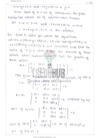
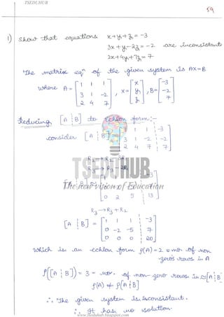
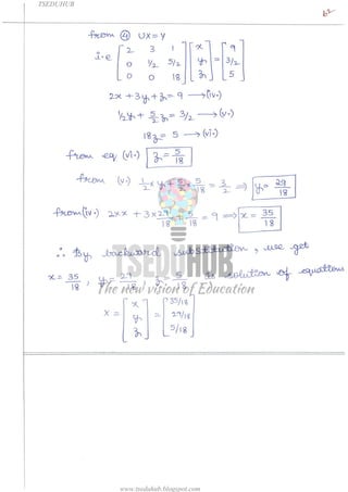
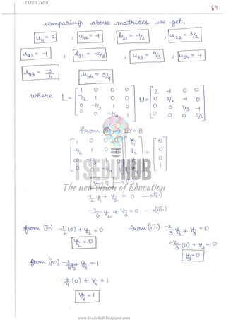
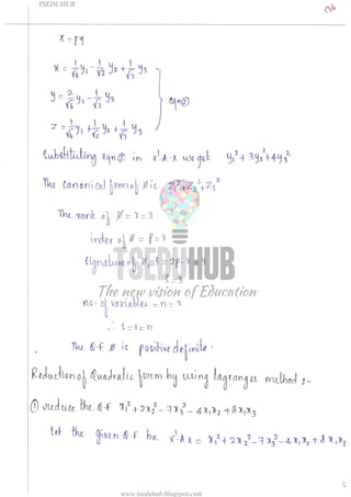
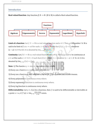
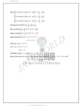
SlideShare a Scribd company logo
TSEDUHUB
www.tseduhub.blogspot.com
TSEDUHUB
www.tseduhub.blogspot.com
TSEDUHUB
www.tseduhub.blogspot.com
TSEDUHUB
www.tseduhub.blogspot.com
TSEDUHUB
www.tseduhub.blogspot.com
TSEDUHUB
www.tseduhub.blogspot.com
TSEDUHUB
www.tseduhub.blogspot.com
TSEDUHUB
www.tseduhub.blogspot.com
TSEDUHUB
www.tseduhub.blogspot.com
TSEDUHUB
www.tseduhub.blogspot.com
TSEDUHUB
www.tseduhub.blogspot.com
TSEDUHUB
www.tseduhub.blogspot.com
TSEDUHUB
www.tseduhub.blogspot.com
TSEDUHUB
www.tseduhub.blogspot.com
TSEDUHUB
www.tseduhub.blogspot.com
TSEDUHUB
www.tseduhub.blogspot.com
TSEDUHUB
www.tseduhub.blogspot.com
TSEDUHUB
www.tseduhub.blogspot.com
TSEDUHUB
www.tseduhub.blogspot.com
TSEDUHUB
www.tseduhub.blogspot.com
TSEDUHUB
www.tseduhub.blogspot.com
TSEDUHUB
www.tseduhub.blogspot.com
TSEDUHUB
www.tseduhub.blogspot.com
TSEDUHUB
www.tseduhub.blogspot.com
TSEDUHUB
www.tseduhub.blogspot.com
TSEDUHUB
www.tseduhub.blogspot.com
TSEDUHUB
www.tseduhub.blogspot.com
TSEDUHUB
www.tseduhub.blogspot.com
TSEDUHUB
www.tseduhub.blogspot.com
TSEDUHUB
www.tseduhub.blogspot.com
TSEDUHUB
www.tseduhub.blogspot.com
TSEDUHUB
www.tseduhub.blogspot.com
TSEDUHUB
www.tseduhub.blogspot.com
TSEDUHUB
www.tseduhub.blogspot.com
TSEDUHUB
www.tseduhub.blogspot.com
TSEDUHUB
www.tseduhub.blogspot.com
TSEDUHUB
www.tseduhub.blogspot.com
TSEDUHUB
www.tseduhub.blogspot.com
TSEDUHUB
www.tseduhub.blogspot.com
TSEDUHUB
www.tseduhub.blogspot.com
TSEDUHUB
www.tseduhub.blogspot.com
TSEDUHUB
www.tseduhub.blogspot.com
TSEDUHUB
www.tseduhub.blogspot.com
TSEDUHUB
www.tseduhub.blogspot.com
TSEDUHUB
www.tseduhub.blogspot.com
TSEDUHUB
www.tseduhub.blogspot.com
TSEDUHUB
www.tseduhub.blogspot.com
TSEDUHUB
www.tseduhub.blogspot.com
TSEDUHUB
www.tseduhub.blogspot.com
TSEDUHUB
www.tseduhub.blogspot.com
TSEDUHUB
www.tseduhub.blogspot.com
TSEDUHUB
www.tseduhub.blogspot.com
TSEDUHUB
www.tseduhub.blogspot.com
TSEDUHUB
www.tseduhub.blogspot.com
TSEDUHUB
www.tseduhub.blogspot.com
TSEDUHUB
www.tseduhub.blogspot.com
TSEDUHUB
www.tseduhub.blogspot.com
TSEDUHUB
www.tseduhub.blogspot.com
TSEDUHUB
www.tseduhub.blogspot.com
TSEDUHUB
www.tseduhub.blogspot.com
TSEDUHUB
www.tseduhub.blogspot.com
TSEDUHUB
www.tseduhub.blogspot.com
TSEDUHUB
www.tseduhub.blogspot.com
TSEDUHUB
www.tseduhub.blogspot.com
TSEDUHUB
www.tseduhub.blogspot.com
TSEDUHUB
www.tseduhub.blogspot.com
TSEDUHUB
www.tseduhub.blogspot.com
TSEDUHUB
www.tseduhub.blogspot.com
TSEDUHUB
www.tseduhub.blogspot.com
TSEDUHUB
www.tseduhub.blogspot.com
TSEDUHUB
www.tseduhub.blogspot.com
TSEDUHUB
www.tseduhub.blogspot.com
TSEDUHUB
www.tseduhub.blogspot.com
TSEDUHUB
www.tseduhub.blogspot.com
TSEDUHUB
www.tseduhub.blogspot.com
TSEDUHUB
www.tseduhub.blogspot.com
TSEDUHUB
www.tseduhub.blogspot.com
TSEDUHUB
www.tseduhub.blogspot.com
TSEDUHUB
www.tseduhub.blogspot.com
TSEDUHUB
www.tseduhub.blogspot.com
TSEDUHUB
www.tseduhub.blogspot.com
TSEDUHUB
www.tseduhub.blogspot.com
TSEDUHUB
www.tseduhub.blogspot.com
TSEDUHUB
www.tseduhub.blogspot.com
TSEDUHUB
www.tseduhub.blogspot.com
TSEDUHUB
www.tseduhub.blogspot.com
TSEDUHUB
www.tseduhub.blogspot.com
TSEDUHUB
www.tseduhub.blogspot.com
TSEDUHUB
www.tseduhub.blogspot.com
TSEDUHUB
www.tseduhub.blogspot.com
TSEDUHUB
www.tseduhub.blogspot.com
TSEDUHUB
www.tseduhub.blogspot.com
TSEDUHUB
www.tseduhub.blogspot.com
TSEDUHUB
www.tseduhub.blogspot.com
TSEDUHUB
www.tseduhub.blogspot.com
TSEDUHUB
www.tseduhub.blogspot.com
TSEDUHUB
www.tseduhub.blogspot.com
TSEDUHUB
www.tseduhub.blogspot.com
TSEDUHUB
www.tseduhub.blogspot.com
TSEDUHUB
www.tseduhub.blogspot.com
TSEDUHUB
www.tseduhub.blogspot.com
TSEDUHUB
www.tseduhub.blogspot.com
TSEDUHUB
www.tseduhub.blogspot.com
TSEDUHUB
www.tseduhub.blogspot.com
TSEDUHUB
www.tseduhub.blogspot.com
TSEDUHUB
www.tseduhub.blogspot.com
TSEDUHUB
www.tseduhub.blogspot.com
TSEDUHUB
www.tseduhub.blogspot.com
TSEDUHUB
www.tseduhub.blogspot.com
TSEDUHUB
www.tseduhub.blogspot.com
TSEDUHUB
www.tseduhub.blogspot.com
TSEDUHUB
www.tseduhub.blogspot.com
TSEDUHUB
www.tseduhub.blogspot.com
TSEDUHUB
www.tseduhub.blogspot.com
TSEDUHUB
www.tseduhub.blogspot.com
TSEDUHUB
www.tseduhub.blogspot.com
TSEDUHUB
www.tseduhub.blogspot.com
TSEDUHUB
www.tseduhub.blogspot.com
TSEDUHUB
www.tseduhub.blogspot.com
TSEDUHUB
www.tseduhub.blogspot.com
TSEDUHUB
www.tseduhub.blogspot.com
TSEDUHUB
www.tseduhub.blogspot.com
TSEDUHUB
www.tseduhub.blogspot.com
TSEDUHUB
www.tseduhub.blogspot.com
TSEDUHUB
www.tseduhub.blogspot.com
TSEDUHUB
www.tseduhub.blogspot.com
TSEDUHUB
www.tseduhub.blogspot.com
TSEDUHUB
www.tseduhub.blogspot.com
TSEDUHUB
www.tseduhub.blogspot.com
TSEDUHUB
www.tseduhub.blogspot.com
JNTUWORLD
MATHEMATICS-I
MEAN VALUE THEOREMS
FUNCTIONS OF SINGLE
&
SEVERAL VARIABLES
I YEAR B.TECH
By
Y. Prabhaker Reddy
Asst. Professor of Mathematics
Guru Nanak Engineering College
Ibrahimpatnam, Hyderabad.
TSEDUHUB
www.tseduhub.blogspot.com
JNTUWORLD
SYLLABUS OF MATHEMATICS-I (AS PER JNTU HYD)
Name of the Unit Name of the Topic
Unit-I
Sequences and Series
Basic definition of sequences and series
Convergence and divergence.
Ratio test
Comparison test
Integral test
Cauchy’s root test
Raabe’s test
Absolute and conditional convergence
Unit-II
Functions of single variable
Rolle’s theorem
Lagrange’s Mean value theorem
Cauchy’s Mean value theorem
Generalized mean value theorems
Functions of several variables
Functional dependence, Jacobian
Maxima and minima of function of two variables
Unit-III
Application of single variables
Radius , centre and Circle of curvature
Evolutes and Envelopes
Curve Tracing-Cartesian Co-ordinates
Curve Tracing-Polar Co-ordinates
Curve Tracing-Parametric Curves
Unit-IV
Integration and its
applications
Riemann Sum
Integral representation for lengths
Integral representation for Areas
Integral representation for Volumes
Surface areas in Cartesian and Polar co-ordinates
Multiple integrals-double and triple
Change of order of integration
Change of variable
Unit-V
Differential equations of first
order and their applications
Overview of differential equations
Exact and non exact differential equations
Linear differential equations
Bernoulli D.E
Newton’s Law of cooling
Law of Natural growth and decay
Orthogonal trajectories and applications
Unit-VI
Higher order Linear D.E and
their applications
Linear D.E of second and higher order with constant coefficients
R.H.S term of the form exp(ax)
R.H.S term of the form sin ax and cos ax
R.H.S term of the form exp(ax) v(x)
Method of variation of parameters
Applications on bending of beams, Electrical circuits and simple harmonic motion
Unit-VII
Laplace Transformations
LT of standard functions
Inverse LT –first shifting property
Transformations of derivatives and integrals
Unit step function, Second shifting theorem
Convolution theorem-periodic function
Differentiation and integration of transforms
Application of laplace transforms to ODE
Unit-VIII
Vector Calculus
Gradient, Divergence, curl
Laplacian and second order operators
Line, surface , volume integrals
Green’s Theorem and applications
Gauss Divergence Theorem and applications
Stoke’s Theorem and applications
TSEDUHUB
www.tseduhub.blogspot.com
JNTUWORLD
CONTENTS
UNIT-2
Functions of Single & Several Variables
 Rolle’s Theorem without Proof
 Lagrange’s Mean Value Theorem without Proof
 Cauchy’s Mean Value Theorem without Proof
 Generalized Mean Value Theorem (without Proof)
 Functions of Several Variables-Functional dependence
 Jacobian
 Maxima and Minima of functions of two variables
TSEDUHUB
www.tseduhub.blogspot.com
JNTUWORLD
Introduction
Real valued function: Any function is called a Real valued function.
Limit of a function: Let is a real valued function and . Then, a real number is
said to be limit of at if for each whenever
. It is denoted by .
Continuity: Let is a real valued function and . Then, is said to be continuous at
if for each whenever . It is
denoted by .
Note: 1) The function is continuous every where
2) Every function is continuous every where.
3) Every function is not continuous, but in the function is continuous.
4) Every polynomial is continuous every where.
5) Every exponential function is continuous every where.
6) Every log function is continuous every where.
Differentiability: Let be a function, then is said to be differentiable or derivable at
a point , if exists.
Functions
Algebraic Trignonometric Inverse Exponential Logarithmic Hyperbolic
TSEDUHUB
www.tseduhub.blogspot.com
JNTUWORLD
MEAN VALUE THEOREMS
Let be a given function.
ROLLE’S THEOREM
Let such that
(i) is continuous in
(ii) is differentiable (or) derivable in
(iii)
then atleast one point in such that
Geometrical )nterpretation of Rolle’s Theorem:
From the diagram, it can be observed that
(i) there is no gap for the curve from . Therefore, the function is
continuous
(ii) There exists unique tangent for every intermediate point between and
(ii) Also the ordinates of and are same, then by Rolle’s theorem, there exists atleast one point
in between and such that tangent at is parallel to axis.
LAGRANGE’S MEAN VALUE THEOREM
Let such that
(i) is continuous in
(ii) is differentiable (or) derivable in
then atleast one point such that
TSEDUHUB
www.tseduhub.blogspot.com
JNTUWORLD
Geometrical )nterpretation of Rolle’s Theorem:
From the diagram, it can be observed that
(i) there is no gap for the curve from . Therefore, the function is
continuous
(ii) There exists unique tangent for every intermediate point between and
Then by Lagrange’s mean value theorem, there exists atleast one point in between and
such that tangent at is parallel to a straight line joining the points and
CAUCHY’S MEAN VALUE THEOREM
Let are such that
(i) are continuous in
(ii) are differentiable (or) derivable in
(iii)
then atleast one point such that
Generalised Mean Value Theorems
Taylor’s Theorem: If such that
(i) are continuous on
(ii) are derivable or differentiable on
(iii) , then such that
where, is called as Schlomilch – Roche’s form of remainder and is given by
TSEDUHUB
www.tseduhub.blogspot.com
JNTUWORLD
 Lagrange’s form of Remainder:
Substituting in we get Lagrange’s form of Remainder
i.e.
 Cauchy’s form of Remainder:
Substituting in we get Cauchy’s form of Remainder
i.e.
Maclaurin’s Theorem: If such that
(i) are continuous on
(ii) are derivable or differentiable on
(iii) , then such that
where, is called as Schlomilch – Roche’s form of remainder and is given by
 Lagrange’s form of Remainder:
Substituting in we get Lagrange’s form of Remainder
i.e.
 Cauchy’s form of Remainder:
Substituting in we get Cauchy’s form of Remainder
i.e.
TSEDUHUB
www.tseduhub.blogspot.com
JNTUWORLD
Jacobian
Let are two functions , then the Jacobian of w.r.t is
denoted by and is defined as
Properties:

 If are functions of and are functions of then
Functional Dependence:
Two functions are said to be functional dependent on one another if the Jacobian of
is zero.
If they are functionally dependent on one another, then it is possible to find the relation between
these two functions.
MAXIMA AND MINIMA
Maxima and Minima for the function of one Variable:
Let us consider a function
To find the Maxima and Minima, the following procedure must be followed:
Step 1: First find the first derivative and equate to zero. i.e.
Step 2: Since is a polynomial is a polynomial equation. By solving this
equation we get roots.
Step 3: Find second derivative i.e.
Step 4: Now substitute the obtained roots in
Step 5: Depending on the Nature of at that point we will solve further. The following cases will
be there.
TSEDUHUB
www.tseduhub.blogspot.com
JNTUWORLD
Case (i): If at a point say , then has maximum at and the maximum
value is given by
Case (ii): If at a point say , then has minimum at and the minimum
value is given by
Case (iii): If at a point say , then has neither minimum nor maximum. i.e.
stationary.
Maxima and Minima for the function of Two Variable
Let us consider a function
To find the Maxima and Minima for the given function, the following procedure must be followed:
Step 1: First find the first derivatives and equate to zero. i.e.
(Here, since we have two variables, we go for partial derivatives, but not ordinary
derivatives)
Step 2: By solving , we get the different values of and .
Write these values as set of ordered pairs. i.e.
Step 3: Now, find second order partial derivatives.
i.e.,
Step 4: Let us consider ,
Step 5: Now, we have to see for what values of , the given function is maximum/minimum/
does not have extreme values/ fails to have maximum or minimum.
 If at a point, say , then has maximum at this point and the
maximum value will be obtained by substituting in the given function.
 If at a point, say , then has minimum at this point and the
minimum value will be obtained by substituting in the given function.
 If at a point, say , then has neither maximum nor minimum and
such points are called as saddle points.
 If at a point, say , then fails to have maximum or minimum and case
needs further investigation to decide maxima/minima. i.e. No conclusion
TSEDUHUB
www.tseduhub.blogspot.com
JNTUWORLD
Problem
1) Examine the function for extreme values
Sol: Given
The first order partial derivatives of are given by
and
Now, equating first order partial derivatives to zero, we get
Solving we get
Substituting in
Substituting in
All possible set of values are
Now, the second order partial derivatives are given by
Now,
At a point &
has maximum at and the maximum value will be obtained by substituting in the
function
i.e. is the maximum value.
TSEDUHUB
www.tseduhub.blogspot.com
JNTUWORLD
Also, at a point &
has minimum at and the minimum value is .
Also, at a point
has neither minimum nor maximum at this point.
Again, at a point
has neither minimum nor maximum at this point.
Lagrange’s Method of Undetermined Multipliers
This method is useful to find the extreme values (i.e., maximum and minimum) for the given
function, whenever some condition is given involving the variables.
To find the Maxima and Minima for the given function using Lagrange’s Method , the following
procedure must be followed:
Step 1: Let us consider given function to be subject to the condition
Step 2: Let us define a Lagrangean function , where is called the Lagrange
multiplier.
Step 3: Find first order partial derivatives and equate to zero
i.e.
Let the given condition be
Step 4: Solve , eliminate to get the values of
Step 5: The values so obtained will give the stationary point of
Step 6: The minimum/maximum value will be obtained by substituting the values of in the
given function.
Problem
1) Find the minimum value of subject to the condition
Sol: Let us consider given function to be and
Let us define Lagrangean function , where is called the Lagrange multiplier.
TSEDUHUB
www.tseduhub.blogspot.com
JNTUWORLD
Now,
Solving
Now, consider
Again, consider
Again solving
Given
Similarly, we get
Hence, the minimum value of the function is given by
TSEDUHUB
www.tseduhub.blogspot.com
JNTUWORLD
MATHEMATICS-I
Curvature, Evolutes & Envelopes
Curve Tracing
I YEAR B.Tech
By
Y. Prabhaker Reddy
Asst. Professor of Mathematics
Guru Nanak Engineering College
Ibrahimpatnam, Hyderabad.
TSEDUHUB
www.tseduhub.blogspot.com
JNTUWORLD
UNIT-III
CURVATURE
The shape of a plane Curve is characterized by the degree of Bentness or Curvedness.
RADIUS OF CURVATURE
The reciprocal of the curvature of a curve is called the radius of curvature of curve.
FORMULAE FOR THE EVALUATION OF RADIUS OF CURVATURE
In this we have three types of problems
Problems to find Radius of Curvature in Cartesian Co-ordinates
Problems to find Radius of Curvature in Polar Co-ordinates
Problems to find Radius of Curvature in Parametric Form.
In Cartesian Co-ordinates
Let us consider be the given curve, then radius of curvature is given by
If the given equation of the curve is given as , then the radius of curvature is given
by
TSEDUHUB
www.tseduhub.blogspot.com
JNTUWORLD
In Parametric Form
(i.e. in terms of other variable and in terms of other variable say
)
If the equation of the curve is given in parametric form then
In Polar co-ordinates
If the equation of the curve is given in polar form i.e. then
where, and .
Radius of Curvature at origin Newton s Theorem
Suppose a curve is passing through the origin and -axis or -axis is tangent to the curve at
the origin. Then the following results will be useful to find at
If -axis is tangent at , then
Note: If the given curve passes through and neither -axis nor -axis is
tangent to the curve, then
Using Maclaurin s series expansion of , we get
TSEDUHUB
www.tseduhub.blogspot.com
JNTUWORLD
then,
By this we can calculate at using the formula for finding Radius of Curvature in
Cartesian Co-ordinates.
Problems on Radius of Curvature
1) Find the radius of curvature at the point of the curve .
Sol: Clearly, the given equation of curve belongs to Cartesian coordinates.
We know that, the radius of curvature at any point on the curve is given by
Now, consider
Differentiate w.r.t , we get
Here,
Again, differentiating , w.r.t , we get
TSEDUHUB
www.tseduhub.blogspot.com
JNTUWORLD
Now, the Radius of curvature at is given by
numerically… since radius cannot be negative
2) If be the radius of curvature at the extremities of an chord of the cardioid
which passes through the pole, show that
Sol: Let us consider the equation of the cardioids to be
Let us consider to be the extremities of the chord,
whose coordinates are given by and
Let be the radius of curvature at the point and
respectively.
Let us find :
We know that the radius of curvature for the curve is given by
Now, consider
and
Hence,
TSEDUHUB
www.tseduhub.blogspot.com
JNTUWORLD
Similarly,
Now, consider L.H.S:
i.e.
.
3) Show that the radius of curvature at each point of the curve
,
is inversely proportional to the length of the normal intercepted between the
point on the curve and the axis.
Sol: Clearly, the equation of the curve is in parametric form
Let us change the problem of solving radius of curvature in parametric form to problem of
solving radius of curvature in Cartesian form.
Here, given
TSEDUHUB
www.tseduhub.blogspot.com
JNTUWORLD
Similarly,
Now,
Again,
Hence, the radius of curvature for the equation of the curve at any point is given
by
TSEDUHUB
www.tseduhub.blogspot.com
JNTUWORLD
Also, we know that the length of the normal is given by
Hence, from we can say that, the radius of curvature at each point of the curve
is inversely proportional to the length of the normal
intercepted between the point on the curve and the axis.
Hence the result.
CENTRE OF CURVATURE
Definition : The Centre of Curvature at a point P of a curvature is the point C which lies
on the Positive direction of the normal at P and is at a distance (in magnitude) from it.
CIRCLE OF CURVATURE
Definition: The circle of curvature at a point P of a curve is the circle whose centre is at
the centre of Curvature C and whose radius is in magnitude
TSEDUHUB
www.tseduhub.blogspot.com
JNTUWORLD
Problems on Centre of Curvature and circle of curvature
1) Find the centre of curvature at the point of the curve . Find
also the equation of the circle of curvature at that point.
Sol: We know that, if are the coordinates of the centre of curvature at any point
on the curve , then
Now, given
Differentiate w.r.t , we get
Now,
Again, Differentiate (1) w.r.t , we get
Hence, the coordinates of the centre of curvature are
TSEDUHUB
www.tseduhub.blogspot.com
JNTUWORLD
Hence,
Now, radius of curvature at the point is given by
Hence, the equation of circle of curvature at the given point is given by
EVOLUTE
Corresponding to each point on a curve we can find the curvature of the curve at that point.
Drawing the normal at these points, we can find Centre of Curvature corresponding to each
of these points. Since the curvature varies from point to point, centres of curvature also
differ. The totality of all such centres of curvature of a given curve will define another curve
and this curve is called the evolute of the curve.
The Locus of centres of curvature of a given curve is called the evolute of that curve.
The locus of the centre of curvature of a variable point on a curve is called the evolute
of the curve. The curve itself is called involute of the evolute.
TSEDUHUB
www.tseduhub.blogspot.com
JNTUWORLD
Here, for different points on the curve, we get different centre of curvatures. The locus of all
these centres of curvature is called as Evolute.
The external curve which satisfies all these centres of curvature is called as Evolute. Here
Evolute is nothing but an curve equation.
To find Evolute, the following models exist.
1) If an equation of the curve is given and If we are asked to show / prove L.H.S=R.H.S,
Then do as follows.
First find Centre of Curvature , where
And then consider L.H.S: In that directly substitute in place of and in place of
. Similarly for R.H.S. and then show that L.H.S=R.H.S
2) If a curve is given and if we are asked to find the evolute of the given curve, then do
as follows:
First find Centre of curvature and then re-write as
in terms of and in terms of . and then substitute in the given curve, which
gives us the required evolute.
3) If a curve is given, which is in parametric form, then first find Centre of curvature,
which will be in terms of parameter. then using these values of and eliminate
the parameter, which gives us evolute.
TSEDUHUB
www.tseduhub.blogspot.com
JNTUWORLD
Problem
1) Find the coordinates of centre of curvature at any point of the parabola
and also show its evolute is given by
Sol: Given curve is
We know that, if are the coordinates of the centre of curvature at any point
on the curve , then
Now,
Also,
Consider,
TSEDUHUB
www.tseduhub.blogspot.com
JNTUWORLD
Consider,
Now, required to prove is
L.H.S
R.H.S
Hence,
Hence the Result.
ENVELOPE
A curve which touches each member of a given family of curves is called envelope of that
family.
Procedure to find envelope for the given family of curves:
Case 1: Envelope of one parameter
Let us consider to be the given family of curves.
Step 1: Differentiate w.r.t to the parameter partially, and find the value of the parameter
TSEDUHUB
www.tseduhub.blogspot.com
JNTUWORLD
Step 2: By Substituting the value of parameter in the given family of curves, we get
required envelope.
Special Case: If the given equation of curve is quadratic in terms of parameter, then
envelope is given by
Case 2: Envelope of two parameter
Let us consider to be the given family of curves, and a relation connecting these
two parameters
Step 1: Obtain one parameter in terms of other parameter from the given relation
Step 2: Substitute in the given equation of curve, so that the problem of two parameter
converts to problem of one parameter.
Step 3: Use one parameter technique to obtain envelope for the given family of curve
Problem
1) Find the envelope of the family of straight line is the
parameter.
Sol: Given equation of family of curves is
Step 1: Differentiate partially w.r.t the parameter
Step 2: Substitute the value of in the given family of curves
TSEDUHUB
www.tseduhub.blogspot.com
JNTUWORLD
The envelope of the given family of straight lines is an ellipse.
2) Find the envelope of family of straight line , where are two
parameters which are connected by the relation .
Sol: Given equation of family of straight lines is
Also given,
Substituting in , we get
Step 1: Differentiate w.r.t partially, we get
TSEDUHUB
www.tseduhub.blogspot.com
JNTUWORLD
Now, substitute the value of in
Step 2: Substitute the values of in the given family of curves , we get
is the required envelope
TSEDUHUB
www.tseduhub.blogspot.com
JNTUWORLD
CURVE TRACING
Drawing a rough sketch of the curve is called as Curve Tracing.
Aim: To find the appropriate shape of a curve for the given equation.
METHOD OF TRACING CURVES
Cartesian Co-ordinates: In order to obtain general shape of the curve from the given
equations, we have to examine the following properties.
1) SYMMETRY
a) If the equation contains even powers of only, the curve is symmetrical about
Example:
b) If the equation contains even powers of only, the curve is symmetrical about
Example:
c) If all the powers of and in the given equation are even, the curve is symmetrical
about the both the axes. i.e. about the origin.
Example:
d) If the equations of the curve is not changed by interchanging and , then the curve
is symmetrical about the line .
Example:
e) If the equation of a curve remains unchanged when both and are interchanged by
– and – respectively, then the curve is symmetrical in opposite-quadrants.
Examples:
TSEDUHUB
www.tseduhub.blogspot.com
JNTUWORLD
2) ORIGIN
If the equation of a curve is satisfied by then the curve passes through
the origin.
Example:
3) INTERSECTION WITH CO-ORDINATE AXIS
Put in the given equation to get points of intersection with
4) REGION
If possible write the given equation in the form of Give values of to make
imaginary. Let be imaginary for the values of lying between and .
Then, no part of the curve lies between and . Similarly, the curve does
not lies between those values of for which is imaginary.
5) TANGENTS
a) If the curve passes through the origin, the tangents at the origin are given by
equating the lowest degree terms to zero.
Example: For the curve , the tangents are given by equating the
lowest degree terms to zero. i.e. are tangents at origin.
b) If the curve is not passing through the origin, the tangents at any point are given
by finding at that point and this indicates the direction of the tangent at that
point.
Note: If there are two tangents at the origin, the origin is a double point.
A) If the two tangents are real and coincident, the origin is a cusp.
B) If the two tangents are real and different, the origin is a node.
TSEDUHUB
www.tseduhub.blogspot.com
JNTUWORLD
C) If the two tangents are Imaginary, the origin is a conjugate point or Isolated
point.
6) EXTENSION OF THE CURVE TO INFINITY
Give values to for which the value of is Infinity and also give values to for which
is Infinity. These values indicate the direction in which the curve extends to
Infinity.
7) ASYMPTOTES
An Asymptote is a straight line which cuts a curve in two points, at an infinite
distance from the origin and yet is not itself wholly at Infinity.
To find Asymptotes
a) Asymptotes parallel to axis
Asymptotes parallel to -axis are obtained by equating the coefficient
of the highest power of to zero.
Asymptotes parallel to -axis are obtained by equating the coefficient
of the highest power of to zero.
b) Oblique Asymptotes: ( Asymptotes which are not parallel to axis)
Let be an asymptote. Put in the given equation of the curve.
Equate the coefficients of highest powers of to zero and solve for and .
TSEDUHUB
www.tseduhub.blogspot.com
JNTUWORLD
Problems on Curve Tracing - Cartesian Coordinates
1) Trace the curve
Sol: In order to trace a curve, we need to check the following properties
 Symmetry
 Origin
 Intersection with coordinate axis
 Region
 Tangents
 Intersection of curve to
 Asymptotes
Let us consider given equation of curve to be
Symmetry: If we interchange and , the equation of
curve is not changing.
Hence, the curve is symmetric about the line
Origin: If we substitute and , the equation of
curve is satisfied.
Hence, we can say that the curve passes through the
origin.
Intersection with coordinate axis:
Put
The curve meets the axis only at the Origin
Again
The curve meets the axis only at the Origin
Region: Consider
is positive is also positive
The curve lies in 1st Quadrant
is negative is positive
The curve lies in 2nd Quadrant
is negative & is negative
TSEDUHUB
www.tseduhub.blogspot.com
JNTUWORLD
Then the equation of curve is not satisfied
The curve does not lie in 3rd Quadrant
is positive is negative
The curve lies in 4th Quadrant
Tangents: The given equation of curve passes through
Origin.
Hence, the tangents at origin are given by equating lowest degree terms to zero.
i.e.,
There exists two tangents namely,
Here, the two tangents at origin are real and distinct. Hence, we get a node
Now, let us check, at what points the curve meets the line
Hence, the curve meets at
Extension of the curve to Infinity:
As
The curve extends to infinity in the second quadrant.
Also, as
The curve extends to infinity in the fourth quadrant.
Asymptotes:
TSEDUHUB
www.tseduhub.blogspot.com
JNTUWORLD
Asymptotes parallel to axis:
No Asymptote is parallel to
Asymptotes not parallel to axis (Oblique Asymptotes)
Let us consider to be the required asymptote.
Now, substitute in the given equation of the curve and solving for and , we get
Hence, the required asymptote is
Hence the shape of the curve is as follows
TSEDUHUB
www.tseduhub.blogspot.com
JNTUWORLD
PROCEDURE FOR TRACING CURVES IN POLAR CO-ORDINATES
1) SYMMETRY
i) If the equation does not alter by changing to – , the curve is symmetrical about the
initial line or -axis.
Example:
ii) If the equation does not alter by changing to – , the curve is symmetrical about the
pole.
Example:
iii) If the equation of the curve remains unaltered when is changed to or by changing
to – to – , the curve is symmetric about the line or -axis.
Example:
iv) If the equation of the curve remains unaltered when is changed to , then the curve
is symmetrical about the line
Example:
v) If the equation of the curve does not alter by changing to then the curve is
symmetrical about the line
Example: .
2) Discussion for and
Give certain values to and find the corresponding values of and then plot the points.
Sometimes it is inconvenient to find the corresponding values of for certain values of . In
such cases, a particular region for may be considered and find out whether increases or
decreases in that region.
For example: It is inconvenient to find the value of for but it is equal to know
whether increases or decreases in the region from to in which value is also
included.
3) Region
No part of the curve exists for those values of which make corresponding value of
imaginary.
TSEDUHUB
www.tseduhub.blogspot.com
JNTUWORLD
4) Tangents
Find , where is the angle between the radius vector and the tangent at
. It will indicate the direction of the tangents at any point .
5) Asymptotes
Find the value of which makes infinity. The curve has an asymptote in that direction.
TSEDUHUB
www.tseduhub.blogspot.com
JNTUWORLD
By
Y. Prabhaker Reddy
Asst. Professor of Mathematics
Guru Nanak Engineering College
Ibrahimpatnam, Hyderabad.
MATHEMATICS-I
APPLICATIONS OF INTEGRATION
I YEAR B.Tech
TSEDUHUB
www.tseduhub.blogspot.com
JNTUWORLD
UNIT-4
APPLICATIONS OF INTEGRATION
Riemann Integrals:
Let us consider an interval with
If , then a finite set is
called as a partition of and it is denoted by .
The sub intervals are called segments (or)
sub intervals.
The sub interval in this process is and its length is given by
Note: For every interval , it is possible to define infinitely many partitions.
Norm (or) Mesh of the partition: The maximum of the lengths of the sub intervals
w.r.t the partition is called as Norm of the partition (or) Mesh of the partition and
it is denoted by
Refinement: If and are two partitions of and if , then is called as
Refinement of .
Lower and Upper Reimann Sum’s
Let is bounded and be a partition on ,
then sub interval is given by and its length is given by
If is bounded on , then is bounded on
let and be Infimum and supremum of on , then
 The sum is called as lower Reimann sum and it is denoted by
 The sum is called as upper Reimann sum and it is denoted by
Note: Always,
TSEDUHUB
www.tseduhub.blogspot.com
JNTUWORLD
Problem
1) If and be a partition of then compute
Sol: Given defined on and be a partition of
Here, let
And,
Let and be Infimum and supremum of on , then
Hence,
Also,
Lower Reimann Integral: Let be a bounded function and is a partition
of , then supremum of is called as Lower Reimann integral on
and it is denoted by
Upper Reimann Integral: Let be a bounded function and is a partition
of , then Infimum of is called as Upper Reimann integral on
and it is denoted by
Riemann Integral
If be a bounded function and is a partition of and if
, then is said to be Riemann integrable on and it is denoted by
TSEDUHUB
www.tseduhub.blogspot.com
JNTUWORLD
Rectification: The process of finding the length of the arc of the curve is called as
Rectification
Length of the arc of the curve
Equation of the curve Arc Length
Cartesian Form
(i) and and
(ii) and and
Parametric Form
and and
Polar Form
(i) and and
(ii) and and
Problems on length of the arc of the curve
1) Find the length of the arc of the curve from to .
Solution: We know that, the equation of the length of the arc of the curve
between and is given by
Given
TSEDUHUB
www.tseduhub.blogspot.com
JNTUWORLD
The required length of the arc of the curve is given by
2) Find the perimeter of the loop of the curve
Solution: We know that, the equation of the length of the arc of the curve
between and is given by
Given
TSEDUHUB
www.tseduhub.blogspot.com
JNTUWORLD
Now,
Here the curve is symmetrical about the . Hence the length of the arc will be
double that of the arc of the loop about the .
The required length of the loop is =
TSEDUHUB
www.tseduhub.blogspot.com
JNTUWORLD
3) Find the perimeter of the cardioids .
Solution: We know that the length of the arc of the curve and is
given by
Given
The cardioids is symmetrical about the initial line and passes through the pole.
Hence the length of the arc will be double that of the arc of the loop about the .
The required length of the loop is =
TSEDUHUB
www.tseduhub.blogspot.com
JNTUWORLD
4)
TSEDUHUB
www.tseduhub.blogspot.com
JNTUWORLD
Volume of solid of Revolution
Region (R) Axis
Volume of the solid
generated
Cartesian form
(i) , the and the lines
and
(ii) , the and the lines
and
(iii)
(iv)
Parametric form
(i)
(ii)
Polar form
(i)
The initial
line
(ii)
The line
(iii)
The line
Problems on Volume of solid of Revolution
1) Find the volume of the solid that result when the region enclosed by the curve
is revolved about the .
Sol: We know that the volume of the solid generated by the revolution of the area
bounded by the curve , the and the lines is given by
Now, given curve
Required volume is given by
TSEDUHUB
www.tseduhub.blogspot.com
JNTUWORLD
2) Find the volume of the solid generated by the revolution of the cardioids
about the initial line.
Sol: We know that the volume of the solid generated by the revolution of the area
bounded by the curve , the initial line and is given by
Here, the given cardioids is symmetrical about the initial line. The upper half of the
curve formed when varies from to .
TSEDUHUB
www.tseduhub.blogspot.com
JNTUWORLD
Surface area of solid of Revolution
Equation of the curve Arc Length
Cartesian Form
(i) and and ,
(ii) and and ,
Parametric Form
(i) and and
(ii) and and
Polar Form
(i) and and
(ii) and and
Problem
1) Find the surface area generated by the revolution of an arc of the catenary
about the
Sol: We know that the surface area of the solid generated by the revolution of an arc
about the , is given by
TSEDUHUB
www.tseduhub.blogspot.com
JNTUWORLD
2) Find the surface area of the solid formed by revolving the cardioid
about the initial line.
Sol: We know that the surface area of the solid formed by revolving the cardioid
, the initial line and is given by
Given
The cardioid is symmetrical about the initial line and passes through the pole.
Hence, required surface area is given by
TSEDUHUB
www.tseduhub.blogspot.com
JNTUWORLD
Let
Lower Limit:
Upper Limit:
Surface area –
Change of variables in Double Integral
Problem:
Solution: Clearly, given coordinates are in Cartesian.
TSEDUHUB
www.tseduhub.blogspot.com
JNTUWORLD
2)
Solution:
TSEDUHUB
www.tseduhub.blogspot.com
JNTUWORLD
TSEDUHUB
www.tseduhub.blogspot.com
JNTUWORLD
Change of Order of Integration
Problem 1:
TSEDUHUB
www.tseduhub.blogspot.com
JNTUWORLD
2)
3)
TSEDUHUB
www.tseduhub.blogspot.com
JNTUWORLD
4)
TSEDUHUB
www.tseduhub.blogspot.com
JNTUWORLD
TSEDUHUB
www.tseduhub.blogspot.com
JNTUWORLD
By
Y. Prabhaker Reddy
Asst. Professor of Mathematics
Guru Nanak Engineering College
Ibrahimpatnam, Hyderabad.
MATHEMATICS-I
DIFFERENTIAL EQUATIONS-I
I YEAR B.TECH
TSEDUHUB
www.tseduhub.blogspot.com
JNTUWORLD
SYLLABUS OF MATHEMATICS-I (AS PER JNTU HYD)
Name of the Unit Name of the Topic
Unit-I
Sequences and Series
1.1 Basic definition of sequences and series
1.2 Convergence and divergence.
1.3 Ratio test
1.4 Comparison test
1.5 Integral test
1.6 Cauchy s root test
1.7 Raabe s test
1.8 Absolute and conditional convergence
Unit-II
Functions of single variable
. Rolle s theorem
. Lagrange s Mean value theorem
. Cauchy s Mean value theorem
2.4 Generalized mean value theorems
2.5 Functions of several variables
2.6 Functional dependence, Jacobian
2.7 Maxima and minima of function of two variables
Unit-III
Application of single variables
3.1 Radius , centre and Circle of curvature
3.2 Evolutes and Envelopes
3.3 Curve Tracing-Cartesian Co-ordinates
3.4 Curve Tracing-Polar Co-ordinates
3.5 Curve Tracing-Parametric Curves
Unit-IV
Integration and its
applications
4.1 Riemann Sum
4.3 Integral representation for lengths
4.4 Integral representation for Areas
4.5 Integral representation for Volumes
4.6 Surface areas in Cartesian and Polar co-ordinates
4.7 Multiple integrals-double and triple
4.8 Change of order of integration
4.9 Change of variable
Unit-V
Differential equations of first
order and their applications
5.1 Overview of differential equations
5.2 Exact and non exact differential equations
5.3 Linear differential equations
5.4 Bernoulli D.E
. Newton s Law of cooling
5.6 Law of Natural growth and decay
5.7 Orthogonal trajectories and applications
Unit-VI
Higher order Linear D.E and
their applications
6.1 Linear D.E of second and higher order with constant coefficients
6.2 R.H.S term of the form exp(ax)
6.3 R.H.S term of the form sin ax and cos ax
6.4 R.H.S term of the form exp(ax) v(x)
6.5 R.H.S term of the form exp(ax) v(x)
6.6 Method of variation of parameters
6.7 Applications on bending of beams, Electrical circuits and simple harmonic motion
Unit-VII
Laplace Transformations
7.1 LT of standard functions
7.2 Inverse LT –first shifting property
7.3 Transformations of derivatives and integrals
7.4 Unit step function, Second shifting theorem
7.5 Convolution theorem-periodic function
7.6 Differentiation and integration of transforms
7.7 Application of laplace transforms to ODE
Unit-VIII
Vector Calculus
8.1 Gradient, Divergence, curl
8.2 Laplacian and second order operators
8.3 Line, surface , volume integrals
8. Green s Theorem and applications
8.5 Gauss Divergence Theorem and applications
8. Stoke s Theorem and applications
TSEDUHUB
www.tseduhub.blogspot.com
JNTUWORLD
CONTENTS
UNIT-5
Differential Equations-I
 Overview of differential equations
 Exact and non exact differential equations
 Linear differential equations
 Bernoulli D.E
 Orthogonal Trajectories and applications
 Newton’s Law of cooling
 Law of Natural growth and decay
TSEDUHUB
www.tseduhub.blogspot.com
JNTUWORLD
DIFFERENTIAL EQUATIONS
Differentiation: The rate of change of a variable w.r.t the other variable is called as a
Differentiation.
In this case, changing variable is called Dependent variable and other variable is called as an
Independent variable.
Example: is a Differentiation, Here is dependent variable and is Independent variable.
DIFFERENTIAL EQUATION: An equation which contains differential coefficients is called as a D.E.
Examples: 1) 2) + +1=0.
Differential Equations are separated into two types
Ordinary D.E: In a D.E if there exists single Independent variable, it is called as Ordinary D.E
Example: 1) + is a Ordinary D.E 2) + is a Ordinary D.E
Partial D.E: In a D.E if there exists more than one Independent variables then it is called as Partial
D.E
Example: 1) + +1=0 is a Partial D.E, since are two Independent variables.
2) + 1 =0 is a Partial D.E, since are two Independent variables
ORDER OF D.E: The highest derivative in the D.E is called as Order of the D.E
Example: 1) Order of + 2 is one.
2) Order of is Five.
DEGREE OF D.E: The Integral power of highest derivative in the D.E is called as degree of the D.E
Example: 1) The degree of is One.
2) The degree of is Two.
NOTE: Degree of the D.E does not exist when the Differential Co-efficient Involving with
exponential functions, logarithmic functions, and Trigonometric functions.
Example: 1) There is no degree for the D.E
2) There is no degree for the D.E
3) There is no degree for the D.E .
Differential Equations
Ordinary D.E Partial D.E
TSEDUHUB
www.tseduhub.blogspot.com
JNTUWORLD
NOTE: 1) The degree of the D.E is always a +ve Integer, but it never be a negative (or) zero (or) fraction.
2) Dependent variable should not include fraction powers. It should be perfectly Linear.
Ex: For the D.E Degree does not exist.
FORMATION OF DIFFERNTIAL EQUATION
A D.E can be formed by eliminating arbitrary constants from the given D.E by using
Differentiation Concept. If the given equation contains n arbitrary constants then differentiating
it n times successively and eliminating n arbitrary constants we get the corresponding D.E.
NOTE: If the given D.E contains n arbitrary constants , then the order of its corresponding D.E is n .
NOTE: For then the corresponding D.E is given by
In general, if then its D.E is given by
, where
Special Cases: If then D.E is given by where .
In general, if then the corresponding D.E is given by
NOTE: For then D.E is .
WRANSKIAN METHOD
Let be the given equation then its corresponding D.E is given by
DIFFERENTIAL EQUATIONS OF FIRST ORDER AND FIRST DEGREE
A D.E of the form is called as a First Order and First Degree D.E in terms of
dependent variable and independent variable .
In order to solve above type of Equation s, following methods exists.
1) Variable Separable Method.
2) Homogeneous D.E and Equations reducible to Homogeneous.
3) Exact D.E and Equations made to exact.
4) Linear D.E and Bernoulli s Equations.
This method is applicable when there
are two arbitrary constants only.
TSEDUHUB
www.tseduhub.blogspot.com
JNTUWORLD
Method-I: VARIABLE SEPERABLE METHOD
First Form: Let us consider given D.E
If then proceed as follows
is the required general solution.
Second Form: If then proceed as follows
Let
By using variable separable method we can find its general solution.
Let it be . But
.
Method-2: HOMOGENEOUS DIFFERENTIAL EQUATION METHOD
Homogeneous Function: A Function is said to be homogeneous function of degree n if
Example: 1) If is a homogeneous function of degree
2) If is not a homogeneous function.
Homogeneous D.E: A D.E of the form is said to be Homogeneous D.E of first order
and first degree in terms of dependent variable y and independent variable x if is a
homogeneous function of degree .
Ex: 1) is a homogeneous D.E
2) is a homogeneous D.E
3) is a homogeneous D.E
4) is not a homogeneous D.E
5) is not a homogeneous D.E
Working Rule: Let us consider given homogeneous D.E
Substituting we get
By using variable separable method we can find the General solution of it
Let it be . But
be the required general solution.
TSEDUHUB
www.tseduhub.blogspot.com
JNTUWORLD
NON-HOMOGENEOUS DIFFERENTIAL EQUATION
A D.E of the form is called as a Non-Homogeneous D.E in terms of independent
variable and dependent variable , where are real constants.
Case (I): If then procedure is as follows
Let us choose constants h & k in such a way that
Let and also then above relation becomes
(From I)
Which is a Homogeneous D.E of first order and of first degree in terms of and .
By using Homogeneous method, we can find the General solution of it. Let it be .
But ,
is the required General Solution of the given equation.
Case (II): If , then By Using Second form of Variable Seperable method we can
find the General Solution of the given equation.
Method-3: EXACT DIFFERENTIAL EQUATION
A D.E of the form is said to be exact D.E if .
Its general solution is given by
NON EXACT DIFFERENTIAL EQUATION
A D.E of the form is said to be Non-Exact D.E if
In order to make above D.E to be Exact we have to multiply with which is known as
an
Integrating Factor.
I
TSEDUHUB
www.tseduhub.blogspot.com
JNTUWORLD
To Solve such a type of problems, we have following methods.
1) Inspection Method
2) Method to find Integrating Factor I.F
3) Method to find Integrating Factor I.F
4) Method to find Integrating Factor I.F
5) Method to find Integrating Factor I.F
Method 1: INSPECTION METHOD
Some Formulae:
Hints while solving the problems using Inspection Method
If in a problem term is there then select another term.
Always take combination with .
Method-2: Method to find Integrating Factor
If given D.E is is Non-Exact and it is Homogeneous and also
Then is the Integrating Factor (I.F).
Method-3: Method to find Integrating Factor
Let the given D.E is is Non-Exact, and if given D.E can be expressed as
And also then is an I.F
: Here in there should be only combination (with constants also)
i.e. With same powers .
This Method is used for both
exact and non-exact D.E
99% of the problems
can be solved using
Inspection method
TSEDUHUB
www.tseduhub.blogspot.com
JNTUWORLD
Method-4: Method to find the I.F
Let be the Non-Exact D.E. If
Where = Function of x-alone or constant then I.F is
NOTE: In this case number of terms in M is greater than or equal to number of terms in N i.e. M≥N
Method-5: Method to find the I.F
Let be the Non-Exact D.E. If
Where =Function of y-alone or constant then I.F is
NOTE: )n this case number of terms in N is greater than or equal to number of items in M i.e. N≥M
LINEAR DIFFERENTIAL EQUATION
A D.E of the form is called as a First order and First degree D.E in terms of
dependent variable and independent variable where functions of x-alone (or)
constant.
Working Rule: Given that -------- (1)
I.F is given by
Multiplying with this I.F to (1), it becomes
Now Integrating both sides we get
is the required General Solution.
ANOTHER FORM
A D.E of the form is also called as a Linear D.E where functions of
y-alone. Now I.F in this case is given by I.F= and General Solution is given by
Equations Reducible to Linear Form
An Equation of the form is called as an Equation Reducible to Linear
Form
TSEDUHUB
www.tseduhub.blogspot.com
JNTUWORLD
Working Rule:
Given that ( I )
Let
( I ) which is Linear D.E in terms of
By using Linear Method we can find its General Solution.
Let it be But
is the required solution
BERNOULLIS EQUATION
A D.E of the form is called as Bernoulli s equation in terms of dependent
variable y and independent variable x. where P and Q are functions of x-alone (or) constant.
Working Rule:
Given that 1
2
Let
Differentiating with respect to x, we get
(From 2), which is a Linear D.E in terms of
By using Linear Method we can find general solution of it.
Let it be which is general solution of the given equation.
Orthogonal Trajectories
Trajectory: A Curve which cuts given family of curves according to some special law is called as a
Trajectory.
Orthogonal Trajectory: A Curve which cuts every member of given family of curves at is
called as an Orthogonal Trajectory.
Hint: First make coefficient
as 1, and then make R.H.S term
purely function of alone
TSEDUHUB
www.tseduhub.blogspot.com
JNTUWORLD
Orthogonal Trajectory in Cartesian Co-ordinates
Let be given family of curves in Cartesian Co-ordinates.
Differentiating it w.r.t , we get .
Substituting , we get . By using previous
methods we can find general solution of it. Let it be ,
which is Orthogonal Trajectory of the given family of curves.
Orthogonal Trajectory in Polar Co-ordinates
Let be given family of curves in Polar Co-ordinates.
Differentiating it w.r.t , we get .
Substituting , we get . By using previous
methods we can find general solution of it. Let it be , which is Orthogonal Trajectory
of the given family of curves.
Self Orthogonal: If the Orthogonal Trajectory of given family of Curves is family of curves itself
then it is called as Self Orthogonal.
Mutual Orthogonal: Given family of curves are said to be Mutually
Orthogonal if Orthogonal Trajectory of one given family of curves is other given family of curves.
NEWTON S LAW OF COOL)NG
Statement: The rate of the temperature of a body is proportional to the difference of the
temperature of the body and that of the surrounding medium.
Let be the temperature of the body at the time and be the temperature of its surrounding
medium air . By the Newton s Law of cooling, we have
, where is a positive constant
For O.T,
because, two lines are
if product of
.
TSEDUHUB
www.tseduhub.blogspot.com
JNTUWORLD
Integrating, we get
Problem
A body is originally at and cools down to in 20 minutes. If the temperature of the air is
, find the temperature of the body after 40 minutes.
Sol: Let be the temperature of the body at a time
We know that from Newton s Law of cooling
, where is a positive constant
Given temperature of the air
Integrating, we get
I
Now, given at
I
Substituting this value of in I , we get
II
Again, given at
II
Substituting this value of in II we get
III
0
20
40
TSEDUHUB
www.tseduhub.blogspot.com
JNTUWORLD
Again, when
III
At
LAW OF NATURAL GROWTH (Or) DECAY
If be the amount of substance at time , then the rate of change of amount of a
chemically changing substance is proportional to the amount of the substance available at that
time.
where is a proportionality constant.
Note: If as increases, increases we can take , and if as increases, decreases
we can take
RATE OF DECAY OF RADIOACTIVE MATERIALS
If is the amount of the material at any time , then , where is any constant.
TSEDUHUB
www.tseduhub.blogspot.com
JNTUWORLD
By
Y. Prabhaker Reddy
Asst. Professor of Mathematics
Guru Nanak Engineering College
Ibrahimpatnam, Hyderabad.
MATHEMATICS-I
DIFFERENTIAL EQUATIONS-II
I YEAR B.TECH
TSEDUHUB
www.tseduhub.blogspot.com
JNTUWORLD
SYLLABUS OF MATHEMATICS-I (AS PER JNTU HYD)
Name of the Unit Name of the Topic
Unit-I
Sequences and Series
1.1 Basic definition of sequences and series
1.2 Convergence and divergence.
1.3 Ratio test
1.4 Comparison test
1.5 Integral test
1.6 Cauchy’s root test
1.7 Raabe’s test
1.8 Absolute and conditional convergence
Unit-II
Functions of single variable
. Rolle’s theorem
. Lagrange’s Mean value theorem
. Cauchy’s Mean value theorem
2.4 Generalized mean value theorems
2.5 Functions of several variables
2.6 Functional dependence, Jacobian
2.7 Maxima and minima of function of two variables
Unit-III
Application of single variables
3.1 Radius , centre and Circle of curvature
3.2 Evolutes and Envelopes
3.3 Curve Tracing-Cartesian Co-ordinates
3.4 Curve Tracing-Polar Co-ordinates
3.5 Curve Tracing-Parametric Curves
Unit-IV
Integration and its
applications
4.1 Riemann Sum
4.3 Integral representation for lengths
4.4 Integral representation for Areas
4.5 Integral representation for Volumes
4.6 Surface areas in Cartesian and Polar co-ordinates
4.7 Multiple integrals-double and triple
4.8 Change of order of integration
4.9 Change of variable
Unit-V
Differential equations of first
order and their applications
5.1 Overview of differential equations
5.2 Exact and non exact differential equations
5.3 Linear differential equations
5.4 Bernoulli D.E
. Newton’s Law of cooling
5.6 Law of Natural growth and decay
5.7 Orthogonal trajectories and applications
Unit-VI
Higher order Linear D.E and
their applications
6.1 Linear D.E of second and higher order with constant coefficients
6.2 R.H.S term of the form exp(ax)
6.3 R.H.S term of the form sin ax and cos ax
6.4 R.H.S term of the form exp(ax) v(x)
6.5 R.H.S term of the form exp(ax) v(x)
6.6 Method of variation of parameters
6.7 Applications on bending of beams, Electrical circuits and simple harmonic motion
Unit-VII
Laplace Transformations
7.1 LT of standard functions
7.2 Inverse LT –first shifting property
7.3 Transformations of derivatives and integrals
7.4 Unit step function, Second shifting theorem
7.5 Convolution theorem-periodic function
7.6 Differentiation and integration of transforms
7.7 Application of laplace transforms to ODE
Unit-VIII
Vector Calculus
8.1 Gradient, Divergence, curl
8.2 Laplacian and second order operators
8.3 Line, surface , volume integrals
8. Green’s Theorem and applications
8.5 Gauss Divergence Theorem and applications
8. Stoke’s Theorem and applications
TSEDUHUB
www.tseduhub.blogspot.com
JNTUWORLD
CONTENTS
UNIT-6
Differential Equations-II
 Linear D.E of second and higher order with constant coefficients
 R.H.S term of the form exp(ax)
 R.H.S term of the form sin ax and cos ax
 R.H.S term of the form exp(ax) v(x)
 Method of variation of parameters
TSEDUHUB
www.tseduhub.blogspot.com
JNTUWORLD
LINEAR DIFFERENTIAL EQUATIONS OF SECOND AND HIGHER ORDER
A D.E of the form is called as a Linear
Differential Equation of order with constant coefficients, where are Real constants.
Let us denote , then above equation becomes
which is in the form of , where
.
The General Solution of the above equation is
(or)
Now, to find Complementary Function , we have to find Auxillary Equation
Auxillary Equation: An equation of the form is called as an Auxillary Equation.
Since is a polynomial equation, by solving this we get roots. Depending upon these
roots we will solve further.
Complimentary Function: The General Solution of is called as Complimentary
Function and it is denoted by
Depending upon the Nature of roots of an Auxillary equation we can define
Case I: If the Roots of the A.E are real and distinct, then proceed as follows
If are two roots which are real and distinct (different) then complementary function is
given by
Generalized condition: If are real and distinct roots of an A.E then
Case II: If the roots of A.E are real and equal then proceed as follows
If then
Generalized condition: If then
Case III: If roots of A.E are Complex conjugate i.e. then
(Or)
(Or)
C.F= Complementary Function
P.I= Particular Function
TSEDUHUB
www.tseduhub.blogspot.com
JNTUWORLD
Note: For repeated Complex roots say,
Case IV: If roots of A.E are in the form of Surds i.e. , where is not a perfect square
then,
(Or)
(Or)
Note: For repeated roots of surds say,
Particular Integral
The evaluation of is called as Particular Integral and it is denoted by
i.e.
Note: The General Solution of is called as Particular Integral and it is denoted by
Methods to find Particular Integral
Method 1: Method to find P.I of where , where is a constant.
We know that
if
if
Depending upon the nature of we can proceed further.
Note: while solving the problems of the type , where Denominator =0, Rewrite the
Denominator quantity as product of factors, and then keep aside the factor which troubles us.
I.e the term which makes the denominator quantity zero, and then solve the remaining quantity.
finally substitute in place of .
Taking outside the operator by replacing with
Directly substitute in place of
TSEDUHUB
www.tseduhub.blogspot.com
JNTUWORLD
Method 2: Method to find P.I of where , a is constant
We know that
Let us consider , then the above equation becomes
Now Substitute if
If then i.e.
Then respectively.
Method 3: Method to find P.I of where
We know that
Now taking Lowest degree term as common in , above relation becomes
Expanding this relation upto derivative by using Binomial expansion and hence get
Important Formulae:
1)
2)
3)
4)
5)
6)
Method 4: Method to find P.I of where , where is a function
of and is constant
We know that
In such cases, first take term outside the operator, by substituting in place of .
Depending upon the nature of we will solve further.
TSEDUHUB
www.tseduhub.blogspot.com
JNTUWORLD
Method 5: Method to find P.I of where , where , is any
function of ( i.e. )
We know that
Case I: Let , then
Case II: Let and
We know that
By using previous methods we will solve
further
Finally substitute
Let and
We know that
By using previous methods we will solve
further
Finally substitute
General Method
To find P.I of where is a function of
We know that
Let then
Similarly, then
Note: The above method is used for the problems of the following type
TSEDUHUB
www.tseduhub.blogspot.com
JNTUWORLD
Cauchy’s Linear Equations or (omogeneous Linear Equations
A Differential Equation of the form where
is called as order Cauchy’s Linear Equation in terms of dependent variable and
independent variable , where are Real constants and .
Substitute and
Then above relation becomes , which is a Linear D.E with constant coefficients. By
using previous methods, we can find Complementary Function and Particular Integral of it, and
hence by replacing with we get the required General Solution of Cauchy’s Linear Equation.
Legendre’s Linear Equation
An D.E of the form is
called as Legendre’s Linear Equation of order , where are Real constants.
Now substituting,
Then, above relation becomes which is a Linear D.E with constant coefficients. By
using previous methods we can find general solution of it and hence substituting
we get the general solution of Legendre’s Linear Equation.
Method of Variation of Parameters
To find the general solution of
Let us consider given D.E ( I )
Let the Complementary Function of above equation is
Let the Particular Integral of it is given by , where
TSEDUHUB
www.tseduhub.blogspot.com
JNTUWORLD
MATHEMATICS-I
LAPLACE TRANSFORMS
I YEAR B.Tech
By
Y. Prabhaker Reddy
Asst. Professor of Mathematics
Guru Nanak Engineering College
Ibrahimpatnam, Hyderabad.
TSEDUHUB
www.tseduhub.blogspot.com
JNTUWORLD
SYLLABUS OF MATHEMATICS-I (AS PER JNTU HYD)
Name of the Unit Name of the Topic
Unit-I
Sequences and Series
1.1 Basic definition of sequences and series
1.2 Convergence and divergence.
1.3 Ratio test
1.4 Comparison test
1.5 Integral test
1.6 Cauchy’s root test
1.7 Raabe’s test
1.8 Absolute and conditional convergence
Unit-II
Functions of single variable
2.1 Rolle’s theorem
2.2 Lagrange’s Mean value theorem
2.3 Cauchy’s Mean value theorem
2.4 Generalized mean value theorems
2.5 Functions of several variables
2.6 Functional dependence, Jacobian
2.7 Maxima and minima of function of two variables
Unit-III
Application of single variables
3.1 Radius , centre and Circle of curvature
3.2 Evolutes and Envelopes
3.3 Curve Tracing-Cartesian Co-ordinates
3.4 Curve Tracing-Polar Co-ordinates
3.5 Curve Tracing-Parametric Curves
Unit-IV
Integration and its applications
4.1 Riemann Sum
4.3 Integral representation for lengths
4.4 Integral representation for Areas
4.5 Integral representation for Volumes
4.6 Surface areas in Cartesian and Polar co-ordinates
4.7 Multiple integrals-double and triple
4.8 Change of order of integration
4.9 Change of variable
Unit-V
Differential equations of first
order and their applications
5.1 Overview of differential equations
5.2 Exact and non exact differential equations
5.3 Linear differential equations
5.4 Bernoulli D.E
5.5 Newton’s Law of cooling
5.6 Law of Natural growth and decay
5.7 Orthogonal trajectories and applications
Unit-VI
Higher order Linear D.E and
their applications
6.1 Linear D.E of second and higher order with constant coefficients
6.2 R.H.S term of the form exp(ax)
6.3 R.H.S term of the form sin ax and cos ax
6.4 R.H.S term of the form exp(ax) v(x)
6.5 R.H.S term of the form exp(ax) v(x)
6.6 Method of variation of parameters
6.7 Applications on bending of beams, Electrical circuits and simple harmonic motion
Unit-VII
Laplace Transformations
7.1 LT of standard functions
7.2 Inverse LT –first shifting property
7.3 Transformations of derivatives and integrals
7.4 Unit step function, Second shifting theorem
7.5 Convolution theorem-periodic function
7.6 Differentiation and integration of transforms
7.7 Application of laplace transforms to ODE
Unit-VIII
Vector Calculus
8.1 Gradient, Divergence, curl
8.2 Laplacian and second order operators
8.3 Line, surface , volume integrals
8.4 Green’s Theorem and applications
8.5 Gauss Divergence Theorem and applications
8.6 Stoke’s Theorem and applications
TSEDUHUB
www.tseduhub.blogspot.com
JNTUWORLD
CONTENTS
UNIT-7
LAPLACE TRANSFORMS
 Laplace Transforms of standard functions
 Inverse LT- First shifting Property
 Transformations of derivatives and integrals
 Unit step function, second shifting theorem
 Convolution theorem – Periodic function
 Differentiation and Integration of transforms
 Application of Laplace Transforms to ODE
TSEDUHUB
www.tseduhub.blogspot.com
JNTUWORLD
LAPLACE TRANSFORMATION
INTRODUCTION
Laplace Transformations were introduced by Pierre Simmon Marquis De Laplace (1749-1827), a
French Mathematician known as a Newton of French.
Laplace Transformations is a powerful Technique; it replaces operations of calculus by
operations of Algebra.
Suppose an Ordinary (or) Partial Differential Equation together with Initial conditions is reduced
to a problem of solving an Algebraic Equation.
Definition of Laplace Transformation: Let be a given function defined for all , then
the Laplace Transformation of is defined as
Here, is called Laplace Transform Operator. The function is known as determining
function, depends on . The new function which is to be determined (i.e. F ) is called
generating function, depends on .
Here
NOTE: Here Question will be in and Answer will be in .
Laplace Transformation is useful since
 Particular Solution is obtained without first determining the general solution
 Non-Homogeneous Equations are solved without obtaining the complementary Integral
 Solutions of Mechanical (or) Electrical problems involving discontinuous force functions
(R.H.S function ) (or) Periodic functions other than and are obtained easily.
 The Laplace Transformation is a very powerful technique, that it replaces operations of
calculus by operations of algebra. For e.g. With the application of L.T to an Initial value
problem, consisting of an Ordinary( or Partial ) differential equation (O.D.E) together with
Initial conditions is reduced to a problem of solving an algebraic equation ( with any given
Initial conditions automatically taken care )
APPLICATIONS
Laplace Transformation is very useful in obtaining solution of Linear D.E s, both Ordinary and
Partial, Solution of system of simultaneous D.E s, Solutions of )ntegral equations, solutions of
Linear Difference equations and in the evaluation of definite Integral.
TSEDUHUB
www.tseduhub.blogspot.com
JNTUWORLD
Thus, Laplace Transformation transforms one class of complicated functions to
produce another class of simpler functions .
ADVANTAGES
 With the application of Linear Transformation, Particular solution of D.E is obtained directly
without the necessity of first determining general solution and then obtaining the particular
solution (by substitution of Initial Conditions).
 L.T solves non-homogeneous D.E without the necessity of first solving the corresponding
homogeneous D.E.
 L.T is applicable not only to continuous functions but also to piece-wise continuous
functions, complicated periodic functions, step functions, Impulse functions.
 L.T of various functions are readily available.
The symbol denotes the L.T operator, when it operated on a function , it transforms
into a function of complex variable . We say the operator transforms the function in
the domain (usually called time domain) into the function in the domain (usually called
complex frequency domain or simply the frequency domain)
Because the Upper limit in the Integral is Infinite,
the domain of Integration is Infinite. Thus the
Integral is an example of an Improper Integral.
The Laplace Transformation of is said to exist if the Integral Converges for
some values of , Otherwise it does not exist.
Domain
(time domain)
Domain
(frequency domain)
Original Equation
(In terms of t)
Laplace Transform
Final Equation
(In terms of s)
TSEDUHUB
www.tseduhub.blogspot.com
JNTUWORLD
Definition: A function is said to be piece wise Continuous in any Interval , if it is defined
on that Interval and is such that the Interval can be broken up into a finite number of sub-
Intervals in each of which is Continuous.
In Mathematics, a transform is usually a device that converts one type of problem into another
type.
The main application of D.E using Laplace Transformation and Inverse Laplace Transformation is
that, By solving D.E directly by using Variation of Parameters, etc methods, we first find the
general solution and then we substitute the Initial or Boundary values. In some cases it will be
more critical to find General solution.
By suing Laplace and Inverse Laplace Transformation, we will not going to find General solution
and in the middle we substitute the Boundary conditions, so the problem may becomes simple.
Note: Some Problems will be solved more easier in Laplace than by doing using Methods
(variation of Parameter etc) and vice-versa.
PROPERTIES OF LAPLACE TRANSFORMATION
Laplace Transformation of constant is
Sol: We know that
The Laplace Transformation of is
Sol: We know that
 Definition of Gama Function
(OR)
.
Note: i)
ii)
TSEDUHUB
www.tseduhub.blogspot.com
JNTUWORLD
The Laplace Transformation of , where is a non-negative Real number.
Sol: We know that
Put
As
Problems
1) Find the Laplace Transformation of
Sol: We know that
2) Find the Laplace Transformation of
Sol: We know that
SECTIONALLY CONTINUOUS CURVES (Or) PIECE-WISE CONTINUOUS
A function is said to be Sectionally Continuous (or) Piece-wise Continuous in any Interval
, if it is continuous and has finite Left and Right limits in any Sub-Interval of .
In the above case Laplace Transformation holds good.
TSEDUHUB
www.tseduhub.blogspot.com
JNTUWORLD
FUNCTIONS OF EXPONENTIAL ORDER
A function is said to be exponential of order as if is a finite
value.
Example: Verify is an exponential order (or) not?
Sol:
, a finite value.
is an exponential order.
Sufficient conditions for the Existence of Laplace Transformation
The Laplace Transformation of exists i.e. The Improper Integral of
Converges (finite value) when the following conditions are satisfied.
1) is a piece-wise continuous
2) is an exponential of order .
PROPERTIES OF LAPLACE TRANSFORMATION
LINEAR PROPERTY
Statement: If , then
Proof: Given that and
L.H.S:
=R.H.S
FIRST SHIFTING PROPERTY (or) FIRST TRANSLATION PROPERTY
Statement: If then
Proof: We know that
(Here we have taken exponential quantity as
negative, but not positive, because
as )
Put
Hence, If then
whenever we want to evaluate , first evaluate which is equal to and then
evaluate , which will be obtained simply, by substituting in place of in
TSEDUHUB
www.tseduhub.blogspot.com
JNTUWORLD
Problem
 Find the Laplace Transformation of
Sol: To find first we shall evaluate
Now,
CHANGE OF SCALE PROPERTY
Statement: If then
Proof: We know that
Put
Put then,
TSEDUHUB
www.tseduhub.blogspot.com
JNTUWORLD
Problems
1) Find the Laplace Transformation of
Sol: We know that
and
Now,
2) Find the Laplace Transformation of
Sol: We know that
and
Now,
3) Find
Sol: We know that
I
But II
From I &II,
Equating the corresponding coefficients, we get
, and
LAPLACE TRANSFORMATION OF DERIVATIVES
Statement: If , then
Proof: We know that
Let us consider
In view of this,
Now, put
Since,
TSEDUHUB
www.tseduhub.blogspot.com
JNTUWORLD
Generalizing this, we get finally
Problem: Find the by using derivatives method.
we know that
Given that
DIVISION BY t METHOD (or) Laplace Integrals
Statement: If , then
Proof: Let us consider
Now, Integrate on both sides w.r.t by taking the Limits from then
Since and are Independent variables, by Interchanging the order of Integration,
Problems
Find the
Sol: Here
We know that
v
TSEDUHUB
www.tseduhub.blogspot.com
JNTUWORLD
If , then .
Sol: Let us consider and
Now,
Generalization of above one:
n-times
Multiplication of
Statement: If , then
Proof: We know that
–
Generalization:
Problem
Find
Sol: we know that
Here
TSEDUHUB
www.tseduhub.blogspot.com
JNTUWORLD
INVERSE LAPLACE TRANSFORMATION
Definition: If , then is known as Inverse Laplace Transformation of and it
is denoted by , where is known as Inverse Laplace Transform operator and is
such that .
Inverse Elementary Transformations of Some Elementary Functions
Problems based on Partial Fractions
A fraction of the form in which both powers and are positive numbers
is called rational algebraic function.
When the degree of the Numerator is Lower than the degree of Denominator, then the fraction is
called as Proper Fraction.
To Resolve Proper Fractions into Partial Fractions, we first factorize the denominator into real
factors. These will be either Linear (or) Quadratic and some factors may be repeated.
From the definitions of Algebra, a Proper fraction can be resolved into sum of Partial fractions.
S.No Factor of the Denominator Corresponding Partial Fractions
1.
Non-Repeated Linear Factor
Ex: , [ occurs only
one time]
2.
Repeated Linear Factor,
repeated r times
Ex:
3.
Non-repeated Quadratic
Expression
Ex:
, Here atleast one of
4.
Repeated Quadratic
Expression, repeated r times
Ex:
TSEDUHUB
www.tseduhub.blogspot.com
JNTUWORLD
SHIFTING PROPERTY OF INVERSE LAPLACE TRANSFORMATION
We know that
FORMULAS
If then,
If and then,
In general, , provided
If then,
If then,
If then,
CONVOLUTION THEOREM
(A Differential Equation can be converted into Inverse Laplace Transformation)
(In this the denominator should contain atleast two terms)
Convolution is used to find Inverse Laplace transforms in solving Differential Equations and
Integral Equations.
Statement: Suppose two Laplace Transformations and are given. Let and are
their Inverse Laplace Transformations respectively i.e.
Then,
Where is called Convolution. (Or) Falting of .
Proof: Let
Now
The above Integration is within the region lying below the
line, and above .
(Here equation of is )
Let is taken on line and is taken on line, with as Origin.
M
TSEDUHUB
www.tseduhub.blogspot.com
JNTUWORLD
The axes are perpendicular to each other.
If the order of Integration is changed, the strip will be taken parallel to . So that the limits of
are from and is taken as
Put , then Lower Limit:
Upper Limit:
Then, Consider
Again,
Problem
Apply Convolution Theorem to evaluate
Sol: Given
Let us choose one quantity as and other quantity as
Now, Let ,
Now
Again
By Convolution Theorem,
TSEDUHUB
www.tseduhub.blogspot.com
JNTUWORLD
–
–
APPLICATIONS OF D.E s BY USING LAPLACE AND INVERSE LAPLACE TRANSFORMATIONS
Laplace Transform Method of solving Differential Equations yields particular solutions without
necessity of first finding General solution and elimination of arbitrary constants.
Suppose the given D.Eq is of the form I
is a Linear D.Eq of order 2 with constants a, b.
Case 1: Suppose in Equation I, we assume a,b are constants and the boundary conditions are
.
We Know that
and
(Or) Here and is Second derivative
and
Procedure: Apply Laplace Transformation to equation ( I )
i.e.
Now, apply Inverse Laplace Transformation
TSEDUHUB
www.tseduhub.blogspot.com
JNTUWORLD
i.e.
By solving this, we get the required answer.
Case 2: If a, b are not constants (i.e. D.E with Variable Co-efficient)
Let the D.E is of the form II
Here are some functions of , with Initial conditions
We know that
Now,
And,
Apply Laplace Transformation on both sides to ( II ), we get
Substituting the boundary conditions in equation II and get the values of III
Required solution is obtained by taking Inverse Laplace Transformation for equation III.
Problem
Solve by the method of Transformations, the equation and
and
Sol: Given I
Apply Laplace Transformation on both sides, we get
II
Now substitute boundary conditions Immediately before solving in equation II, we get
TSEDUHUB
www.tseduhub.blogspot.com
JNTUWORLD
(By resolving into partial fractions)
is the required solution.
Solve the D.E
Sol: Taking Laplace Transform on both sides, we get
Here, given Initial/Boundary conditions are
Apply Inverse Laplace Transformation on both sides, we get
We know that
(Or)
Hints for solving problems in Inverse Laplace Transformation
If it is possible to express denominator as product of factors then use partial fraction method
(i.e. resolve into partial fractions and solve further)
Sometimes it is not possible to express as product of partial fractions. In such case, express
denominator quantity in the form of etc
Note that, the problems in which the denominator is possible to express as product of partial
fractions can be solved in other methods also.
TSEDUHUB
www.tseduhub.blogspot.com
JNTUWORLD
Some Formulas
If then
Now, If , then
If then
Now, If , then
Generalization: If then
Now, If , then
If then
Now, If , then
Generalization: If then
Now, If , then
If then
Now, If , then
If then
Now, If , and , then
Generalization: If then
Now, If , and , then
Similarly, If then
Now, If , and , then
If and Then,
Now, If , then
TSEDUHUB
www.tseduhub.blogspot.com
JNTUWORLD
Problems
 Find
Sol: Here, if we observe, the denominator is in the product of factors form. So we can use partial
fractions method. Or we can use the following method.
We know that, If then
Now, If , then I
Let us consider
Substituting in I, we get
 Find
Sol: Here if we observe, it is possible to express denominator as product of partial fractions. So we
can use partial fractions method also. But the method will be lengthy.
So, we go for another method, by which we can solve the problem easily.
Now, We know that If then
Now, If , then I
Let us consider
From I, we have
(Or)
If Numerator is and
denominator is term,
then always use
model.
TSEDUHUB
www.tseduhub.blogspot.com
JNTUWORLD
If Numerator is and denominator is term, then always use model.
If Numerator is 1, and denominator is term, then always use model.
If we are asked to find of etc. or any unknown quantity, where
we don t have any direct formula, in such cases always use model.
PERIODIC FUNCTIONS OF LAPLACE TRANSFORMATIONS
Periodic Function: A Function is said to be periodic function of the period if
Example: are the periodic functions of period .
Theorem: The Laplace Transformation of Piece-wise periodic function with period is
Proof: Let be the given function then
Put in the second Integral
in the third Integral
in the Integral etc
Since by substituting in 1st Integral and also by the definition of Periodic
function
This is a Geometric Progression
TSEDUHUB
www.tseduhub.blogspot.com
JNTUWORLD
Unit Step Function (eaviside s Unit Function
The Unit Step Function or is defined as , where
is positive number always.
Second Shifting Property (or) Second Translation Property
Statement: If and the shifted function
Then,
Proof: We know that
Put then
Note: The Laplace Transform of Unit Step Function (put ) is
Unit Impulse Function (or Diract delta Function)
Suppose a large force (like Earthquake, collision of two bodies) acts on a system, produces large
effect when applied for a very short interval of time. To deal with such situations, we introduce a
function called unit impulse function, which is a discontinuous function.
If a large force acts for a short time, the product of the force and time is called impulse. To deal
with similar type of problems in applied mechanics, the unit impulse is to be introduced.
1
TSEDUHUB
www.tseduhub.blogspot.com
JNTUWORLD
Laplace Transform of Unit Step Function
 Find Laplace Transformation of
Sol: We know that
 Find Laplace Transformation of
Sol: We know that
TSEDUHUB
www.tseduhub.blogspot.com

More Related Content

What's hot

USE OF MATRIX IN ROBOTICS
USE OF MATRIX IN ROBOTICSUSE OF MATRIX IN ROBOTICS
USE OF MATRIX IN ROBOTICS
Home
 
List in Python
List in PythonList in Python
List in Python
Siddique Ibrahim
 
Python set
Python setPython set
Python set
Mohammed Sikander
 
Euler’s Theorem Homogeneous Function Of Two Variables
Euler’s Theorem Homogeneous Function Of  Two VariablesEuler’s Theorem Homogeneous Function Of  Two Variables
Euler’s Theorem Homogeneous Function Of Two Variables
International Institute of Information Technology (I²IT)
 
Applications of differential equations
Applications of differential equationsApplications of differential equations
Applications of differential equations
Sohag Babu
 
Differential equations
Differential equationsDifferential equations
Differential equations
Muhammad Ali Bhalli Zada
 
Application of-differential-equation-in-real-life
Application of-differential-equation-in-real-lifeApplication of-differential-equation-in-real-life
Application of-differential-equation-in-real-life
Razwanul Ghani
 
Gauss jordan
Gauss jordanGauss jordan
Gauss jordan
jorgeduardooo
 
Laplace Transformation & Its Application
Laplace Transformation & Its ApplicationLaplace Transformation & Its Application
Laplace Transformation & Its Application
Chandra Kundu
 
Applications of Derivatives
Applications of DerivativesApplications of Derivatives
Applications of Derivatives
Iram Khan
 
B.tech ii unit-5 material vector integration
B.tech ii unit-5 material vector integrationB.tech ii unit-5 material vector integration
B.tech ii unit-5 material vector integration
Rai University
 
Presentation on application of matrix
Presentation on application of matrixPresentation on application of matrix
Presentation on application of matrix
Prerana Bhattarai
 
Divergence,curl,gradient
Divergence,curl,gradientDivergence,curl,gradient
Divergence,curl,gradient
Kunj Patel
 
Division by t laplace transform
Division by t laplace transformDivision by t laplace transform
Division by t laplace transform
yash patel
 
Formation of partial differential equations by eliminating arbitrary functions
Formation of partial differential equations by eliminating arbitrary functionsFormation of partial differential equations by eliminating arbitrary functions
Formation of partial differential equations by eliminating arbitrary functions
Dr. Boddu Muralee Bala Krushna
 
Python exception handling
Python   exception handlingPython   exception handling
Python exception handling
Mohammed Sikander
 
Integration formulas
Integration formulasIntegration formulas
Integration formulas
THE CREATORS ACADEMY
 
Laplace Transform of Periodic Function
Laplace Transform of Periodic FunctionLaplace Transform of Periodic Function
Laplace Transform of Periodic Function
Dhaval Shukla
 
Python tuple
Python   tuplePython   tuple
Python tuple
Mohammed Sikander
 
APPLICATIONS OF DIFFERENTIAL EQUATIONS-ZBJ
APPLICATIONS OF DIFFERENTIAL EQUATIONS-ZBJAPPLICATIONS OF DIFFERENTIAL EQUATIONS-ZBJ
APPLICATIONS OF DIFFERENTIAL EQUATIONS-ZBJ
Zuhair Bin Jawaid
 

What's hot (20)

USE OF MATRIX IN ROBOTICS
USE OF MATRIX IN ROBOTICSUSE OF MATRIX IN ROBOTICS
USE OF MATRIX IN ROBOTICS
 
List in Python
List in PythonList in Python
List in Python
 
Python set
Python setPython set
Python set
 
Euler’s Theorem Homogeneous Function Of Two Variables
Euler’s Theorem Homogeneous Function Of  Two VariablesEuler’s Theorem Homogeneous Function Of  Two Variables
Euler’s Theorem Homogeneous Function Of Two Variables
 
Applications of differential equations
Applications of differential equationsApplications of differential equations
Applications of differential equations
 
Differential equations
Differential equationsDifferential equations
Differential equations
 
Application of-differential-equation-in-real-life
Application of-differential-equation-in-real-lifeApplication of-differential-equation-in-real-life
Application of-differential-equation-in-real-life
 
Gauss jordan
Gauss jordanGauss jordan
Gauss jordan
 
Laplace Transformation & Its Application
Laplace Transformation & Its ApplicationLaplace Transformation & Its Application
Laplace Transformation & Its Application
 
Applications of Derivatives
Applications of DerivativesApplications of Derivatives
Applications of Derivatives
 
B.tech ii unit-5 material vector integration
B.tech ii unit-5 material vector integrationB.tech ii unit-5 material vector integration
B.tech ii unit-5 material vector integration
 
Presentation on application of matrix
Presentation on application of matrixPresentation on application of matrix
Presentation on application of matrix
 
Divergence,curl,gradient
Divergence,curl,gradientDivergence,curl,gradient
Divergence,curl,gradient
 
Division by t laplace transform
Division by t laplace transformDivision by t laplace transform
Division by t laplace transform
 
Formation of partial differential equations by eliminating arbitrary functions
Formation of partial differential equations by eliminating arbitrary functionsFormation of partial differential equations by eliminating arbitrary functions
Formation of partial differential equations by eliminating arbitrary functions
 
Python exception handling
Python   exception handlingPython   exception handling
Python exception handling
 
Integration formulas
Integration formulasIntegration formulas
Integration formulas
 
Laplace Transform of Periodic Function
Laplace Transform of Periodic FunctionLaplace Transform of Periodic Function
Laplace Transform of Periodic Function
 
Python tuple
Python   tuplePython   tuple
Python tuple
 
APPLICATIONS OF DIFFERENTIAL EQUATIONS-ZBJ
APPLICATIONS OF DIFFERENTIAL EQUATIONS-ZBJAPPLICATIONS OF DIFFERENTIAL EQUATIONS-ZBJ
APPLICATIONS OF DIFFERENTIAL EQUATIONS-ZBJ
 

Recently uploaded

smart pill dispenser is designed to improve medication adherence and safety f...
smart pill dispenser is designed to improve medication adherence and safety f...smart pill dispenser is designed to improve medication adherence and safety f...
smart pill dispenser is designed to improve medication adherence and safety f...
um7474492
 
一比一原版(USF毕业证)旧金山大学毕业证如何办理
一比一原版(USF毕业证)旧金山大学毕业证如何办理一比一原版(USF毕业证)旧金山大学毕业证如何办理
一比一原版(USF毕业证)旧金山大学毕业证如何办理
uqyfuc
 
An Introduction to the Compiler Designss
An Introduction to the Compiler DesignssAn Introduction to the Compiler Designss
An Introduction to the Compiler Designss
ElakkiaU
 
一比一原版(osu毕业证书)美国俄勒冈州立大学毕业证如何办理
一比一原版(osu毕业证书)美国俄勒冈州立大学毕业证如何办理一比一原版(osu毕业证书)美国俄勒冈州立大学毕业证如何办理
一比一原版(osu毕业证书)美国俄勒冈州立大学毕业证如何办理
upoux
 
Determination of Equivalent Circuit parameters and performance characteristic...
Determination of Equivalent Circuit parameters and performance characteristic...Determination of Equivalent Circuit parameters and performance characteristic...
Determination of Equivalent Circuit parameters and performance characteristic...
pvpriya2
 
Levelised Cost of Hydrogen (LCOH) Calculator Manual
Levelised Cost of Hydrogen  (LCOH) Calculator ManualLevelised Cost of Hydrogen  (LCOH) Calculator Manual
Levelised Cost of Hydrogen (LCOH) Calculator Manual
Massimo Talia
 
Assistant Engineer (Chemical) Interview Questions.pdf
Assistant Engineer (Chemical) Interview Questions.pdfAssistant Engineer (Chemical) Interview Questions.pdf
Assistant Engineer (Chemical) Interview Questions.pdf
Seetal Daas
 
Prediction of Electrical Energy Efficiency Using Information on Consumer's Ac...
Prediction of Electrical Energy Efficiency Using Information on Consumer's Ac...Prediction of Electrical Energy Efficiency Using Information on Consumer's Ac...
Prediction of Electrical Energy Efficiency Using Information on Consumer's Ac...
PriyankaKilaniya
 
P5 Working Drawings.pdf floor plan, civil
P5 Working Drawings.pdf floor plan, civilP5 Working Drawings.pdf floor plan, civil
P5 Working Drawings.pdf floor plan, civil
AnasAhmadNoor
 
Impartiality as per ISO /IEC 17025:2017 Standard
Impartiality as per ISO /IEC 17025:2017 StandardImpartiality as per ISO /IEC 17025:2017 Standard
Impartiality as per ISO /IEC 17025:2017 Standard
MuhammadJazib15
 
OOPS_Lab_Manual - programs using C++ programming language
OOPS_Lab_Manual - programs using C++ programming languageOOPS_Lab_Manual - programs using C++ programming language
OOPS_Lab_Manual - programs using C++ programming language
PreethaV16
 
Applications of artificial Intelligence in Mechanical Engineering.pdf
Applications of artificial Intelligence in Mechanical Engineering.pdfApplications of artificial Intelligence in Mechanical Engineering.pdf
Applications of artificial Intelligence in Mechanical Engineering.pdf
Atif Razi
 
Mechanical Engineering on AAI Summer Training Report-003.pdf
Mechanical Engineering on AAI Summer Training Report-003.pdfMechanical Engineering on AAI Summer Training Report-003.pdf
Mechanical Engineering on AAI Summer Training Report-003.pdf
21UME003TUSHARDEB
 
一比一原版(uoft毕业证书)加拿大多伦多大学毕业证如何办理
一比一原版(uoft毕业证书)加拿大多伦多大学毕业证如何办理一比一原版(uoft毕业证书)加拿大多伦多大学毕业证如何办理
一比一原版(uoft毕业证书)加拿大多伦多大学毕业证如何办理
sydezfe
 
Call For Paper -3rd International Conference on Artificial Intelligence Advan...
Call For Paper -3rd International Conference on Artificial Intelligence Advan...Call For Paper -3rd International Conference on Artificial Intelligence Advan...
Call For Paper -3rd International Conference on Artificial Intelligence Advan...
ijseajournal
 
Asymmetrical Repulsion Magnet Motor Ratio 6-7.pdf
Asymmetrical Repulsion Magnet Motor Ratio 6-7.pdfAsymmetrical Repulsion Magnet Motor Ratio 6-7.pdf
Asymmetrical Repulsion Magnet Motor Ratio 6-7.pdf
felixwold
 
Unit -II Spectroscopy - EC I B.Tech.pdf
Unit -II Spectroscopy - EC  I B.Tech.pdfUnit -II Spectroscopy - EC  I B.Tech.pdf
Unit -II Spectroscopy - EC I B.Tech.pdf
TeluguBadi
 
5G Radio Network Througput Problem Analysis HCIA.pdf
5G Radio Network Througput Problem Analysis HCIA.pdf5G Radio Network Througput Problem Analysis HCIA.pdf
5G Radio Network Througput Problem Analysis HCIA.pdf
AlvianRamadhani5
 
Tools & Techniques for Commissioning and Maintaining PV Systems W-Animations ...
Tools & Techniques for Commissioning and Maintaining PV Systems W-Animations ...Tools & Techniques for Commissioning and Maintaining PV Systems W-Animations ...
Tools & Techniques for Commissioning and Maintaining PV Systems W-Animations ...
Transcat
 
Power Electronics- AC -AC Converters.pptx
Power Electronics- AC -AC Converters.pptxPower Electronics- AC -AC Converters.pptx
Power Electronics- AC -AC Converters.pptx
Poornima D
 

Recently uploaded (20)

smart pill dispenser is designed to improve medication adherence and safety f...
smart pill dispenser is designed to improve medication adherence and safety f...smart pill dispenser is designed to improve medication adherence and safety f...
smart pill dispenser is designed to improve medication adherence and safety f...
 
一比一原版(USF毕业证)旧金山大学毕业证如何办理
一比一原版(USF毕业证)旧金山大学毕业证如何办理一比一原版(USF毕业证)旧金山大学毕业证如何办理
一比一原版(USF毕业证)旧金山大学毕业证如何办理
 
An Introduction to the Compiler Designss
An Introduction to the Compiler DesignssAn Introduction to the Compiler Designss
An Introduction to the Compiler Designss
 
一比一原版(osu毕业证书)美国俄勒冈州立大学毕业证如何办理
一比一原版(osu毕业证书)美国俄勒冈州立大学毕业证如何办理一比一原版(osu毕业证书)美国俄勒冈州立大学毕业证如何办理
一比一原版(osu毕业证书)美国俄勒冈州立大学毕业证如何办理
 
Determination of Equivalent Circuit parameters and performance characteristic...
Determination of Equivalent Circuit parameters and performance characteristic...Determination of Equivalent Circuit parameters and performance characteristic...
Determination of Equivalent Circuit parameters and performance characteristic...
 
Levelised Cost of Hydrogen (LCOH) Calculator Manual
Levelised Cost of Hydrogen  (LCOH) Calculator ManualLevelised Cost of Hydrogen  (LCOH) Calculator Manual
Levelised Cost of Hydrogen (LCOH) Calculator Manual
 
Assistant Engineer (Chemical) Interview Questions.pdf
Assistant Engineer (Chemical) Interview Questions.pdfAssistant Engineer (Chemical) Interview Questions.pdf
Assistant Engineer (Chemical) Interview Questions.pdf
 
Prediction of Electrical Energy Efficiency Using Information on Consumer's Ac...
Prediction of Electrical Energy Efficiency Using Information on Consumer's Ac...Prediction of Electrical Energy Efficiency Using Information on Consumer's Ac...
Prediction of Electrical Energy Efficiency Using Information on Consumer's Ac...
 
P5 Working Drawings.pdf floor plan, civil
P5 Working Drawings.pdf floor plan, civilP5 Working Drawings.pdf floor plan, civil
P5 Working Drawings.pdf floor plan, civil
 
Impartiality as per ISO /IEC 17025:2017 Standard
Impartiality as per ISO /IEC 17025:2017 StandardImpartiality as per ISO /IEC 17025:2017 Standard
Impartiality as per ISO /IEC 17025:2017 Standard
 
OOPS_Lab_Manual - programs using C++ programming language
OOPS_Lab_Manual - programs using C++ programming languageOOPS_Lab_Manual - programs using C++ programming language
OOPS_Lab_Manual - programs using C++ programming language
 
Applications of artificial Intelligence in Mechanical Engineering.pdf
Applications of artificial Intelligence in Mechanical Engineering.pdfApplications of artificial Intelligence in Mechanical Engineering.pdf
Applications of artificial Intelligence in Mechanical Engineering.pdf
 
Mechanical Engineering on AAI Summer Training Report-003.pdf
Mechanical Engineering on AAI Summer Training Report-003.pdfMechanical Engineering on AAI Summer Training Report-003.pdf
Mechanical Engineering on AAI Summer Training Report-003.pdf
 
一比一原版(uoft毕业证书)加拿大多伦多大学毕业证如何办理
一比一原版(uoft毕业证书)加拿大多伦多大学毕业证如何办理一比一原版(uoft毕业证书)加拿大多伦多大学毕业证如何办理
一比一原版(uoft毕业证书)加拿大多伦多大学毕业证如何办理
 
Call For Paper -3rd International Conference on Artificial Intelligence Advan...
Call For Paper -3rd International Conference on Artificial Intelligence Advan...Call For Paper -3rd International Conference on Artificial Intelligence Advan...
Call For Paper -3rd International Conference on Artificial Intelligence Advan...
 
Asymmetrical Repulsion Magnet Motor Ratio 6-7.pdf
Asymmetrical Repulsion Magnet Motor Ratio 6-7.pdfAsymmetrical Repulsion Magnet Motor Ratio 6-7.pdf
Asymmetrical Repulsion Magnet Motor Ratio 6-7.pdf
 
Unit -II Spectroscopy - EC I B.Tech.pdf
Unit -II Spectroscopy - EC  I B.Tech.pdfUnit -II Spectroscopy - EC  I B.Tech.pdf
Unit -II Spectroscopy - EC I B.Tech.pdf
 
5G Radio Network Througput Problem Analysis HCIA.pdf
5G Radio Network Througput Problem Analysis HCIA.pdf5G Radio Network Througput Problem Analysis HCIA.pdf
5G Radio Network Througput Problem Analysis HCIA.pdf
 
Tools & Techniques for Commissioning and Maintaining PV Systems W-Animations ...
Tools & Techniques for Commissioning and Maintaining PV Systems W-Animations ...Tools & Techniques for Commissioning and Maintaining PV Systems W-Animations ...
Tools & Techniques for Commissioning and Maintaining PV Systems W-Animations ...
 
Power Electronics- AC -AC Converters.pptx
Power Electronics- AC -AC Converters.pptxPower Electronics- AC -AC Converters.pptx
Power Electronics- AC -AC Converters.pptx
 

M1 complete notes

  • 1.
  • 2.
  • 3.
  • 4.
  • 5.
  • 6.
  • 7.
  • 138. JNTUWORLD MATHEMATICS-I MEAN VALUE THEOREMS FUNCTIONS OF SINGLE & SEVERAL VARIABLES I YEAR B.TECH By Y. Prabhaker Reddy Asst. Professor of Mathematics Guru Nanak Engineering College Ibrahimpatnam, Hyderabad. TSEDUHUB www.tseduhub.blogspot.com
  • 139. JNTUWORLD SYLLABUS OF MATHEMATICS-I (AS PER JNTU HYD) Name of the Unit Name of the Topic Unit-I Sequences and Series Basic definition of sequences and series Convergence and divergence. Ratio test Comparison test Integral test Cauchy’s root test Raabe’s test Absolute and conditional convergence Unit-II Functions of single variable Rolle’s theorem Lagrange’s Mean value theorem Cauchy’s Mean value theorem Generalized mean value theorems Functions of several variables Functional dependence, Jacobian Maxima and minima of function of two variables Unit-III Application of single variables Radius , centre and Circle of curvature Evolutes and Envelopes Curve Tracing-Cartesian Co-ordinates Curve Tracing-Polar Co-ordinates Curve Tracing-Parametric Curves Unit-IV Integration and its applications Riemann Sum Integral representation for lengths Integral representation for Areas Integral representation for Volumes Surface areas in Cartesian and Polar co-ordinates Multiple integrals-double and triple Change of order of integration Change of variable Unit-V Differential equations of first order and their applications Overview of differential equations Exact and non exact differential equations Linear differential equations Bernoulli D.E Newton’s Law of cooling Law of Natural growth and decay Orthogonal trajectories and applications Unit-VI Higher order Linear D.E and their applications Linear D.E of second and higher order with constant coefficients R.H.S term of the form exp(ax) R.H.S term of the form sin ax and cos ax R.H.S term of the form exp(ax) v(x) R.H.S term of the form exp(ax) v(x) Method of variation of parameters Applications on bending of beams, Electrical circuits and simple harmonic motion Unit-VII Laplace Transformations LT of standard functions Inverse LT –first shifting property Transformations of derivatives and integrals Unit step function, Second shifting theorem Convolution theorem-periodic function Differentiation and integration of transforms Application of laplace transforms to ODE Unit-VIII Vector Calculus Gradient, Divergence, curl Laplacian and second order operators Line, surface , volume integrals Green’s Theorem and applications Gauss Divergence Theorem and applications Stoke’s Theorem and applications TSEDUHUB www.tseduhub.blogspot.com
  • 140. JNTUWORLD CONTENTS UNIT-2 Functions of Single & Several Variables  Rolle’s Theorem without Proof  Lagrange’s Mean Value Theorem without Proof  Cauchy’s Mean Value Theorem without Proof  Generalized Mean Value Theorem (without Proof)  Functions of Several Variables-Functional dependence  Jacobian  Maxima and Minima of functions of two variables TSEDUHUB www.tseduhub.blogspot.com
  • 141. JNTUWORLD Introduction Real valued function: Any function is called a Real valued function. Limit of a function: Let is a real valued function and . Then, a real number is said to be limit of at if for each whenever . It is denoted by . Continuity: Let is a real valued function and . Then, is said to be continuous at if for each whenever . It is denoted by . Note: 1) The function is continuous every where 2) Every function is continuous every where. 3) Every function is not continuous, but in the function is continuous. 4) Every polynomial is continuous every where. 5) Every exponential function is continuous every where. 6) Every log function is continuous every where. Differentiability: Let be a function, then is said to be differentiable or derivable at a point , if exists. Functions Algebraic Trignonometric Inverse Exponential Logarithmic Hyperbolic TSEDUHUB www.tseduhub.blogspot.com
  • 142. JNTUWORLD MEAN VALUE THEOREMS Let be a given function. ROLLE’S THEOREM Let such that (i) is continuous in (ii) is differentiable (or) derivable in (iii) then atleast one point in such that Geometrical )nterpretation of Rolle’s Theorem: From the diagram, it can be observed that (i) there is no gap for the curve from . Therefore, the function is continuous (ii) There exists unique tangent for every intermediate point between and (ii) Also the ordinates of and are same, then by Rolle’s theorem, there exists atleast one point in between and such that tangent at is parallel to axis. LAGRANGE’S MEAN VALUE THEOREM Let such that (i) is continuous in (ii) is differentiable (or) derivable in then atleast one point such that TSEDUHUB www.tseduhub.blogspot.com
  • 143. JNTUWORLD Geometrical )nterpretation of Rolle’s Theorem: From the diagram, it can be observed that (i) there is no gap for the curve from . Therefore, the function is continuous (ii) There exists unique tangent for every intermediate point between and Then by Lagrange’s mean value theorem, there exists atleast one point in between and such that tangent at is parallel to a straight line joining the points and CAUCHY’S MEAN VALUE THEOREM Let are such that (i) are continuous in (ii) are differentiable (or) derivable in (iii) then atleast one point such that Generalised Mean Value Theorems Taylor’s Theorem: If such that (i) are continuous on (ii) are derivable or differentiable on (iii) , then such that where, is called as Schlomilch – Roche’s form of remainder and is given by TSEDUHUB www.tseduhub.blogspot.com
  • 144. JNTUWORLD  Lagrange’s form of Remainder: Substituting in we get Lagrange’s form of Remainder i.e.  Cauchy’s form of Remainder: Substituting in we get Cauchy’s form of Remainder i.e. Maclaurin’s Theorem: If such that (i) are continuous on (ii) are derivable or differentiable on (iii) , then such that where, is called as Schlomilch – Roche’s form of remainder and is given by  Lagrange’s form of Remainder: Substituting in we get Lagrange’s form of Remainder i.e.  Cauchy’s form of Remainder: Substituting in we get Cauchy’s form of Remainder i.e. TSEDUHUB www.tseduhub.blogspot.com
  • 145. JNTUWORLD Jacobian Let are two functions , then the Jacobian of w.r.t is denoted by and is defined as Properties:   If are functions of and are functions of then Functional Dependence: Two functions are said to be functional dependent on one another if the Jacobian of is zero. If they are functionally dependent on one another, then it is possible to find the relation between these two functions. MAXIMA AND MINIMA Maxima and Minima for the function of one Variable: Let us consider a function To find the Maxima and Minima, the following procedure must be followed: Step 1: First find the first derivative and equate to zero. i.e. Step 2: Since is a polynomial is a polynomial equation. By solving this equation we get roots. Step 3: Find second derivative i.e. Step 4: Now substitute the obtained roots in Step 5: Depending on the Nature of at that point we will solve further. The following cases will be there. TSEDUHUB www.tseduhub.blogspot.com
  • 146. JNTUWORLD Case (i): If at a point say , then has maximum at and the maximum value is given by Case (ii): If at a point say , then has minimum at and the minimum value is given by Case (iii): If at a point say , then has neither minimum nor maximum. i.e. stationary. Maxima and Minima for the function of Two Variable Let us consider a function To find the Maxima and Minima for the given function, the following procedure must be followed: Step 1: First find the first derivatives and equate to zero. i.e. (Here, since we have two variables, we go for partial derivatives, but not ordinary derivatives) Step 2: By solving , we get the different values of and . Write these values as set of ordered pairs. i.e. Step 3: Now, find second order partial derivatives. i.e., Step 4: Let us consider , Step 5: Now, we have to see for what values of , the given function is maximum/minimum/ does not have extreme values/ fails to have maximum or minimum.  If at a point, say , then has maximum at this point and the maximum value will be obtained by substituting in the given function.  If at a point, say , then has minimum at this point and the minimum value will be obtained by substituting in the given function.  If at a point, say , then has neither maximum nor minimum and such points are called as saddle points.  If at a point, say , then fails to have maximum or minimum and case needs further investigation to decide maxima/minima. i.e. No conclusion TSEDUHUB www.tseduhub.blogspot.com
  • 147. JNTUWORLD Problem 1) Examine the function for extreme values Sol: Given The first order partial derivatives of are given by and Now, equating first order partial derivatives to zero, we get Solving we get Substituting in Substituting in All possible set of values are Now, the second order partial derivatives are given by Now, At a point & has maximum at and the maximum value will be obtained by substituting in the function i.e. is the maximum value. TSEDUHUB www.tseduhub.blogspot.com
  • 148. JNTUWORLD Also, at a point & has minimum at and the minimum value is . Also, at a point has neither minimum nor maximum at this point. Again, at a point has neither minimum nor maximum at this point. Lagrange’s Method of Undetermined Multipliers This method is useful to find the extreme values (i.e., maximum and minimum) for the given function, whenever some condition is given involving the variables. To find the Maxima and Minima for the given function using Lagrange’s Method , the following procedure must be followed: Step 1: Let us consider given function to be subject to the condition Step 2: Let us define a Lagrangean function , where is called the Lagrange multiplier. Step 3: Find first order partial derivatives and equate to zero i.e. Let the given condition be Step 4: Solve , eliminate to get the values of Step 5: The values so obtained will give the stationary point of Step 6: The minimum/maximum value will be obtained by substituting the values of in the given function. Problem 1) Find the minimum value of subject to the condition Sol: Let us consider given function to be and Let us define Lagrangean function , where is called the Lagrange multiplier. TSEDUHUB www.tseduhub.blogspot.com
  • 149. JNTUWORLD Now, Solving Now, consider Again, consider Again solving Given Similarly, we get Hence, the minimum value of the function is given by TSEDUHUB www.tseduhub.blogspot.com
  • 150. JNTUWORLD MATHEMATICS-I Curvature, Evolutes & Envelopes Curve Tracing I YEAR B.Tech By Y. Prabhaker Reddy Asst. Professor of Mathematics Guru Nanak Engineering College Ibrahimpatnam, Hyderabad. TSEDUHUB www.tseduhub.blogspot.com
  • 151. JNTUWORLD UNIT-III CURVATURE The shape of a plane Curve is characterized by the degree of Bentness or Curvedness. RADIUS OF CURVATURE The reciprocal of the curvature of a curve is called the radius of curvature of curve. FORMULAE FOR THE EVALUATION OF RADIUS OF CURVATURE In this we have three types of problems Problems to find Radius of Curvature in Cartesian Co-ordinates Problems to find Radius of Curvature in Polar Co-ordinates Problems to find Radius of Curvature in Parametric Form. In Cartesian Co-ordinates Let us consider be the given curve, then radius of curvature is given by If the given equation of the curve is given as , then the radius of curvature is given by TSEDUHUB www.tseduhub.blogspot.com
  • 152. JNTUWORLD In Parametric Form (i.e. in terms of other variable and in terms of other variable say ) If the equation of the curve is given in parametric form then In Polar co-ordinates If the equation of the curve is given in polar form i.e. then where, and . Radius of Curvature at origin Newton s Theorem Suppose a curve is passing through the origin and -axis or -axis is tangent to the curve at the origin. Then the following results will be useful to find at If -axis is tangent at , then If -axis is tangent at , then Note: If the given curve passes through and neither -axis nor -axis is tangent to the curve, then Using Maclaurin s series expansion of , we get TSEDUHUB www.tseduhub.blogspot.com
  • 153. JNTUWORLD then, By this we can calculate at using the formula for finding Radius of Curvature in Cartesian Co-ordinates. Problems on Radius of Curvature 1) Find the radius of curvature at the point of the curve . Sol: Clearly, the given equation of curve belongs to Cartesian coordinates. We know that, the radius of curvature at any point on the curve is given by Now, consider Differentiate w.r.t , we get Here, Again, differentiating , w.r.t , we get TSEDUHUB www.tseduhub.blogspot.com
  • 154. JNTUWORLD Now, the Radius of curvature at is given by numerically… since radius cannot be negative 2) If be the radius of curvature at the extremities of an chord of the cardioid which passes through the pole, show that Sol: Let us consider the equation of the cardioids to be Let us consider to be the extremities of the chord, whose coordinates are given by and Let be the radius of curvature at the point and respectively. Let us find : We know that the radius of curvature for the curve is given by Now, consider and Hence, TSEDUHUB www.tseduhub.blogspot.com
  • 155. JNTUWORLD Similarly, Now, consider L.H.S: i.e. . 3) Show that the radius of curvature at each point of the curve , is inversely proportional to the length of the normal intercepted between the point on the curve and the axis. Sol: Clearly, the equation of the curve is in parametric form Let us change the problem of solving radius of curvature in parametric form to problem of solving radius of curvature in Cartesian form. Here, given TSEDUHUB www.tseduhub.blogspot.com
  • 156. JNTUWORLD Similarly, Now, Again, Hence, the radius of curvature for the equation of the curve at any point is given by TSEDUHUB www.tseduhub.blogspot.com
  • 157. JNTUWORLD Also, we know that the length of the normal is given by Hence, from we can say that, the radius of curvature at each point of the curve is inversely proportional to the length of the normal intercepted between the point on the curve and the axis. Hence the result. CENTRE OF CURVATURE Definition : The Centre of Curvature at a point P of a curvature is the point C which lies on the Positive direction of the normal at P and is at a distance (in magnitude) from it. CIRCLE OF CURVATURE Definition: The circle of curvature at a point P of a curve is the circle whose centre is at the centre of Curvature C and whose radius is in magnitude TSEDUHUB www.tseduhub.blogspot.com
  • 158. JNTUWORLD Problems on Centre of Curvature and circle of curvature 1) Find the centre of curvature at the point of the curve . Find also the equation of the circle of curvature at that point. Sol: We know that, if are the coordinates of the centre of curvature at any point on the curve , then Now, given Differentiate w.r.t , we get Now, Again, Differentiate (1) w.r.t , we get Hence, the coordinates of the centre of curvature are TSEDUHUB www.tseduhub.blogspot.com
  • 159. JNTUWORLD Hence, Now, radius of curvature at the point is given by Hence, the equation of circle of curvature at the given point is given by EVOLUTE Corresponding to each point on a curve we can find the curvature of the curve at that point. Drawing the normal at these points, we can find Centre of Curvature corresponding to each of these points. Since the curvature varies from point to point, centres of curvature also differ. The totality of all such centres of curvature of a given curve will define another curve and this curve is called the evolute of the curve. The Locus of centres of curvature of a given curve is called the evolute of that curve. The locus of the centre of curvature of a variable point on a curve is called the evolute of the curve. The curve itself is called involute of the evolute. TSEDUHUB www.tseduhub.blogspot.com
  • 160. JNTUWORLD Here, for different points on the curve, we get different centre of curvatures. The locus of all these centres of curvature is called as Evolute. The external curve which satisfies all these centres of curvature is called as Evolute. Here Evolute is nothing but an curve equation. To find Evolute, the following models exist. 1) If an equation of the curve is given and If we are asked to show / prove L.H.S=R.H.S, Then do as follows. First find Centre of Curvature , where And then consider L.H.S: In that directly substitute in place of and in place of . Similarly for R.H.S. and then show that L.H.S=R.H.S 2) If a curve is given and if we are asked to find the evolute of the given curve, then do as follows: First find Centre of curvature and then re-write as in terms of and in terms of . and then substitute in the given curve, which gives us the required evolute. 3) If a curve is given, which is in parametric form, then first find Centre of curvature, which will be in terms of parameter. then using these values of and eliminate the parameter, which gives us evolute. TSEDUHUB www.tseduhub.blogspot.com
  • 161. JNTUWORLD Problem 1) Find the coordinates of centre of curvature at any point of the parabola and also show its evolute is given by Sol: Given curve is We know that, if are the coordinates of the centre of curvature at any point on the curve , then Now, Also, Consider, TSEDUHUB www.tseduhub.blogspot.com
  • 162. JNTUWORLD Consider, Now, required to prove is L.H.S R.H.S Hence, Hence the Result. ENVELOPE A curve which touches each member of a given family of curves is called envelope of that family. Procedure to find envelope for the given family of curves: Case 1: Envelope of one parameter Let us consider to be the given family of curves. Step 1: Differentiate w.r.t to the parameter partially, and find the value of the parameter TSEDUHUB www.tseduhub.blogspot.com
  • 163. JNTUWORLD Step 2: By Substituting the value of parameter in the given family of curves, we get required envelope. Special Case: If the given equation of curve is quadratic in terms of parameter, then envelope is given by Case 2: Envelope of two parameter Let us consider to be the given family of curves, and a relation connecting these two parameters Step 1: Obtain one parameter in terms of other parameter from the given relation Step 2: Substitute in the given equation of curve, so that the problem of two parameter converts to problem of one parameter. Step 3: Use one parameter technique to obtain envelope for the given family of curve Problem 1) Find the envelope of the family of straight line is the parameter. Sol: Given equation of family of curves is Step 1: Differentiate partially w.r.t the parameter Step 2: Substitute the value of in the given family of curves TSEDUHUB www.tseduhub.blogspot.com
  • 164. JNTUWORLD The envelope of the given family of straight lines is an ellipse. 2) Find the envelope of family of straight line , where are two parameters which are connected by the relation . Sol: Given equation of family of straight lines is Also given, Substituting in , we get Step 1: Differentiate w.r.t partially, we get TSEDUHUB www.tseduhub.blogspot.com
  • 165. JNTUWORLD Now, substitute the value of in Step 2: Substitute the values of in the given family of curves , we get is the required envelope TSEDUHUB www.tseduhub.blogspot.com
  • 166. JNTUWORLD CURVE TRACING Drawing a rough sketch of the curve is called as Curve Tracing. Aim: To find the appropriate shape of a curve for the given equation. METHOD OF TRACING CURVES Cartesian Co-ordinates: In order to obtain general shape of the curve from the given equations, we have to examine the following properties. 1) SYMMETRY a) If the equation contains even powers of only, the curve is symmetrical about Example: b) If the equation contains even powers of only, the curve is symmetrical about Example: c) If all the powers of and in the given equation are even, the curve is symmetrical about the both the axes. i.e. about the origin. Example: d) If the equations of the curve is not changed by interchanging and , then the curve is symmetrical about the line . Example: e) If the equation of a curve remains unchanged when both and are interchanged by – and – respectively, then the curve is symmetrical in opposite-quadrants. Examples: TSEDUHUB www.tseduhub.blogspot.com
  • 167. JNTUWORLD 2) ORIGIN If the equation of a curve is satisfied by then the curve passes through the origin. Example: 3) INTERSECTION WITH CO-ORDINATE AXIS Put in the given equation to get points of intersection with Put in the given equation to get points of intersection with 4) REGION If possible write the given equation in the form of Give values of to make imaginary. Let be imaginary for the values of lying between and . Then, no part of the curve lies between and . Similarly, the curve does not lies between those values of for which is imaginary. 5) TANGENTS a) If the curve passes through the origin, the tangents at the origin are given by equating the lowest degree terms to zero. Example: For the curve , the tangents are given by equating the lowest degree terms to zero. i.e. are tangents at origin. b) If the curve is not passing through the origin, the tangents at any point are given by finding at that point and this indicates the direction of the tangent at that point. Note: If there are two tangents at the origin, the origin is a double point. A) If the two tangents are real and coincident, the origin is a cusp. B) If the two tangents are real and different, the origin is a node. TSEDUHUB www.tseduhub.blogspot.com
  • 168. JNTUWORLD C) If the two tangents are Imaginary, the origin is a conjugate point or Isolated point. 6) EXTENSION OF THE CURVE TO INFINITY Give values to for which the value of is Infinity and also give values to for which is Infinity. These values indicate the direction in which the curve extends to Infinity. 7) ASYMPTOTES An Asymptote is a straight line which cuts a curve in two points, at an infinite distance from the origin and yet is not itself wholly at Infinity. To find Asymptotes a) Asymptotes parallel to axis Asymptotes parallel to -axis are obtained by equating the coefficient of the highest power of to zero. Asymptotes parallel to -axis are obtained by equating the coefficient of the highest power of to zero. b) Oblique Asymptotes: ( Asymptotes which are not parallel to axis) Let be an asymptote. Put in the given equation of the curve. Equate the coefficients of highest powers of to zero and solve for and . TSEDUHUB www.tseduhub.blogspot.com
  • 169. JNTUWORLD Problems on Curve Tracing - Cartesian Coordinates 1) Trace the curve Sol: In order to trace a curve, we need to check the following properties  Symmetry  Origin  Intersection with coordinate axis  Region  Tangents  Intersection of curve to  Asymptotes Let us consider given equation of curve to be Symmetry: If we interchange and , the equation of curve is not changing. Hence, the curve is symmetric about the line Origin: If we substitute and , the equation of curve is satisfied. Hence, we can say that the curve passes through the origin. Intersection with coordinate axis: Put The curve meets the axis only at the Origin Again The curve meets the axis only at the Origin Region: Consider is positive is also positive The curve lies in 1st Quadrant is negative is positive The curve lies in 2nd Quadrant is negative & is negative TSEDUHUB www.tseduhub.blogspot.com
  • 170. JNTUWORLD Then the equation of curve is not satisfied The curve does not lie in 3rd Quadrant is positive is negative The curve lies in 4th Quadrant Tangents: The given equation of curve passes through Origin. Hence, the tangents at origin are given by equating lowest degree terms to zero. i.e., There exists two tangents namely, Here, the two tangents at origin are real and distinct. Hence, we get a node Now, let us check, at what points the curve meets the line Hence, the curve meets at Extension of the curve to Infinity: As The curve extends to infinity in the second quadrant. Also, as The curve extends to infinity in the fourth quadrant. Asymptotes: TSEDUHUB www.tseduhub.blogspot.com
  • 171. JNTUWORLD Asymptotes parallel to axis: No Asymptote is parallel to No Asymptote is parallel to Asymptotes not parallel to axis (Oblique Asymptotes) Let us consider to be the required asymptote. Now, substitute in the given equation of the curve and solving for and , we get Hence, the required asymptote is Hence the shape of the curve is as follows TSEDUHUB www.tseduhub.blogspot.com
  • 172. JNTUWORLD PROCEDURE FOR TRACING CURVES IN POLAR CO-ORDINATES 1) SYMMETRY i) If the equation does not alter by changing to – , the curve is symmetrical about the initial line or -axis. Example: ii) If the equation does not alter by changing to – , the curve is symmetrical about the pole. Example: iii) If the equation of the curve remains unaltered when is changed to or by changing to – to – , the curve is symmetric about the line or -axis. Example: iv) If the equation of the curve remains unaltered when is changed to , then the curve is symmetrical about the line Example: v) If the equation of the curve does not alter by changing to then the curve is symmetrical about the line Example: . 2) Discussion for and Give certain values to and find the corresponding values of and then plot the points. Sometimes it is inconvenient to find the corresponding values of for certain values of . In such cases, a particular region for may be considered and find out whether increases or decreases in that region. For example: It is inconvenient to find the value of for but it is equal to know whether increases or decreases in the region from to in which value is also included. 3) Region No part of the curve exists for those values of which make corresponding value of imaginary. TSEDUHUB www.tseduhub.blogspot.com
  • 173. JNTUWORLD 4) Tangents Find , where is the angle between the radius vector and the tangent at . It will indicate the direction of the tangents at any point . 5) Asymptotes Find the value of which makes infinity. The curve has an asymptote in that direction. TSEDUHUB www.tseduhub.blogspot.com
  • 174. JNTUWORLD By Y. Prabhaker Reddy Asst. Professor of Mathematics Guru Nanak Engineering College Ibrahimpatnam, Hyderabad. MATHEMATICS-I APPLICATIONS OF INTEGRATION I YEAR B.Tech TSEDUHUB www.tseduhub.blogspot.com
  • 175. JNTUWORLD UNIT-4 APPLICATIONS OF INTEGRATION Riemann Integrals: Let us consider an interval with If , then a finite set is called as a partition of and it is denoted by . The sub intervals are called segments (or) sub intervals. The sub interval in this process is and its length is given by Note: For every interval , it is possible to define infinitely many partitions. Norm (or) Mesh of the partition: The maximum of the lengths of the sub intervals w.r.t the partition is called as Norm of the partition (or) Mesh of the partition and it is denoted by Refinement: If and are two partitions of and if , then is called as Refinement of . Lower and Upper Reimann Sum’s Let is bounded and be a partition on , then sub interval is given by and its length is given by If is bounded on , then is bounded on let and be Infimum and supremum of on , then  The sum is called as lower Reimann sum and it is denoted by  The sum is called as upper Reimann sum and it is denoted by Note: Always, TSEDUHUB www.tseduhub.blogspot.com
  • 176. JNTUWORLD Problem 1) If and be a partition of then compute Sol: Given defined on and be a partition of Here, let And, Let and be Infimum and supremum of on , then Hence, Also, Lower Reimann Integral: Let be a bounded function and is a partition of , then supremum of is called as Lower Reimann integral on and it is denoted by Upper Reimann Integral: Let be a bounded function and is a partition of , then Infimum of is called as Upper Reimann integral on and it is denoted by Riemann Integral If be a bounded function and is a partition of and if , then is said to be Riemann integrable on and it is denoted by TSEDUHUB www.tseduhub.blogspot.com
  • 177. JNTUWORLD Rectification: The process of finding the length of the arc of the curve is called as Rectification Length of the arc of the curve Equation of the curve Arc Length Cartesian Form (i) and and (ii) and and Parametric Form and and Polar Form (i) and and (ii) and and Problems on length of the arc of the curve 1) Find the length of the arc of the curve from to . Solution: We know that, the equation of the length of the arc of the curve between and is given by Given TSEDUHUB www.tseduhub.blogspot.com
  • 178. JNTUWORLD The required length of the arc of the curve is given by 2) Find the perimeter of the loop of the curve Solution: We know that, the equation of the length of the arc of the curve between and is given by Given TSEDUHUB www.tseduhub.blogspot.com
  • 179. JNTUWORLD Now, Here the curve is symmetrical about the . Hence the length of the arc will be double that of the arc of the loop about the . The required length of the loop is = TSEDUHUB www.tseduhub.blogspot.com
  • 180. JNTUWORLD 3) Find the perimeter of the cardioids . Solution: We know that the length of the arc of the curve and is given by Given The cardioids is symmetrical about the initial line and passes through the pole. Hence the length of the arc will be double that of the arc of the loop about the . The required length of the loop is = TSEDUHUB www.tseduhub.blogspot.com
  • 182. JNTUWORLD Volume of solid of Revolution Region (R) Axis Volume of the solid generated Cartesian form (i) , the and the lines and (ii) , the and the lines and (iii) (iv) Parametric form (i) (ii) Polar form (i) The initial line (ii) The line (iii) The line Problems on Volume of solid of Revolution 1) Find the volume of the solid that result when the region enclosed by the curve is revolved about the . Sol: We know that the volume of the solid generated by the revolution of the area bounded by the curve , the and the lines is given by Now, given curve Required volume is given by TSEDUHUB www.tseduhub.blogspot.com
  • 183. JNTUWORLD 2) Find the volume of the solid generated by the revolution of the cardioids about the initial line. Sol: We know that the volume of the solid generated by the revolution of the area bounded by the curve , the initial line and is given by Here, the given cardioids is symmetrical about the initial line. The upper half of the curve formed when varies from to . TSEDUHUB www.tseduhub.blogspot.com
  • 184. JNTUWORLD Surface area of solid of Revolution Equation of the curve Arc Length Cartesian Form (i) and and , (ii) and and , Parametric Form (i) and and (ii) and and Polar Form (i) and and (ii) and and Problem 1) Find the surface area generated by the revolution of an arc of the catenary about the Sol: We know that the surface area of the solid generated by the revolution of an arc about the , is given by TSEDUHUB www.tseduhub.blogspot.com
  • 185. JNTUWORLD 2) Find the surface area of the solid formed by revolving the cardioid about the initial line. Sol: We know that the surface area of the solid formed by revolving the cardioid , the initial line and is given by Given The cardioid is symmetrical about the initial line and passes through the pole. Hence, required surface area is given by TSEDUHUB www.tseduhub.blogspot.com
  • 186. JNTUWORLD Let Lower Limit: Upper Limit: Surface area – Change of variables in Double Integral Problem: Solution: Clearly, given coordinates are in Cartesian. TSEDUHUB www.tseduhub.blogspot.com
  • 189. JNTUWORLD Change of Order of Integration Problem 1: TSEDUHUB www.tseduhub.blogspot.com
  • 193. JNTUWORLD By Y. Prabhaker Reddy Asst. Professor of Mathematics Guru Nanak Engineering College Ibrahimpatnam, Hyderabad. MATHEMATICS-I DIFFERENTIAL EQUATIONS-I I YEAR B.TECH TSEDUHUB www.tseduhub.blogspot.com
  • 194. JNTUWORLD SYLLABUS OF MATHEMATICS-I (AS PER JNTU HYD) Name of the Unit Name of the Topic Unit-I Sequences and Series 1.1 Basic definition of sequences and series 1.2 Convergence and divergence. 1.3 Ratio test 1.4 Comparison test 1.5 Integral test 1.6 Cauchy s root test 1.7 Raabe s test 1.8 Absolute and conditional convergence Unit-II Functions of single variable . Rolle s theorem . Lagrange s Mean value theorem . Cauchy s Mean value theorem 2.4 Generalized mean value theorems 2.5 Functions of several variables 2.6 Functional dependence, Jacobian 2.7 Maxima and minima of function of two variables Unit-III Application of single variables 3.1 Radius , centre and Circle of curvature 3.2 Evolutes and Envelopes 3.3 Curve Tracing-Cartesian Co-ordinates 3.4 Curve Tracing-Polar Co-ordinates 3.5 Curve Tracing-Parametric Curves Unit-IV Integration and its applications 4.1 Riemann Sum 4.3 Integral representation for lengths 4.4 Integral representation for Areas 4.5 Integral representation for Volumes 4.6 Surface areas in Cartesian and Polar co-ordinates 4.7 Multiple integrals-double and triple 4.8 Change of order of integration 4.9 Change of variable Unit-V Differential equations of first order and their applications 5.1 Overview of differential equations 5.2 Exact and non exact differential equations 5.3 Linear differential equations 5.4 Bernoulli D.E . Newton s Law of cooling 5.6 Law of Natural growth and decay 5.7 Orthogonal trajectories and applications Unit-VI Higher order Linear D.E and their applications 6.1 Linear D.E of second and higher order with constant coefficients 6.2 R.H.S term of the form exp(ax) 6.3 R.H.S term of the form sin ax and cos ax 6.4 R.H.S term of the form exp(ax) v(x) 6.5 R.H.S term of the form exp(ax) v(x) 6.6 Method of variation of parameters 6.7 Applications on bending of beams, Electrical circuits and simple harmonic motion Unit-VII Laplace Transformations 7.1 LT of standard functions 7.2 Inverse LT –first shifting property 7.3 Transformations of derivatives and integrals 7.4 Unit step function, Second shifting theorem 7.5 Convolution theorem-periodic function 7.6 Differentiation and integration of transforms 7.7 Application of laplace transforms to ODE Unit-VIII Vector Calculus 8.1 Gradient, Divergence, curl 8.2 Laplacian and second order operators 8.3 Line, surface , volume integrals 8. Green s Theorem and applications 8.5 Gauss Divergence Theorem and applications 8. Stoke s Theorem and applications TSEDUHUB www.tseduhub.blogspot.com
  • 195. JNTUWORLD CONTENTS UNIT-5 Differential Equations-I  Overview of differential equations  Exact and non exact differential equations  Linear differential equations  Bernoulli D.E  Orthogonal Trajectories and applications  Newton’s Law of cooling  Law of Natural growth and decay TSEDUHUB www.tseduhub.blogspot.com
  • 196. JNTUWORLD DIFFERENTIAL EQUATIONS Differentiation: The rate of change of a variable w.r.t the other variable is called as a Differentiation. In this case, changing variable is called Dependent variable and other variable is called as an Independent variable. Example: is a Differentiation, Here is dependent variable and is Independent variable. DIFFERENTIAL EQUATION: An equation which contains differential coefficients is called as a D.E. Examples: 1) 2) + +1=0. Differential Equations are separated into two types Ordinary D.E: In a D.E if there exists single Independent variable, it is called as Ordinary D.E Example: 1) + is a Ordinary D.E 2) + is a Ordinary D.E Partial D.E: In a D.E if there exists more than one Independent variables then it is called as Partial D.E Example: 1) + +1=0 is a Partial D.E, since are two Independent variables. 2) + 1 =0 is a Partial D.E, since are two Independent variables ORDER OF D.E: The highest derivative in the D.E is called as Order of the D.E Example: 1) Order of + 2 is one. 2) Order of is Five. DEGREE OF D.E: The Integral power of highest derivative in the D.E is called as degree of the D.E Example: 1) The degree of is One. 2) The degree of is Two. NOTE: Degree of the D.E does not exist when the Differential Co-efficient Involving with exponential functions, logarithmic functions, and Trigonometric functions. Example: 1) There is no degree for the D.E 2) There is no degree for the D.E 3) There is no degree for the D.E . Differential Equations Ordinary D.E Partial D.E TSEDUHUB www.tseduhub.blogspot.com
  • 197. JNTUWORLD NOTE: 1) The degree of the D.E is always a +ve Integer, but it never be a negative (or) zero (or) fraction. 2) Dependent variable should not include fraction powers. It should be perfectly Linear. Ex: For the D.E Degree does not exist. FORMATION OF DIFFERNTIAL EQUATION A D.E can be formed by eliminating arbitrary constants from the given D.E by using Differentiation Concept. If the given equation contains n arbitrary constants then differentiating it n times successively and eliminating n arbitrary constants we get the corresponding D.E. NOTE: If the given D.E contains n arbitrary constants , then the order of its corresponding D.E is n . NOTE: For then the corresponding D.E is given by In general, if then its D.E is given by , where Special Cases: If then D.E is given by where . In general, if then the corresponding D.E is given by NOTE: For then D.E is . WRANSKIAN METHOD Let be the given equation then its corresponding D.E is given by DIFFERENTIAL EQUATIONS OF FIRST ORDER AND FIRST DEGREE A D.E of the form is called as a First Order and First Degree D.E in terms of dependent variable and independent variable . In order to solve above type of Equation s, following methods exists. 1) Variable Separable Method. 2) Homogeneous D.E and Equations reducible to Homogeneous. 3) Exact D.E and Equations made to exact. 4) Linear D.E and Bernoulli s Equations. This method is applicable when there are two arbitrary constants only. TSEDUHUB www.tseduhub.blogspot.com
  • 198. JNTUWORLD Method-I: VARIABLE SEPERABLE METHOD First Form: Let us consider given D.E If then proceed as follows is the required general solution. Second Form: If then proceed as follows Let By using variable separable method we can find its general solution. Let it be . But . Method-2: HOMOGENEOUS DIFFERENTIAL EQUATION METHOD Homogeneous Function: A Function is said to be homogeneous function of degree n if Example: 1) If is a homogeneous function of degree 2) If is not a homogeneous function. Homogeneous D.E: A D.E of the form is said to be Homogeneous D.E of first order and first degree in terms of dependent variable y and independent variable x if is a homogeneous function of degree . Ex: 1) is a homogeneous D.E 2) is a homogeneous D.E 3) is a homogeneous D.E 4) is not a homogeneous D.E 5) is not a homogeneous D.E Working Rule: Let us consider given homogeneous D.E Substituting we get By using variable separable method we can find the General solution of it Let it be . But be the required general solution. TSEDUHUB www.tseduhub.blogspot.com
  • 199. JNTUWORLD NON-HOMOGENEOUS DIFFERENTIAL EQUATION A D.E of the form is called as a Non-Homogeneous D.E in terms of independent variable and dependent variable , where are real constants. Case (I): If then procedure is as follows Let us choose constants h & k in such a way that Let and also then above relation becomes (From I) Which is a Homogeneous D.E of first order and of first degree in terms of and . By using Homogeneous method, we can find the General solution of it. Let it be . But , is the required General Solution of the given equation. Case (II): If , then By Using Second form of Variable Seperable method we can find the General Solution of the given equation. Method-3: EXACT DIFFERENTIAL EQUATION A D.E of the form is said to be exact D.E if . Its general solution is given by NON EXACT DIFFERENTIAL EQUATION A D.E of the form is said to be Non-Exact D.E if In order to make above D.E to be Exact we have to multiply with which is known as an Integrating Factor. I TSEDUHUB www.tseduhub.blogspot.com
  • 200. JNTUWORLD To Solve such a type of problems, we have following methods. 1) Inspection Method 2) Method to find Integrating Factor I.F 3) Method to find Integrating Factor I.F 4) Method to find Integrating Factor I.F 5) Method to find Integrating Factor I.F Method 1: INSPECTION METHOD Some Formulae: Hints while solving the problems using Inspection Method If in a problem term is there then select another term. Always take combination with . Method-2: Method to find Integrating Factor If given D.E is is Non-Exact and it is Homogeneous and also Then is the Integrating Factor (I.F). Method-3: Method to find Integrating Factor Let the given D.E is is Non-Exact, and if given D.E can be expressed as And also then is an I.F : Here in there should be only combination (with constants also) i.e. With same powers . This Method is used for both exact and non-exact D.E 99% of the problems can be solved using Inspection method TSEDUHUB www.tseduhub.blogspot.com
  • 201. JNTUWORLD Method-4: Method to find the I.F Let be the Non-Exact D.E. If Where = Function of x-alone or constant then I.F is NOTE: In this case number of terms in M is greater than or equal to number of terms in N i.e. M≥N Method-5: Method to find the I.F Let be the Non-Exact D.E. If Where =Function of y-alone or constant then I.F is NOTE: )n this case number of terms in N is greater than or equal to number of items in M i.e. N≥M LINEAR DIFFERENTIAL EQUATION A D.E of the form is called as a First order and First degree D.E in terms of dependent variable and independent variable where functions of x-alone (or) constant. Working Rule: Given that -------- (1) I.F is given by Multiplying with this I.F to (1), it becomes Now Integrating both sides we get is the required General Solution. ANOTHER FORM A D.E of the form is also called as a Linear D.E where functions of y-alone. Now I.F in this case is given by I.F= and General Solution is given by Equations Reducible to Linear Form An Equation of the form is called as an Equation Reducible to Linear Form TSEDUHUB www.tseduhub.blogspot.com
  • 202. JNTUWORLD Working Rule: Given that ( I ) Let ( I ) which is Linear D.E in terms of By using Linear Method we can find its General Solution. Let it be But is the required solution BERNOULLIS EQUATION A D.E of the form is called as Bernoulli s equation in terms of dependent variable y and independent variable x. where P and Q are functions of x-alone (or) constant. Working Rule: Given that 1 2 Let Differentiating with respect to x, we get (From 2), which is a Linear D.E in terms of By using Linear Method we can find general solution of it. Let it be which is general solution of the given equation. Orthogonal Trajectories Trajectory: A Curve which cuts given family of curves according to some special law is called as a Trajectory. Orthogonal Trajectory: A Curve which cuts every member of given family of curves at is called as an Orthogonal Trajectory. Hint: First make coefficient as 1, and then make R.H.S term purely function of alone TSEDUHUB www.tseduhub.blogspot.com
  • 203. JNTUWORLD Orthogonal Trajectory in Cartesian Co-ordinates Let be given family of curves in Cartesian Co-ordinates. Differentiating it w.r.t , we get . Substituting , we get . By using previous methods we can find general solution of it. Let it be , which is Orthogonal Trajectory of the given family of curves. Orthogonal Trajectory in Polar Co-ordinates Let be given family of curves in Polar Co-ordinates. Differentiating it w.r.t , we get . Substituting , we get . By using previous methods we can find general solution of it. Let it be , which is Orthogonal Trajectory of the given family of curves. Self Orthogonal: If the Orthogonal Trajectory of given family of Curves is family of curves itself then it is called as Self Orthogonal. Mutual Orthogonal: Given family of curves are said to be Mutually Orthogonal if Orthogonal Trajectory of one given family of curves is other given family of curves. NEWTON S LAW OF COOL)NG Statement: The rate of the temperature of a body is proportional to the difference of the temperature of the body and that of the surrounding medium. Let be the temperature of the body at the time and be the temperature of its surrounding medium air . By the Newton s Law of cooling, we have , where is a positive constant For O.T, because, two lines are if product of . TSEDUHUB www.tseduhub.blogspot.com
  • 204. JNTUWORLD Integrating, we get Problem A body is originally at and cools down to in 20 minutes. If the temperature of the air is , find the temperature of the body after 40 minutes. Sol: Let be the temperature of the body at a time We know that from Newton s Law of cooling , where is a positive constant Given temperature of the air Integrating, we get I Now, given at I Substituting this value of in I , we get II Again, given at II Substituting this value of in II we get III 0 20 40 TSEDUHUB www.tseduhub.blogspot.com
  • 205. JNTUWORLD Again, when III At LAW OF NATURAL GROWTH (Or) DECAY If be the amount of substance at time , then the rate of change of amount of a chemically changing substance is proportional to the amount of the substance available at that time. where is a proportionality constant. Note: If as increases, increases we can take , and if as increases, decreases we can take RATE OF DECAY OF RADIOACTIVE MATERIALS If is the amount of the material at any time , then , where is any constant. TSEDUHUB www.tseduhub.blogspot.com
  • 206. JNTUWORLD By Y. Prabhaker Reddy Asst. Professor of Mathematics Guru Nanak Engineering College Ibrahimpatnam, Hyderabad. MATHEMATICS-I DIFFERENTIAL EQUATIONS-II I YEAR B.TECH TSEDUHUB www.tseduhub.blogspot.com
  • 207. JNTUWORLD SYLLABUS OF MATHEMATICS-I (AS PER JNTU HYD) Name of the Unit Name of the Topic Unit-I Sequences and Series 1.1 Basic definition of sequences and series 1.2 Convergence and divergence. 1.3 Ratio test 1.4 Comparison test 1.5 Integral test 1.6 Cauchy’s root test 1.7 Raabe’s test 1.8 Absolute and conditional convergence Unit-II Functions of single variable . Rolle’s theorem . Lagrange’s Mean value theorem . Cauchy’s Mean value theorem 2.4 Generalized mean value theorems 2.5 Functions of several variables 2.6 Functional dependence, Jacobian 2.7 Maxima and minima of function of two variables Unit-III Application of single variables 3.1 Radius , centre and Circle of curvature 3.2 Evolutes and Envelopes 3.3 Curve Tracing-Cartesian Co-ordinates 3.4 Curve Tracing-Polar Co-ordinates 3.5 Curve Tracing-Parametric Curves Unit-IV Integration and its applications 4.1 Riemann Sum 4.3 Integral representation for lengths 4.4 Integral representation for Areas 4.5 Integral representation for Volumes 4.6 Surface areas in Cartesian and Polar co-ordinates 4.7 Multiple integrals-double and triple 4.8 Change of order of integration 4.9 Change of variable Unit-V Differential equations of first order and their applications 5.1 Overview of differential equations 5.2 Exact and non exact differential equations 5.3 Linear differential equations 5.4 Bernoulli D.E . Newton’s Law of cooling 5.6 Law of Natural growth and decay 5.7 Orthogonal trajectories and applications Unit-VI Higher order Linear D.E and their applications 6.1 Linear D.E of second and higher order with constant coefficients 6.2 R.H.S term of the form exp(ax) 6.3 R.H.S term of the form sin ax and cos ax 6.4 R.H.S term of the form exp(ax) v(x) 6.5 R.H.S term of the form exp(ax) v(x) 6.6 Method of variation of parameters 6.7 Applications on bending of beams, Electrical circuits and simple harmonic motion Unit-VII Laplace Transformations 7.1 LT of standard functions 7.2 Inverse LT –first shifting property 7.3 Transformations of derivatives and integrals 7.4 Unit step function, Second shifting theorem 7.5 Convolution theorem-periodic function 7.6 Differentiation and integration of transforms 7.7 Application of laplace transforms to ODE Unit-VIII Vector Calculus 8.1 Gradient, Divergence, curl 8.2 Laplacian and second order operators 8.3 Line, surface , volume integrals 8. Green’s Theorem and applications 8.5 Gauss Divergence Theorem and applications 8. Stoke’s Theorem and applications TSEDUHUB www.tseduhub.blogspot.com
  • 208. JNTUWORLD CONTENTS UNIT-6 Differential Equations-II  Linear D.E of second and higher order with constant coefficients  R.H.S term of the form exp(ax)  R.H.S term of the form sin ax and cos ax  R.H.S term of the form exp(ax) v(x)  Method of variation of parameters TSEDUHUB www.tseduhub.blogspot.com
  • 209. JNTUWORLD LINEAR DIFFERENTIAL EQUATIONS OF SECOND AND HIGHER ORDER A D.E of the form is called as a Linear Differential Equation of order with constant coefficients, where are Real constants. Let us denote , then above equation becomes which is in the form of , where . The General Solution of the above equation is (or) Now, to find Complementary Function , we have to find Auxillary Equation Auxillary Equation: An equation of the form is called as an Auxillary Equation. Since is a polynomial equation, by solving this we get roots. Depending upon these roots we will solve further. Complimentary Function: The General Solution of is called as Complimentary Function and it is denoted by Depending upon the Nature of roots of an Auxillary equation we can define Case I: If the Roots of the A.E are real and distinct, then proceed as follows If are two roots which are real and distinct (different) then complementary function is given by Generalized condition: If are real and distinct roots of an A.E then Case II: If the roots of A.E are real and equal then proceed as follows If then Generalized condition: If then Case III: If roots of A.E are Complex conjugate i.e. then (Or) (Or) C.F= Complementary Function P.I= Particular Function TSEDUHUB www.tseduhub.blogspot.com
  • 210. JNTUWORLD Note: For repeated Complex roots say, Case IV: If roots of A.E are in the form of Surds i.e. , where is not a perfect square then, (Or) (Or) Note: For repeated roots of surds say, Particular Integral The evaluation of is called as Particular Integral and it is denoted by i.e. Note: The General Solution of is called as Particular Integral and it is denoted by Methods to find Particular Integral Method 1: Method to find P.I of where , where is a constant. We know that if if Depending upon the nature of we can proceed further. Note: while solving the problems of the type , where Denominator =0, Rewrite the Denominator quantity as product of factors, and then keep aside the factor which troubles us. I.e the term which makes the denominator quantity zero, and then solve the remaining quantity. finally substitute in place of . Taking outside the operator by replacing with Directly substitute in place of TSEDUHUB www.tseduhub.blogspot.com
  • 211. JNTUWORLD Method 2: Method to find P.I of where , a is constant We know that Let us consider , then the above equation becomes Now Substitute if If then i.e. Then respectively. Method 3: Method to find P.I of where We know that Now taking Lowest degree term as common in , above relation becomes Expanding this relation upto derivative by using Binomial expansion and hence get Important Formulae: 1) 2) 3) 4) 5) 6) Method 4: Method to find P.I of where , where is a function of and is constant We know that In such cases, first take term outside the operator, by substituting in place of . Depending upon the nature of we will solve further. TSEDUHUB www.tseduhub.blogspot.com
  • 212. JNTUWORLD Method 5: Method to find P.I of where , where , is any function of ( i.e. ) We know that Case I: Let , then Case II: Let and We know that By using previous methods we will solve further Finally substitute Let and We know that By using previous methods we will solve further Finally substitute General Method To find P.I of where is a function of We know that Let then Similarly, then Note: The above method is used for the problems of the following type TSEDUHUB www.tseduhub.blogspot.com
  • 213. JNTUWORLD Cauchy’s Linear Equations or (omogeneous Linear Equations A Differential Equation of the form where is called as order Cauchy’s Linear Equation in terms of dependent variable and independent variable , where are Real constants and . Substitute and Then above relation becomes , which is a Linear D.E with constant coefficients. By using previous methods, we can find Complementary Function and Particular Integral of it, and hence by replacing with we get the required General Solution of Cauchy’s Linear Equation. Legendre’s Linear Equation An D.E of the form is called as Legendre’s Linear Equation of order , where are Real constants. Now substituting, Then, above relation becomes which is a Linear D.E with constant coefficients. By using previous methods we can find general solution of it and hence substituting we get the general solution of Legendre’s Linear Equation. Method of Variation of Parameters To find the general solution of Let us consider given D.E ( I ) Let the Complementary Function of above equation is Let the Particular Integral of it is given by , where TSEDUHUB www.tseduhub.blogspot.com
  • 214. JNTUWORLD MATHEMATICS-I LAPLACE TRANSFORMS I YEAR B.Tech By Y. Prabhaker Reddy Asst. Professor of Mathematics Guru Nanak Engineering College Ibrahimpatnam, Hyderabad. TSEDUHUB www.tseduhub.blogspot.com
  • 215. JNTUWORLD SYLLABUS OF MATHEMATICS-I (AS PER JNTU HYD) Name of the Unit Name of the Topic Unit-I Sequences and Series 1.1 Basic definition of sequences and series 1.2 Convergence and divergence. 1.3 Ratio test 1.4 Comparison test 1.5 Integral test 1.6 Cauchy’s root test 1.7 Raabe’s test 1.8 Absolute and conditional convergence Unit-II Functions of single variable 2.1 Rolle’s theorem 2.2 Lagrange’s Mean value theorem 2.3 Cauchy’s Mean value theorem 2.4 Generalized mean value theorems 2.5 Functions of several variables 2.6 Functional dependence, Jacobian 2.7 Maxima and minima of function of two variables Unit-III Application of single variables 3.1 Radius , centre and Circle of curvature 3.2 Evolutes and Envelopes 3.3 Curve Tracing-Cartesian Co-ordinates 3.4 Curve Tracing-Polar Co-ordinates 3.5 Curve Tracing-Parametric Curves Unit-IV Integration and its applications 4.1 Riemann Sum 4.3 Integral representation for lengths 4.4 Integral representation for Areas 4.5 Integral representation for Volumes 4.6 Surface areas in Cartesian and Polar co-ordinates 4.7 Multiple integrals-double and triple 4.8 Change of order of integration 4.9 Change of variable Unit-V Differential equations of first order and their applications 5.1 Overview of differential equations 5.2 Exact and non exact differential equations 5.3 Linear differential equations 5.4 Bernoulli D.E 5.5 Newton’s Law of cooling 5.6 Law of Natural growth and decay 5.7 Orthogonal trajectories and applications Unit-VI Higher order Linear D.E and their applications 6.1 Linear D.E of second and higher order with constant coefficients 6.2 R.H.S term of the form exp(ax) 6.3 R.H.S term of the form sin ax and cos ax 6.4 R.H.S term of the form exp(ax) v(x) 6.5 R.H.S term of the form exp(ax) v(x) 6.6 Method of variation of parameters 6.7 Applications on bending of beams, Electrical circuits and simple harmonic motion Unit-VII Laplace Transformations 7.1 LT of standard functions 7.2 Inverse LT –first shifting property 7.3 Transformations of derivatives and integrals 7.4 Unit step function, Second shifting theorem 7.5 Convolution theorem-periodic function 7.6 Differentiation and integration of transforms 7.7 Application of laplace transforms to ODE Unit-VIII Vector Calculus 8.1 Gradient, Divergence, curl 8.2 Laplacian and second order operators 8.3 Line, surface , volume integrals 8.4 Green’s Theorem and applications 8.5 Gauss Divergence Theorem and applications 8.6 Stoke’s Theorem and applications TSEDUHUB www.tseduhub.blogspot.com
  • 216. JNTUWORLD CONTENTS UNIT-7 LAPLACE TRANSFORMS  Laplace Transforms of standard functions  Inverse LT- First shifting Property  Transformations of derivatives and integrals  Unit step function, second shifting theorem  Convolution theorem – Periodic function  Differentiation and Integration of transforms  Application of Laplace Transforms to ODE TSEDUHUB www.tseduhub.blogspot.com
  • 217. JNTUWORLD LAPLACE TRANSFORMATION INTRODUCTION Laplace Transformations were introduced by Pierre Simmon Marquis De Laplace (1749-1827), a French Mathematician known as a Newton of French. Laplace Transformations is a powerful Technique; it replaces operations of calculus by operations of Algebra. Suppose an Ordinary (or) Partial Differential Equation together with Initial conditions is reduced to a problem of solving an Algebraic Equation. Definition of Laplace Transformation: Let be a given function defined for all , then the Laplace Transformation of is defined as Here, is called Laplace Transform Operator. The function is known as determining function, depends on . The new function which is to be determined (i.e. F ) is called generating function, depends on . Here NOTE: Here Question will be in and Answer will be in . Laplace Transformation is useful since  Particular Solution is obtained without first determining the general solution  Non-Homogeneous Equations are solved without obtaining the complementary Integral  Solutions of Mechanical (or) Electrical problems involving discontinuous force functions (R.H.S function ) (or) Periodic functions other than and are obtained easily.  The Laplace Transformation is a very powerful technique, that it replaces operations of calculus by operations of algebra. For e.g. With the application of L.T to an Initial value problem, consisting of an Ordinary( or Partial ) differential equation (O.D.E) together with Initial conditions is reduced to a problem of solving an algebraic equation ( with any given Initial conditions automatically taken care ) APPLICATIONS Laplace Transformation is very useful in obtaining solution of Linear D.E s, both Ordinary and Partial, Solution of system of simultaneous D.E s, Solutions of )ntegral equations, solutions of Linear Difference equations and in the evaluation of definite Integral. TSEDUHUB www.tseduhub.blogspot.com
  • 218. JNTUWORLD Thus, Laplace Transformation transforms one class of complicated functions to produce another class of simpler functions . ADVANTAGES  With the application of Linear Transformation, Particular solution of D.E is obtained directly without the necessity of first determining general solution and then obtaining the particular solution (by substitution of Initial Conditions).  L.T solves non-homogeneous D.E without the necessity of first solving the corresponding homogeneous D.E.  L.T is applicable not only to continuous functions but also to piece-wise continuous functions, complicated periodic functions, step functions, Impulse functions.  L.T of various functions are readily available. The symbol denotes the L.T operator, when it operated on a function , it transforms into a function of complex variable . We say the operator transforms the function in the domain (usually called time domain) into the function in the domain (usually called complex frequency domain or simply the frequency domain) Because the Upper limit in the Integral is Infinite, the domain of Integration is Infinite. Thus the Integral is an example of an Improper Integral. The Laplace Transformation of is said to exist if the Integral Converges for some values of , Otherwise it does not exist. Domain (time domain) Domain (frequency domain) Original Equation (In terms of t) Laplace Transform Final Equation (In terms of s) TSEDUHUB www.tseduhub.blogspot.com
  • 219. JNTUWORLD Definition: A function is said to be piece wise Continuous in any Interval , if it is defined on that Interval and is such that the Interval can be broken up into a finite number of sub- Intervals in each of which is Continuous. In Mathematics, a transform is usually a device that converts one type of problem into another type. The main application of D.E using Laplace Transformation and Inverse Laplace Transformation is that, By solving D.E directly by using Variation of Parameters, etc methods, we first find the general solution and then we substitute the Initial or Boundary values. In some cases it will be more critical to find General solution. By suing Laplace and Inverse Laplace Transformation, we will not going to find General solution and in the middle we substitute the Boundary conditions, so the problem may becomes simple. Note: Some Problems will be solved more easier in Laplace than by doing using Methods (variation of Parameter etc) and vice-versa. PROPERTIES OF LAPLACE TRANSFORMATION Laplace Transformation of constant is Sol: We know that The Laplace Transformation of is Sol: We know that  Definition of Gama Function (OR) . Note: i) ii) TSEDUHUB www.tseduhub.blogspot.com
  • 220. JNTUWORLD The Laplace Transformation of , where is a non-negative Real number. Sol: We know that Put As Problems 1) Find the Laplace Transformation of Sol: We know that 2) Find the Laplace Transformation of Sol: We know that SECTIONALLY CONTINUOUS CURVES (Or) PIECE-WISE CONTINUOUS A function is said to be Sectionally Continuous (or) Piece-wise Continuous in any Interval , if it is continuous and has finite Left and Right limits in any Sub-Interval of . In the above case Laplace Transformation holds good. TSEDUHUB www.tseduhub.blogspot.com
  • 221. JNTUWORLD FUNCTIONS OF EXPONENTIAL ORDER A function is said to be exponential of order as if is a finite value. Example: Verify is an exponential order (or) not? Sol: , a finite value. is an exponential order. Sufficient conditions for the Existence of Laplace Transformation The Laplace Transformation of exists i.e. The Improper Integral of Converges (finite value) when the following conditions are satisfied. 1) is a piece-wise continuous 2) is an exponential of order . PROPERTIES OF LAPLACE TRANSFORMATION LINEAR PROPERTY Statement: If , then Proof: Given that and L.H.S: =R.H.S FIRST SHIFTING PROPERTY (or) FIRST TRANSLATION PROPERTY Statement: If then Proof: We know that (Here we have taken exponential quantity as negative, but not positive, because as ) Put Hence, If then whenever we want to evaluate , first evaluate which is equal to and then evaluate , which will be obtained simply, by substituting in place of in TSEDUHUB www.tseduhub.blogspot.com
  • 222. JNTUWORLD Problem  Find the Laplace Transformation of Sol: To find first we shall evaluate Now, CHANGE OF SCALE PROPERTY Statement: If then Proof: We know that Put Put then, TSEDUHUB www.tseduhub.blogspot.com
  • 223. JNTUWORLD Problems 1) Find the Laplace Transformation of Sol: We know that and Now, 2) Find the Laplace Transformation of Sol: We know that and Now, 3) Find Sol: We know that I But II From I &II, Equating the corresponding coefficients, we get , and LAPLACE TRANSFORMATION OF DERIVATIVES Statement: If , then Proof: We know that Let us consider In view of this, Now, put Since, TSEDUHUB www.tseduhub.blogspot.com
  • 224. JNTUWORLD Generalizing this, we get finally Problem: Find the by using derivatives method. we know that Given that DIVISION BY t METHOD (or) Laplace Integrals Statement: If , then Proof: Let us consider Now, Integrate on both sides w.r.t by taking the Limits from then Since and are Independent variables, by Interchanging the order of Integration, Problems Find the Sol: Here We know that v TSEDUHUB www.tseduhub.blogspot.com
  • 225. JNTUWORLD If , then . Sol: Let us consider and Now, Generalization of above one: n-times Multiplication of Statement: If , then Proof: We know that – Generalization: Problem Find Sol: we know that Here TSEDUHUB www.tseduhub.blogspot.com
  • 226. JNTUWORLD INVERSE LAPLACE TRANSFORMATION Definition: If , then is known as Inverse Laplace Transformation of and it is denoted by , where is known as Inverse Laplace Transform operator and is such that . Inverse Elementary Transformations of Some Elementary Functions Problems based on Partial Fractions A fraction of the form in which both powers and are positive numbers is called rational algebraic function. When the degree of the Numerator is Lower than the degree of Denominator, then the fraction is called as Proper Fraction. To Resolve Proper Fractions into Partial Fractions, we first factorize the denominator into real factors. These will be either Linear (or) Quadratic and some factors may be repeated. From the definitions of Algebra, a Proper fraction can be resolved into sum of Partial fractions. S.No Factor of the Denominator Corresponding Partial Fractions 1. Non-Repeated Linear Factor Ex: , [ occurs only one time] 2. Repeated Linear Factor, repeated r times Ex: 3. Non-repeated Quadratic Expression Ex: , Here atleast one of 4. Repeated Quadratic Expression, repeated r times Ex: TSEDUHUB www.tseduhub.blogspot.com
  • 227. JNTUWORLD SHIFTING PROPERTY OF INVERSE LAPLACE TRANSFORMATION We know that FORMULAS If then, If and then, In general, , provided If then, If then, If then, CONVOLUTION THEOREM (A Differential Equation can be converted into Inverse Laplace Transformation) (In this the denominator should contain atleast two terms) Convolution is used to find Inverse Laplace transforms in solving Differential Equations and Integral Equations. Statement: Suppose two Laplace Transformations and are given. Let and are their Inverse Laplace Transformations respectively i.e. Then, Where is called Convolution. (Or) Falting of . Proof: Let Now The above Integration is within the region lying below the line, and above . (Here equation of is ) Let is taken on line and is taken on line, with as Origin. M TSEDUHUB www.tseduhub.blogspot.com
  • 228. JNTUWORLD The axes are perpendicular to each other. If the order of Integration is changed, the strip will be taken parallel to . So that the limits of are from and is taken as Put , then Lower Limit: Upper Limit: Then, Consider Again, Problem Apply Convolution Theorem to evaluate Sol: Given Let us choose one quantity as and other quantity as Now, Let , Now Again By Convolution Theorem, TSEDUHUB www.tseduhub.blogspot.com
  • 229. JNTUWORLD – – APPLICATIONS OF D.E s BY USING LAPLACE AND INVERSE LAPLACE TRANSFORMATIONS Laplace Transform Method of solving Differential Equations yields particular solutions without necessity of first finding General solution and elimination of arbitrary constants. Suppose the given D.Eq is of the form I is a Linear D.Eq of order 2 with constants a, b. Case 1: Suppose in Equation I, we assume a,b are constants and the boundary conditions are . We Know that and (Or) Here and is Second derivative and Procedure: Apply Laplace Transformation to equation ( I ) i.e. Now, apply Inverse Laplace Transformation TSEDUHUB www.tseduhub.blogspot.com
  • 230. JNTUWORLD i.e. By solving this, we get the required answer. Case 2: If a, b are not constants (i.e. D.E with Variable Co-efficient) Let the D.E is of the form II Here are some functions of , with Initial conditions We know that Now, And, Apply Laplace Transformation on both sides to ( II ), we get Substituting the boundary conditions in equation II and get the values of III Required solution is obtained by taking Inverse Laplace Transformation for equation III. Problem Solve by the method of Transformations, the equation and and Sol: Given I Apply Laplace Transformation on both sides, we get II Now substitute boundary conditions Immediately before solving in equation II, we get TSEDUHUB www.tseduhub.blogspot.com
  • 231. JNTUWORLD (By resolving into partial fractions) is the required solution. Solve the D.E Sol: Taking Laplace Transform on both sides, we get Here, given Initial/Boundary conditions are Apply Inverse Laplace Transformation on both sides, we get We know that (Or) Hints for solving problems in Inverse Laplace Transformation If it is possible to express denominator as product of factors then use partial fraction method (i.e. resolve into partial fractions and solve further) Sometimes it is not possible to express as product of partial fractions. In such case, express denominator quantity in the form of etc Note that, the problems in which the denominator is possible to express as product of partial fractions can be solved in other methods also. TSEDUHUB www.tseduhub.blogspot.com
  • 232. JNTUWORLD Some Formulas If then Now, If , then If then Now, If , then Generalization: If then Now, If , then If then Now, If , then Generalization: If then Now, If , then If then Now, If , then If then Now, If , and , then Generalization: If then Now, If , and , then Similarly, If then Now, If , and , then If and Then, Now, If , then TSEDUHUB www.tseduhub.blogspot.com
  • 233. JNTUWORLD Problems  Find Sol: Here, if we observe, the denominator is in the product of factors form. So we can use partial fractions method. Or we can use the following method. We know that, If then Now, If , then I Let us consider Substituting in I, we get  Find Sol: Here if we observe, it is possible to express denominator as product of partial fractions. So we can use partial fractions method also. But the method will be lengthy. So, we go for another method, by which we can solve the problem easily. Now, We know that If then Now, If , then I Let us consider From I, we have (Or) If Numerator is and denominator is term, then always use model. TSEDUHUB www.tseduhub.blogspot.com
  • 234. JNTUWORLD If Numerator is and denominator is term, then always use model. If Numerator is 1, and denominator is term, then always use model. If we are asked to find of etc. or any unknown quantity, where we don t have any direct formula, in such cases always use model. PERIODIC FUNCTIONS OF LAPLACE TRANSFORMATIONS Periodic Function: A Function is said to be periodic function of the period if Example: are the periodic functions of period . Theorem: The Laplace Transformation of Piece-wise periodic function with period is Proof: Let be the given function then Put in the second Integral in the third Integral in the Integral etc Since by substituting in 1st Integral and also by the definition of Periodic function This is a Geometric Progression TSEDUHUB www.tseduhub.blogspot.com
  • 235. JNTUWORLD Unit Step Function (eaviside s Unit Function The Unit Step Function or is defined as , where is positive number always. Second Shifting Property (or) Second Translation Property Statement: If and the shifted function Then, Proof: We know that Put then Note: The Laplace Transform of Unit Step Function (put ) is Unit Impulse Function (or Diract delta Function) Suppose a large force (like Earthquake, collision of two bodies) acts on a system, produces large effect when applied for a very short interval of time. To deal with such situations, we introduce a function called unit impulse function, which is a discontinuous function. If a large force acts for a short time, the product of the force and time is called impulse. To deal with similar type of problems in applied mechanics, the unit impulse is to be introduced. 1 TSEDUHUB www.tseduhub.blogspot.com
  • 236. JNTUWORLD Laplace Transform of Unit Step Function  Find Laplace Transformation of Sol: We know that  Find Laplace Transformation of Sol: We know that TSEDUHUB www.tseduhub.blogspot.com