The propositionalμ-calculus can be divided into two categories, global model checking algorithm and local model checking algorithm. Both of them aim at reducing time complexity and space complexity effectively. This paper analyzes the computing process of alternating fixpoint nested in detail and designs an efficient local model checking algorithm based on the propositional μ-calculus by a group of partial ordered relation, and its time complexity is O(d2(dn)d/2+2) (d is the depth of fixpoint nesting, n is the maximum of number of nodes), space complexity is O(d(dn)d/2). As far as we know, up till now, the best local model checking algorithm whose index of time complexity is d. In this paper, the index for time complexity of this algorithm is reduced from d to d/2. It is more efficient than algorithms of previous research.

1. TELKOMNIKA, Vol.15, No.1, March 2017, pp. 421~429
ISSN: 1693-6930, accredited A by DIKTI, Decree No: 58/DIKTI/Kep/2013
DOI: 10.12928/TELKOMNIKA.v15i1.3546  421
Received October 16, 2016; Revised December 30, 2016; Accepted January 19, 2017
Local Model Checking Algorithm Based on Mu-calculus
with Partial Orders
Hua Jiang*
1
, Qianli Li
2
, Rongde Lin
3
1,2
Key Lab of Granular Computing, Minnan Normal University, Zhangzhou 363000, Fujian, China
3
School of Mathematical Science, Huaqiao University, QuanZhou 362021, Fujian, China
*Corresponding author, e-mail: sg_jh@126.com
Abstract
The propositionalμ-calculus can be divided into two categories, global model checking algorithm
and local model checking algorithm. Both of them aim at reducing time complexity and space complexity
effectively. This paper analyzes the computing process of alternating fixpoint nested in detail and designs
an efficient local model checking algorithm based on the propositional μ-calculus by a group of partial
ordered relation, and its time complexity is O(d
2
(dn)
d/2+2
) (d is the depth of fixpoint nesting, n is the
maximum of number of nodes), space complexity is O(d(dn)
d/2
). As far as we know, up till now, the best
local model checking algorithm whose index of time complexity is d. In this paper, the index for time
complexity of this algorithm is reduced from d to d/2. It is more efficient than algorithms of previous
research.
Keywords: model checking, propositional mu-calculus, computational complexity, fixpoint, partitioned
dependency graph
Copyright © 2017 Universitas Ahmad Dahlan. All rights reserved.
1. Introduction
Propositional  -calculus [1-4] model checking technique is widely used in the design
and verification of the finite-control concurrent system. Model checking algorithms can be
segmented into two categories. One is global model checking that obtains all the sets of states
which satisfy a given logic expression in a finite-control concurrent system. The other is local
model checking, which is not always necessary to examine all the states. As we know, the state
space explosion problem is the main problem that the propositional  -calculus model checking
algorithm faces with, so it is one of the hot topics to reduce time complexity and space
complexity effectively.
For global model checking, according to Tarski Fixpoint theory [5] and the fixpoint
operator of formula, it can be computed by iteration. A number of global algorithms have been
devised, for global propositionalμ-calculus, Emerson and Lei [6] presented a global algorithm
that time complexity of the global algorithm was
1
( )d
O n 
, then Andersen, Cleaveland and
Steffen, et al., [7] improved the algorithm in [6], but the time complexity was still
1
( )d
O n 
. In
1994, Long, Browne and Clarke, et al., [10] got a group of partial ordered relation by Tarski
fixpoint theory and designed a global algorithm, both time complexity and space complexity
were
/2 1
( )d
O n 
. In 2010, Hua Jiang [11] got two groups of partial ordered relation by Tarski
fixpoint theory and designed a global algorithm, the time complexity of the global algorithm was
/2 1
((2 1) )d
O n 
 , and the space complexity is ( )O dn , at present, this is the best study result of
global model checking algorithm. Because the global algorithms can not solve some practical
problems perfectly, the local model checking was necessary.
Some efficient local methods have been proposed. And the local algorithm of [12-16]
were proposed by propositional μ-calculus, but the local algorithm in [17-20] were proposed in
other ways. J. F. Jensen et al [17] described a local algorithm for evaluating minimal fixpoint on
symbolic dependency graphs that was an extension of dependency graphs in pseudo code and
proposed a local algorithm for this framework. However, they did not consider the evaluation of

2.  ISSN: 1693-6930
TELKOMNIKA Vol. 15, No. 1, March 2017 : 421 – 429
422
alternating fixpoints. Though reference [17] improved the complexity of the local algorithm, its
efficiency did not achieve the desired results.
Related work can be found in [19] which presented global and local algorithms for
computing fixpoint in linear time. In this way, the occurrence of the state exponential explosion
problem is delayed, global algorithm is compared with local algorithm in [20], Jiang Hua [21]
described an improved algorithm of global model checking for propositional μ-calculus. Modal μ-
calculus are also important for studying probabilistic systems, Liu Wangwei, et al., [22]
presented a natural and succinct probabilistic extension of μ-calculus, called PμTL, Castro
Pablo, et al, [23] presented a probabilistic μ-calculus by using probabilistic quantification as an
atomic operation and showed that PCTL and PCTL* can be captured in μ-calculus.
In this paper, we obtain a group of partial order relation by Tarski Fixpoint theory and
the fixpoint operator of formula, then we present the bound algorithm which is based on the
group of partial order relation. In this way, we can reduce the complexity and improve the
computational efficiency. Our main result is a new efficient local algorithm that makes extensive
use of monotonicity considerations to reduce the complexity of evaluation for evaluating
partitioned dependency graphs [15] fixpoints. And the index for time complexity of this algorithm
is reduced from d to / 2d .
The structure of the rest of this paper is organized as follows. In section 2, the
equivalence between semantics of propositionalμ-calculus and Partitioned Dependency
Graphs(PDGs) is introduced, and the basic algorithm for evaluating PDG fixpoint is analyzed in
detail. Section 3 gives the partial order relation in the evaluating PDG fixpoint firstly, and then
presents a new algorithm based on partial orders, shows the time and space complexity of the
algorithm is
2 /2 2
( ( ) )d
O d dn 
 and
/2
( ( ) )d
O d dn , and finally gives some experimental results.
This paper ends with a detailed discussion of some conclusions and directions for future
research in section 4.
2. Partitioned Dependency Graphs and Fixpoint Evaluating Algorithm
The syntax of propositional μ-calculus formulas and the semantics under the transition
system are refer to [24]. To guarantee the existence of the fixpoints, formulas with positive
normal form (PNF) [1] are considered only, where each propositional variable is restricted to a
fixpoint operator at most and the operator  only acts on the atomic proposition.
2.1. Partitioned Dependency Graphs
Let transition system ( , , )M S T L , where S is a non-empty set of states, L is a
mapping each atomic proposition to a subset of S , and T maps 1 2{ , , , ,...}a a b a a  to a
tuple of state, : ( , )T a S S . For given a PNF fixpoint formula .R  or .R  , the semantics
denotes as . ( )M
R S  or . ( )M
R S  respectively, which is the least fixpoint or greatest
fixpont of the predicate transformer respectively. So the mapping between two subset
of states defined by predicate transformer is a dependency, and thus the computation
sequences of fixpoint evaluatings is equivalent to a partitioned dependency graphs [15].
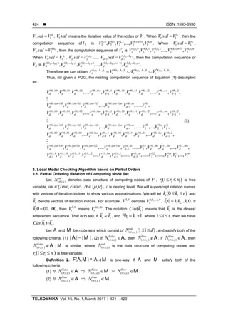
Definition 1. A partitioned dependency graph ( PDG ) is a tuple 1( , , ... , )nV E V V  ,
where V is a set of vertices, 2V
E V  is a set of hyper-edges, 1... nV V is a finite sequence of
subsets of V such that 1{ ,..., }nV V is a partition of V , and 1:{ ,..., } { , }nV V   is a
function that assigns  or  to each block of the partition [15]. Let { , }   . We shall
subsequently write ( )x  if ix V and ( )iV  .
G is a PDG, 1( , , ... , )nG V E V V  . Xinxin Liu, et al., [15] regarded G as a nested
boolean equation system [13], ( , ),i x S E y Sx V x y      . And ( )iV are nested in 1... nV V ,
where 1V and nV are the outermost block and innermost block respectively.

3. TELKOMNIKA ISSN: 1693-6930 
Local Model Checking Algorithm Based on Mu-calculus with Partial Orders (Hua Jiang)
423
Example 1. G is a PDG and 1 2 3 4( , , , )G V E VVVV  , where
1 2 3 4 5 6{ , , , , , }V x x x x x x , 1 1 2{ , }V x x , 2 3{ }V x , 3 4 5{ , }V x x , 4 6{ }V x ,
1 3 4 2 6 2 5 3 1 5 4 1 5 3 6 6 1{( ,{ , }),( ,{ }),( ,{ }),( ,{ , }),( ,{ }),( ,{ , }),( ,{ }),E x x x x x x x x x x x x x x x x x 6 4( ,{ })}x x ,
1( )V  , 2( )V  , 3( )V  , 4( )V  . Thus, the corresponding nested boolean
equation system consists of:
1 3 4
2 5 6
=x
:
x x
v
x x x


 
, 3 1 5:{x x x   ,
4 1
5 3 6
=x
:
x
v
x x x


 
, 6 1 4:{x x x  
2.2. Algorithm for PDG fixpoint Evaluatings
In reference [15] a local algorithm for evaluating PDG fixpoint, namely LAFP is
proposed, where the search space is constructed as a subset of V which is divided into three
blocks, and computes the fixpoints iteratively.
Given a PDG, let b denote the out-to-in sequence 1 2, ,..., db b b , where d
( mod 2 0d  ) is fixpoint nesting depth. There are in nodes in ib , and the fixpoint types are
2 1 2 1( )k kV    , 2 2( )k kV  , 1,2,...k  , respectively. So all the sequences of b are as
follows:
0
1
( 1)
1 1 10 11 1 1 1
2 2 20 21 2 2 2
1 1 ( 1)0 ( 1)1 ( 1) 1 1
0 1
: { , ,..., }, ( )
: { , ,..., }, ( )
: { , ,..., }, ( )
: { , ,...,
d
n
n
d d d d d n d d
d d d d dn
b V x x x V
b V x x x V
b V x x x V
b V x x x
 
 
       
 
 
 
 }, ( )d d dV 







 
(1)
Let’s divides iV into three blocks, denoting
' '' '''
i i i iV V V V   (1 )i d  , where
'
iV
saves nodes waiting for computing,
''
iV saves nodes which have been identified,
'''
iV saves
nodes which have not been identified. A assume that the initial value of state of each node of iV
are True or False, then 1( )V val True , 2( )V val False , 3( )V val True ,
4( )V val False , …, 1( )dV val True  , ( )dV val False respectively, ( )iV val means the
initial value of state of each node.
Let 1 2 1, ,..., ,d dg g g g be the computation function of the corresponding node of b in
PDG, then the iteration formulas is as follows:
1 1 1 1 1
1 2 1 1 2 1 2 1 2
1 2 1 1 2 1 1 2 11 1 2
1 2 1
1 ... ...
1 1 1 2 1
( 1) ... ..
2 2 1 2 1
...( 1) ... ...
1 1 1 2 1
... ( 1)
1
( , ,..., , )
( , ,..., , )
( , ,..., , )
(
d d d
d d
k k k k k
d d
k k k k k k k k k
d d
k k k k k k k k kk k k
d d d d
k k k k
d d
V g V V V V
V g V V V V
V g V V V V
V g V
    
 
  






  




 1 2 1 1 2 11 1 2 ... ...
2 1, ,..., , )d d dk k k k k k kk k k
d dV V V 
 (2)
The computing process of fixpoint nesting of LAFP is as follows. The computation
sequence of nodes of 1V is
0 1 2 1
1 1 1 1 1, , ,..., ,V V V V V 
. If 1V reaches the fixpoint with  , then

4.  ISSN: 1693-6930
TELKOMNIKA Vol. 15, No. 1, March 2017 : 421 – 429
424
1 1.V val V
 , 1.V val means the iteration value of the nodes of 1V . When 1
1 1. k
V val V , then the
computation sequence of 2V is 1 1 1 1 10 1 2 ( 1)
2 2 2 2 2, , ,..., ,k k k k k
V V V V V 
. When 1
1 1. k
V val V ,
1 2
2 2. k k
V val V , then the computation sequence of 3V is 1 2 1 2 1 2 1 2 1 20 1 2 ( 1)
2 2 2 2 2, , ,..., ,k k k k k k k k k k
V V V V V 
.
When 1
1 1. k
V val V , 1 2
2 2. k k
V val V ,…, 1 2 1...
1 1. dk k k
d dV val V 
  , then the computation sequence of
dV is 1 2 1 1 2 1 1 2 1 1 2 1 1 2 1... 0 ... 1 ... 2 ... ( 1) ...
, , ,..., ,d d d d dk k k k k k k k k k k k k k k
d d d d dV V V V V     
.
Therefore we can obtain 1 2 1 1 2 1 1 2 1 1 2 1... ... ... ...' '' '''i i i i i i i ik k k k k k k k k k k k k k k k
i i i iV V V V   
   .
Thus, for given a PDG, the nesting computation sequence of Equation (1) descripted
as:
00...00 00...01 00...02 00...0 00...1 00...10 00...11 00...12 00...1 00...2
1 1, , ,..., , , , , ,..., , ,d d d d d d d d d dV V V V V V V V V V 
 
00...( 1)0 00...( 1)1 00...( 1)2 00...( 1) 00... 01
1 2
01...00 01...01 01...02 01...0 01...1 01...10 01...11 01...12 01...1 01...2
1 1
, , ,..., , ,...... ,
, , ,..., , , , , ,..., , ,
d d d d d
d d d d d d d d d d
V V V V V V
V V V V V V V V V V
     
 
   

 
(3)
01...( 1)0 01...( 1)1 01...( 1)2 01...( 1) 01... 02 0 1
1 2 2 1
10...00 10...01 10...02 10...0 10...1 10...10 10...11 10...12 10...1 10..
1 1
, , ,..., , ,...... ,..., , ,
, , ,... , , , , ,... ,
d d d d d
d d d d d d d d d d
V V V V V V V V
V V V V V V V V V V
      
 
   

 
.2
,
10...( 1)0 10...( 1)1 10...( 1)2 10...( 1) 10... 11 11...00 11...01 11...0
1 2
11...1 11...10 11...11 11...12 11...1 11...2 11...
1 1 1
, , ,..., , ,...... , , ,..., ,
, , , ,..., , ,......, ,
d d d d d d d d
d d d d d d d
V V V V V V V V V
V V V V V V V
      
 
   

  
12 1 2
2 2 1 1...... ,......, , ,...,V V V V 
3. Local Model Checking Algorithm based on Partial Orders
3.1. Partial Ordering Relation of Computing Node Set
Let ( , , )i
val
i rN  denotes data structure of computing nodes of V , (1 )i i ir r n  is free
variable, { , }val True False , { , }   , i is nesting level. We will superscript relation names
with vectors of iteration indices to show various approximations. We will let (0 )i ik k n  and
ik denote vectors of iteration indices. For example,
0ik
iV denotes 1 2... 0ik k k
iV , 1 20 ... 0i ik k k k . If
0 00...00ik  , then
0ik
iV means
00...00
iV . The notation ( )tCas k means that tk is the closest
antecedent sequence. That is to say, if t tk h , and 1i ih k   , where 1 i t  , then we have
( )=t tCas h k .
Let A and M be node sets which consist of ( , , )(1 )i
val
i rN i d   , and satisfy both of the
following criteria, (1) | | = | |A M . (2) if ( , , )i
False
i rN A, then ( , , )i
True
i rN A. if ( , , )i
True
i rN A, then
( , , )i
False
i rN A；M is similar. where ( , , )i
val
i rN  is the data structure of computing nodes and
(1 )i i ir r n  is free variable.
Definition 2. F(A,M)= A M is one-way, if A and M satisfy both of the
following criteria
(1) ( , , ) ( , , ) ( , , )i i i
False False True
i r i r i rN N N       A M M .
(2) ( , , ) ( , , )i i
True True
i r i rN N    A M .

5. TELKOMNIKA ISSN: 1693-6930 
Local Model Checking Algorithm Based on Mu-calculus with Partial Orders (Hua Jiang)
425
Clearly, F satisfies reflexive, antisymmetrical and transitive, that is to say, F is a
partial ordering relation of computing node set.
For the iteration formulas (2), when 1
1 1. k
V val V , 1 2
2 2. k k
V val V ,…, 1 2 1...
1 1. dk k k
d dV val V 
 
, then the computation sequence of dV is
1 2 1 1 2 1 1 2 1 1 2 1 1 2 1... 0 ... 1 ... 2 ... ( 1) ...
, , ,..., ,d d d d dk k k k k k k k k k k k k k k
d d d d dV V V V V     
；
Because ( )d dV  , the val of each node of dV is False orTrue . If val is
changed from False toTrue , then storing the corresponding node of val in
''
dV . If
1 2 1 1 2 1 1 2 1 1 2 1 1 2 1... 0 ... 1 ... 2 ... ( 1) ...
, , ,..., ,d d d d dk k k k k k k k k k k k k k k
d d d d dV V V V V     
never change, by the Definition 4.2,
the sequence satisfies the formulas F , that is to say, the sequence is one-way, at the same
time, 1 2 1, ,..., ,d dg g g g is monotonous, then:
1 2 1 1 2 1 1 2 1 1 2 1 1 2 1... 0 ... 1 ... 2 ... ( 1) ...
...d d d d dk k k k k k k k k k k k k k k
d d d d d dV V V V V     
F : ；
For 1 1( )d dV    , we have:
1 2 2 1 2 2 1 2 2 1 2 2 1 2 2... ... ( 1) ... ( 2) ... 1 ... 0
1 1 1 1 1 1...d d d d dk k k k k k k k k k k k k k k
d d d d d dV V V V V       
     F : ； (4)
For 2 2( )V  , we have 1 1 1 1 10 1 2 ( 1)
2 2 2 2 2 2...k k k k k
V V V V V 
F : ；
For 1 1( )V  , we have
( 1) ( 2) 1 0
1 1 1 1 1 1...V V V V V   
F : .
Definition 3. 1 2... tk k k and 1 2... thh h are non-negative integer sequence, and both of
them have t integers. 1 2... tk k k is antecedent than 1 2... thh h , if they satisfy both of the following
criteria:
(1) Exiting an odd (even) bit j of 1 2... tk k k and 1 2... thh h , s.t. j jk h , where
1 , mod 2 0j t j   .
(2) m mk h , where 1 m t  , m j ；
1 2... tk k k is antecedent than 1 2... thh h , denoted 1 2... tk k k 1 2... thh h ； 1 2... tk k k
1 2... thh h denotes that 1 2... tk k k
iV has been computed when 1 2... th h h
iV is computed.
Definition 4. 1 2... tk k k is the antecedent sequence of 1 2... thh h , if they satisfy both of the
following criteria:
(1) 1 2... tk k k 1 2... thh h . (2) 1i ih k   , where 1 i t  ；
1 2... tk k k is the closest antecedent sequence of 1 2... thh h , denoting 1 2( ... )tCas hh h =
1 2... tk k k .
Lemma 1 If i  , 1 2( ... )tCas hh h = 1 2... tk k k , then 1 2... ih h h
iV and 1 2... ik k k
iV satisfy F ,
denoting 1 2... ih h h
iV 1 2... ik k k
iV .
Proof. (abbreviated)
Definition 5. 1 2,..., tk k k is an generalized antecedent sequence of 1 2,..., thh h , if they
satisfy both of the following criteria:
(1) The even sequence of 1 2,..., tk k k is equal to the even sequence of 1 2,..., thh h ,
denoting 1 2 1 2( ,..., ) ( ,..., )t tes k k k es hh h . (2) The odd sequence of 1 2,..., tk k k and the odd

6.  ISSN: 1693-6930
TELKOMNIKA Vol. 15, No. 1, March 2017 : 421 – 429
426
sequence of 1 2,..., thh h satisfy the lexicographic order, denoting
1 2 1 2( ( ,..., )) ( ( ,..., ))t tlo os k k k lo os hh h .
1 2,..., tk k k is an generalized antecedent sequence of 1 2,..., thh h , denoting
( )t tGas h k , where tk is 1 2,..., tk k k and th is 1 2,..., thh h .
Lemma 2. If i  , ( )t tGas h k , then ik
iV and ih
iV satisfy F , denoted i ih k
i iV V .
Proof. (abbreviated)
3.2. Local Model Checking Algorithm based on Partial Orders
As described above, LAFP presents an efficient local model checking algorithm,
however, in the nested process, inner value of fixpoint is affected by outer value of fixpoint. If
the value of outer iteration does not change, then the outer value of fixpoint starts computing
with the value of inner iteration. When the value of outer iteration is changed, then all the inner
value need to update, that is to say, a lot of computing processes is repeated.
For arbitrary sequence ik , i mod 2 = 1, by Lemma 1 and Lemma 2, we only need to
start the computing from the antecedent sequence ( )iCas k without affecting the correctness of
result. Thus, let
( )i ik Cas k
i iV V instead of ik
iV True , then the iteration time can be reduced
and the computing efficiency can be improved. The Local Model Checking Algorithm based on
Partial Orders is as follows:
Algorithm 1 Local Model Checking Algorithm based on Partial Orders
1. for ( i = 1; i <= d; i ++ ) do
2.
' '' '''
i i i iV V V V  ， ， ；// initialize
3. end for
4. i = d; // begin to compute from the innermost layer
5. while ( i > 0 ) do
6. if ( i == d ) then
7. Do
8. dequeue a node
*
iV from
'
iV ;
9.
' ' *
i i iV V V  ; //remove
*
iV
10. 1 1 1 111
1 1 1( ,..., , , )i i i i i i ik k k k k k nk
i i i i iV g V V V V 
 
- - -
=（ ）
;
11. if ( val of 1 1i ik k
iV -（ ）
changed ) then
12.
'' '' *
i i iV V V  ;
13. else
'' '' *
i i iV V V  ;
14. end if
15. until
'
iV ;
16. i = i -1;
17. end if
18. if ( i != d ) then
19. Do
20. dequeue a node
*
iV from
'
iV ;
21.
' ' *
i i iV V V  ;
22. 1 1 1 111
1 1 1( ,..., , , )i i i i i i ik k k k k k nk
i i i i iV g V V V V 
 
- - -
=（ ）
;
23. if ( val of 1 1i ik k
iV -（ ）
changed ) then
24.
'' '' *
i i iV V V  ;

7. TELKOMNIKA ISSN: 1693-6930 
Local Model Checking Algorithm Based on Mu-calculus with Partial Orders (Hua Jiang)
427
25. for ( t > i && t <= d ) do // update the value of all the inner layer
26. if ( t % 2 == 0 ) then
27. 0tk
tV False ; // the initial value is False
28. else if ( ( 0) 0ios k  ) then
29. 0tk
tV True ; // the initial value is True
30. else
0 ( )t tk Cas k
t tV V 
 ; //the initial value is
( )tCas k
tV 
31. end if
32. end if
33. end for
34. else
'' '' *
i i iV V V  ;
35. end if
36. until
'
iV ;
37. i = i – 1;
38. end if
39. end while
3.3. Time Complexity Analysis
When 1i  , according to 3.2, the computation sequence of the corresponding node is
0 1 2
1 1 1 1, , ,...,V V V V
in block 1b , 1n is the total number of computing node of block 1b . The initial
value of val is True in each node by 1 1( )V  . When the value of val turns into False
from True, by the monotonicity of function 1g , the value of the node no longer changes in the
whole computing process, so the node is deposited in
''
1V . The worst case is that the value of
val turns into False from True after computing each node of
'
1V , so the greatest computing
times of corresponding node in block 1b are
2
1 1 1| | 1 2 ...g n n     .
When 2i  , 1.V val = 1
1
k
V , the computation sequence of the corresponding node is
1 1 1 10 1 2
2 2 2 2, , ,...,k k k k
V V V V 
in block 2b , the computing times of the corresponding node are
21 2 3 ... n    in block 2b , the number of different values of 1.V val is 1n , so the greatest
computing times of corresponding node in block 2b are
2
2 1 2 1 2| | (1 2 3 ... )g n n n n       .
When 3i  , according to Algorithm 1, if 1 0k  , 3 0k  , 3V starts to compute from
'
3V .
In this case, the times are 2n at most. The changing times of corresponding node value are
2 3n n in block 3b , and the computing times are not more than
2
2 3n n . When 1 0k  , 3 0k  , 3V
starts to compute from 1 2 3
3
x x x
V . In this case, the times are 1 2nn at most, when it reaches the
fixpoint, the computing times are 1 2 3nn n at most, so the greatest computing times of
corresponding node in block 3b are
2
3 2 3 1 2 3| |g n n n n n     .
Summarily, when 2i  ,
2
2 2 4 6 2 2 2 1 2| | ...i i i ig n n n n n n  ,
2
2 1 2 4 6 2 2 1 2 4 6 2 1 2 2 1| | ... ...i i i i i ig n n n n n n n n n n n                .
Thus, we have 1 2
1
| | | | | | ...| |
d
i d
i
g g g g

  
2 2 2 2 2
1 1 2 2 3 1 2 3 2 3 4 2 4 5 2 3 4 5( ) ( ) ...n n n n n n n n n n n n n n n n n n                   

8.  ISSN: 1693-6930
TELKOMNIKA Vol. 15, No. 1, March 2017 : 421 – 429
428
2 2
2 4 6 2 1 2 4 6 3 2 1 2 4 6 2 1( ... ... ) ...d d d d d d d dn n n n n n n n n n n n n n n n n                  
2
2 4 6 2... | |dn n n n V      /2 2 2 /2+2
(2 ( / 2)/ ) | | = ( )d d
n d d V O d n     .
Assume the alternative nesting depth mod 2 0d  , through the analysis of the
above, then the time complexity analysis Algorithm 1 is
2 /2+2
( )d
O d n .
3.4. Space Complexity Analysis
By Algorithm 1, if ( )=i iV  , 1 2 2 1 1 2 2 1...( +1) 0 ...
=i i i ix x x x x x x x
i iV V    
, then save intermediate
results,
'
iV and
''
iV (1 )i d  account for 2d storage units. When 3i  , it accounts for 22n
storage units. When 5i  , it accounts for 2 42n n storage units. When i d , it accounts for
2 4 62 ... dn n n n    storage units, therefore, the total numbers of storage units in Algorithm 1
are:
2d + 22n + 2 42n n +…+ 2 4 62 ... dn n n n    2 2 4 2 4 62( ... ... )dd n n n n n n n         
/2 /2 /2 /2 /2
2( | | | | ... | | ) 2( / 2(| | )) ( ( ) )d d d d d
d V V V d d V O d d n         
3.5. Comparison of Time Complexity
According to Algorithm 1, we assume that the number of node of each layer is 30, then
we can obtain the time of iterative computation of all functions by computing. When the
alternation depth d takes a different value, the number of iteration is as Table 1. Table 1 shows
that our algorithm is more efficient.
Table 1. Times of Fuction Iterative Computing
d Algorithm 1 LAFP [15]
1 9.61*102
9.61*102
2 3.07*104
3.07*104
3 9.54*105
9.54*105
4 2.80*106
2.97*107
5 6.01*107
9.15*108
6 1.75*108
2.84*1010
7 6.62*109
8.81*1011
8 1.21*1010
2.74*1013
4. Conclusion
In this paper, we present a new efficient algorithm for evaluating PDG fixpoints. As we
know, [26] presented a local model checker forμ-calculus, as a tableau system, but it did not
analyze the computational complexity. Then [15] presented a new local algorithm for evaluating
PDG fixpoints, and time complexity of the LAFP algorithm was exponential relationship with
nesting depth. After a detailed analysis, we present a new algorithm by[11]. And our algorithm
takes about
2 /2+2d
d n steps. Clearly, the time required by our algori thm is only about the
square root of the time required by LAFP algorithm. Furthermore, when mod 2 1d  , we only
need to design the algorithm in the same way as mod 2 0d  . The nested bound algorithm
reduces repetitive computation and improves the computational efficiency. The research in this
paper is very important to theoretical research and practical application [25, 27], it can improve
the efficiency for verifying hardware and software designs.
As we know, two groups of partial ordered relation were presented by Tarski fixpoint
theory, our next work is to design a local algorithm by obtaining two groups of partial ordered
relation and improve the space complexity.

9. TELKOMNIKA ISSN: 1693-6930 
Local Model Checking Algorithm Based on Mu-calculus with Partial Orders (Hua Jiang)
429
Acknowledgements
This paper is supported by the National Natural Science Foundation of China under
Grant No.61472406, the Natural Science Foundation of Fujian Province under Grant
No.2015J01269 and No.2016J01304 and the Talent Introduction Foundation of Minnan Normal
University.
References
[1] D Kozen. Results on the propositional μ-calculus. LNCS 140: Proc of the 9
th
Colloquium on
Automata, Languages and Programming. Springer. 1982: 348-359.
[2] JW de Bakker. Mathematical theory of program correctness. Prentice-Hall, Inc. 1980.
[3] D Park. Fixpoint induction and proof of program semantics. In: B Meltzer, D Michie. Editors. Mach.
Int, Edinburgh Univ. 1970: 59-78.
[4] C Stirling. Modal and temporal logics for processes. Springer. 1996: 149-237.
[5] A Tarski. A lattice-theoretical fixpoint theorem and its applications. Pacific Journal of Mathematics.
1955; 5(2): 285-309.
[6] EA Emerson, CL Lei. Efficient model checking in fragments of the propositional mu-calculus. Proc.
1st LICS. 1986.
[7] HR Andersen. Model checking and boolean graphs. ESOP 92. Springer. 1992: 1-19.
[8] R Cleaveland, M Klein, B Steen. Faster model checking for the modal mu-calculus. CAV 92, LNCS.
1992; 663: 410-422.
[9] R Cleaveland. Tableau-based model checking in the prepositional mucalculus. Acta Informatica.
1990; 27(8): 725-747.
[10] DE Long, A Browne, EM Clarke, et al. An improved algorithm for the evaluation of fixpoint
expressions. Computer Aided Verification. 1994: 338-350.
[11] H Jiang. Efficient global model-checking for propositional μ-calculus. Journal of Computer Research
and Development. 2010; 47(8): 1424-1433.
[12] HR Andersen. Model checking and boolean graphs. Theoretical Computer Science. 1994; 126(1).
[13] B Vergauwen, J Lewi. Efficient local correctness checking for single and alternating boolean equation
systems. Proceedings of ICALP 94. Springer. 1994: 304-315.
[14] GS Bhat, R Cleaveland. Efficient model checking for fragments of the modal μ-calculus. Proceedings
of the Second International Workshop on Tools and Algorithms for the Construction and Analysis of
Systems (TACAS 96). Springer. 1996: 107-126.
[15] XX Liu, CR Ramakrishnan, SA Smolka. Fully local and efficient evaluation of alternating fixed points.
Tools and Algorithms for the Construction and Analysis of Systems. 1998: 5-19.
[16] R Mateescu. Local model-checking of modal mu-calculus on acyclic labeled transition systems. Tools
and Algorithm for the Construction and Analysis of Systems. 2002: 281-295.
[17] JF Jensen, LK Østergaard. Local model checking of weighted CTL. 2012.
[18] D Latella, M Loreti, M Massink. On-the-fly fast mean-field modelchecking. Trustworthy Global
Computing. Springer International Publishing, LNCS. 2014: 297-314.
[19] R Guerraoui, M Yabandeh. Local model checking. 2011.
[20] JF Jensen, KG Larsen, J Srba, et al. Local model checking of weighted CTL with upper-bound
constraints. Model Checking Software. 2013: 178-195.
[21] Hua Jiang, Jianqing Xi. Improved algorithm of golbal model-checking for propositional mu-calculus.
Applied Mechanics and Materials. 2013; 263: 2314-2319.
[22] Liu Wanwei, et al. A Simple Probabilistic Extension of Modal Mu-calculus. 2015.
[23] Castro Pablo, Cecilia Kilmurray, Nir Piterman. Tractable Probabilistic μ-Calculus that Expresses
Probabilistic Temporal Logics. 2015.
[24] EM Clarke, O Grumberg, D Peled. Model checking. MIT Press. 1999.
[25] N Piterman, MY Vardi. Global model-checking of infinite-state systems. Computer Aided Verification.
2004: 387-400.
[26] C Stirling, D Walker. Local model checking in the modal mu-calculus. Theoretical Computer Science.
1991; 89(1): 161-177.
[27] T Schuele, K Schneider. Global vs. local model checking of infinite state systems. MBMV. 2004: 54-
64.