Download as PDF, PPTX


![Population Structure
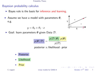
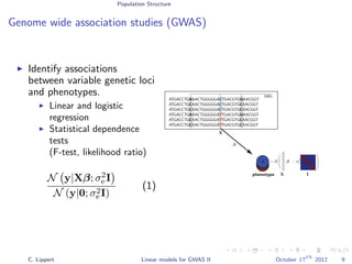
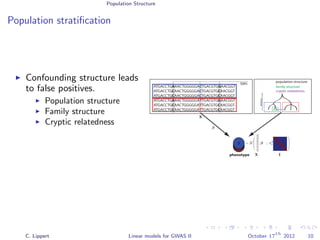
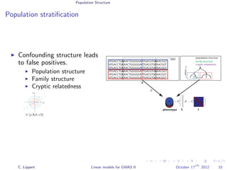
Population stratification
GWA on inflammatory bowel disease (WTCCC)
3.4k cases, 11.9k controls
Methods
Linear regression
Likelihood ratio test
[Burton et al., 2007]
C. Lippert Linear models for GWAS II October 17
th
2012 11](https://image.slidesharecdn.com/linearmodels2-200808124746/85/Linear-models2-32-320.jpg)
![Population Structure
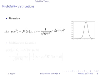
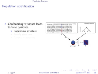
Population stratification
GWA on inflammatory bowel disease (WTCCC)
3.4k cases, 11.9k controls
Methods
Linear regression
Likelihood ratio test
[Burton et al., 2007]
C. Lippert Linear models for GWAS II October 17
th
2012 11](https://image.slidesharecdn.com/linearmodels2-200808124746/85/Linear-models2-33-320.jpg)
![Population Structure
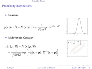
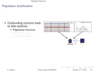
Population stratification
GWA on inflammatory bowel disease (WTCCC)
3.4k cases, 11.9k controls
Methods
Linear regression
Likelihood ratio test
[Burton et al., 2007]
C. Lippert Linear models for GWAS II October 17
th
2012 11](https://image.slidesharecdn.com/linearmodels2-200808124746/85/Linear-models2-34-320.jpg)
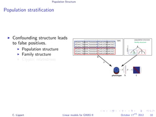
![Population structure correction
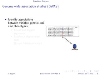
Genomic control [Devlin and Roeder, Biometrics 1999]
Genomic control λ
λ =
median(2LR)
median(χ2)
.
λ = 1: Calibrated
P-values
λ > 1: Inflation
λ < 1: Deflation
Correct by dividing test
statistic by λ.
Applicable in combination
with every method.
Does not change
(non-)uniformity of
P-values.
Very conservative.C. Lippert Linear models for GWAS II October 17
th
2012 13](https://image.slidesharecdn.com/linearmodels2-200808124746/85/Linear-models2-36-320.jpg)
![Population structure correction
Genomic control [Devlin and Roeder, Biometrics 1999]
Genomic control λ
λ =
median(2LR)
median(χ2)
.
λ = 1: Calibrated
P-values
λ > 1: Inflation
λ < 1: Deflation
Correct by dividing test
statistic by λ.
Applicable in combination
with every method.
Does not change
(non-)uniformity of
P-values.
Very conservative.C. Lippert Linear models for GWAS II October 17
th
2012 13](https://image.slidesharecdn.com/linearmodels2-200808124746/85/Linear-models2-37-320.jpg)
![Population structure correction
Genomic control [Devlin and Roeder, Biometrics 1999]
Genomic control λ
λ =
median(2LR)
median(χ2)
.
λ = 1: Calibrated
P-values
λ > 1: Inflation
λ < 1: Deflation
Correct by dividing test
statistic by λ.
Applicable in combination
with every method.
Does not change
(non-)uniformity of
P-values.
Very conservative.C. Lippert Linear models for GWAS II October 17
th
2012 13](https://image.slidesharecdn.com/linearmodels2-200808124746/85/Linear-models2-38-320.jpg)
![Population structure correction
Genomic control [Devlin and Roeder, Biometrics 1999]
Genomic control λ
λ =
median(2LR)
median(χ2)
.
λ = 1: Calibrated
P-values
λ > 1: Inflation
λ < 1: Deflation
Correct by dividing test
statistic by λ.
Applicable in combination
with every method.
Does not change
(non-)uniformity of
P-values.
Very conservative.C. Lippert Linear models for GWAS II October 17
th
2012 13](https://image.slidesharecdn.com/linearmodels2-200808124746/85/Linear-models2-39-320.jpg)
![Population structure correction
Genomic control [Devlin and Roeder, Biometrics 1999]
Genomic control λ
λ =
median(2LR)
median(χ2)
.
λ = 1: Calibrated
P-values
λ > 1: Inflation
λ < 1: Deflation
Correct by dividing test
statistic by λ.
Applicable in combination
with every method.
Does not change
(non-)uniformity of
P-values.
Very conservative.C. Lippert Linear models for GWAS II October 17
th
2012 13](https://image.slidesharecdn.com/linearmodels2-200808124746/85/Linear-models2-40-320.jpg)
![Population structure correction
Genomic control [Devlin and Roeder, Biometrics 1999]
Genomic control λ
λ =
median(2LR)
median(χ2)
.
λ = 1: Calibrated
P-values
λ > 1: Inflation
λ < 1: Deflation
Correct by dividing test
statistic by λ.
Applicable in combination
with every method.
Does not change
(non-)uniformity of
P-values.
Very conservative.C. Lippert Linear models for GWAS II October 17
th
2012 13](https://image.slidesharecdn.com/linearmodels2-200808124746/85/Linear-models2-41-320.jpg)
![Population structure correction
Eigenstrat
Population structure causes
genome-wide correlations
between SNPs
A large part of the total
variation in the SNPs can be
explained by population
differences.
Novembre et al. [2008] show that the
eigenvectors of the SNP
covariance matrix reflect
population structure.
Eigenstrat uses this property
to correct for population
structure in GWAS.
[Price et al., 2006, Patterson et al., 2006, Novembre et al., 2008]
C. Lippert Linear models for GWAS II October 17
th
2012 14](https://image.slidesharecdn.com/linearmodels2-200808124746/85/Linear-models2-42-320.jpg)
![Population structure correction
Eigenstrat
Population structure causes
genome-wide correlations
between SNPs
A large part of the total
variation in the SNPs can be
explained by population
differences.
Novembre et al. [2008] show that the
eigenvectors of the SNP
covariance matrix reflect
population structure.
Eigenstrat uses this property
to correct for population
structure in GWAS.
[Price et al., 2006, Patterson et al., 2006, Novembre et al., 2008]
C. Lippert Linear models for GWAS II October 17
th
2012 14](https://image.slidesharecdn.com/linearmodels2-200808124746/85/Linear-models2-43-320.jpg)
![Population structure correction
Eigenstrat
Population structure causes
genome-wide correlations
between SNPs
A large part of the total
variation in the SNPs can be
explained by population
differences.
Novembre et al. [2008] show that the
eigenvectors of the SNP
covariance matrix reflect
population structure.
Eigenstrat uses this property
to correct for population
structure in GWAS.
[Price et al., 2006, Patterson et al., 2006, Novembre et al., 2008]
C. Lippert Linear models for GWAS II October 17
th
2012 14](https://image.slidesharecdn.com/linearmodels2-200808124746/85/Linear-models2-44-320.jpg)
![Population structure correction
Eigenstrat
Population structure causes
genome-wide correlations
between SNPs
A large part of the total
variation in the SNPs can be
explained by population
differences.
Novembre et al. [2008] show that the
eigenvectors of the SNP
covariance matrix reflect
population structure.
Eigenstrat uses this property
to correct for population
structure in GWAS.
[Price et al., 2006, Patterson et al., 2006, Novembre et al., 2008]
C. Lippert Linear models for GWAS II October 17
th
2012 14](https://image.slidesharecdn.com/linearmodels2-200808124746/85/Linear-models2-45-320.jpg)
![Population structure correction
Eigenstrat
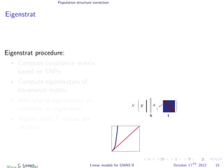
Eigenstrat procedure:
Compute covariance matrix
based on SNPs
Compute eigenvectors of
covariance matrix
Add largest eigenvector as
covariate to regression.
Repeat until P-values are
uniform.
X − E [X]
N β
X
C
C
C
T
T
T
Genome-wide SNP covariance
C. Lippert Linear models for GWAS II October 17
th
2012 15](https://image.slidesharecdn.com/linearmodels2-200808124746/85/Linear-models2-47-320.jpg)
![Population structure correction
Eigenstrat
Eigenstrat procedure:
Compute covariance matrix
based on SNPs
Compute eigenvectors of
covariance matrix
Add largest eigenvector as
covariate to regression.
Repeat until P-values are
uniform.
X − E [X]
N β
X
C
C
C
T
T
T
Genome-wide SNP covariance
Eigenvectors Eigenvalues
C. Lippert Linear models for GWAS II October 17
th
2012 15](https://image.slidesharecdn.com/linearmodels2-200808124746/85/Linear-models2-48-320.jpg)
![Population structure correction
Eigenstrat
Eigenstrat procedure:
Compute covariance matrix
based on SNPs
Compute eigenvectors of
covariance matrix
Add largest eigenvector as
covariate to regression.
Repeat until P-values are
uniform.
X − E [X]
N β
X
C
C
C
T
T
T
Genome-wide SNP covariance
Eigenvectors Eigenvalues
Add as covariates
C. Lippert Linear models for GWAS II October 17
th
2012 15](https://image.slidesharecdn.com/linearmodels2-200808124746/85/Linear-models2-49-320.jpg)
![Population structure correction
Eigenstrat
Eigenstrat procedure:
Compute covariance matrix
based on SNPs
Compute eigenvectors of
covariance matrix
Add largest eigenvector as
covariate to regression.
Repeat until P-values are
uniform.
X − E [X]
N β
X
C
C
C
T
T
T
Genome-wide SNP covariance
Eigenvectors Eigenvalues
Add as covariates
C. Lippert Linear models for GWAS II October 17
th
2012 15](https://image.slidesharecdn.com/linearmodels2-200808124746/85/Linear-models2-50-320.jpg)

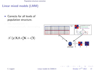

![Population structure correction
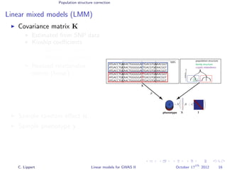
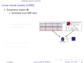
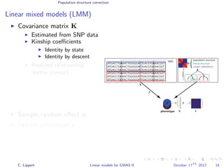
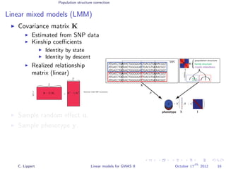
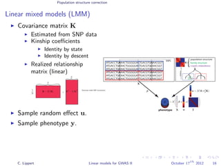
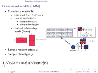
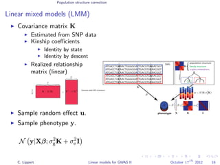
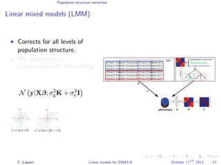
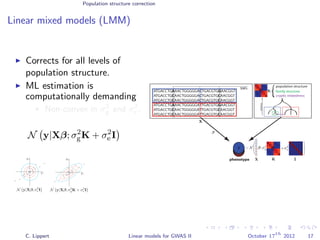
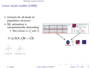
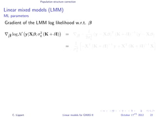
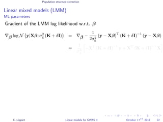
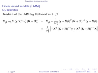
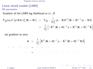
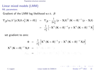
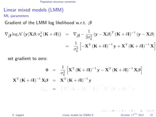
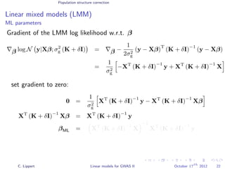
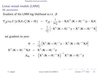
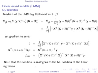
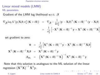
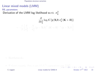
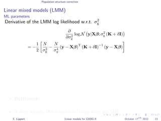
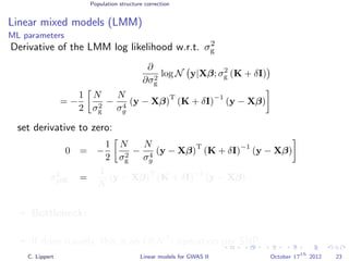
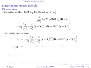
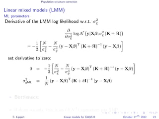
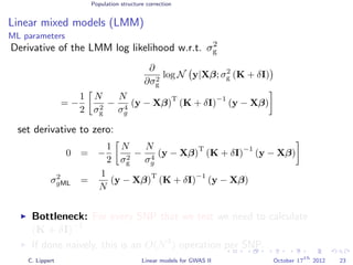
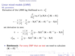
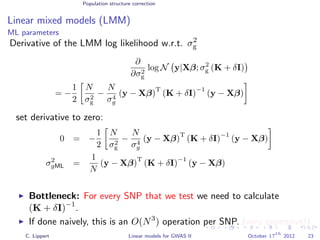
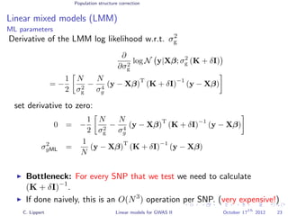
Linear mixed models (LMM)
LMM log likelihood
LL(β, σ2
g, σ2
e ) = log N y|Xβ; σ2
gK + σ2
e I .
Change of variables, introducing δ = σ2
e /σ2
g:
LL(β, σ2
g, δ) = log N y|Xβ; σ2
g (K + δI) .
ML-parameters ˆβ and ˆσ2
g follow in closed form.
Use optimizer to solve 1-dimensional optimization problem over δ.
[Kang et al., 2008]
C. Lippert Linear models for GWAS II October 17
th
2012 21](https://image.slidesharecdn.com/linearmodels2-200808124746/85/Linear-models2-67-320.jpg)
![Population structure correction
Linear mixed models (LMM)
LMM log likelihood
LL(β, σ2
g, σ2
e ) = log N y|Xβ; σ2
gK + σ2
e I .
Change of variables, introducing δ = σ2
e /σ2
g:
LL(β, σ2
g, δ) = log N y|Xβ; σ2
g (K + δI) .
ML-parameters ˆβ and ˆσ2
g follow in closed form.
Use optimizer to solve 1-dimensional optimization problem over δ.
[Kang et al., 2008]
C. Lippert Linear models for GWAS II October 17
th
2012 21](https://image.slidesharecdn.com/linearmodels2-200808124746/85/Linear-models2-68-320.jpg)
![Population structure correction
Linear mixed models (LMM)
LMM log likelihood
LL(β, σ2
g, σ2
e ) = log N y|Xβ; σ2
gK + σ2
e I .
Change of variables, introducing δ = σ2
e /σ2
g:
LL(β, σ2
g, δ) = log N y|Xβ; σ2
g (K + δI) .
ML-parameters ˆβ and ˆσ2
g follow in closed form.
Use optimizer to solve 1-dimensional optimization problem over δ.
[Kang et al., 2008]
C. Lippert Linear models for GWAS II October 17
th
2012 21](https://image.slidesharecdn.com/linearmodels2-200808124746/85/Linear-models2-69-320.jpg)
![Population structure correction
Linear mixed models (LMM)
LMM log likelihood
LL(β, σ2
g, σ2
e ) = log N y|Xβ; σ2
gK + σ2
e I .
Change of variables, introducing δ = σ2
e /σ2
g:
LL(β, σ2
g, δ) = log N y|Xβ; σ2
g (K + δI) .
ML-parameters ˆβ and ˆσ2
g follow in closed form.
Use optimizer to solve 1-dimensional optimization problem over δ.
[Kang et al., 2008]
C. Lippert Linear models for GWAS II October 17
th
2012 21](https://image.slidesharecdn.com/linearmodels2-200808124746/85/Linear-models2-70-320.jpg)

![Population structure correction
FaST LMM
N y|Xβ; σ2
g (K + δI) .
[Lippert et al., 2011]
C. Lippert Linear models for GWAS II October 17
th
2012 24](https://image.slidesharecdn.com/linearmodels2-200808124746/85/Linear-models2-91-320.jpg)
![Population structure correction
FaST LMM
N y|Xβ; σ2
g (K + δI) .
= N y|Xβ; σ2
g USUT
+ δI .
[Lippert et al., 2011]
C. Lippert Linear models for GWAS II October 17
th
2012 24](https://image.slidesharecdn.com/linearmodels2-200808124746/85/Linear-models2-92-320.jpg)
![Population structure correction
FaST LMM
N y|Xβ; σ2
g (K + δI) .
= N y|Xβ; σ2
g USUT
+ δI .
= N UT
y|UT
Xβ; σ2
g UT
USUT
U + δUT
U .
[Lippert et al., 2011]
C. Lippert Linear models for GWAS II October 17
th
2012 24](https://image.slidesharecdn.com/linearmodels2-200808124746/85/Linear-models2-93-320.jpg)
![Population structure correction
FaST LMM
N y|Xβ; σ2
g (K + δI) .
= N y|Xβ; σ2
g USUT
+ δI .
= N
UT
y|UT
Xβ; σ2
g
UT
U
I
S UT
U
I
+δ UT
U
I
.
[Lippert et al., 2011]
C. Lippert Linear models for GWAS II October 17
th
2012 24](https://image.slidesharecdn.com/linearmodels2-200808124746/85/Linear-models2-94-320.jpg)
![Population structure correction
FaST LMM
N y|Xβ; σ2
g (K + δI) .
= N y|Xβ; σ2
g USUT
+ δI .
= N
UT
y|UT
Xβ; σ2
g
UT
U
I
S UT
U
I
+δ UT
U
I
.
= N UT
y|UT
Xβ; σ2
g (S + δI) .
[Lippert et al., 2011]
C. Lippert Linear models for GWAS II October 17
th
2012 24](https://image.slidesharecdn.com/linearmodels2-200808124746/85/Linear-models2-95-320.jpg)
![Population structure correction
FaST LMM
N y|Xβ; σ2
g (K + δI) .
= N y|Xβ; σ2
g USUT
+ δI .
= N
UT
y|UT
Xβ; σ2
g
UT
U
I
S UT
U
I
+δ UT
U
I
.
= N UT
y|UT
Xβ; σ2
g (S + δI) .
[Lippert et al., 2011]
C. Lippert Linear models for GWAS II October 17
th
2012 24](https://image.slidesharecdn.com/linearmodels2-200808124746/85/Linear-models2-96-320.jpg)
![Population structure correction
FaST LMM
N y|Xβ; σ2
g (K + δI) .
= N y|Xβ; σ2
g USUT
+ δI .
= N
UT
y|UT
Xβ; σ2
g
UT
U
I
S UT
U
I
+δ UT
U
I
.
= N UT
y|UT
Xβ; σ2
g (S + δI) .
[Lippert et al., 2011]
C. Lippert Linear models for GWAS II October 17
th
2012 24](https://image.slidesharecdn.com/linearmodels2-200808124746/85/Linear-models2-97-320.jpg)
![Population structure correction
FaST LMM
N UT
y|UT
Xβ; σ2
g (S + δI) . (2)
Factored Spectrally Transformed LMM
O(N3
) once for spectral decomposition.
O(N2
) runtime per SNP tested (multiplication with UT
).
O(N2
) memory for storing K and U.
[Lippert et al., 2011]
C. Lippert Linear models for GWAS II October 17
th
2012 25](https://image.slidesharecdn.com/linearmodels2-200808124746/85/Linear-models2-98-320.jpg)
![Population structure correction
FaST LMM
N UT
y|UT
Xβ; σ2
g (S + δI) . (2)
Factored Spectrally Transformed LMM
O(N3
) once for spectral decomposition.
O(N2
) runtime per SNP tested (multiplication with UT
).
O(N2
) memory for storing K and U.
[Lippert et al., 2011]
C. Lippert Linear models for GWAS II October 17
th
2012 25](https://image.slidesharecdn.com/linearmodels2-200808124746/85/Linear-models2-99-320.jpg)
![Population structure correction
FaST LMM
N UT
y|UT
Xβ; σ2
g (S + δI) . (2)
Factored Spectrally Transformed LMM
O(N3
) once for spectral decomposition.
O(N2
) runtime per SNP tested (multiplication with UT
).
O(N2
) memory for storing K and U.
[Lippert et al., 2011]
C. Lippert Linear models for GWAS II October 17
th
2012 25](https://image.slidesharecdn.com/linearmodels2-200808124746/85/Linear-models2-100-320.jpg)
![Population structure correction
FaST LMM
N UT
y|UT
Xβ; σ2
g (S + δI) . (2)
Factored Spectrally Transformed LMM
O(N3
) once for spectral decomposition.
O(N2
) runtime per SNP tested (multiplication with UT
).
O(N2
) memory for storing K and U.
[Lippert et al., 2011]
C. Lippert Linear models for GWAS II October 17
th
2012 25](https://image.slidesharecdn.com/linearmodels2-200808124746/85/Linear-models2-101-320.jpg)
![Population structure correction
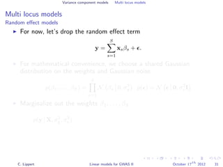
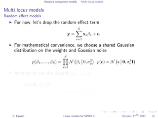
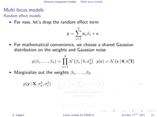
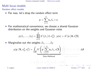
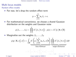
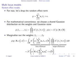
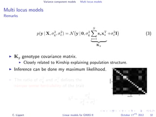
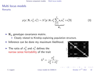
Multi locus models
Generalization to multiple genetic factors
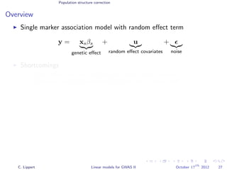
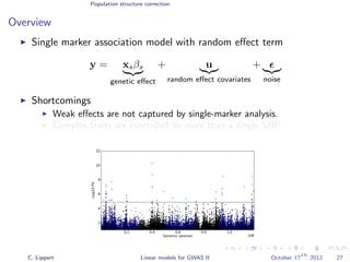
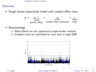
y =
S
s=1
xsβs
genetic effect
+ u
random effect covariates
+
noise
Challenge: N << S: explicit estimation of all βs is not feasible.
Solutions
Regularize βs (Ridge regression, LASSO)
Variance component modeling
[Wu et al., 2011]
C. Lippert Linear models for GWAS II October 17
th
2012 28](https://image.slidesharecdn.com/linearmodels2-200808124746/85/Linear-models2-108-320.jpg)
![Population structure correction
Multi locus models
Generalization to multiple genetic factors
y =
S
s=1
xsβs
genetic effect
+ u
random effect covariates
+
noise
Challenge: N << S: explicit estimation of all βs is not feasible.
Solutions
Regularize βs (Ridge regression, LASSO)
Variance component modeling
[Wu et al., 2011]
C. Lippert Linear models for GWAS II October 17
th
2012 28](https://image.slidesharecdn.com/linearmodels2-200808124746/85/Linear-models2-109-320.jpg)
![Population structure correction
Multi locus models
Generalization to multiple genetic factors
y =
S
s=1
xsβs
genetic effect
+ u
random effect covariates
+
noise
Challenge: N << S: explicit estimation of all βs is not feasible.
Solutions
Regularize βs (Ridge regression, LASSO)
Variance component modeling
[Wu et al., 2011]
C. Lippert Linear models for GWAS II October 17
th
2012 28](https://image.slidesharecdn.com/linearmodels2-200808124746/85/Linear-models2-110-320.jpg)
![Population structure correction
Multi locus models
Generalization to multiple genetic factors
y =
S
s=1
xsβs
genetic effect
+ u
random effect covariates
+
noise
Challenge: N << S: explicit estimation of all βs is not feasible.
Solutions
Regularize βs (Ridge regression, LASSO)
Variance component modeling
[Wu et al., 2011]
C. Lippert Linear models for GWAS II October 17
th
2012 28](https://image.slidesharecdn.com/linearmodels2-200808124746/85/Linear-models2-111-320.jpg)

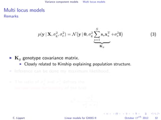
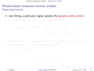
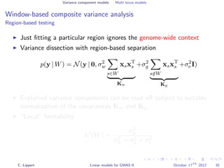
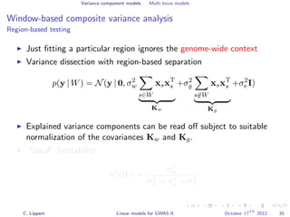
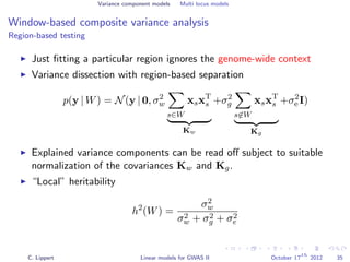
![Variance component models Multi locus models
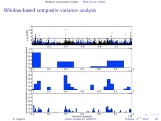
Window-based composite variance analysis
Significance testing
Analogously to fixed effect testing, the significance of a specific
window can be tested.
Likelihood-ratio statistics to score the relevance of a particular
genomic region W
LOD(W) =
N y 0, σ2
w s∈W xsxT
s + σ2
g s∈W xsxT
s + σ2
e I
N y 0, σ2
g s∈W xsxT
s + σ2
e I
P-values can be obtained from permutation statistics or analytical
approximation (variants of score tests or likelihood ratio tests).
[Wu et al., 2011, Listgarten et al., 2012]
C. Lippert Linear models for GWAS II October 17
th
2012 37](https://image.slidesharecdn.com/linearmodels2-200808124746/85/Linear-models2-131-320.jpg)
![Variance component models Multi locus models
Window-based composite variance analysis
Significance testing
Analogously to fixed effect testing, the significance of a specific
window can be tested.
Likelihood-ratio statistics to score the relevance of a particular
genomic region W
LOD(W) =
N y 0, σ2
w s∈W xsxT
s + σ2
g s∈W xsxT
s + σ2
e I
N y 0, σ2
g s∈W xsxT
s + σ2
e I
P-values can be obtained from permutation statistics or analytical
approximation (variants of score tests or likelihood ratio tests).
[Wu et al., 2011, Listgarten et al., 2012]
C. Lippert Linear models for GWAS II October 17
th
2012 37](https://image.slidesharecdn.com/linearmodels2-200808124746/85/Linear-models2-132-320.jpg)
![Variance component models Multi locus models
Window-based composite variance analysis
Significance testing
Analogously to fixed effect testing, the significance of a specific
window can be tested.
Likelihood-ratio statistics to score the relevance of a particular
genomic region W
LOD(W) =
N y 0, σ2
w s∈W xsxT
s + σ2
g s∈W xsxT
s + σ2
e I
N y 0, σ2
g s∈W xsxT
s + σ2
e I
P-values can be obtained from permutation statistics or analytical
approximation (variants of score tests or likelihood ratio tests).
[Wu et al., 2011, Listgarten et al., 2012]
C. Lippert Linear models for GWAS II October 17
th
2012 37](https://image.slidesharecdn.com/linearmodels2-200808124746/85/Linear-models2-133-320.jpg)
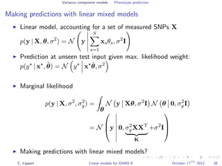
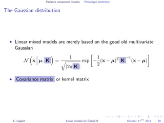
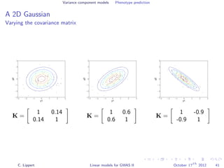
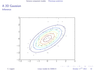
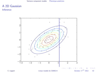
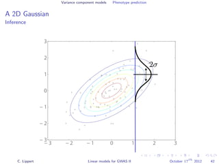
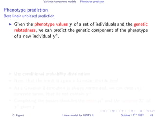
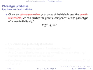
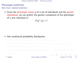
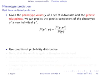
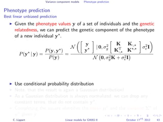
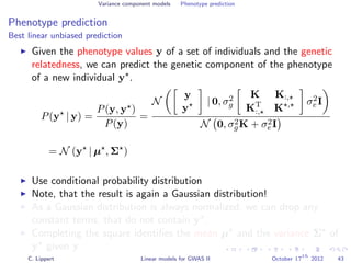
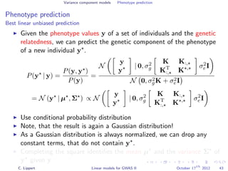
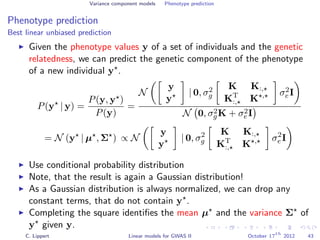
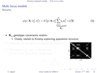
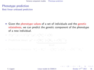
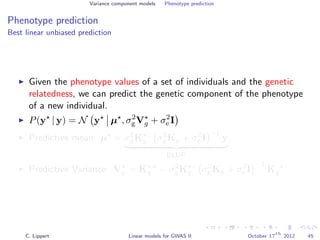
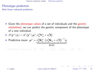
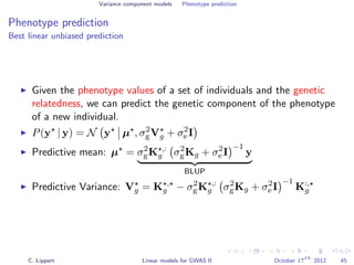
![Variance component models Phenotype prediction
Inference
Gaussian conditioning in 2D
p(y2 | y1, K) =
p(y1, y2 | K)
p(y1 | K)
∝ exp −
1
2
[y1, y2] K−1 y1
y2
= exp{−
1
2
y2
1K−1
1,1 + y2
2K−1
2,2 + 2y1K−1
1,2y2 }
= exp{−
1
2
y2
2K−1
2,2 + 2y2K−1
1,2y1 + C }
= Z exp{−
1
2
K−1
2,2 y2
2 + 2y2
K−1
1,2y1
K−1
2,2
}
= Z exp{−
1
2
K−1
2,2 y2
2 + 2y2
K−1
1,2y1
K−1
2,2
+
K−1
1,2y1
K−1
2,2
2
+
1
2
K−1
2,2
K−1
1,2y1
K−1
2,2
2
}
= Z exp{−
1
2
K−1
2,2
Σ
y2 +
K−1
1,2y1
K−1
2,2
−µ
2
} ∝ N (y2 | µ, Σ)
C. Lippert Linear models for GWAS II October 17
th
2012 44](https://image.slidesharecdn.com/linearmodels2-200808124746/85/Linear-models2-153-320.jpg)
![Variance component models Phenotype prediction
Inference
Gaussian conditioning in 2D
p(y2 | y1, K) =
p(y1, y2 | K)
p(y1 | K)
∝ exp −
1
2
[y1, y2] K−1 y1
y2
= exp{−
1
2
y2
1K−1
1,1 + y2
2K−1
2,2 + 2y1K−1
1,2y2 }
= exp{−
1
2
y2
2K−1
2,2 + 2y2K−1
1,2y1 + C }
= Z exp{−
1
2
K−1
2,2 y2
2 + 2y2
K−1
1,2y1
K−1
2,2
}
= Z exp{−
1
2
K−1
2,2 y2
2 + 2y2
K−1
1,2y1
K−1
2,2
+
K−1
1,2y1
K−1
2,2
2
+
1
2
K−1
2,2
K−1
1,2y1
K−1
2,2
2
}
= Z exp{−
1
2
K−1
2,2
Σ
y2 +
K−1
1,2y1
K−1
2,2
−µ
2
} ∝ N (y2 | µ, Σ)
C. Lippert Linear models for GWAS II October 17
th
2012 44](https://image.slidesharecdn.com/linearmodels2-200808124746/85/Linear-models2-154-320.jpg)
![Variance component models Phenotype prediction
Inference
Gaussian conditioning in 2D
p(y2 | y1, K) =
p(y1, y2 | K)
p(y1 | K)
∝ exp −
1
2
[y1, y2] K−1 y1
y2
= exp{−
1
2
y2
1K−1
1,1 + y2
2K−1
2,2 + 2y1K−1
1,2y2 }
= exp{−
1
2
y2
2K−1
2,2 + 2y2K−1
1,2y1 + C }
= Z exp{−
1
2
K−1
2,2 y2
2 + 2y2
K−1
1,2y1
K−1
2,2
}
= Z exp{−
1
2
K−1
2,2 y2
2 + 2y2
K−1
1,2y1
K−1
2,2
+
K−1
1,2y1
K−1
2,2
2
+
1
2
K−1
2,2
K−1
1,2y1
K−1
2,2
2
}
= Z exp{−
1
2
K−1
2,2
Σ
y2 +
K−1
1,2y1
K−1
2,2
−µ
2
} ∝ N (y2 | µ, Σ)
C. Lippert Linear models for GWAS II October 17
th
2012 44](https://image.slidesharecdn.com/linearmodels2-200808124746/85/Linear-models2-155-320.jpg)
![Variance component models Phenotype prediction
Inference
Gaussian conditioning in 2D
p(y2 | y1, K) =
p(y1, y2 | K)
p(y1 | K)
∝ exp −
1
2
[y1, y2] K−1 y1
y2
= exp{−
1
2
y2
1K−1
1,1 + y2
2K−1
2,2 + 2y1K−1
1,2y2 }
= exp{−
1
2
y2
2K−1
2,2 + 2y2K−1
1,2y1 + C }
= Z exp{−
1
2
K−1
2,2 y2
2 + 2y2
K−1
1,2y1
K−1
2,2
}
= Z exp{−
1
2
K−1
2,2 y2
2 + 2y2
K−1
1,2y1
K−1
2,2
+
K−1
1,2y1
K−1
2,2
2
+
1
2
K−1
2,2
K−1
1,2y1
K−1
2,2
2
}
= Z exp{−
1
2
K−1
2,2
Σ
y2 +
K−1
1,2y1
K−1
2,2
−µ
2
} ∝ N (y2 | µ, Σ)
C. Lippert Linear models for GWAS II October 17
th
2012 44](https://image.slidesharecdn.com/linearmodels2-200808124746/85/Linear-models2-156-320.jpg)
![Variance component models Phenotype prediction
Inference
Gaussian conditioning in 2D
p(y2 | y1, K) =
p(y1, y2 | K)
p(y1 | K)
∝ exp −
1
2
[y1, y2] K−1 y1
y2
= exp{−
1
2
y2
1K−1
1,1 + y2
2K−1
2,2 + 2y1K−1
1,2y2 }
= exp{−
1
2
y2
2K−1
2,2 + 2y2K−1
1,2y1 + C }
= Z exp{−
1
2
K−1
2,2 y2
2 + 2y2
K−1
1,2y1
K−1
2,2
}
= Z exp{−
1
2
K−1
2,2 y2
2 + 2y2
K−1
1,2y1
K−1
2,2
+
K−1
1,2y1
K−1
2,2
2
+
1
2
K−1
2,2
K−1
1,2y1
K−1
2,2
2
}
= Z exp{−
1
2
K−1
2,2
Σ
y2 +
K−1
1,2y1
K−1
2,2
−µ
2
} ∝ N (y2 | µ, Σ)
C. Lippert Linear models for GWAS II October 17
th
2012 44](https://image.slidesharecdn.com/linearmodels2-200808124746/85/Linear-models2-157-320.jpg)
![Variance component models Phenotype prediction
Inference
Gaussian conditioning in 2D
p(y2 | y1, K) =
p(y1, y2 | K)
p(y1 | K)
∝ exp −
1
2
[y1, y2] K−1 y1
y2
= exp{−
1
2
y2
1K−1
1,1 + y2
2K−1
2,2 + 2y1K−1
1,2y2 }
= exp{−
1
2
y2
2K−1
2,2 + 2y2K−1
1,2y1 + C }
= Z exp{−
1
2
K−1
2,2 y2
2 + 2y2
K−1
1,2y1
K−1
2,2
}
= Z exp{−
1
2
K−1
2,2 y2
2 + 2y2
K−1
1,2y1
K−1
2,2
+
K−1
1,2y1
K−1
2,2
2
+
1
2
K−1
2,2
K−1
1,2y1
K−1
2,2
2
}
= Z exp{−
1
2
K−1
2,2
Σ
y2 +
K−1
1,2y1
K−1
2,2
−µ
2
} ∝ N (y2 | µ, Σ)
C. Lippert Linear models for GWAS II October 17
th
2012 44](https://image.slidesharecdn.com/linearmodels2-200808124746/85/Linear-models2-158-320.jpg)

This document summarizes a lecture on linear mixed models for genome-wide association studies. The lecture covers using linear mixed models to correct for population structure in GWAS. It discusses estimating model parameters and variance components to account for population stratification, family structure, and cryptic relatedness in order to avoid false positive associations. The lecture also reviews related probability concepts like joint, marginal and conditional probability, Bayes' theorem, and Gaussian distributions.