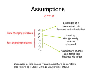
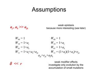
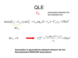
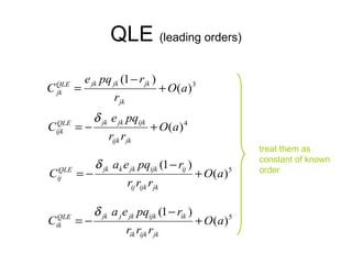
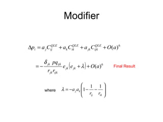
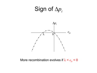
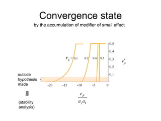
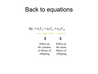
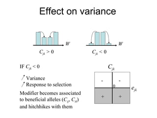
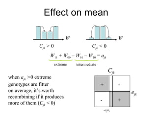
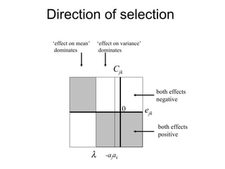
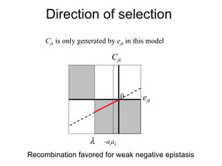
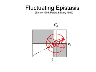
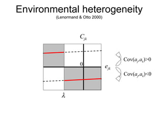
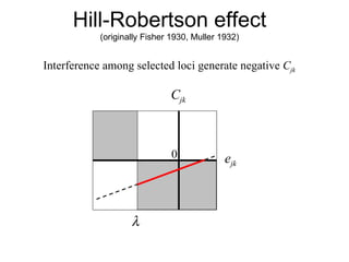
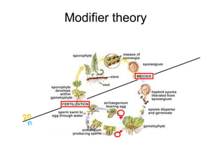
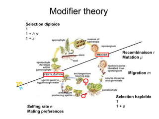
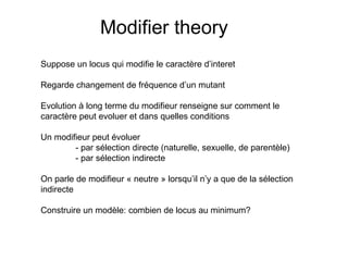
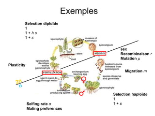
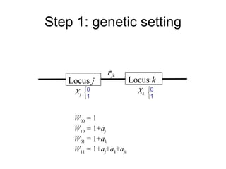
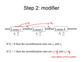
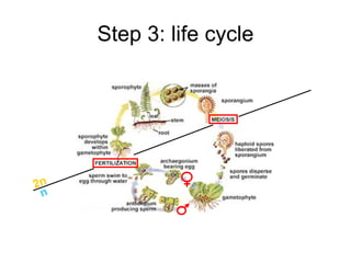
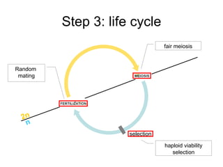
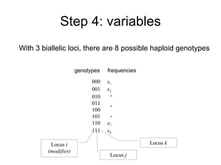
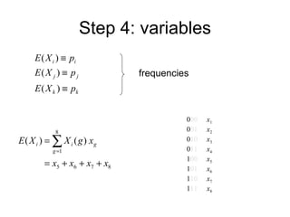
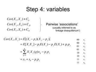
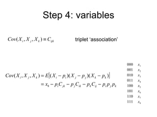
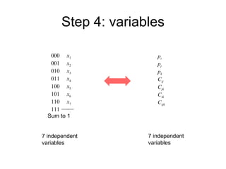
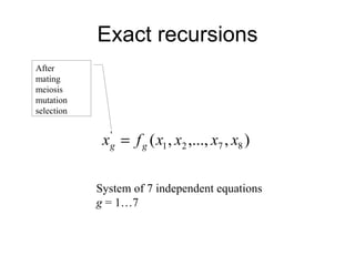
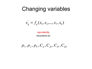
Population genetics Thomas Lenormand CEFE – CNRS, Montpellier
The mathematics of frequency change An allele arise by mutation Its frequency change for several reasons Genome change ( = evolution occurs) Mendel + Darwin A ‘microscopic view’ founding other approaches
G  P  P  G
(1892-1964) (1911-1998) (1890-1962) (1889-1988) (1920-2004) (1924-1994) (1916-  ) (1929 - )
Levins 1966 Généralité Précision Réalisme Un corpus de modèles Theories  - sexe - speciation - mort - altruisme Des  Stats… bcp de    stats - Mutations - Enzymes - Microsat - Sequences - Genomes
Réalisme distance  x 0 1 0 2 0 4 0 6 0 {R} {E} fréquence
Précison Saccheri I J et al. PNAS 2008;105:16212-16217 1/(4π D e σ 2 )
Généralité Probabilité de fixation Haldane 1927 … … 0 1 2 3 4 5 … 0 1 2 3 4 5 … P (1+ s ) P (1) P: proba fixation 1-P: proba perte X t  : nb de copies à la génération t P  ≈ 2 s
Modifier theory 2n n
Selection diploïde 1 1 +  h s 1 +  s Selection haploïde 1 1 +  s Recombinaison   r Mutation    Selfing rate    Mating preferences Modifier theory Migration  m 2n n
Modifier theory Suppose un locus qui modifie le caractère d’interet Regarde changement de fréquence d’un mutant Evolution à long terme du modifieur renseigne sur comment le  caractère peut evoluer et dans quelles conditions Un modifieur peut évoluer - par sélection directe (naturelle, sexuelle, de parentèle) - par sélection indirecte On parle de modifieur « neutre » lorsqu’il n’y a que de la sélection  indirecte Construire un modèle: combien de locus au minimum?
Selection diploïde 1 1 +  h s 1 +  s Selection haploïde 1 1 +  s sex Recombinaison   r Mutation    Selfing rate    Mating preferences Exemples Migration  m Plasticity 2n n
Reduction principle If viability loci at stable polymorphic equilibrium Transmission evolves to be « perfect » ( r  = 0,    = 0,  m  = 0,  sex  = 0) Selected loci are at equilibrium.  Selection coefficients are constant.  There is random mating.  Only one transmission parameter is considered at a time.  Viability is sex-independent.  (Altenberg and Feldman 1987)
Modifier vs. optimality Does modifier evolve to maximise mean fitness ? Knowing what would be best for the pop does not say that evolution  will lead there Modifiers are tools for modelling ‘ True’ genes have *always* pleiotropic effects
What is sex? 2n n
Why sex? What is the benefit of recombination? How to construct a model to measure this? Main hypothesis: sex allows for recombination
Part I Building the model from scratch Barton, N. H. 1995. A general model for the evolution of recombination.    Genetical Research 65:123-144.
Key insights Recombination   > 1 locus polymorphic   otherwise uninteresting Simplest polymorphism mutation – haploid selection Keep it simple single population very large number of individuals (neglect drift)
Step 1: genetic setting Locus  k Locus  j r jk W 00  = 1 W 10  = 1+ a j W 01  = 1+ a k W 11  =  1+ a j + a k + a jk X j X k 0 1 0 1
Step 2: modifier Locus  k Locus  j r jk X j X k Locus  i r ij X i If  X i  = 0 then the recombination rates are  r ij  and  r jk If  X i   = 1 then the recombination rates are  r ij +  ij  and  r jk +  jk Only effects of the modifier +  ij +  jk 0 1 0 1 0 1
Step 3: life cycle 2n n
Step 3: life cycle selection haploid viability selection fair meiosis Random  mating 2n n
Step 4: variables With 3 biallelic loci, there are 8 possible haploid genotypes 000  x 1 001  x 2 010 011 100 101 110  x 7 111  x 8 . .. genotypes frequencies Locus  i (modifier) Locus  j Locus  k
Step 4: variables frequencies 0 00   x 1  0 01   x 2 0 10   x 3 0 11   x 4 1 00   x 5 1 01   x 6 1 10   x 7 1 11   x 8
Step 4: variables frequencies 0 0 0   x 1  0 0 1   x 2 0 1 0   x 3 0 1 1   x 4 1 0 0   x 5 1 0 1   x 6 1 1 0   x 7 1 1 1   x 8
Step 4: variables Pairwise ‘associations’ 00 0   x 1  00 1   x 2 01 0   x 3 01 1   x 4 10 0   x 5 10 1   x 6 11 0   x 7 11 1   x 8 (usually referred to as    ‘linkage disequilibrium’)
Step 4: variables triplet ‘association’ 000  x 1  001  x 2 010  x 3 011  x 4 100  x 5 101  x 6 110  x 7 111  x 8
Step 4: variables 000  x 1  001  x 2 010  x 3 011  x 4 100  x 5 101  x 6 110  x 7 111  x 8 Sum to 1 7 independent  variables p i p j p k C ij C jk C ik C ijk 7 independent  variables
Part II Writing the equations
Exact recursions Aim :  computing variations of variables   over one generation 2n n selection (a) (b) (c)
Step 1: selection
Step 2: Fertilization  (random mating) Male gametes female gametes 000 001 010 011 100 101 110 111 000 x 1 2 001 x 1   x 2 x 2 2 010 x 1   x 3 x 2   x 3 x 3 2 011 … … … … 100 … … … … … 101 … … … … … … 110 … … … … … … … 111 … … … … … … x 7   x 8 x 8 2
Step 3: Meiosis Male gametes female gametes 001 010 001 010 000 011 (1- r jk )/2 (1- r jk )/2 r jk /2 r jk /2 Diploid individual produces gametes 000 001 010 011 100 101 110 111 000 x 1 2 001 x 1   x 2 x 2 2 010 x 1   x 3 x 2   x 3 x 3 2 011 … … … … 100 … … … … … 101 … … … … … … 110 … … … … … … … 111 … … … … … … x 7   x 8 x 8 2
Step 3: Meiosis Male gametes female gametes 101 110 001 010 000 011 (1- r jk -  )/2 (1- r jk -  )/2 ( r jk +  ) /2 Diploid individual produces gametes ( r jk +  ) /2 000 001 010 011 100 101 110 111 000 x 1 2 001 x 1   x 2 x 2 2 010 x 1   x 3 x 2   x 3 x 3 2 011 … … … … 100 … … … … … 101 … … … … … … 110 … … … … … … … 111 … … … … … … x 7   x 8 x 8 2
Exact recursions After mating meiosis mutation selection System of 7 independent equations g  = 1…7
Changing variables equivalently recursions on
Part III Analyzing the model
Methods When does the allele at the modifier locus change in frequency? The exact recursions give the answer, but they are not helpful Dynamical system: equilibria? Analysis involve assumptions Method 1 : stability analysis Method 2 : separation of time scales
Taylor Series constant approximation linear approximation quadratic approximation Notation :  Series[ f ( x ),{ x ,  x 0 , 2}] (like in Mathematica)
Assumptions r  >>  a p i  changes at a  even slower rate because indirect selection  Associations change  at a faster rate because  r  is larger p i p j p k C ij C jk C ik C ijk fast changing variables slow changing variables Separation of time scales = treat associations as constants also known as « Quasi Linkage Equilibrium » (QLE) p j  and  p k   change slowly because  a  is small
Assumptions a j  , a k  >>  a jk weak epistasis because more interesting (see later) W 00  = 1 W 10  = 1+ a j W 01  = 1+ a k W 11  =  1+ a j + a k + a jk W 00  = 1 W 10  = 1+ a j W 01  = 1+ a k W 11  = ( 1+ a j )(1+ a k )+ e jk a jk =e jk +a j a k    <<  r weak modifier effects investigate only evolution by the accumulation of small mutations
QLE C jk (association between the two selected loci) Association is generated by epistasis between the loci Recombination REDUCES associations
QLE  (leading orders) treat them as  constant of known order
Modifier where Final Result
Sign of   p i e jk  p i 0  More recombination evolves if    <  e jk  < 0
Convergence state -20 -15 -10 -5 0.1 0.2 0.3 0.4 0.5 r ij  =  0.1 0.2 0.5 0.4 0 by the accumulation of modifier of small effect (stability analysis) outside hypothesis made
Part IV Interpreting the model
Back to equations Effect on  the mean  fitness of  offspring Effect on the variance in fitness of offspring
Effect on variance Variance Response to selection + + - - Modifier becomes associated  to beneficial alleles ( C ij ,  C ik ) and hitchhikes with them IF  C jk  < 0 W C jk  >  0 W C jk  <  0 e jk C jk 0
Effect on mean W 11  +  W 00  –  W 01  –  W 10  =  a jk when  a jk  > 0 extreme  genotypes are fitter  on average, it’s worth recombining if it produces more of them ( C jk  < 0)  e jk C jk -a j a k + + - - extreme intermediate W C jk  >  0 W C jk  <  0
Direction of selection e jk -a j a k C jk  0 both effects positive ‘ effect on mean’  dominates both effects negative ‘ effect on variance’  dominates
Direction of selection e jk -a j a k C jk  0 C jk  is only generated by  e jk  in this model Recombination favored for weak negative epistasis
Part V Relate to other models
Fluctuating Epistasis  (Barton 1995, Peters & Lively 1999) e jk C jk  0
Environmental heterogeneity (Lenormand & Otto 2000) e jk C jk  0 Cov( a j ,a k )>0 Cov( a j ,a k )<0
Hill-Robertson effect (originally Fisher 1930, Muller 1932) e jk C jk  0 Interference among selected loci generate negative  C jk
Take home messages Recombination… is neutral in absence of associations can increase or decrease variance may increase variation but variation needs not be favourable can change both mean and variance in fitness frequency change depends on both the sign of genes associations and epistasis
Further? When to include stochasticity? Extending modifier theory to genome… Relationship to other approaches

Thomas Lenormand - Génétique des populations

  • 1.
    Population genetics ThomasLenormand CEFE – CNRS, Montpellier
  • 2.
    The mathematics offrequency change An allele arise by mutation Its frequency change for several reasons Genome change ( = evolution occurs) Mendel + Darwin A ‘microscopic view’ founding other approaches
  • 3.
    G P P G
  • 4.
    (1892-1964) (1911-1998) (1890-1962)(1889-1988) (1920-2004) (1924-1994) (1916- ) (1929 - )
  • 5.
    Levins 1966 GénéralitéPrécision Réalisme Un corpus de modèles Theories - sexe - speciation - mort - altruisme Des Stats… bcp de stats - Mutations - Enzymes - Microsat - Sequences - Genomes
  • 6.
    Réalisme distance x 0 1 0 2 0 4 0 6 0 {R} {E} fréquence
  • 7.
    Précison Saccheri IJ et al. PNAS 2008;105:16212-16217 1/(4π D e σ 2 )
  • 8.
    Généralité Probabilité defixation Haldane 1927 … … 0 1 2 3 4 5 … 0 1 2 3 4 5 … P (1+ s ) P (1) P: proba fixation 1-P: proba perte X t : nb de copies à la génération t P ≈ 2 s
  • 9.
  • 10.
    Selection diploïde 11 + h s 1 + s Selection haploïde 1 1 + s Recombinaison r Mutation  Selfing rate  Mating preferences Modifier theory Migration m 2n n
  • 11.
    Modifier theory Supposeun locus qui modifie le caractère d’interet Regarde changement de fréquence d’un mutant Evolution à long terme du modifieur renseigne sur comment le caractère peut evoluer et dans quelles conditions Un modifieur peut évoluer - par sélection directe (naturelle, sexuelle, de parentèle) - par sélection indirecte On parle de modifieur « neutre » lorsqu’il n’y a que de la sélection indirecte Construire un modèle: combien de locus au minimum?
  • 12.
    Selection diploïde 11 + h s 1 + s Selection haploïde 1 1 + s sex Recombinaison r Mutation  Selfing rate  Mating preferences Exemples Migration m Plasticity 2n n
  • 13.
    Reduction principle Ifviability loci at stable polymorphic equilibrium Transmission evolves to be « perfect » ( r = 0,  = 0, m = 0, sex = 0) Selected loci are at equilibrium. Selection coefficients are constant. There is random mating. Only one transmission parameter is considered at a time. Viability is sex-independent. (Altenberg and Feldman 1987)
  • 14.
    Modifier vs. optimalityDoes modifier evolve to maximise mean fitness ? Knowing what would be best for the pop does not say that evolution will lead there Modifiers are tools for modelling ‘ True’ genes have *always* pleiotropic effects
  • 15.
  • 16.
    Why sex? Whatis the benefit of recombination? How to construct a model to measure this? Main hypothesis: sex allows for recombination
  • 17.
    Part I Buildingthe model from scratch Barton, N. H. 1995. A general model for the evolution of recombination. Genetical Research 65:123-144.
  • 18.
    Key insights Recombination > 1 locus polymorphic otherwise uninteresting Simplest polymorphism mutation – haploid selection Keep it simple single population very large number of individuals (neglect drift)
  • 19.
    Step 1: geneticsetting Locus k Locus j r jk W 00 = 1 W 10 = 1+ a j W 01 = 1+ a k W 11 = 1+ a j + a k + a jk X j X k 0 1 0 1
  • 20.
    Step 2: modifierLocus k Locus j r jk X j X k Locus i r ij X i If X i = 0 then the recombination rates are r ij and r jk If X i = 1 then the recombination rates are r ij +  ij and r jk +  jk Only effects of the modifier +  ij +  jk 0 1 0 1 0 1
  • 21.
    Step 3: lifecycle 2n n
  • 22.
    Step 3: lifecycle selection haploid viability selection fair meiosis Random mating 2n n
  • 23.
    Step 4: variablesWith 3 biallelic loci, there are 8 possible haploid genotypes 000 x 1 001 x 2 010 011 100 101 110 x 7 111 x 8 . .. genotypes frequencies Locus i (modifier) Locus j Locus k
  • 24.
    Step 4: variablesfrequencies 0 00 x 1 0 01 x 2 0 10 x 3 0 11 x 4 1 00 x 5 1 01 x 6 1 10 x 7 1 11 x 8
  • 25.
    Step 4: variablesfrequencies 0 0 0 x 1 0 0 1 x 2 0 1 0 x 3 0 1 1 x 4 1 0 0 x 5 1 0 1 x 6 1 1 0 x 7 1 1 1 x 8
  • 26.
    Step 4: variablesPairwise ‘associations’ 00 0 x 1 00 1 x 2 01 0 x 3 01 1 x 4 10 0 x 5 10 1 x 6 11 0 x 7 11 1 x 8 (usually referred to as ‘linkage disequilibrium’)
  • 27.
    Step 4: variablestriplet ‘association’ 000 x 1 001 x 2 010 x 3 011 x 4 100 x 5 101 x 6 110 x 7 111 x 8
  • 28.
    Step 4: variables000 x 1 001 x 2 010 x 3 011 x 4 100 x 5 101 x 6 110 x 7 111 x 8 Sum to 1 7 independent variables p i p j p k C ij C jk C ik C ijk 7 independent variables
  • 29.
    Part II Writingthe equations
  • 30.
    Exact recursions Aim: computing variations of variables over one generation 2n n selection (a) (b) (c)
  • 31.
  • 32.
    Step 2: Fertilization (random mating) Male gametes female gametes 000 001 010 011 100 101 110 111 000 x 1 2 001 x 1 x 2 x 2 2 010 x 1 x 3 x 2 x 3 x 3 2 011 … … … … 100 … … … … … 101 … … … … … … 110 … … … … … … … 111 … … … … … … x 7 x 8 x 8 2
  • 33.
    Step 3: MeiosisMale gametes female gametes 001 010 001 010 000 011 (1- r jk )/2 (1- r jk )/2 r jk /2 r jk /2 Diploid individual produces gametes 000 001 010 011 100 101 110 111 000 x 1 2 001 x 1 x 2 x 2 2 010 x 1 x 3 x 2 x 3 x 3 2 011 … … … … 100 … … … … … 101 … … … … … … 110 … … … … … … … 111 … … … … … … x 7 x 8 x 8 2
  • 34.
    Step 3: MeiosisMale gametes female gametes 101 110 001 010 000 011 (1- r jk -  )/2 (1- r jk -  )/2 ( r jk +  ) /2 Diploid individual produces gametes ( r jk +  ) /2 000 001 010 011 100 101 110 111 000 x 1 2 001 x 1 x 2 x 2 2 010 x 1 x 3 x 2 x 3 x 3 2 011 … … … … 100 … … … … … 101 … … … … … … 110 … … … … … … … 111 … … … … … … x 7 x 8 x 8 2
  • 35.
    Exact recursions Aftermating meiosis mutation selection System of 7 independent equations g = 1…7
  • 36.
  • 37.
  • 38.
    Methods When doesthe allele at the modifier locus change in frequency? The exact recursions give the answer, but they are not helpful Dynamical system: equilibria? Analysis involve assumptions Method 1 : stability analysis Method 2 : separation of time scales
  • 39.
    Taylor Series constantapproximation linear approximation quadratic approximation Notation : Series[ f ( x ),{ x , x 0 , 2}] (like in Mathematica)
  • 40.
    Assumptions r >> a p i changes at a even slower rate because indirect selection Associations change at a faster rate because r is larger p i p j p k C ij C jk C ik C ijk fast changing variables slow changing variables Separation of time scales = treat associations as constants also known as « Quasi Linkage Equilibrium » (QLE) p j and p k change slowly because a is small
  • 41.
    Assumptions a j , a k >> a jk weak epistasis because more interesting (see later) W 00 = 1 W 10 = 1+ a j W 01 = 1+ a k W 11 = 1+ a j + a k + a jk W 00 = 1 W 10 = 1+ a j W 01 = 1+ a k W 11 = ( 1+ a j )(1+ a k )+ e jk a jk =e jk +a j a k  << r weak modifier effects investigate only evolution by the accumulation of small mutations
  • 42.
    QLE C jk(association between the two selected loci) Association is generated by epistasis between the loci Recombination REDUCES associations
  • 43.
    QLE (leadingorders) treat them as constant of known order
  • 44.
  • 45.
    Sign of  p i e jk  p i 0  More recombination evolves if  < e jk < 0
  • 46.
    Convergence state -20-15 -10 -5 0.1 0.2 0.3 0.4 0.5 r ij = 0.1 0.2 0.5 0.4 0 by the accumulation of modifier of small effect (stability analysis) outside hypothesis made
  • 47.
  • 48.
    Back to equationsEffect on the mean fitness of offspring Effect on the variance in fitness of offspring
  • 49.
    Effect on varianceVariance Response to selection + + - - Modifier becomes associated to beneficial alleles ( C ij , C ik ) and hitchhikes with them IF C jk < 0 W C jk > 0 W C jk < 0 e jk C jk 0
  • 50.
    Effect on meanW 11 + W 00 – W 01 – W 10 = a jk when a jk > 0 extreme genotypes are fitter on average, it’s worth recombining if it produces more of them ( C jk < 0) e jk C jk -a j a k + + - - extreme intermediate W C jk > 0 W C jk < 0
  • 51.
    Direction of selectione jk -a j a k C jk  0 both effects positive ‘ effect on mean’ dominates both effects negative ‘ effect on variance’ dominates
  • 52.
    Direction of selectione jk -a j a k C jk  0 C jk is only generated by e jk in this model Recombination favored for weak negative epistasis
  • 53.
    Part V Relateto other models
  • 54.
    Fluctuating Epistasis (Barton 1995, Peters & Lively 1999) e jk C jk  0
  • 55.
    Environmental heterogeneity (Lenormand& Otto 2000) e jk C jk  0 Cov( a j ,a k )>0 Cov( a j ,a k )<0
  • 56.
    Hill-Robertson effect (originallyFisher 1930, Muller 1932) e jk C jk  0 Interference among selected loci generate negative C jk
  • 57.
    Take home messagesRecombination… is neutral in absence of associations can increase or decrease variance may increase variation but variation needs not be favourable can change both mean and variance in fitness frequency change depends on both the sign of genes associations and epistasis
  • 58.
    Further? When toinclude stochasticity? Extending modifier theory to genome… Relationship to other approaches