Lecture-5 Types of iiiiii attributes.ppt

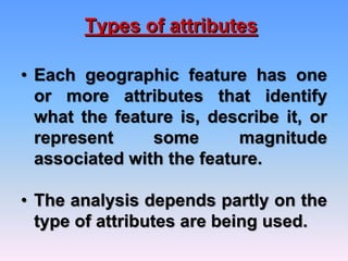
1. Types of attributes
• Each geographic feature has one
or more attributes that identify
what the feature is, describe it, or
represent some magnitude
associated with the feature.
• The analysis depends partly on the
type of attributes are being used.

2. Six kinds of basic attributes data are
used in GIS:
1. Nominal / Categories
2. Ordinal / Ranks
3. Interval
4. Ratio
5. Cyclic
6. Counts and amounts

3. Nominal / Categories
The simplest type of attribute, described by
name and to identify or distinguish one entity
from another, with no specific order.
Examples:
Categories of landuse, forest
etc.
Place names
Names of houses
Numbers on a driver's
license

4. • Categories are groups of similar things.
• These help to organize and make sense of your data.
• All features with the same value for a category are
alike in some way, and different from features with
other values for that category.
Each serves only to identify the particular instance of a
class of entities from other members of the same class.
Nominal attributes include numbers, letters, and even
colors.
Even though a nominal attribute can be numeric it
makes no sense to apply arithmetic operations to it:
adding two nominal attributes, such as two drivers'
license numbers, creates nonsense.

5. Categories of buildings

6. Ordinal / Ranks
List of discrete classes but with an inherent or
natural order / sequence.
Examples:
Orders of streams (first order, second
order…)
Level of education (primary, secondary….)

7. Ranks put features in order, from high
to low.
Ranks are used when direct measures
are difficult or if the quantity
represents a combination of factors.
Since the ranks are relative, you only
know where a feature falls in the order
you don’t know how much higher or
lower a value is than another value.

8. One can rate its agricultural land by classes of
soil quality, with Class 1 being the best, Class 2
not so good, etc.
Adding or taking ratios of such numbers
makes little sense, since 2 is not twice as much
of anything as 1, but at least ordinal attributes
have inherent order.
Averaging makes no sense either, but the
median, or the value such that half of the
attributes are higher-ranked and half are lower-
ranked, is an effective substitute for the
average for ordinal data as it gives a useful
central value.

9. Ranks

10. Interval
Attributes have natural sequence but in addition,
the distance between values have meaning.
Example:
The scale of Celsius temperature is interval,
because it makes sense to say that 30 and 20
are as different as 20 and 10.

11. Ratio
Attributes have the same characteristics as
interval variables, but in addition, these have
zero or starting point.

12. Example:
Rainfall per month
Weight is ratio, because it makes sense to say
that a person of 100kg is twice as heavy as a
person of 50kg; but Celsius temperature is only
interval, because 20 is not twice as hot as 10
(and this argument applies to all scales that are
based on similarly arbitrary zero points,
including longitude).

13. Directional or cyclic
In GIS, it is sometimes necessary to deal with
data that can be directional or cyclic, including
flow direction on a map, or compass direction,
or longitude.
The special problem here is that the number
following 359 is 0. Averaging two directions such
as 359 and 1 yields 180 the average of two
directions close to North can appear to be South.
This is somewhat analogous to the famous Y2K
bug, which originated because the next year after
1999 was 2000, not 1900, a problem for early
systems that did not record the first two digits of
the year.

14. Another set of problems arise because
latitude and longitude are often written in the
form of degrees, minutes, and seconds
(DMS), and computers are not normally able
to deal with the fact that adding one minute
to a latitude of 30 degrees, 59 minutes
produces 31 degrees and no minutes, not 30
degrees and 60 minutes.
The normal way of dealing with this problem
in GIS is to express latitude and longitude in
decimal degrees, not DMS, so 30 degrees 59
minutes would normally be stored as
30.98333... (Lee and Wong, 2001).

15. Examples:
In Arc View data measured at ratio or interval
scales are the type number, while data
measured at ordinal or nominal scales are
the type string.
There are Arc View functions such as
AsString or AsNumber that can be used to
convert attribute data between numerical
and string forms.

16. Counts and amounts
Counts and amounts show total numbers.
A count is the actual number of features on the
map.
An amount can be any measurable quantity
associated with a feature, e.g. no. of students
in a class.
Using a count or amount lets you see the
actual value of each feature as well as its
magnitude compared to other features.

17. Counts