Thermal properties

1. Lecture 3
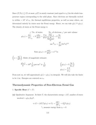
Fermi-Dirac Distribution at Finite Temperature
Accepting well-known results of statistical mechanics, we know that the number of elec-
trons in a given state at finite T is
nn =
1
eβ(n−µ) + 1
= f(n) β ≡
1
kT
This, of course, is the Fermi-Dirac distribution. The chemical potential
µ =
∂E
∂N
S
=
∂F
∂N
T
µ
n(E)
E
T 0
T = 0
Fermi Distribution Function
The Fermi distribution is symmetric about µ. This is particle-hole symmetry which
means that the distribution of particles is the same as the distribution of holes. Note
that at n = µ, the occupation f(n = µ) = 1/2. The smearing of the distribution ∼ kT.
At T = 0, distribution has an infinitely sharp-edge with µ(0) = F .
What happens to µ at finite T? If the metal is isolated, µ must be fixed implicitly
from the condition
N =
X
k,σ
fkσ(µ, T) =
X
k,σ
1
e(k−µ)/kT + 1
(N = number of conduction electrons available.)
Converting the sum to an integral gives
N =
∞
Z
0
df()g()
3.1

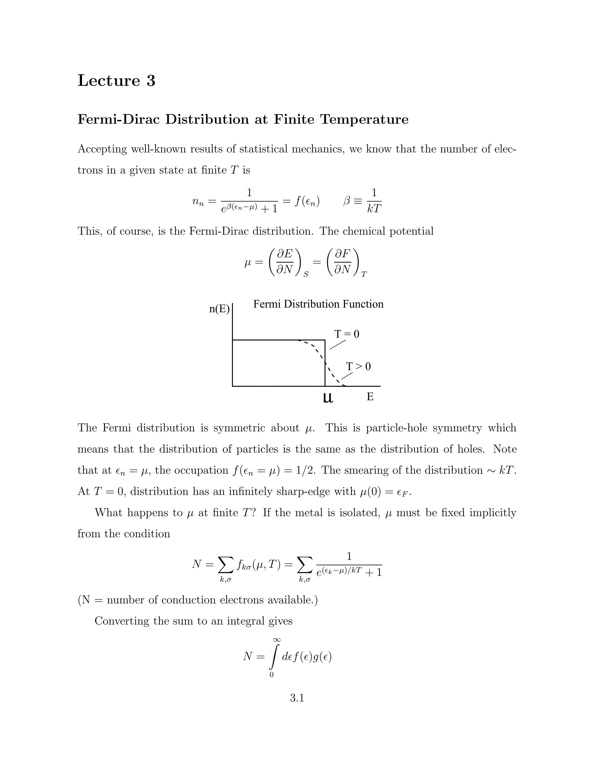
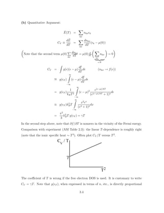
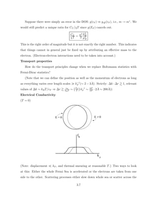
2. What happens to µ when T increases? The Fermi function f() is symmetric around
= µ, but g(), the density of states, is not - there are more states available at higher
energies.
µ
ε
g( )
ε ε
f( )g( ) .
To keep the integral of f()g() equal to N, f() must decrease ⇒ µ moves down
slightly as T increases. How much does µ decrease? A formal analysis is given in AM,
pp. 45-57, and Appendix C. The informal argument goes as follows: If the density of
states (DOS) g() were constant, µ would stay exactly at F for all T. At finite T, the
average excitation is ∼ kT above F , and so the average increase in the contribution of
the density of states is
δg() ∼ kT
dg()
d F
∼
kT
F
g(F ) (g() ∼
1
2 )
Thus the total increase in
R
d g()f() that would occur if µ = F is
∼ kT
kT
F
g(F ).
To compensate for this increase, we have to shift µ down by an amount proportional to
this. Since [µ] = energy, we expect
∆µ ∼ −kT
kT
F
∼ −
kT
F
2
µ(0)
(using µ(0) = F ). The precise answer is
µ(T) = µ(0) −
π2
12
T
TF
2
µ(0)
3.2

3. Since (T/TF ) . 1% at most, µ(T) is nearly constant (and equal to F ) for the whole tem-
perature region corresponding to the solid phase. Since electrons are thermally excited
to within ∼ kT of F , the thermal equilibrium properties, as well as some others, are
determined entirely by states near the Fermi energy. Hence, we can take g() ∼
= g(F ).
The density of states at the Fermi energy is
. No. of states No. of electrons . per unit volume
g(F ) =
dn
d F
= V
mkF
~2π2
=
V m
~2π2
r
2m
~2
1
2
F
| {z }
kF
= V
3n
2F
use ⇑F =
~2
2m
(3π2
n)2/3
Note g(F ) = V
mkF
~2π2
∼ n1/3
m
n =
k3
F
3π2
. Order of magnitude estimate:
g(F )
V
∼ 1023 1
eV
per cm3
1
kT
g(F ) = V
3n
2F
g(F ) =
3
2
N
F
From now on, we will approximate g() ∼ g(F ) in integrals. We will also take the limits
to be ±∞. Energies are centered on F .
Thermodynamic Properties of Free-Electron Fermi Gas
1. Specific Heat (C ∼ T)
(a) Qualitative Argument: At finite T, the characteristic energy ∼ kT, number of states
involved ∼ g(F )kBT,
⇒ E ∼ (kT)2
g(F ) ⇒ CV =
∂E
∂T v
∼ k2
BT g(f )
- measure energy from F = 0
3.3

4. (b) Quantitative Argument:
Ē(T) =
X
kσ
nkσk
CV ≡
dĒ
dT
=
X
kσ
dnkσ
dT
(k − µ(0))
Note that the second term µ(0)
P
kσ
dnkσ
dT
= µ(0) d
dT
X
kσ
nkσ
| {z }
=N
= 0
CV =
Z
g()( − µ)
df
dT
d (nkσ → f())
∼
= g(F )
∞
Z
−∞
( − µ)
df
dT
d
= g(F )
1
kBT2
∞
Z
−∞
( − µ)2 e(−µ)/kT
(e(−µ)/kT + 1)2
d
≡ g(F )k2
BT
∞
Z
−∞
x2
ex
(e2 + 1)2
dx
=
π2
3
k2
BT g(F ) = γT
In the second step above, note that ∂f/∂T is nonzero in the vicinity of the Fermi energy.
Comparison with experiment (AM Table 2.3): the linear T-dependence is roughly right
(note that the ionic specific heat ∼ T 3
). Often plot CV /T versus T2
.
V
C / T
T
γ
2
The coefficient of T is wrong if the free electron DOS is used. It is customary to write
CV = γT. Note that g(F ), when expressed in terms of n, etc., is directly proportional
3.4

5. to m
g(F ) =
V mkF
~2π2
=
V m(3π2
n)1/3
~2π2
⇒ γ ∝ geff (F ) ∝ m∗
Thus the fact that γ is not the free electron value γ0 can be described by saying that the
electron has an effective mass m∗
that gives it a different DOS. We can define
geff (F ) ≡
Cexp
v
π2
3
k2
BT
and
m∗
m
=
geff (F )
g(F )
=
γ
γ0
(It turns out that there are lots of different ways to define the effective mass and they
tend to give somewhat different numbers. What we have in the case of the specific heat
is the thermal effective mass.) Typically, m∗
∼ few · m. But heavy fermion systems
have m∗
/m ∼ 102
− 103
!
2. Pauli Paramagnetism (AM pp. 663-6)
What happens when we apply a magnetic field? The response of the electrons is re-
flected in the susceptibility: ~
M = χ ~
H. In the case of an electron gas, there are two con-
tributions to the susceptibility: Orbital diamagnetism and spin (Pauli paramagnetism).
These two effects can be separated in NMR. Here we will consider the paramagnetic
term.
The electron has a magnetic moment ~
µB directed along its spin which interacts with
~
H. The energy is ±µBH (the sign depends on the spin). Thus energy of up (down) spins
is shifted down (up) by µBH.
3.5

6. F
+
−
T = 0, H = 0
ε
ε
ε
g ( )
g ( )
ε
F
+
−
T = 0, H = 0
ε
ε
ε
g ( )
g ( )
ε
µΗ
µΗ
In equilibrium, spins will flow over from down to up to compensate, and the resulting
magnetization will be 2 × µB× (number flowing). The “2” comes because flipping a spin
from ↓ to ↑ changes its magnetization from +µB to −µB ⇒ δ ~
M = 2µB. The number
flowing = (number in the surplus region above F ) = 1
2
g(F )µBH since g(F ) is the density
of states for both spins. Hence
M = µ2
Bg(F )H
χ = µ2
Bg(F )
This should be approximately independent of T since the picture is the same at finite T.
Comparison with experiment (AM Table 31.5, p. 664): qualitative agreement but not
quantitative.
3.6

7. Suppose there were simply an error in the DOS: g(F ) ⇒ geff (F ), i.e., m → m∗
. We
would still predict a unique ratio for CV /χT since g(EF ) cancels out.
Cv
χT = π2
3
k2
B
µ2
B
This is the right order of magnitude but it is not exactly the right number. This indicates
that things cannot in general just be fixed up by attributing an effective mass to the
electron. (Electron-electron interactions need to be taken into account.)
Transport properties
How do the transport principles change when we replace Boltzmann statistics with
Fermi-Dirac statistics?
(Note that we can define the position as well as the momentum of electrons as long
as everything varies over length scales k−1
F (∼ 2 − 3Å). Strictly: ∆k · ∆r 1, relevant
values of ∆k ∼ kBT/vF ⇒ ∆r vF
kBT
∼ TF
T
k−1
F ∼ 104
102 · 2Å ∼ 200Å))
Electrical Conductivity
(T = 0)
E = 0 E = 0 .
fk
k
z
.
.
(Note: displacement kF , and thermal smearing at reasonable T.) Two ways to look
at this: Either the whole Fermi Sea is accelerated or the electrons are taken from one
side to the other. Scattering processes either slow down whole sea or scatter across the
3.7

8. Fermi surface. Energy conservation implies the latter is true ⇒ all the action goes on at
the Fermi surface.
The DC conductivity turns out to be the same as before.
Let’s calculate
dj
dt field
:
Rate of change of electric current = (e/m)× rate of change of total momentum
= (e/m)× total force = e
m
ne ~
E = ne2
m
~
E
⇒
d~

dt field
=
ne2
m
~
E as in Drude theory
Now calculate
dj
dt collision
. As before,
d~

dt collision
= −
~

τ
⇒
d~

dt total
=
d~

dt field
+
d~

dt coll
=
(
0 for DC
d
dt
(~
0eiωt
) for AC
⇒ σ(ω) =
σ0
1 − iωτ
where σ0 =
ne2
τ
m
Same as before. Hence all EM properties are identical in the two theories (including Hall
effect, etc.).
One difference: ` = vτ where v is “typical” velocity. In Drude theory v was the
classical thermal velocity vth ∼
p
kT/m. In Sommerfeld theory, v should be the Fermi
velocity: vF vth. Hence ` is much longer: at room temp. τ ∼ 10−14
sec, vF ∼ 108 cm
s
,
⇒ ` ∼ 10−6
cm ∼ 100Å.
Thermal Conductivity
Higher-energy particles tend to move in the positive direction, so the distribution is
distorted.
fk
k
z
.
.
Cold
Hot
3.8

9. Note: No net electron current in this approximation. h~
ji = −neh~
vi = 0 since h~
vi = 0.
Derivation of formula goes as before:
d~
Q
dt
diff
= −
1
3
v2CV ∇T
but v2 must now refer to the “active” electrons, so v2 = v2
F . Also
d~
Q
dt
coll
= −
~
Q
τ
as before
d~

dt tot
=
d~

dt diff
+
d~

dt coll
= 0
d~

dt diff
= −
d~
j
dt coll
~
jQ = −κ∇T
κ =
1
3
CV v2τ =
1
3
CV v2
F τ
Wiedemann-Franz Law
Derivation proceeds as before up to
κ
σT
=
1
3
CV v2m
ne2T
But now mv2 = mv2
F = 2F and
CV =
π2
3
k2
BTg(F ) = π2
k2
BT
n
2F
g(F ) =
3n
2F
⇒ K
σT
= π2
3
k2
B
e2
Instead of 3
2
(kB
e
)2
K
σT
∼ 2.44 × 10−8 W − Ω
k2
which is in very good agreement with experiment for most regimes.
Thermopower:
Again, the derivation goes through as in the Drude model up to the point Q =
− 1
3e
CV
n . Now, however, CV = π2
3 k2
BTg(F ) = π2
2 kB(T/TF )n so Q = −π2
6
kB
e (T/TF ).
3.9

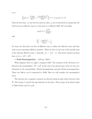
10. This is in much better agreement with experiment (but still not quantitatively right, and
can even have the wrong sign).
Electron-electron collisions - Effect on σ and κ
Any collision between electrons must conserve both energy and momentum (or ~
k):
1 + 2 = 0
1 + 0
2
~
p1 + ~
p2 = ~
p 0
1 + ~
p 0
2
Now the electrical current carried by a single electron is (−e)~
v = (−e/m)~
p. Hence
the total electrical current is unchanged by electron-electron collisions, so there is no
contribution to the relaxation rate τ−1
e` .
On the other hand, the heat current carried by an electron is (k −µ)~
v = (−µ)(~
p/m).
The sum of this quantity can be changed by collisions. Hence, it contributes to τ−1
Q .
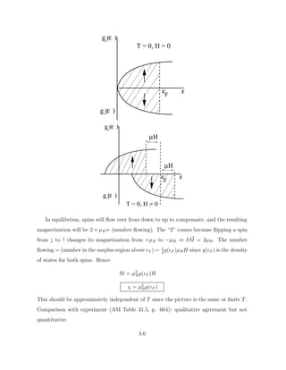
(Consider for example (1 = 2F , ~
p1 = pF x̂; 2 = 3F , ~
p2 = −pF x̂) → (0
1 = F , ~
p 0
1 =
−pF x̂; 0
2 = 4F , ~
p 0
2 = +pF x̂). Energy and momentum are conserved. But Σ( − µ)~
p/m
goes from −F
pF
m
x̂ to +3F
pF
m
x̂) (the product ( − µ) ~
p
m
is not conserved in collisions.)
Thus, if electron-electron collisions are important, we would expect W-F law to be
violated. Experimentally, however, it appears to hold very well (in most regimes). Why?
(answer below)
Effect of Exclusion Principle on Electron-Electron Collisions
For this purpose, we can forget all about the conservation of momentum and just
concentrate on the conservation of energy. According to Fermi’s Golden Rule, the scat-
tering probability ∝ (total) density of final states available. For example, consider a
“typical” electron with energy ( − µ) ∼ kT making a collision. It can collide with an
electron down to ∼ −kT of the Fermi surface (if below, no final states available): The
total “rearrangeable” energy in the collision is ∼ 2kT. Of the final energies, 0
1 and
0
2, one is fixed by energy conservation; the other is free and clearly ranges over ∼ kT
(F −kT . 0
. F +kT). Hence we have one factor of [kTg(F )] for the electron collided
with, and another for the final state. Thus, the collision prob. ∝ [kTg(F )]2
, or since
3.10

11. g(F ) ∼ T−1
F , τ−1
e`−e` ∼ (T/TF )2
τ−1
classical (relative to what it would be in a classical gas).
So, even if the mean free path ` in a classical gas was approximately the inter-electron
spacing (say ∼ 1Å), for any realistic degenerate system, it will be about 104
times this
(` ∼ 104
`classical ∼ 104
Å). Hence, electron-electron collisions are negligible compared to
other scattering mechanisms.
Successes and Failures of the Free Electron Model (after AM, Ch 3)
1. Static Thermodynamic Properties
Compressibility : Right order of magnitude but not quantitatively right
Specific Heat : the linear term seen experimentally and has right order of mag-
nitude, but model gives wrong quantitative value.
Pauli Paramagnetism : Temperature independence is as predicted, order of
magnitude right, quantitatively wrong. Cannot fix by simply introducing ef-
fective mass m∗
.
2. Transport Properties
• DC conductivity is plausible, but τ (or `) has to be put in by hand - difficult
to understand T-dependence within free electron model. Also resistivity ρ can
be anisotropic. Recall Matthiessen’s rule: τ−1
∼ τ−1
o + (τ−1
)0
T
• AC conductivity qualitatively right, but wrong ω-dependence in optical regime
• Wiedemann-Franz law: very well obeyed for T ∼ 300 K and T . few Kelvin;
otherwise it appears to fail (C ∼ T 3
due to phonons, κ due to phonons too)
• Hall coefficient - order of magnitude is right, but exact magnitude and some-
times even the sign is wrong
• Thermopower - ditto
• magnetoresistance - not in general zero as predicted by model (ρxx)
3.11

12. 3. Fundamental Difficulties
Why are some elements nonmetals? What determines the number of conduction
electrons? (It isn’t just the valence - consider, e.g., diamond and other forms of
carbon.)
We have made 3 major approximations:
(1) Free-electron approx. (ignore ions)
(2) Independent electron approx. (ignore electron-electron interactions)
(3) Relaxation-time approx. (ignore dependence of scattering process on history,
etc. of electrons)
Most of the difficulties are resolved if we keep (2) and (3) but relax (1). Thus we
must
(a) discuss ions as independent dynamic entities
(b) discuss effect of ions on electrons between collisions (periodic potential)
(c) discuss effect of ions on electrons as source of collisions (electron-phonon inter-
actions)
We now turn our discussion to (b). (a) and (c) come later.
3.12