Get 24/7 Reliable Chemical Engineering Assignment Help, Monatomic Ideal Gas Help, 100% error free, money back guarantee, Phd level tutors, A grade guarantee, www.HelpwithAssignment.com or email us at support@helpwithassignment.com

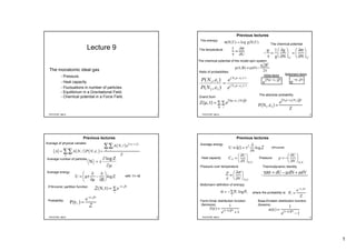
1. 1
PHY3TSP, 9&10 1
Lecture 9
The monatomic ideal gas
- Pressure.
- Heat capacity.
- Fluctuations in number of particles.
- Equilibrium in a Gravitational Field.
- Chemical potential in a Force Field.
PHY3TSP, 9&10 2
Previous lectures
The entropy:
The temperature
The chemical potential
The chemical potential of the model spin system.
τεμ
τεμ
ε
ε
/)(
/)(
22
11
22
11
),(
),(
−
−
= N
N
e
e
NP
NP
Ratio of probabilities:
Gibbs factor Boltzmann factor
Grand Sum
The absolute probability
PHY3TSP, 9&10 3
Previous lectures
Average of physical variable:
Average number of particles
μ
τ
∂
∂
=
Zlog
N
Average energy
with 1/τ =β
If N=const: partition function
Probability:
PHY3TSP, 9&10 4
Previous lectures
Average energy
(N=const)
Heat capacity Pressure
Pressure over temperature Thermodynamic Identity.
Boltzmann definition of entropy:
where the probability is:
Fermi-Dirac distribution function
(fermions)
Bose-Einstein distribution function
(bosons)

2. 2
PHY3TSP, 9&10 5
Previous lectures (8)
The energy of an electron in the orbital n (in 3D):
The density of states D:
Monatomic Ideal Gas: τετεμ
λε //)(
)( −−
=≅ eef
QcV=λ
τ
π
λ
τ
μ
mV
N 2
2
log
2
3
loglog +==
λ is the absolute activity
Number of particles:
The absolute activity:
γ is the number spin orientations
VQ is the quantum volume
The chemical potential:
The total energy:
τNU
2
3
=
The entropy:
c=N/V = concentration
PHY3TSP, 9&10 6
Pressure
σ V( ) = N logV + constan t
p
τ
=
∂σ
∂V
⎛
⎝
⎞
⎠ N,U
p
τ
=
N
V
Earlier we showed that the derivative of entropy with respect to volume gives
a relationship to pressure. Since entropy is essentially a logarithmic
expression we can write it as:
(9.1)
(9.2)
pV = Nτ
pV = NkBT
and
so
(9.3)
Thus,
The ideal gas law or equation of
state of an ideal gas.
MONOATOMIC IDEAL GAS (cont).
PHY3TSP, 9&10 7
One mole of gas contains N0 molecules, and for one mole:
TRTkNpV B == 0
117
0 degmolergs1031434.8 −−
×=≡ BkNR
23
0 1002217.6 ×=N
Where the gas constant R is:
N0 is the Avagadro number, defined as the number of molecules in one mole.
PHY3TSP, 9&10 8
CV = T
∂S
∂T
⎛
⎝
⎞
⎠V
= kBτ
∂σ
∂τ
⎛
⎝
⎞
⎠
CV ≡
∂U
∂T
⎛
⎝
⎞
⎠V
= kB
∂U
∂τ
⎛
⎝
⎞
⎠ V
U =
3
2
Nτ
CV =
3
2
NkB
The heat capacity at constant volume is defined as
The thermodynamic identity if dN=0 and dV=0
gives dU = T dS
Now for an ideal gas
so (9.6)
Heat Capacity.
(9.4)
(9.5)
1
2
kB CV =
3
2
Ror per degree of freedom. For one mole
.
τ = kBT and
S = kBσ

3. 3
PHY3TSP, 9&10 9
P
B
P
P k
T
S
TC ⎟⎟
⎠
⎞
⎜⎜
⎝
⎛
=⎟⎟
⎠
⎞
⎜⎜
⎝
⎛
=
τ∂
σ∂
τ
∂
∂
τdσ = dU − μdN + pdV
CP = T
∂S
∂T
⎛
⎝
⎞
⎠ P
=
∂U
∂T
⎛
⎝
⎞
⎠ P
+ p
∂V
∂T
⎛
⎝
⎞
⎠ P
The heat capacity at constant pressure is defined by
Using the thermodynamic identity (6.5) (N=const),
gives
When a gas is heated at constant pressure it expands against the
pressure and therefore does work. This means that to cause this effect
by heating will require more heat than at constant volume so the specific
heat will be larger.
(9.7)
(9.8)
What is the difference between CP and CV?
PHY3TSP, 9&10 10
internal2
3
internalnaltranslatio
uNN
UUU
+=
+=
τ
CV =
∂U
∂T
⎛
⎝
⎞
⎠ V
=
3
2
NkB + NkB
∂uint ernal
∂T
∂U
∂T
⎛
⎝
⎞
⎠P
=
3
2
NkB + NkB
∂uint ernal
∂T
We consider a polyatomic ideal gas, it will have the same translational
energy relationship as for a monatomic ideal gas but it will have more
degrees of freedom such as rotation and vibration (grouped as ‘internal’).
Thus the total energy is given by
The heat capacity at constant volume is:
But, from 9.10:
which is identical with 9.11 at constant V. From the ideal gas law
pV = NkBT we get
(9.10)
(9.11)
where uinternal is the vibrational and rotational energy of one molecule
(generalization of 9.6)
PHY3TSP, 9&10 11
p
∂V
∂T
⎛
⎝
⎞
⎠ p
= NkB
CP = T
∂S
∂T
⎛
⎝
⎞
⎠ P
=
∂U
∂T
⎛
⎝
⎞
⎠ P
+ p
∂V
∂T
⎛
⎝
⎞
⎠ P
= CV + NkB
CP =
3
2
NkB + NkB =
5
2
NkB
(9.12)
Combining (9.11) and (9.12) into (9.8) gives
A monatomic gas has:
(9.13)
BVP NkCC +=
For one mole of gas:
CP - CV = R
PHY3TSP, 9&10 12
ΔN( )2
≡ N − N( )2
= N2
− 2 N N + N 2
= N2
− N
2
ΔN( )2
= τ
∂ N
∂μ
N = eμ τ V
VQ
⎛
⎝
⎜
⎞
⎠
⎟
We have shown that:
and
Then have shown that for an ideal gas:
(9.14)
An ideal gas is in diffusive contact with a reservoir. What is the mean
square deviation of N from the 〈N〉? (check if the total number of particles in
a system is well-defined.)
Fluctuations in the number of particles
∂μ
∂τ
a
Z
Z
N = and we can easily show that:
2
22
2
∂μ
∂τ Z
Z
N =

4. 4
PHY3TSP, 9&10 13
Rearranging gives
ΔN( )2
= N
ΔN( )2
N 2 =
1
N
Thus the fractional fluctuation is of the order of the square root of 1/N. If N is
very large, ~ 1022 then the fractional fluctuation in the number of particles is
~ 10-11.
This demonstrates the accuracy with which a system in diffusive contact
simulates a system with a fixed total number of particles.
(9.16)
ΔN( )2
= τ
∂ N
∂μ
= τ
∂
∂μ
eμ τ V
VQ
⎛
⎝
⎜
⎞
⎠
⎟
⎡
⎣
⎢
⎤
⎦
⎥
= eμ τ V
VQ
⎛
⎝
⎜
⎞
⎠
⎟ = N
(9.15)
Mean square deviation:
PHY3TSP, 9&10 14
Equilibrium in a Gravitational Field.
The atmosphere can be treated to a
first approximation as an ideal gas
in a gravitational field. What would
be the variation of pressure with
height?
We consider two containers of gas,
one at a height L above the other
but in thermal and diffusive contact
so τ1 = τ2 and μ1 = μ2.
If an orbital s in the lower container has
energy εs, the corresponding orbital in
the upper container has energy
εs + MLg, where g is the acceleration of
gravity.
PHY3TSP, 9&10 15
( )[ ]
∑∑ −
= τεμ NN
eZ 1
1
ε + NMgL
( )[ ] ( ) ( )[ ]
∑∑∑∑ −−−−
== τεμτεμ NMgLNNMgLNN
eeZ 22
2
The grand sum for the lower container is
The energy of the corresponding N particle state in the upper parcel of gas
will have energy so the grand sum becomes
(9.18)
μ1 = τlogc1VQ
μ2 − MgL = τlogc2VQ
Where there is μ1 in Z1 there will be μ2-MgL in Z2. For the lower parcel we have:
and using the modified chemical potential for parcel 2 we have:
(9.19)
(9.17)
where εl(N) is the energy of an N-particle state in the lower container.
where c is concentration
PHY3TSP, 9&10 16
μ1 = τlogc1VQ = τlogc2VQ + MgL = μ2
τ log
c1
c2
= MgL
c2 = c1e
−MgL τ
p2 = p1e−MgL τ
These chemical potentials must be equal in equilibrium as the two parcels
are in thermal and diffusive contact so
giving
and (9.21)
which is the dependence of the concentration on height. Since p is
proportional to the concentration c then:
which is called the barometric pressure equation. This applies to an
isothermal atmosphere of a single chemical species, which the Earth's
atmosphere is not so it should be deviate from this equation.
(9.20)

5. 5
PHY3TSP, 9&10 17
There is a characteristic height
given by τ/Mg over which distance
the pressure drops by e-1 = 0.37.
Consider an atmosphere
composed of nitrogen molecules
with a molecular weight M=28.
If the temperature is 290K, then
this height is 8.5 km.
For molecules of lower mass the
height will be much larger. Thus,
molecules such as H2 and He will
escape the atmosphere in the
course of time.
Graph: the line is calculated pressure
for N2 at 290K, the crosses – actual
measurements.
PHY3TSP, 9&10 18
QcVlogτμ =
μ = τ logcVQ + MgL
The chemical potential of an ideal gas is given by
for an ideal gas with zero spin. This result was calculated with zero as the
energy of the lowest orbital.
In a gravitational field the energy levels are modified by the gravitational
potential energy and the chemical potential becomes
which is now made up of a term depending on the log (fractional
concentration) + a term depending on the potential energy of a particle.
Chemical potential in a Force Field.
where c is concentration at L.
PHY3TSP, 9&10 19
( )rrr φτμ qVc Q += )(log)(
( ) ( )222111 )(log)(log rrrr φτφτ qVcqVc QQ +=+
If q is the charge of a particle then qφ(r) is the potential energy of the
particle and the chemical potential will be
This result can be generalized to a system of charged particles in an
electrostatic potential Φ(r).
But for a system in diffusive equilibrium the chemical potential is constant
and independent of r. Thus changes in the electrostatic potential from r1 to r2
must be compensated by changes in the particle concentration from r1 to r2.
( )
( )
( ) ( )[ ] τφφ 21
1
2 rr
r
r −
= q
e
c
cor
This is important in semiconductors in which the potentials vary and hence
the concentration of carriers will also vary.
Ratio of the
concentrations
depends on potential
difference
PHY3TSP, 9&10 20
Problem
a) Show that the average pressure in a system in thermal contact with a
heat reservoir is given by
where the sum is over all states of the system.
Solution

6. 6
PHY3TSP, 9&10 21
(b) Using the expression for energy of a particle in a box
show that for a gas of free particles that
Since the entropy and N are constant the occupancy of the levels does not
change and the total pressure will be the ensemble average given by
p = −
dε
dV
⎛
⎝
⎜ ⎞
⎠
⎟e
−ε τ
∑
Z
PHY3TSP, 9&10 22
(c) Show that for a gas of free nonrelativistic particles
where U is the thermal average energy of the system. This is true for all
particles with zero rest mass.
PHY3TSP, 9&10 23
Lecture 10
Applications of the Fermi-Dirac Distribution: Metals
and White Dwarfs
- Degenerate Fermi gas.
- Ground state of Fermi gas in one dimension.
- Ground state of Fermi gas in three dimensions.
- Density of orbitals of free particles.
- Heat Capacity of an Electron Gas.
- Fermi Gas in Metals.
- White Dwarf Stars.
PHY3TSP, 9&10 24
A degenerate Fermi gas consists of non-interacting or weakly interacting
fermions at low temperature, τ << εF.
The orbitals below the Fermi energy will be mostly occupied and the orbitals
with higher energy will be mostly unoccupied.
The limit for the classical gas is the non-degenerate limit, τ >> εF.
The most important applications of the theory of degenerate Fermi gases are
to conduction electrons in metals, to the interiors of white dwarf stars, to
liquid He3, and to nuclear matter.
FERMI SYSTEMS
Degenerate Fermi Gas.

7. 7
PHY3TSP, 9&10 25
N free electrons (fermions) are confined in one dimension to an infinite well
of width L.
What orbitals will be occupied in the ground state of the system (remember
the Pauli’s exclusion principle)?
The electron orbitals are of the form sin(nπx/L) with n being the quantum
number. For each quantum number n there are two orbitals, one with spin
along the +z axis (spin up) and a particle with spin along the –z axis (spin
down).
Thus, each energy level labelled by the quantum number n has two orbitals,
one with spin up and one with spin down.
If the system has 8 electrons, then in the ground state the orbitals with
n=1,2,3, and 4 are filled and the orbitals with higher n are empty.
Introduce nF as the quantum number of the topmost filled orbital in the
ground state of a system of N noninteracting electrons.
Ground sate of Fermi gas in one dimension.
PHY3TSP, 9&10 26
Figure:
(a) The orbital energies of
the orbitals n=1,2,…12 for an
electron confined to a line of
length L. Each level
corresponds to two orbitals,
one for spin up and one for
spin down.
(b) The ground state of a
system of 16 electrons. The
orbitals above the shaded
region are vacant in the
ground state.
PHY3TSP, 9&10 27
εF =
2
2m
πnF
L
⎛
⎝
⎞
⎠
2
N =
π
3
nF
3
nF
2
=
3N
π
⎛
⎝
⎞
⎠
2
3
εF =
2
2m
3π2
N
V
⎛
⎝
⎜
⎞
⎠
⎟
2
3
Consider the system in the cube with side L. The Fermi energy is the energy
of the uppermost filled orbital at τ = 0K. If the quantum number for this orbital
is n = nF then
and the total number of particles is from which
Equation 10.1 can then be written
(10.1)
(10.2)
(10.3)
Ground state for Fermi Gas in 3 dimensions.
(L3=V)
PHY3TSP, 9&10 28
U0 =
π3
10m L
⎛
⎝
⎞
⎠
2
nF
5
=
3 2
10m
πnF
L
⎛
⎝
⎞
⎠
2
N =
3
5
NεF
Integrating gives:
(10.5)
U0 = 2 εn
n ≤nF
∑ = π dn n
2
εn
0
nF
∫ =
π3
2m L
⎛
⎝
⎞
⎠
2
dn n
4
0
nF
∫ (10.4)
Here we used
in the conversion of the sum into integral over an octant of a spherical shell
and for the energy of orbital:
∑ ∫→
n
ndn 2
2 π
22
2
⎟
⎠
⎞
⎜
⎝
⎛
=
L
n
m
n
π
ε
The average kinetic energy in the ground state is U0/N per particle, this is 3/5
of the Fermi energy
The total energy of the system in the ground state:

8. 8
PHY3TSP, 9&10 29
U0 =
π3
10m L
⎛
⎝
⎞
⎠
2
nF
5
=
3 2
10m
πnF
L
⎛
⎝
⎞
⎠
2
N =
3
5
NεF
• The plot of the energy U0
as a function of volume of a
mole of electrons is shown
in the figure.
• As the volume decreases
the energy increases so
that the Fermi energy is a
repulsive term in the
binding energy of a metal.
PHY3TSP, 9&10 30
D n( ) =
1
2
γπn
2
The density of orbitals D(n) was found to be
so the number of particles in the range n to n+Δn is D(n)dn.
(10.6)
• It is often more convenient to express the number of orbitals in terms of
energy. Then we can calculate the thermal averages as integrals over the
orbital energy ε.
• To do this, we will use a function called the density of orbitals or states.
• The density of orbitals is defined as the number of orbitals per unit
energy range and is denoted by D(ε)
Density of orbitals of free particles.
Where γ is the
number of
independent
spin orientations
PHY3TSP, 9&10 31
Figure: The number of orbitals in the energy range Δε is equal to the
number of orbitals in the quantum number range Δn=(dn/dε)Δε.
This is true if energy is function only of n.
PHY3TSP, 9&10 32
( ) ( )
( ) ( )
ε
γπ
ε
ε
εε
d
dn
n
d
dn
nDD
dnnDdD
2
2
1
==
=
(10.7)
ε =
2
2m
πn
L
⎛
⎝
⎞
⎠
2
n =
2mεL2
2
π2
⎛
⎝
⎜
⎞
⎠
⎟
1
2
dn
dε
=
mL2
2 2
π2
ε
⎛
⎝
⎜
⎞
⎠
⎟
1
2
D ε( ) =
γV
4π2
2m
2
⎛
⎝
⎞
⎠
3
2
ε
1
2
Thus from (10.7)
This is the density of orbitals.
If ε to ε+dε corresponds to n to n+dn then we can define a density of
orbitals D(ε) such that the number of states (orbitals) with energy between
ε and ε+ dε is equal:
(10.9)
(10.8)

9. 9
PHY3TSP, 9&10 33
Figure: the Fermi-Dirac distribution function versus energy, for two
temperatures. The value of f(ε) gives the fraction of orbitals at a given
energy which are occupied when the system in in the thermal equilibrium.
PHY3TSP, 9&10 34
The Fermi-Dirac distribution function gives the occupation of an orbital of
energy ε so D(ε)f(ε) is the density of occupied orbitals.
Figure: Density of orbitals as a
function of energy, for a free
electron gas in 3D. The dashed
curve represents the density of
occupied orbitals. The shaded
area represents the occupied
orbitals at absolute zero.
PHY3TSP, 9&10 35
U = dε εD ε( )f ε( )
0
∞
∫
N = dε D ε( )
0
εF
∫ U = dε εD ε( )
0
εF
∫
The same argument when applied to energy gives the average energy
of occupied orbitals = average energy of the system.
In the ground state, all orbitals are filled up to the Fermi energy:
(10.12)
The total number of electrons N in the system is then given by
(10.10)∫
∞
=
0
)(f)(D εεεdN
(10.11)
PHY3TSP, 9&10 36
ΔU = dε ε D ε( )
0
∞
∫ f ε( )− dε εD ε( )
0
εF
∫
To calculate the heat capacity we require the energy as a function of
temperature.
If a metal with N electrons is heated from 0K to τ then the energy required
is ΔU=U(τ)-U(0) or:
3
2
NkBT
whereas for metals it is much less. It was the recognition that the Fermi-
Dirac distribution function applied to electrons in a metal which explained
this apparent discrepancy.
For an ideal monatomic gas the heat capacity is
(10.13)
Heat Capacity of an Electron Gas.
N = dε D ε( )f ε( )
0
∞
∫ = dε D ε( )
0
εF
∫
We need to use some tricks to determine this integral. The total number
of particles in the system is given by
(10.14)

10. 10
PHY3TSP, 9&10 37
Splitting the integral in 10.13 into two parts gives
ΔU = dε ε D ε( )εF
∞
⌠
⌡
⎮ f ε( )+ dε ε D ε( )0
εF
⌠
⌡
⎮ f ε( )− dε ε D ε( )0
εF
⌠
⌡
⎮
Multiplying 10.14 by εF and splitting the integral into two parts
0 = − dε εF D ε( )f ε( )
εF
∞
⌠
⌡
⎮ − dε εF D ε( )f ε( )
0
εF
⌠
⌡
⎮ + dε εF D ε( )
0
εF
⌠
⌡
⎮
Adding the two equations gives
ΔU = dε ε − εF
⎛
⎝
⎜
⎞
⎠
⎟ D ε( )εF
∞
⌠
⌡
⎮ f ε( )+ dε εF − ε⎛
⎝
⎜
⎞
⎠
⎟ 1− f ε( )⎡⎣ ⎤⎦ D ε( )0
εF
⌠
⌡
⎮
The first term is the energy required to take electrons from an orbital with
energy εF to an energy ε > εF while the second is the energy required to lift
the energy of electron from ε to εF. The term D(ε)f(ε)dε is the number of
electrons elevated to orbitals in the energy range dε at the energy ε, while
[1 – f(ε)] is the probability that an electron has been removed from an
orbital ε.
PHY3TSP, 9&10 38
Figure: Fermi-Dirac distribution function at various temperatures. The electron
concentration of the Fermi gas was taken such that εF/kB = 50000 K, characteristic
of the conduction electrons in a metal.
PHY3TSP, 9&10 39
The Fermi energy is regarded as constant for temperatures up to TF/10
which is ~ 5000K so dependence of μ on τ is disregarded.
Figure: The chemical potential μ versus temperature τ for a gas of
noninteracting fermions in 3D.
PHY3TSP, 9&10 40
Cel =
dU
dT
= dε ε − εF
⎛
⎝
⎜⎜
⎞
⎠
⎟⎟
df
dT
D ε( )
0
∞
⌠
⌡
Cel = D εF( ) dε ε − εF
⎛
⎝
⎜⎜
⎞
⎠
⎟⎟
df
dT0
∞
⌠
⌡
Now the heat capacity is obtained by differentiating the energy with respect
to T so only those terms with a temperature dependence are considered,
i.e. terms with f(ε):
For low temperature τ<< εF the variation in f(ε) is only near the Fermi energy
so the density of states can be regarded as a constant in the integral (at
Fermi energy).
(10.18)
(10.17)
ΔU = dε ε − εF
⎛
⎝
⎜
⎞
⎠
⎟ D ε( )0
∞
⌠
⌡
⎮ f ε( )+ dε εF − ε⎛
⎝
⎜
⎞
⎠
⎟ D ε( )0
εF
⌠
⌡
⎮

11. 11
PHY3TSP, 9&10 41
df
dT
=
ε − εF
kBT2
e ε−εF( ) kBT
e ε−εF( ) kBT
+1[ ]
2
x ≡ ε − εF( ) kBT
Cel = kB
2
TD εF( ) dxx2 ex
ex
+1( )2
−εF kBT
∞
⌠
⌡
⎮
dxx
2 ex
ex
+1( )2 =
π2
3
−∞
∞
⌠
⌡
⎮
Cel =
1
3
π2
D εF( )kB
2
T
The chemical potential μ is very close to the Fermi energy for low
temperatures so we can replace it in F-D function:
Setting and combining 10.18 and 10.19
This is the standard integral:
(10.19)
(10.20)
(10.21)
(10.22)
Heat capacity of
electron gas
PHY3TSP, 9&10 42
D εF( )=
3N
2εF
=
3N
2kBTF
Cel =
1
2
π2
NkB
kBT
εF
=
1
2
π2
NkB
T
TF
Today’s problem will show that the density of orbitals at the Fermi energy:
So
(10.23)
(10.24)
This means that the specific heat is less than the ideal gas by approximately
the ratio of T/TF since the ideal gas CV is 3/2NkB.
Where FBF Tk≡ε
TF is not the temperature of the Fermi gas, but only convenient reference point. For
T<< TF the gas is degenerate and for T >> TF gas in a classical regime.
PHY3TSP, 9&10 43
εF =
2
2m
3π2
N
V
⎛
⎝
⎜
⎞
⎠
⎟
2
3
If the conduction electrons in metals act as a free fermion gas, the Fermi
energy may be calculated in terms of the concentration (10.3):
The concentrations are given in
the table (next slide) and the
Fermi energies are plotted in the
figure.
The alkali metals and copper, silver and gold have one free electron, or
conduction electron, per atom. The concentration of electrons is therefore
is equal to the concentration of the atoms, which can be evaluated from the
density of the atomic weight.
Fermi Gas in Metals.
PHY3TSP, 9&10 44
stop

12. 12
PHY3TSP, 9&10 45
1
2
mvF
2
= εF
CV = γT + AT3
CV
T
= γ + AT
2
The Fermi temperatures are the order of 5000K so the approximation that
T/TF << 1 are well founded.
The Fermi velocity is derived from the expression
The heat capacity of many metals at constant volume is the sum of the
electronic term plus the contribution of the lattice vibrations (phonons).
Usually the plots are made of CV/T v’s T2 since
when the points should lie on a straight line.
(10.25)
(10.26)
(10.27)
FB TNk /2
2
1
πγ ≡where is the electronic term from (10.24). The
electronic term is linear in T and is dominant at sufficiently low temperatures.
PHY3TSP, 9&10 46
γ0 =
π2
NkB
2
2εF
=
3.538×10−4
εF
J mol−1
deg−2
The comparison between γ and the calculated γ0 for an electron gas (10.24) is
with εF in eV. There is a good agreement between calculated and observed
values for monovalent metals.
(10.28)
Figure: Experimental heat capacity values for potassium
PHY3TSP, 9&10 47
White dwarfs are stars whose density is extremely high. It is believed that
the matter in such stars is completely ionised and the electrons form a
degenerate electron gas. A companion to Sirius, known as Sirius B was
discovered in 1844 by Bessel. The mass was determined to be 1.96 x
1030 kg and the radius 1.9 x 107 m and the temperature and energy
emitted was determined from Black Body radiation (Lecture 12).
The density of the star is 0.69 x 108 kg/m3 compared with the sun whose
density is about 1000 kg/m3.
White Dwarf Stars.
PHY3TSP, 9&10 48
If we calculate the Fermi energy based on this density we obtain from (10.3)
εF =
2
2m
3π2
N
V
⎛
⎝
⎜
⎞
⎠
⎟
2
3
= 3 x 105 eV
which is about 105 higher than a metal. The Fermi temperature is ~ 3 ´
109 K while the temperature of the star interior is 107 K. This temperature
can sustain the thermonuclear reaction which powers the star.
An analysis of the nuclei suggests that the nuclei form a gas which is
nearly degenerate.

13. 13
PHY3TSP, 9&10 49
Consider a free electron gas having N electrons. Show that the density of
orbitals at the Fermi level eF is
D εF( )=
3N
2εF
HINT: Use 10.3,
Problem
εF =
2
2m
3π2
N
V
⎛
⎝
⎜
⎞
⎠
⎟
2
3