This document summarizes the system identification and control of a two-cart spring system. Various identification techniques were used, including theoretical modeling, non-parametric methods like impulse response and sine sweeps, and parametric ARX modeling with chirp and square wave inputs. An ARX model with 3 poles was selected based on the identification results. An LQR/LQG controller was then designed and tuned, achieving reasonable closed-loop performance for controlling the position of the second cart.

1. ECE147C/ME106A Midterm Report
Lars Brusletto and Joaquim Dias Garcia
May 18, 2015
Abstract
This document contains the description of the methodology used to identify and control
the two-cart with spring system. Various systems identification techniques were employed
culminating in the choice of a ARX model using sine sweep data. An LQR/LQG controller were
implemented and tuned to obtain a reasonable response.
Contents
1 Introduction 1
2 System identification 2
2.1 Theoretical model . . . . . . . . . . . . . . . . . . . . . . . . . . . . . . . . . . . 2
2.2 Non-parametric identification . . . . . . . . . . . . . . . . . . . . . . . . . . . . 3
2.3 Parametric identification . . . . . . . . . . . . . . . . . . . . . . . . . . . . . . . 4
2.4 Identification results . . . . . . . . . . . . . . . . . . . . . . . . . . . . . . . . . . 6
3 Controlling the system 6
3.1 Controller design . . . . . . . . . . . . . . . . . . . . . . . . . . . . . . . . . . . 7
3.2 Closed-loop performance . . . . . . . . . . . . . . . . . . . . . . . . . . . . . . . 8
4 Conclusion 10
5 Bibliography 10
1 Introduction
The goal of this document is to report the laboratory results for the Project #1 of the course
ECE147C/ME106A of UCSB held during the Spring of 2015.
The problem addressed is the so called: Two-cart with spring. In this problem, there are
two carts moving in a fixed axis and they are connect with a spring. The first cart has a motor
that is activated by an electric circuit that provides electric power to the motor, the second
cart, on the other hand, is totally passive. The objective is to control the position of the second
1

2. cart by controlling the input of the motor. The only sensor available is an encoder that provides
the position of the second cart.
In order to solve this problem, one first has to obtain a reasonable model of the system
using system identification and subsequently design a controller that satisfies a set of given
specifications.
As reference material we used the project tutorial [3], the Lecture notes of the course [1]
and the book Linear Systems Theory by J.P. Hespanha [2].
The remaining of this document is organized as follows: Section 2 is the devoted to the
System Identification. Subsection 2.1 describes the theoretical model of the system, Subsection
2.2 presents the two experimental non-parametric identification of the system, Subsection 2.3
presents three experimental parametric identifications of the system Subsection 2.4 concludes
the Identification by presenting the model used in the remaining sections. Section 3 discusses
the control of the system, in Subsection 3.1 the controller design is described and Subsection 3.2
presents the closed loop performance of the system. Finally Section 4 provides the conclusion
and outlines directions for further improvements.
2 System identification
In this Section, the theoretical model of the two-cart with spring will be presented and various
methodologies for system identification will be experimentally applied in order to obtain a model
of the system to be controlled culminating in a final model to be used for the control procedure.
2.1 Theoretical model
The system to be identified consists two carts connected by a spring, both moving in a single
axis. The first cart has a motor that can be activated by an electric circuit and the second cart
is totally passive. The goal is to control the position of the second cart by varying the voltage
applied to the motor. Now we present the model following the lines of the project tutorial, to
make this document more self contained.
This system can be simplified by two masses connected by an ideal spring, where a force
acts on the first mass, this simplification is depicted in the Figure 1 below.
Figure 1: Simplified model of two-cart with spring
From newton’s laws one obtains the motion equations:
m1 :x1 “ kpx2 ´ x1q ` F m2 :x2 “ kpx1 ´ x2q (1)
where x1 and x2 are the positions of the first and second masses in meters, m1 and m2 are the
values of the first and second masses in kilograms and k is the spring constant in newtons per
2

3. meter. The force F is applied by the motor of the firs cart and can be modeled as:
F “
KmKg
Rmr
ˆ
V ´
KmKg
r
9x1
˙
(2)
where Km, Kg, Rm and r are parameters of the motor. V is the voltage applied to the motor in
volts and this is the input of the system, i.e. u :“ V . The only measured output of the system,
as said before, is the position of the second cart, i.e. y :“ x2.
The Laplace transform of the combination of the equations yields to the following transfer
function:
Hpsq “
Y psq
Upsq
“
2.97 ˆ 61.2
s4 ` 13.24s3 ` 127.15s2 ` 810.37s
(3)
As it will be noted in the following sections, it is not the true transfer function of the system.
However this model give some insight about the system such as the number of poles that are
expected in a simple and reasonably accurate model, as well as the fact that the system has
an integrator.
Another fundamental insight is that the system has no modes faster than 100 rad/s ( 15.9Hz),
since the transfer function decays monotonically after the resonance frequency and its mag-
nitude is below -100dB at 100rad/s, therefore the sampling frequency of 1ms used during the
whole experiment is much more that time faster than the fastest mode of the system as required
in [1] pg. 66.
2.2 Non-parametric identification
Two methods were used in this section: the approximated impulse response and the sine-wave
testing.
The impulse response method consist of exciting the motor with a impulse with duration
of 100ms and amplitude 5V, which is small enough to be fed to the motor by the operational
amplifier, whose linear regime is between negative and positive six volts, and big enough to
move the cart 15cm. The impulse response is given in the Figure 2
0 0.5 1 1.5
−0.02
0
0.02
0.04
0.06
0.08
0.1
0.12
0.14
0.16
time(s)
position(m)
Impulse Response
Figure 2: Impulse response of the system
Since we know that the system has an integrator we differentiated the data, then we applied
the Fourier transform, performed a complex curve fitting with 3 poles, and finally added back
3

4. the integrator to obtain a bode plot. To add back the integrator one just have to multiply the
values of each frequency by 1
jw (or 1
jΩ´1 , in case of discrete time), where w is the frequency
where the value was evaluated.
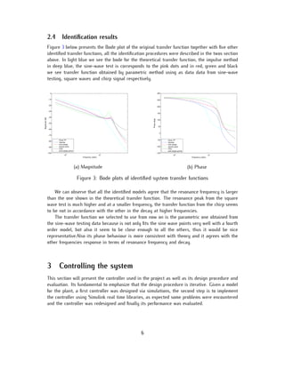
The bode plot of the impulse response is presented in the Figure 3 that also contains the
bode plot of the theoretical transfer function as well other bode plots whose evaluation will be
explained in the sequence.
Note that due to quantization, the differentiation procedure does not works well unless
some data processing is done. In this case we used a symmetric moving average with window
length 20. Note that the symmetric moving average as opposed to its causal counterpart does
not adds a phase delay in the data. It was also fundamental to test small variations in the
amplitude to make sure that the system was in the linear region, because if the input is too
small the measurement noise may be too big and if the input is too big the system may enter
in some non-linear regime.
The sine-wave testing consists of exciting the plant with different sine-waves one ant a time
and then evaluating the gain and phase shift for frequency. In this experiment we started by
choosing 20 different frequencies logarithmically spaced between 3 and 40 radians per second,
since that the region of the spectrum where we can see some interesting behaviour in the
theoretical plant. In order to model more precisely the plant in the resonance frequency we
did extra experiments with the frequencies 16.5, 18.5, 19.5, 21.2, 22.2, 24 and 25 radians per
second. For each frequency we recorded 30s of excitation. The magnitude of the sinusoids was
set at 4V for frequencies smaller than 10rad/s and 5V for the others, this was necessary to
make sure the carts were in linear region without hitting the wall.
Due to some non modelled dynamics sometimes the response to the sine-waves has some
linear trend that would make it impossible to use the correlation method as described in [1].
Besides that the results also have noise due to measurement and quantization. In order to solve
these problem we used the following signal processing technique: since the frequency of the
sine wave is known one can de-trend and smooth the series very efficiently by the least-squares
problem of minimizing the square errors eptq in: yptq “ β1 ` β2t ` β3cospwtq ` β4sinpwtq `
eptq, @t. The problem can be recast as:
minβ1,β2,β3,β4
ÿ
t
β1 ` β2t ` β3cospwtq ` β4sinpwtq ´ yptq (4)
Then the smoothed and de-trended output is given by: ˆyptq “
b
β2
3 ` β2
4sinpwt`atanpβ3{β4qq.
This data is then differenced, and the correlation method is applied to obtain a frequency re-
sponse, then the integrator is added to data and the results are presented in the figure 3.
2.3 Parametric identification
The parametric identification consists in using least-squares to obtain an ARX model, the details
are presented in [1]. In this project we used 3 kinds of inputs to obtain the model of the plant.
The first input is a Chirp signal with frequency varying from 3 to 80 rad/s during 100s, to
keep the process more robust to noise and in linear regime the amplitude was set to 4V, the
experiment was ran twice ans all the data was used.
The second kind of input is the square wave. We excited the plant with 4 different square
waves, each during 30 seconds their periods are: 1, 0.5, 0.25 and 0.2. All of them with amplitude
4

5. 3V to make measurements robust to noise and in the linear regime.
An easy method used here to verify if the system is in linear regime is simply to vary
slightly the amplitude and check whether the output varied linearly.
As in the impulse response method the data was smoothed using a symmetric moving
average, so that the quantization error is reduced. Also the data was differenced before the
ARX model was fitted, and the integrator was added back to the models by multiplying the
transfer functions by 1
z´1 .
As a third kind of input we used the smoothed and de-trended data from sine-testing of
subsection 2.2. The differencing was also used and the integrator was added back after the
transfer function was fitted.
With the three sets of data above we used Matlab command arx. From our prior knowledge
of the model we set the number of poles to be 3 (since the fourth is the integrator added after
the least-squares procedure). The number of zeros was varied from 0 to 3 in order to see which
gave better results in terms of SSE, conditioning of the matrix and transfer function plot, since
there is no direct connection between the number of zeros in continuous and discrete time, due
to different possible discretization schemes. The transfer functions obtained, respectively, from
the Chirp, Square waves and Sine-wave test inputs follow:
Hpzq “ 5.6 ¨ 10´5 pz ´ p1.0177 ` j0.0243qqpz ´ p1.0177 ´ j0.0243qq
pz ´ 1qpz ´ p0.9946 ` j0.0202qqpz ´ p0.9946 ´ j0.0202qqpz ´ p´0.3927qq
(5)
Hpzq “ 6.9 ¨ 10´7 pz ´ p1.6170qqpz ´ p1.0726qq
pz ´ 1qpz ´ p0.9988 ` j0.0183qqpz ´ p0.9988 ´ j0.0183qqpz ´ p´0.3152qq
(6)
Hpzq “ 3.3 ¨ 10´8 pz ´ p1.1577qqpz ´ p0.8986qq
pz ´ 1qpz ´ p0.9973 ` j0.0220qqpz ´ p0.9973 ´ j0.0220qqpz ´ p0.9936qq
(7)
The main statistics from the least squares procedures used are presented in the following
table:
SSE Max std.dev. of zeros Max std.dev. of poles
Chirp 5.5 ¨ 10´14 6.2 ¨ 10´6 6.0 ¨ 10´3
Square Wave 4.4 ¨ 10´14 1.8 ¨ 10´7 6.3 ¨ 10´3
Sine Wave Testing 8.1 ¨ 10´21 2.8 ¨ 10´7 5.9 ¨ 10´6
In the table one can observe that it does not seem to have problem with the SSE since
they are indeed very small, big values would be a problem. From the maximum values of the
standard deviation of the estimates of the zeros and the poles one can see that the the first
two models seem to be just reasonably well conditioned, whereas the third model seems to be
the one with best well conditioned matrix, for more information on these conditioning test see
[1] pg. 50 and 56.
Also the small standard deviation for the estimation in the sine’s model show that we can
have high confidence in its results.
5

6. 2.4 Identification results
Figure 3 below presents the Bode plot of the original transfer function together with five other
identified transfer functions, all the identification procedures were described in the twos section
above. In light blue we see the bode for the theoretical transfer function, the impulse method
in deep blue, the sine-wave test is corresponds to the pink dots and in red, green and black
we see transfer function obtained by parametric method using as data data from sine-wave
testing, square waves and chirp signal respectively.
10
0
10
1
−100
−90
−80
−70
−60
−50
−40
−30
−20
−10
0
Frequency (rad/s)
Magnitude(dB)
Given TF
Impulse
sine sweep
square wave
chirp
sine sweep points
(a) Magnitude
10
0
10
1
−150
−100
−50
0
50
100
150
200
250
300
Frequency (rad/s)
Phase(deg)
Given TF
Impulse
sine sweep
square wave
chirp
sine sweep points
(b) Phase
Figure 3: Bode plots of identified system transfer functions
We can observe that all the identified models agree that the resonance frequency is larger
than the one shown in the theoretical transfer function. The resonance peak from the square
wave test is much higher and at a smaller frequency, the transfer function from the chirp seems
to be not in accordance with the other in the decay at higher frequencies.
The transfer function we selected to use from now on is the parametric one obtained from
the sine-wave testing data because is not only fits the sine wave points very well with a fourth
order model, bot also it seem to be close enough to all the others, thus it would be nice
representative.Also its phase behaviour is more consistent with theory and it agrees with the
other frequencies response in terms of resonance frequency and decay.
3 Controlling the system
This section will present the controller used in the project as well as its design procedure and
evaluation. Its fundamental to emphasize that the design procedure is iterative. Given a model
for the plant, a first controller was designed via simulations, the second step is to implement
the controller using Simulink real time libraries, as expected some problems were encountered
and the controller was redesigned and finally its performance was evaluated.
6

7. 3.1 Controller design
We have chosen to implement a LQR/LQG controller because it is less dependent of heuristic
choices such as pole placement. Also, once one have a state space model that is sufficiently
accurate, it is very simple to implement and tune this kind of controller.
Since the transfer function obtained from the sine-wave testing seems to be the best of the
parametric models as stated in subsection 2.4 it was chosen to be used for the control design.
Given the discrete time transfer function, the first step to obtain the controller is to obtain
continuous time transfer function, this was done by using the Zero-Order-Hold approximation,
which is the default in matlab’s command d2c. The following step is to obtain a state space
model, this can be done using the command tf2ss, that realized the system in controllable
canonical form.
Using the notation of [2] pg.234, sections 23.6 and 23.7, for LQR/LQG, one has to choose
basically 2 tuning parameters: ρ which balances the penalization on the size of the steady
state error and the input; the second parameter is σ which represents the level of confidence
that the kalman filter should have in the measured data.
The first choice of ρ and σ were done in simulation outside the laboratory. However when
it was implemented in the laboratory the following problems were encountered: the input would
take a while to reach its maximum value, which means that the settling time was way to long
(around 1 second) and the steady state error was significantly big (around 8 percent). We
could observe that the steady state error was due to static friction because small inputs that
should correct this error were not enough to move the cart.
In order to try to improve the controller performance we first tried to connect in parallel with
the LQR/LQG, which is a proportional controller, an integrator to reduce the steady state error
and a differentiator to reduce the rise time, however we did not have significant improvement
in these characteristics. So we tried another procedure: we simulated outside the lab an
LQR/LQG taking into account an approximation for static friction by setting the input to zero
if its smaller that 0.5V, this yielded to a new choice of ρ and σ.
Back in the laboratory the controller performance was much better and the steady state
error was reduced to 1 percent, however the rise time was not fast enough. To overcome this
final problem we observer the states of the Kalman filter and noticed that one of them was
much more similar to position that the others, thus we increased the gain of that state by
20 percent which made the rise time much faster. The final choice of tuning parameters was:
ρ “ 0.00005, σ “ 0.00001 and the fourth entry of the gain matrix K was multiplied by 1.2.
Figure 4: Coupler Made of Microstrip
For better presentation the simulated step response and bode plots will be presented in
next section.
7

8. 3.2 Closed-loop performance
Given the final choice of controller its was implemented in the laboratory and its performance
was evaluated by observing the properties of the step response and a closed loop identification.
The closed loop identification was done by using the method of sine-wave testing. We used
32 frequencies between 0.3 and 40 radians per second, all the sine waves with amplitude 10cm
and the data was recorded during 30s. As in the sine wave-test of the open loop the series
were smoothed by the same procedure to obtain more accurate results. The resulting Bode
plot is given in Figure 5.
10
0
10
1
−50
−40
−30
−20
−10
0
10
Frequency (rad/s)
Magnitude(dB)
Simulated Closed Loop with Given TF
Simulated Closed Loop with TF from ID
Identified Closed Loop
(a) Magnitude
10
0
10
1
−400
−300
−200
−100
0
100
200
Frequency (rad/s)
Phase(deg)
Simulated Closed Loop with Given TF
Simulated Closed Loop with TF from ID
Identified Closed Loop
(b) Phase
Figure 5: Bode plot of the designed controller
In Figure 5 one can observe that there are significant differences between the three plots.
The deep blue line that represents the simulated closed loop responses always below zeros and
its almost constant zeros from DC up to around 10 rad/s, showing that in theory the controller
would be able to perform good tracking in such range, the phase plot shows typical behaviour of
a LQR/LQG controller. The light blue line represents the closed loop that arises from combining
the theoretical plant with the controller designed from the identified plant, the fact that the
bode plot is significantly different from the previous make sense since as we saw in Figure 3
the laboratory plant has a very different resonance frequency for all identified models, which
confirms that the theoretical model is actually a poor approximation in this case, indeed such
closed loop is even unstable!
Finally the pink dots correspond to the sine wave testing of the closed loop. One can note
significant differences from this last bode to the firs one. Firstly, for very low frequencies, below
3 rad/s the magnitude is around -1.3dB, instead of 0 and the phase is very delayed instead of
the expected zero delay, from our observation this behaviour seems to be due basically to static
friction because the tracking position varies very slowly so that the correspondent input mus
be very small which is usually not enough to overcome static friction. For frequencies between
3 and 8rad/s the controller seem to perform very good tracking since the magnitude bode is
basically zero, nevertheless the phase is 50 degrees more delayed than expect, this could be
due to a not fast enough settling time that will be commented hereafter. Around 11 rad/s the
closed loop seems to have a slight resonance frequency, since the phase starts to decay and
8

9. the magnitude is around 2dB (in the maximum). From 15 to 20 rad/s is actually the best range
of tracking, since the magnitude is basically zeros, also the phase is very close to the expected
from simulations. Lastly, fro frequencies higher than 20 rad/s the magnitude drops a lot since
the controller was designed from a model that would decay fast in this part of the spectrum,
interestingly the simulated closed loop seems to decay significantly only in higher frequencies,
this might be due to some unmodelled non-linearities.
Now we present the control performance in time domain. Figure 6 shows the step response
of the simulated close loop in blue and the experimental closed loop in red, some of the
characteristics of such curve are summarized in the table below. The smaller overshoot in the
experimental closed loop might be due to the effect of friction that is a non-linear effect that
was not modelled, this is probably also the reason for slower rise time in the experiment than
in the simulation. Interestingly the settling time was larger in the simulation, but this is due to
the smaller overshoot. Also we had a 1% steady state error, because the output of the controller
was too small to overcome static friction. The maximum control magnitude are very similar and
the smaller value for the experimental set-up is consistent with the smaller overshoot. Note
that the maximum control magnitude correspond to a step of 10cm, the steps in Figure 6 were
converted to unit size for simplicity.
0 0.2 0.4 0.6 0.8 1 1.2
0
0.5
1
1.5
From: In(1) To: y1
Closed Loop Step Response
Time (seconds)
Amplitude
Simulated
Experimental
(a) Step response
0 1 2 3 4 5 6
−0.04
−0.02
0
0.02
0.04
0.06
0.08
0.1
0.12
Step Response under Measurement error
time (s)
position(m)
10%
5%
1%
(b) Square wave response under measurement noise
Figure 6: Time domain performance analysis
Simulated Experimental
Rise-time 0.122s 0.155s
Overshoot 12.8% 7.3%
Settling time 0.472s 0.420s
Maximum control magnitude 5.8V 5.37V
Steady state error 0% 1%
In order to understand how robust the designed controller is we performed 3 simulation
tests. In these tests we added Gaussian random noise with standard deviation: 0.008 (10%
of step size), 0.004 (5% of step size) and 0.0008 (1% of step size). From the results presented
in Figure 6 we can observe that the steady state error were respectively 37%, 20% and 2%.
9

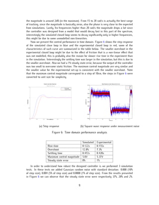
10. These results were reasonable because the variances of the noise used are much bigger than
actual measurement error in this experiment. An error of only 2% in the last case show that
the controller is reasonably robust.
4 Conclusion
In this project we were able to apply the theory of system identification and the LQR/LQG
controller design to obtain a reasonable controller for the twos cart with spring problem.
We were able to obtain a parametric model to the system that was show to be a fine
approximation and we could design a controller that had a good performance given all the
non-linearities and noise effects that were not modelled. The very small steady state error of
the controller to together with its small overshoot seem to be nice results.
If we had more time to work in such project we could try to combine integrator and
differentiators in a more systematic way so that the controller could benefit from it. Also
we could expend some time figuring out some more intuitive realization, so that we could
understand better the states and use this knowledge to improve the controller performance.
Another direction we could take is try to implement a H-infinity controller using the Glover-
mcFarlane procedure.
5 Bibliography
References used in this work:
[1]-J.P.Hespanha. Topics in undergraduate control systems. Availble at https://www.ece.
ucsb.edu/~hespanha/published, Apr 2006
[2]-J.P. Hespanha. Linear Systems Theory. Princeton Press, Sep. 2009. ISBN13: 978-0-
691-14021-6.
[3]-J.P. Hespanha. ECE147C/ME106A Poject #1: Two-cart with spring, Mar. 2014.
10