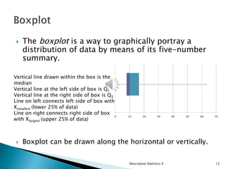
This document provides an overview of descriptive statistics, focusing on the concepts of data shape, skewness, and methods for calculating and visualizing these properties using tools like MS Excel. It details how to compute z-scores, create frequency distributions, and analyze graphical representations such as boxplots and histograms. Additionally, it discusses the importance of understanding data distribution, skewness, and relationship analysis through correlation and regression.

1. Part II
Each slide has its own narration in an audio file.
For the explanation of any slide click on the audio icon to start it.
Professor Friedman's Statistics Course by H & L Friedman is licensed under a
Creative Commons Attribution-NonCommercial-ShareAlike 3.0 Unported License.

2.  A third important property of data – after
location and dispersion - is its shape.
 Shape can be described by degree of
asymmetry (i.e., skewness).
◦ mean > median positive or right-skewness
◦ mean = median symmetric or zero-skewness
◦ mean < median negative or left-skewness
 Positive skewness can arise when the mean is
increased by some unusually high values.
 Negative skewness can arise when the mean is
decreased by some unusually low values.
Descriptive Statistics II 2

3.  Left skewed:
 Right skewed:
 Symmetric:
Descriptive Statistics II 3
Source: Levine et al., Business Statistics, Pearson, 2013.

4. Data (for n=12 employees):
2 3 8 ┋ 8 9 10 ┋ 10 12 15 ┋ 18 22 63
𝑋= 180/12 = 15 hours
Median = 10 hours
The (extremely slow) employee who took 63 hours to
complete the task skewed the entire distributon to the
right.
s2 = 2868 / 11 = 260.79
s = 16.25 hours
CV = 107.7%
Descriptive Statistics II 4
This guy
took a VERY
long time!

5.  Scores of 17 students on a national calculus
exam. Data:
0, 0, 10, 12, 15, 18, 20, 25, 30, 33, 34, 41, 56,
87, 92, 94, 95
 Open MS Excel.
 Go to Data Analysis—Analysis Tools —
Descriptive Statistics.
 If you do not have Data Analysis-Analysis Tools, you
have to use the Add-in feature and add it to MS Excel.
 Make sure to check the Summary Statistics box
once you are in descriptive statistics.
 See MS Excel Output on next slide.
Descriptive Statistics II 5

6. MS Excel uses a formula – the Pearson Coefficient of
Skewness – to calculate skewness. You do not have to know
the formula. If the coefficient is 0 or very close to it, you
have a symmetric distribution.
Descriptive Statistics II 6
Column1
Mean 38.94117647
Standard Error 8.111117365
Median 30
Mode 0
Standard Deviation 33.44299364
Sample Variance 1118.433824
Kurtosis -0.82259021
Skewness 0.782252352
Range 95
Minimum 0
Maximum 95
Sum 662
Count 17
From the output:
• mean is 38.94
• median is 30
• mode is 0
• standard deviation is 33.44
• variance is 1118.43
• skewness is .78 (positive)
• range is 95
• n is 17

7.  We can convert the original scores to new
scores with 𝑋 = 0 and s = 1.
 This will give us a pure number with no
units of measurement.
 Any score below the mean will now be
negative.
 Any score at the mean will be 0.
 Any score above the mean will be positive.
Descriptive Statistics II 7

8. To compute the Z-scores:
𝑍 =
𝑋 − 𝑋
𝑠
Example.
Data: 0, 2, 4, 6, 8, 10
𝑋 = 30/6 = 5; s = 3.74
Descriptive Statistics II 8
X  Z
0 0−5
3.74
-1.34
2 2−5
3.74
-.80
4 4−5
3.74
-.27
6 6−5
3.74
.27
8 8−5
3.74
.80
10 10−5
3.74
1.34

9. Descriptive Statistics II 9
 Data: Exam Scores
Original data Change 7 to 97 Change 23 to 93
X Z X Z X Z
65 -0.45 65 -0.81 65 -1.40
73 -0.11 73 -0.38 73 -0.79
78 0.10 78 -0.10 78 -0.40
69 -0.28 69 -0.60 69 -1.09
78 0.10 78 -0.10 78 -0.40
7 -2.89 <= 97 0.94 97 1.07
23 -2.21 23 -3.12 <= 93 0.76
98 0.94 98 0.99 98 1.14
99 0.99 99 1.05 99 1.22
99 0.99 99 1.05 99 1.22
97 0.90 97 0.94 97 1.07
99 0.99 99 1.05 99 1.22
75 -0.02 75 -0.27 75 -0.63
79 0.14 79 -0.05 79 -0.32
85 0.40 85 0.28 85 0.14
63 -0.53 63 -0.92 63 -1.56
67 -0.36 67 -0.70 67 -1.25
72 -0.15 72 -0.43 72 -0.86
73 -0.11 73 -0.38 73 -0.79
93 0.73 93 0.72 93 0.76
95 0.82 95 0.83 95 0.91
Mean 75.57 Mean 79.86 Mean 83.19
s 23.75 s 18.24 s. 12.96

10.  No matter what you are measuring, a Z-score of
more than +5 or less than – 5 would indicate a
very, very unusual score.
 For standardized data, if it is normally distributed,
95% of the data will be between ±2 standard
deviations about the mean.
 If the data follows a normal distribution,
◦ 95% of the data will be between -1.96 and +1.96.
◦ 99.7% of the data will fall between -3 and +3.
◦ 99.99% of the data will fall between -4 and +4.
 Worst case scenario: 75% of the data are between 2
standard deviations about the mean.
[Chebychev.]
Descriptive Statistics II 10

11.  When examining a distribution for shape,
sometime the five number summary is useful:
Smallest| Q1 | Median | Q3 | Largest
 Example:
𝑋 = 15
5-number summary: 2 | 8 | 10 | 16.5 | 63
This data is right-skewed.
In right-skewed distributions, the distance from Q3 to
Xlargest (16.5 to 63) is significantly greater than the distance
from Xsmallest to Q1(2 to 8).
Descriptive Statistics II 11
2 3 8 8 9 10 10 12 15 18 22 63
Smallest Largest
Median
Q1
Q3

12.  The boxplot is a way to graphically portray a
distribution of data by means of its five-number
summary.
 Boxplot can be drawn along the horizontal or vertically.
Descriptive Statistics II 12
Vertical line drawn within the box is the
median
Vertical line at the left side of box is Q1
Vertical line at the right side of box is Q3
Line on left connects left side of box with
Xsmallest (lower 25% of data)
Line on right connects right side of box
with Xlargest (upper 25% of data)

13.  A “bell-shaped” symmetric data distribution
would look like this:
Descriptive Statistics II 13

14.  We summarize categorical data using
frequencies and graphical methods.
Descriptive Statistics II 14

15.  A frequency distribution records data
grouped into classes and the number of
observations that fell into each class.
 A frequency distribution can be used for:
◦ categorical data
◦ numerical data that can be grouped into intervals
◦ numerical data with repeated observations
 A percentage distribution records the percent
of the observations that fell into each class.
Descriptive Statistics II 15

16. Example. A sample was taken of 200 professors at a (fictitious)
local college. Each was asked for his or her (take-home) weekly
salary. The responses ranged from about$520 to $590. If we
wanted to display the data in, say, 7 equal intervals, we would use
an interval width of $10.
Width of interval =
𝑅𝑎𝑛𝑔𝑒
𝑁𝑢𝑚𝑏𝑒𝑟 𝑜𝑓 𝑐𝑙𝑎𝑠𝑠𝑒𝑠
=
$70
7
= $10/class.
The Frequency / Percentage
Distribution:
.
Descriptive Statistics II 16
Take-home pay frequency percentage
520 and under 530 6 3 %
530 " " 540 30 15
540 " " 550 38 19
550 " " 560 52 26
560 " " 570 42 21
570 " " 580 24 12
580 to 590 8 4
200 100 %

17. A Cumulative Distribution focuses on the
number or percentage of cases that lie below
or above specified values rather than within
intervals.
Descriptive Statistics II 17
Take-home pay frequency percentage
less than 520 0 0
" " 530 6 3
" " 540 36 18
" " 550 74 37
" " 560 126 63
" " 570 168 84
" " 580 192 96
" " 590 200 100

18. The Frequency Histogram:
Descriptive Statistics II 18

19. The Frequency Polygon
Descriptive Statistics II 19

20. The Cumulative Frequency Distribution
Descriptive Statistics II 20

21.  Categorical Data – graphical representation
◦ Contingency Table
◦ Side-by-Side Bar Chart
 Numerical Data – looking for relationships in
bivariate data
◦ Scatter Plot
◦ Correlation
◦ The Regression Line
Descriptive Statistics II 21

22. Two categorical variables are most easily displayed in a
contingency table. This is a table of two-way frequencies.
Example: “Who would you vote for in the next election?”
This also works for two-way percentages:
.
Descriptive Statistics II 22
Male Female
Republican Candidate 250 250 500
Democrat Candidate 150 350 500
400 600 1000

23. Chart: Relative Performance (Source: Microsoft.com)
Descriptive Statistics II 23

24. What can we do with 2 numerical variables? We
can graph them.
Example – Grade and Height (in inches)
Descriptive Statistics II 24
Y (Grade) 100 95 90 80 70 65 60 40 30 20
X (Height) 73 79 62 69 74 77 81 63 68 74

25.  Correlation coefficient is r = .12
 Coefficient of determination is r2 = .01
We will learn about the above measures, as well
as more about scatter plots, in the topic
onCORRELATION.
Descriptive Statistics II 25

26.  Practice, practice, practice.
◦ As always, do lots and lots of problems. You can
find these in the online lecture notes and
homework assignments.
Descriptive Statistics II 26