The document discusses software project cost estimation and planning. It introduces various cost estimation models and techniques including empirical, heuristic, and analytical approaches. It describes software size metrics like lines of code and function points. A prominent cost estimation model called COCOMO is explained in detail, including the basic, intermediate, and complete versions. The COCOMO model uses software size to estimate effort, duration, and cost based on different product categories and cost drivers. Project planning activities like estimation, scheduling, and risk handling are also summarized.

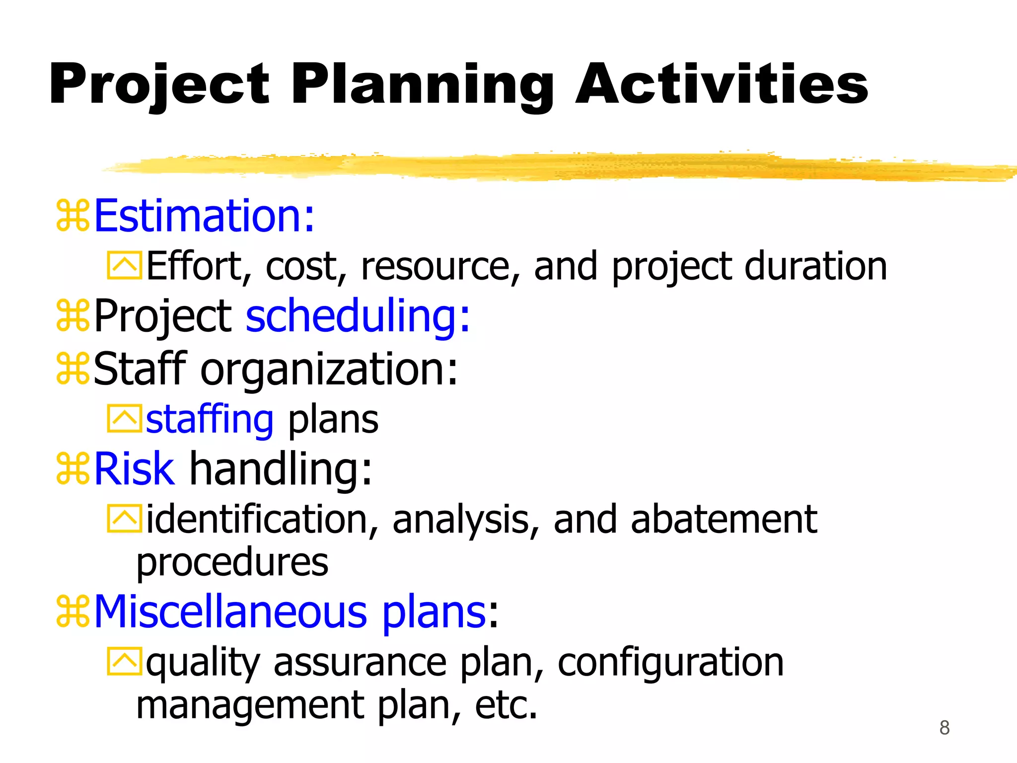
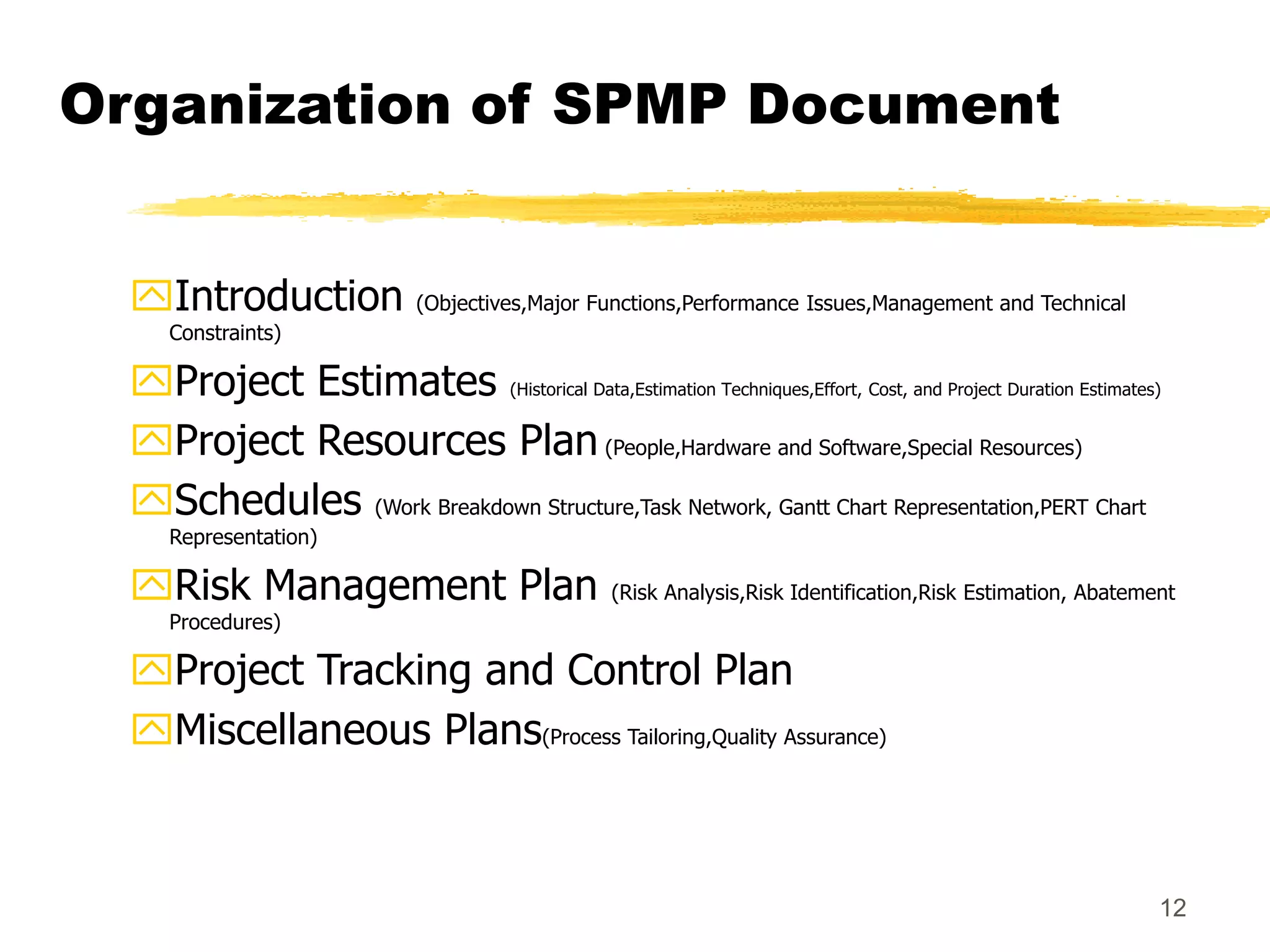
1. 1
Software Project
Management (Lecture 9)
Dr. R. Mall

2. 2
Organization of this
Lecture:
 Introduction to Project Planning
 Software Cost Estimation
Cost Estimation Models
Software Size Metrics
Empirical Estimation
Heuristic Estimation
COCOMO
 Staffing Level Estimation
 Effect of Schedule Compression on Cost
 Summary

3. 3
Introduction
Many software projects fail:
due to faulty project
management practices:
It is important to learn
different aspects of software
project management.

4. 4
Introduction
Goal of software project
management:
enable a group of engineers to
work efficiently towards successful
completion of a software project.

5. 5
Responsibility of project
managers
Project proposal writing,
Project cost estimation,
Scheduling,
Project staffing,
Project monitoring and control,
Software configuration management,
Risk management,
Managerial report writing and presentations, etc.

6. 6
Introduction
A project manager’s activities
are varied.
can be broadly classified into:
project planning,
project monitoring and control
activities.

7. 7
Project Planning
Once a project is found to be
feasible,
project managers undertake
project planning.

8. 8
Project Planning Activities
Estimation:
Effort, cost, resource, and project duration
Project scheduling:
Staff organization:
staffing plans
Risk handling:
identification, analysis, and abatement
procedures
Miscellaneous plans:
quality assurance plan, configuration
management plan, etc.

9. 9
Project planning
Requires utmost care and attention ---
commitments to unrealistic time and
resource estimates result in:
irritating delays.
customer dissatisfaction
adverse affect on team morale
poor quality work
project failure.

10. 10
Sliding Window Planning
Involves project planning over
several stages:
protects managers from making big
commitments too early.
More information becomes
available as project progresses.
Facilitates accurate planning

11. 11
SPMP Document
After planning is complete:
 Document the plans:
in a Software Project
Management Plan(SPMP)
document.

12. 12
Organization of SPMP Document
Introduction (Objectives,Major Functions,Performance Issues,Management and Technical
Constraints)
Project Estimates (Historical Data,Estimation Techniques,Effort, Cost, and Project Duration Estimates)
Project Resources Plan (People,Hardware and Software,Special Resources)
Schedules (Work Breakdown Structure,Task Network, Gantt Chart Representation,PERT Chart
Representation)
Risk Management Plan (Risk Analysis,Risk Identification,Risk Estimation, Abatement
Procedures)
Project Tracking and Control Plan
Miscellaneous Plans(Process Tailoring,Quality Assurance)

13. 13
Software Cost Estimation
Determine size of the product.
From the size estimate,
determine the effort needed.
From the effort estimate,
determine project duration, and cost.

14. 14
Size
Estimation
Effort
Estimation
Cost
Estimation
Duration
Estimation
Staffing
Estimation
Scheduling
Software Cost Estimation

15. 15
Software Cost Estimation
Three main approaches to
estimation:
Empirical
Heuristic
Analytical

16. 16
Software Cost Estimation
Techniques
Empirical techniques:
an educated guess based on past experience.
Heuristic techniques:
assume that the characteristics to be
estimated can be expressed in terms of
some mathematical expression.
Analytical techniques:
derive the required results starting from
certain simple assumptions.

17. 17
Software Size Metrics
LOC (Lines of Code):
Simplest and most widely used
metric.
Comments and blank lines should
not be counted.

18. 18
Disadvantages of Using LOC
Size can vary with coding style.
Focuses on coding activity alone.
Correlates poorly with quality and
efficiency of code.
Penalizes higher level
programming languages, code
reuse, etc.

19. 19
Disadvantages of Using LOC
(cont...)
Measures lexical/textual
complexity only.
does not address the issues of
structural or logical complexity.
Difficult to estimate LOC from
problem description.
So not useful for project planning

20. 20
Function Point Metric
Overcomes some of the shortcomings of
the LOC metric
Proposed by Albrecht in early 80's:
FP=4 #inputs + 5 #Outputs + 4
#inquiries + 10 #files + 10 #interfaces
Input:
A set of related inputs is counted as one input.

21. 21
Function Point Metric
Output:
A set of related outputs is counted as one output.
Inquiries:
Each user query type is counted.
Files:
Files are logically related data and thus can be data
structures or physical files.
Interface:
Data transfer to other systems.

22. 22
Function Point Metric(CONT.)
Suffers from a major drawback:
the size of a function is considered to
be independent of its complexity.
Extend function point metric:
 Feature Point metric:
considers an extra parameter:
Algorithm Complexity.

23. 23
Function Point Metric(CONT.)
Proponents claim:
FP is language independent.
Size can be easily derived from problem
description
Opponents claim:
it is subjective --- Different people can
come up with different estimates for the
same problem.

24. 24
Empirical Size Estimation
Techniques
Expert Judgement:
An euphemism for guess made by
an expert.
Suffers from individual bias.
Delphi Estimation:
overcomes some of the problems
of expert judgement.

25. 25
Expert judgement
Experts divide a software product into
component units:
e.g. GUI, database module, data
communication module, billing module,
etc.
Add up the guesses for each of the
components.

26. 26
Delphi Estimation:
Team of Experts and a coordinator.
Experts carry out estimation
independently:
mention the rationale behind their
estimation.
coordinator notes down any
extraordinary rationale:
circulates among experts.

27. 27
Delphi Estimation:
Experts re-estimate.
Experts never meet each other
 to discuss their viewpoints.

28. 28
Heuristic Estimation Techniques
Single Variable Model:
Parameter to be Estimated=C1(Estimated
Characteristic)d1
Multivariable Model:
Assumes that the parameter to be
estimated depends on more than one
characteristic.
Parameter to be Estimated=C1(Estimated
Characteristic)d1+ C2(Estimated Characteristic)d2+…
Usually more accurate than single
variable models.

29. 29
COCOMO Model
COCOMO (COnstructive COst MOdel)
proposed by Boehm.
Divides software product
developments into 3 categories:
Organic
Semidetached
Embedded

30. 30
COCOMO Product classes
Roughly correspond to:
application, utility and system programs
respectively.
Data processing and scientific programs
are considered to be application programs.
Compilers, linkers, editors, etc., are utility
programs.
Operating systems and real-time system
programs, etc. are system programs.

31. 31
Elaboration of Product
classes
Organic:
Relatively small groups
working to develop well-understood applications.
Semidetached:
Project team consists of a mixture of
experienced and inexperienced staff.
Embedded:
The software is strongly coupled to complex
hardware, or real-time systems.

32. 32
COCOMO Model(CONT.)
For each of the three product categories:
From size estimation (in KLOC), Boehm provides
equations to predict:
project duration in months
effort in programmer-months
Boehm obtained these equations:
examined historical data collected from a
large number of actual projects.

33. 33
COCOMO Model(CONT.)
Software cost estimation is done
through three stages:
Basic COCOMO,
Intermediate COCOMO,
Complete COCOMO.

34. 34
Basic COCOMO Model(CONT.)
Gives only an approximate estimation:
Effort = a1 (KLOC)a2
Tdev = b1 (Effort)b2
KLOC is the estimated kilo lines of source
code,
a1,a2,b1,b2 are constants for different
categories of software products,
Tdev is the estimated time to develop the
software in months,
Effort estimation is obtained in terms of
person months (PMs).

35. 35
Development Effort
Estimation
Organic :
 Effort = 2.4 (KLOC)1.05 PM
 Semi-detached:
Effort = 3.0(KLOC)1.12 PM
 Embedded:
Effort = 3.6 (KLOC)1.20PM

36. 36
Development Time
Estimation
Organic:
Tdev = 2.5 (Effort)0.38 Months
Semi-detached:
Tdev = 2.5 (Effort)0.35 Months
Embedded:
Tdev = 2.5 (Effort)0.32 Months

37. 37
Basic COCOMO Model(CONT.)
Effort is
somewhat
super-linear in
problem size.
Effort
Size

38. 38
Basic COCOMO Model(CONT.)
Development time
sublinear function of
product size.
When product size
increases two times,
development time
does not double.
Time taken:
almost same for all
the three product
categories.
Size
Dev. Time
60K
18 Months
14 Months
30K

39. 39
Basic COCOMO Model(CONT.)
Development time does not
increase linearly with product size:
For larger products more parallel
activities can be identified:
can be carried out simultaneously by
a number of engineers.

40. 40
Basic COCOMO Model(CONT.)
Development time is roughly the same for
all the three categories of products:
For example, a 60 KLOC program can be
developed in approximately 18 months
regardless of whether it is of organic, semi-
detached, or embedded type.
There is more scope for parallel activities for
system and application programs,
than utility programs.

41. 41
Example
The size of an organic software product has
been estimated to be 32,000 lines of source
code.
Effort = 2.4*(32)1.05 = 91 PM
Nominal development time = 2.5*(91)0.38 = 14
months

42. 42
Intermediate COCOMO
Basic COCOMO model assumes
effort and development time depend on
product size alone.
However, several parameters affect effort
and development time:
Reliability requirements
Availability of CASE tools and modern facilities to
the developers
Size of data to be handled

43. 43
Intermediate COCOMO
For accurate estimation,
the effect of all relevant parameters
must be considered:
Intermediate COCOMO model
recognizes this fact:
refines the initial estimate obtained by the
basic COCOMO by using a set of 15 cost
drivers (multipliers).

44. 44
Intermediate COCOMO
(CONT.)
If modern programming practices
are used,
initial estimates are scaled
downwards.
If there are stringent reliability
requirements on the product :
initial estimate is scaled upwards.

45. 45
Intermediate COCOMO
(CONT.)
Rate different parameters on a
scale of one to three:
Depending on these ratings,
multiply cost driver values with
the estimate obtained using the
basic COCOMO.

46. 46
Intermediate COCOMO
(CONT.)
Cost driver classes:
Product: Inherent complexity of the product,
reliability requirements of the product, etc.
Computer: Execution time, storage
requirements, etc.
Personnel: Experience of personnel, etc.
Development Environment: Sophistication of
the tools used for software development.

47. 47
Shortcoming of basic and
intermediate COCOMO models
Both models:
consider a software product as a single
homogeneous entity:
However, most large systems are made up of
several smaller sub-systems.
Some sub-systems may be considered as organic
type, some may be considered embedded, etc.
for some the reliability requirements may be high,
and so on.

48. 48
Complete COCOMO
Cost of each sub-system is estimated
separately.
Costs of the sub-systems are added
to obtain total cost.
Reduces the margin of error in the
final estimate.

49. 49
Complete COCOMO
Example
A Management Information System (MIS) for an
organization having offices at several places
across the country:
Database part (semi-detached)
Graphical User Interface (GUI) part (organic)
Communication part (embedded)
Costs of the components are estimated
separately:
summed up to give the overall cost of the system.

50. 50
Halstead's Software
Science
An analytical technique to
estimate:
size,
development effort,
development time.

51. 51
Halstead's Software
Science
Halstead used a few primitive program
parameters
number of operators and operands
Derived expressions for:
over all program length,
potential minimum volume
actual volume,
language level,
effort, and
development time.

52. 52
Staffing Level Estimation
Number of personnel required during
any development project:
not constant.
Norden in 1958 analyzed many R&D
projects, and observed:
Rayleigh curve represents the number
of full-time personnel required at any
time.

53. 53
Rayleigh Curve
Rayleigh curve is
specified by two
parameters:
td the time at
which the curve
reaches its
maximum
K the total area
under the curve.
L=f(K, td)
Effort
Time
td
Rayleigh Curve

54. 54
Putnam’s Work:
In 1976, Putnam studied the problem of
staffing of software projects:
observed that the level of effort required in
software development efforts has a similar
envelope.
found that the Rayleigh-Norden curve
relates the number of delivered lines of code to
effort and development time.

55. 55
Putnam’s Work(CONT.):
Putnam analyzed a large number of
army projects, and derived the
expression:
L=CkK1/3td4/3
K is the effort expended and L is the
size in KLOC.
td is the time to develop the software.
Ck is the state of technology constant
reflects factors that affect programmer
productivity.

56. 56
Putnam’s Work(CONT.):
Ck=2 for poor development environment
no methodology, poor documentation, and
review, etc.
Ck=8 for good software development
environment
software engineering principles used
Ck=11 for an excellent environment

57. 57
Rayleigh Curve
Very small number of engineers are
needed at the beginning of a project
 carry out planning and specification.
As the project progresses:
more detailed work is required,
number of engineers slowly increases
and reaches a peak.

58. 58
Rayleigh Curve
Putnam observed that:
the time at which the Rayleigh curve
reaches its maximum value
corresponds to system testing and product
release.
After system testing,
the number of project staff falls till product
installation and delivery.

59. 59
Rayleigh Curve
From the Rayleigh curve observe
that:
approximately 40% of the area
under the Rayleigh curve is to the
left of td
and 60% to the right.

60. 60
Effect of Schedule Change
on Cost
Using the Putnam's expression for L,
K=L3/Ck3td4
Or, K=C1/td4
For the same product size,
C1=L3/Ck3 is a constant.
Or, K1/K2 = td24/td14

61. 61
Effect of Schedule Change on
Cost(CONT.)
Observe:
a relatively small compression in
delivery schedule
can result in substantial penalty on human
effort.
Also, observe:
benefits can be gained by using fewer
people over a somewhat longer time
span.

62. 62
Example
If the estimated development time is
1 year, then in order to develop the
product in 6 months,
the total effort and hence the cost
increases 16 times.
In other words,
the relationship between effort and the
chronological delivery time is highly
nonlinear.

63. 63
Effect of Schedule Change on
Cost(CONT.)
Putnam model indicates extreme penalty
for schedule compression
and extreme reward for expanding the
schedule.
Putnam estimation model works
reasonably well for very large systems,
but seriously overestimates the effort for
medium and small systems.

64. 64
Effect of Schedule Change on
Cost(CONT.)
Boehm observed:
“There is a limit beyond which the
schedule of a software project cannot
be reduced by buying any more
personnel or equipment.”
This limit occurs roughly at 75% of the
nominal time estimate.

65. 65
Effect of Schedule Change
on Cost(CONT.)
If a project manager accepts a customer
demand to compress the development
time by more than 25%
very unlikely to succeed.
every project has only a limited amount of parallel
activities
sequential activities cannot be speeded up by
hiring any number of additional engineers.
many engineers have to sit idle.

66. 66
Jensen Model
Jensen model is very similar to
Putnam model.
attempts to soften the effect of
schedule compression on effort
makes it applicable to smaller and
medium sized projects.

67. 67
Jensen Model
Jensen proposed the equation:
L=CtetdK1/2
Where,
Cte is the effective technology constant,
td is the time to develop the software, and
K is the effort needed to develop the
software.

68. 68
Organization Structure
Functional Organization:
Engineers are organized into functional
groups, e.g.
specification, design, coding, testing,
maintenance, etc.
Engineers from functional groups get
assigned to different projects

69. 69
Advantages of Functional
Organization
Specialization
Ease of staffing
Good documentation is produced
different phases are carried out by
different teams of engineers.
Helps identify errors earlier.

70. 70
Project Organization
Engineers get assigned to a project
for the entire duration of the project
Same set of engineers carry out all the
phases
Advantages:
Engineers save time on learning details
of every project.
Leads to job rotation

71. 71
Team Structure
Problems of different complexities
and sizes require different team
structures:
Chief-programmer team
Democratic team
Mixed organization

72. 72
Democratic Teams
Suitable for:
small projects requiring less than five or
six engineers
research-oriented projects
A manager provides administrative
leadership:
at different times different members of
the group provide technical leadership.

73. 73
Democratic Teams
Democratic organization provides
higher morale and job satisfaction to the
engineers
 therefore leads to less employee turnover.
Suitable for less understood problems,
a group of engineers can invent better
solutions than a single individual.

74. 74
Democratic Teams
Disadvantage:
team members may waste a
lot time arguing about trivial
points:
absence of any authority in the
team.

75. 75
Chief Programmer Team
A senior engineer provides
technical leadership:
partitions the task among the team
members.
verifies and integrates the products
developed by the members.

76. 76
Chief Programmer Team
Works well when
the task is well understood
also within the intellectual grasp of a single
individual,
importance of early completion
outweighs other factors
team morale, personal development, etc.

77. 77
Chief Programmer Team
Chief programmer team is subject to
single point failure:
too much responsibility and authority is
assigned to the chief programmer.

78. 78
Mixed Control Team
Organization
Draws upon ideas from both:
democratic organization and
chief-programmer team organization.
Communication is limited
to a small group that is most likely to benefit
from it.
Suitable for large organizations.

79. 79
Team Organization
Chief Programmer team
Democratic Team

80. 80
Mixed team organization

81. 81
Summary
We discussed the broad
responsibilities of the project
manager:
Project planning
Project Monitoring and Control

82. 82
Summary
To estimate software cost:
Determine size of the product.
Using size estimate,
determine effort needed.
From the effort estimate,
determine project duration, and cost.

83. 83
Summary(CONT.)
Cost estimation techniques:
Empirical Techniques
Heuristic Techniques
Analytical Techniques
Empirical techniques:
based on systematic guesses by experts.
Expert Judgement
Delphi Estimation

84. 84
Summary(CONT.)
Heuristic techniques:
assume that characteristics of a software
product can be modeled by a mathematical
expression.
COCOMO
Analytical techniques:
derive the estimates starting with some basic
assumptions:
Halstead's Software Science

85. 85
Summary(CONT.)
The staffing level during the life cycle of a
software product development:
follows Rayleigh curve
maximum number of engineers required
during testing.

86. 86
Summary(CONT.)
Relationship between schedule change and
effort:
highly nonlinear.
Software organizations are usually
organized in:
functional format
project format

87. 87
Summary(CONT.)
Project teams can be organized in
following ways:
Chief programmer: suitable for routine work.
Democratic: Small teams doing R&D type
work
Mixed: Large projects