Download as PPSX, PPTX

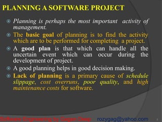
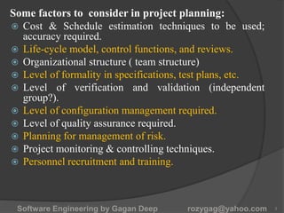


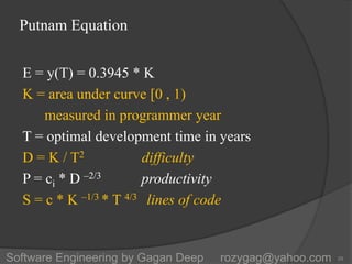


The document discusses software cost estimation and planning. It describes several models for software cost estimation including COCOMO and Putnam models. COCOMO uses staff months and lines of code to initially estimate effort which is then adjusted based on cost drivers. Putnam uses a Rayleigh curve staffing model based on volume, difficulty, and time constraints. Thorough planning is important to software projects and factors like life cycle, quality assurance, and risk management should be considered. Historical data and validated models can help produce more accurate cost and schedule estimates.