kalmanian domain introduction is provided.

1. 1
Introduction to Kalman Filters
Michael Williams
5 June 2003

2. 2
Overview
• The Problem – Why do we need Kalman
Filters?
• What is a Kalman Filter?
• Conceptual Overview
• The Theory of Kalman Filter
• Simple Example

3. 3
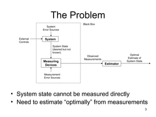
The Problem
• System state cannot be measured directly
• Need to estimate “optimally” from measurements
Measuring
Devices Estimator
Measurement
Error Sources
System State
(desired but not
known)
External
Controls
Observed
Measurements
Optimal
Estimate of
System State
System
Error Sources
System
Black Box

4. 4
What is a Kalman Filter?
• Recursive data processing algorithm
• Generates optimal estimate of desired quantities
given the set of measurements
• Optimal?
– For linear system and white Gaussian errors, Kalman
filter is “best” estimate based on all previous
measurements
– For non-linear system optimality is ‘qualified’
• Recursive?
– Doesn’t need to store all previous measurements and
reprocess all data each time step

5. 5
Conceptual Overview
• Simple example to motivate the workings
of the Kalman Filter
• Theoretical Justification to come later – for
now just focus on the concept
• Important: Prediction and Correction

6. 6
Conceptual Overview
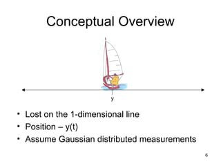
• Lost on the 1-dimensional line
• Position – y(t)
• Assume Gaussian distributed measurements
y

7. 7
Conceptual Overview
0 10 20 30 40 50 60 70 80 90 100
0
0.02
0.04
0.06
0.08
0.1
0.12
0.14
0.16
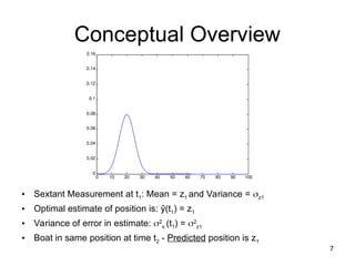
• Sextant Measurement at t1: Mean = z1 and Variance = z1
• Optimal estimate of position is: ŷ(t1) = z1
• Variance of error in estimate: 2
x (t1) = 2
z1
• Boat in same position at time t2 - Predicted position is z1

8. 8
0 10 20 30 40 50 60 70 80 90 100
0
0.02
0.04
0.06
0.08
0.1
0.12
0.14
0.16
Conceptual Overview
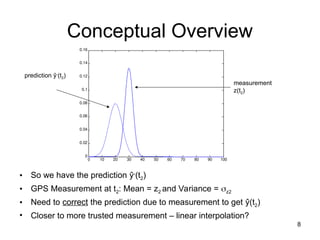
• So we have the prediction ŷ-
(t2)
• GPS Measurement at t2: Mean = z2 and Variance = z2
• Need to correct the prediction due to measurement to get ŷ(t2)
• Closer to more trusted measurement – linear interpolation?
prediction ŷ-
(t2)
measurement
z(t2)

9. 9
0 10 20 30 40 50 60 70 80 90 100
0
0.02
0.04
0.06
0.08
0.1
0.12
0.14
0.16
Conceptual Overview
• Corrected mean is the new optimal estimate of position
• New variance is smaller than either of the previous two variances
measurement
z(t2)
corrected optimal
estimate ŷ(t2)
prediction ŷ-
(t2)

10. 10
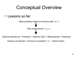
Conceptual Overview
• Lessons so far:
Make prediction based on previous data - ŷ-
, -
Take measurement – zk, z
Optimal estimate (ŷ) = Prediction + (Kalman Gain) * (Measurement - Prediction)
Variance of estimate = Variance of prediction * (1 – Kalman Gain)

11. 11
0 10 20 30 40 50 60 70 80 90 100
0
0.02
0.04
0.06
0.08
0.1
0.12
0.14
0.16
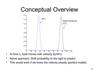
Conceptual Overview
• At time t3, boat moves with velocity dy/dt=u
• Naïve approach: Shift probability to the right to predict
• This would work if we knew the velocity exactly (perfect model)
ŷ(t2)
Naïve Prediction
ŷ-
(t3)

12. 12
0 10 20 30 40 50 60 70 80 90 100
0
0.02
0.04
0.06
0.08
0.1
0.12
0.14
0.16
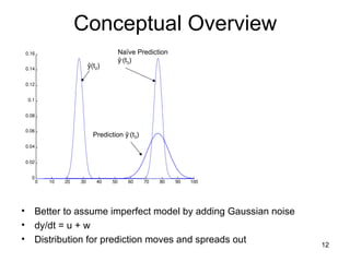
Conceptual Overview
• Better to assume imperfect model by adding Gaussian noise
• dy/dt = u + w
• Distribution for prediction moves and spreads out
ŷ(t2)
Naïve Prediction
ŷ-
(t3)
Prediction ŷ-
(t3)

13. 13
0 10 20 30 40 50 60 70 80 90 100
0
0.02
0.04
0.06
0.08
0.1
0.12
0.14
0.16
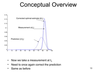
Conceptual Overview
• Now we take a measurement at t3
• Need to once again correct the prediction
• Same as before
Prediction ŷ-
(t3)
Measurement z(t3)
Corrected optimal estimate ŷ(t3)

14. 14
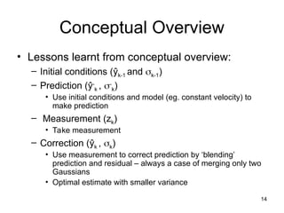
Conceptual Overview
• Lessons learnt from conceptual overview:
– Initial conditions (ŷk-1 and k-1)
– Prediction (ŷ-
k , -
k)
• Use initial conditions and model (eg. constant velocity) to
make prediction
– Measurement (zk)
• Take measurement
– Correction (ŷk , k)
• Use measurement to correct prediction by ‘blending’
prediction and residual – always a case of merging only two
Gaussians
• Optimal estimate with smaller variance

15. 15
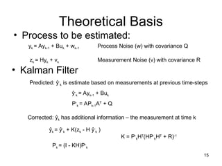
Theoretical Basis
• Process to be estimated:
yk = Ayk-1 + Buk + wk-1
zk = Hyk + vk
Process Noise (w) with covariance Q
Measurement Noise (v) with covariance R
• Kalman Filter
Predicted: ŷ-
k is estimate based on measurements at previous time-steps
ŷk = ŷ-
k + K(zk - H ŷ-
k )
Corrected: ŷk has additional information – the measurement at time k
K = P-
kHT
(HP-
kHT
+ R)-1
ŷ-
k = Ayk-1 + Buk
P-
k = APk-1AT
+ Q
Pk = (I - KH)P-
k

16. 16
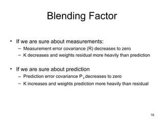
Blending Factor
• If we are sure about measurements:
– Measurement error covariance (R) decreases to zero
– K decreases and weights residual more heavily than prediction
• If we are sure about prediction
– Prediction error covariance P-
k decreases to zero
– K increases and weights prediction more heavily than residual

17. 17
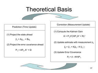
Theoretical Basis
ŷ-
k = Ayk-1 + Buk
P-
k = APk-1AT
+ Q
Prediction (Time Update)
(1) Project the state ahead
(2) Project the error covariance ahead
Correction (Measurement Update)
(1) Compute the Kalman Gain
(2) Update estimate with measurement zk
(3) Update Error Covariance
ŷk = ŷ-
k + K(zk - H ŷ-
k )
K = P-
kHT
(HP-
kHT
+ R)-1
Pk = (I - KH)P-
k

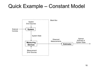
18. 18
Quick Example – Constant Model
Measuring
Devices Estimator
Measurement
Error Sources
System State
External
Controls
Observed
Measurements
Optimal
Estimate of
System State
System
Error Sources
System
Black Box

19. 19
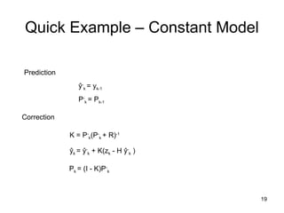
Quick Example – Constant Model
Prediction
ŷk = ŷ-
k + K(zk - H ŷ-
k )
Correction
K = P-
k(P-
k + R)-1
ŷ-
k = yk-1
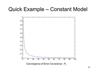
P-
k = Pk-1
Pk = (I - K)P-
k

20. 20
Quick Example – Constant Model
0 10 20 30 40 50 60 70 80 90 100
-0.7
-0.6
-0.5
-0.4
-0.3
-0.2
-0.1
0

21. 21
Quick Example – Constant Model
0 10 20 30 40 50 60 70 80 90 100
0
0.1
0.2
0.3
0.4
0.5
0.6
0.7
0.8
0.9
1
Convergence of Error Covariance - Pk

22. 22
0 10 20 30 40 50 60 70 80 90 100
-0.7
-0.6
-0.5
-0.4
-0.3
-0.2
-0.1
0
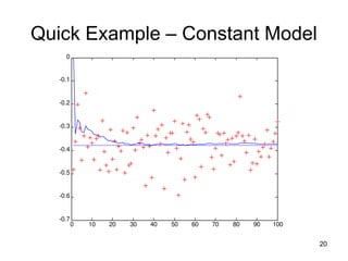
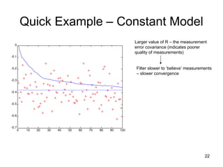
Quick Example – Constant Model
Larger value of R – the measurement
error covariance (indicates poorer
quality of measurements)
Filter slower to ‘believe’ measurements
– slower convergence

23. 23
References
1. Kalman, R. E. 1960. “A New Approach to Linear Filtering and Prediction
Problems”, Transaction of the ASME--Journal of Basic Engineering, pp. 35-45
(March 1960).
2. Maybeck, P. S. 1979. “Stochastic Models, Estimation, and Control, Volume 1”,
Academic Press, Inc.
3. Welch, G and Bishop, G. 2001. “An introduction to the Kalman Filter”,
http://www.cs.unc.edu/~welch/kalman/