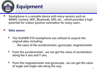
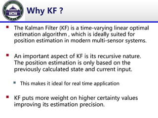
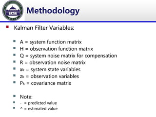
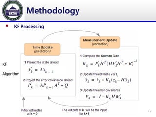
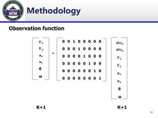
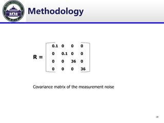
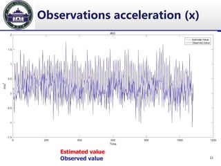
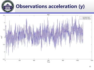
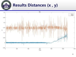
The document discusses the use of Kalman filters for position estimation, particularly utilizing smartphone sensors for indoor positioning applications. It emphasizes the importance of precise indoor location tracking, given that people spend most of their time indoors, and outlines the methodology for processing data from smartphones like the Huawei P10. The study concludes with potential improvements for accuracy and the importance of various calibration methods.

1. 1
Position Estimation in Kalman Filter
Presented By
David Sestak, Zhang zhen bing,
Ahmed Mohamed Reda & Mohamed Freeshah
January, 2018

2. 2
Position Estimation in Kalman Filter
Zhang zhen bing
Presented By
Ahmed Mohamed
Reda
Mohamed Ahmed FreeshahDavid Sestak

3. 3
▪ Introduction
▪ Motivation
▪ Equipment
▪ Methodology
➢ Data source
➢ KF Processing
▪ Results
Project Schedule

4. 4
▪ Precise position estimation is one of the fundamental
technical dependencies in our society today. It has
influenced our lives in countless ways most people do
not think about.
▪ It is used in a variety of applications including:
▪ GNSS (and all its varying applications)
▪ Self driving vehicles
▪ Mobile robots
▪ Internet of Things (IoT) and many others
Introduction

5. 5
▪ Indoor positioning has become an area of increasing
interest utilizing the various signals that our devices
use such as Bluetooth and WiFi.
▪ People spend about 80% of their time indoors, so it is
of great significant to achieve precise indoor position
estimation.
▪ This is why we are using a smartphone, a device
everyone carries, for real time position estimation only
using its inertial sensors.
Motivation

6. 6
▪ Smartphone is a versatile device with many sensors such as:
MEMS, Camera, WiFi, Bluetooth, GPS, etc. , which provides a high
potential for indoor position estimation for many users .
▪ Data source
▪ The HUAWEI P10 smartphone was utilized to acquire the
original data, including:
the value of the accelerometer, gyroscope, magnetometer
▪ From the accelerometer , we can get the value of acceleration
along the X axis and Y axis.
▪ From the magnetometer and gyroscope , we can get the value
of angle and angle rate along the way.
Equipment

7. 7
HUAWEI P10 Sensors:
▪ Fingerprint Sensor, G-Sensor, Gyroscope Sensor,
Compass, Ambient Light Sensor, Proximity Sensor,
Hall Sensor
Software:
▪ HIPE2.3
▪ MATLAB
Equipment

8. 8
▪ The Kalman Filter (KF) is a time-varying linear optimal
estimation algorithm , which is ideally suited for
position estimation in modern multi-sensor systems.
▪ An important aspect of KF is its recursive nature.
The position estimation is only based on the
previously calculated state and current input.
▪ This makes it ideal for real time application
▪ KF puts more weight on higher certainty values
improving its estimation precision.
Why KF ?

9. 9
▪ Our Observation Variables:
▪ ax = x-direction acceleration
▪ ay = y-direction acceleration
▪ θ = direction
▪ ω = angular rate
▪ These are the observation values that our
smartphone inertial sensors provides.
Methodology

10. 10
▪ Kalman Filter Variables:
▪ A = system function matrix
▪ H = observation function matrix
▪ Q = system noise matrix for compensation
▪ R = observation noise matrix
▪ xk = system state variables
▪ zk = observation variables
▪ Pk = covariance matrix
▪ Note:
▪ - = predicted value
▪ ^ = estimated value
Methodology

11. 11
▪ KF Processing
Methodology
KF
Algorithm

12. 12
Methodology
0
1
2
3
4
5
6
类别 1 类别 2 类别 3 类别 4

13. 13
▪ KF Processing
In our project:
Assumption:(Gaussian distribution)
First: define the state variables
Second: confirm the system function according to the physic
principle.
Third: given the observation equation.
Fourth: confirm the matrix of Q, R, and P according to the
experience.
Methodology

14. 14
Methodology
K+1 K
0 0 t 0 0 0 0 0
0 0 0 t 0 0 0 0
0 0 1 0 t 0 0 0
0 0 0 1 0 t 0 0
0 0 0 0 1 0 0 0
0 0 0 0 0 1 0 0
0 0 0 0 0 0 1 t
0 0 0 0 0 0 0 1
θ
ω
θ
ω
=
System function

15. 15
Methodology
K+1 K+1
θ
ω
0 0 0 0 1 0 0 0
0 0 0 0 0 1 0 0
0 0 0 0 0 0 1 0
0 0 0 0 0 0 0 1
θ
ω
=
Observation function

16. 16
Methodology
K+1 K+1
θ
ω
0 0 1 0 0 0 0 0
0 0 0 1 0 0 0 0
0 0 0 0 1 0 0 0
0 0 0 0 0 1 0 0
0 0 0 0 0 0 1 0
0 0 0 0 0 0 0 1
θ
ω
=
Observation function

17. 17
Methodology
0.3 0 0 0 0 0 0 0
0 0.3 0 0 0 0 0 0
0 0 0.01 0 0 0 0 0
0 0 0 0.01 0 0 0 0
0 0 0 0 0.01 0 0 0
0 0 0 0 0 0.01 0 0
0 0 0 0 0 0 16 0
0 0 0 0 0 0 0 16
Q =
Covariance matrix of the system noise

18. 18
Methodology
0.1 0 0 0
0 0.1 0 0
0 0 36 0
0 0 0 36
R =
Covariance matrix of the measurement noise

19. 19
Methodology
0.01 0 0 0 0 0
0 0.01 0 0 0 0
0 0 0.1 0 0 0
0 0 0 0.1 0 0
0 0 0 0 36 0
0 0 0 0 0 36
R =
Covariance matrix of the measurement noise

20. 20
Methodology
1 0 0 0 0 0 0 0
0 1 0 0 0 0 0 0
0 0 0.1 0 0 0 0 0
0 0 0 0.1 0 0 0 0
0 0 0 0 0.1 0 0 0
0 0 0 0 0 0.1 0 0
0 0 0 0 0 0 36 0
0 0 0 0 0 0 0 36
P =
Error covariance matrix of the estimation of the state variables

21. 21
Observations acceleration (x)
Estimated value
Observed value

22. 22
Observations acceleration (y)

23. 23
Observations yaw angle

24. 24
Observations Angle Rate

25. 25
Observations Velocity (x , y)

26. 26
Results Distances (x , y)

27. 27
Results Sys. Variables Variance

28. 28
Results Final Track
Part of play ground in front of LIESMARS
(Straight line = 100 m, Curve = 50 m)

29. 29
▪ Errors:
▪ Unreasonable velocity increase
▪ Improvement used:
▪ Counteracting unreasonable velocity increase
▪ Ways to Improve:
▪ Ground Truth
▪ Inertial sensor position update
Discussion

30. 30
Conclusion
Availability
Continuity
Accuracy
Integrity
(Ways to Improve by four criteria)

31. 31
▪ Leick, A. L. Rapoport, D. Tatarnikov., 2016, GPS
Satellite Surveying, 4th Edition, New York: John
Wiley and Sons
▪ G. Welch, G. Bishop., 2001, An Introduction to the
Kalman Filter, University of North Carolina at Chapel
Hill, Department of Computer Science, Chapel Hill,
NC 27599-3175 ( http://www.cs.unc.edu )
▪ Kalman, R.E. Trans ASME. 1960; 82:35–45. Crossref |
Scopus (12465)
▪ http://consumer.huawei.com/en/phones/p10/specs/
Major References:

32. 32
Thank You !