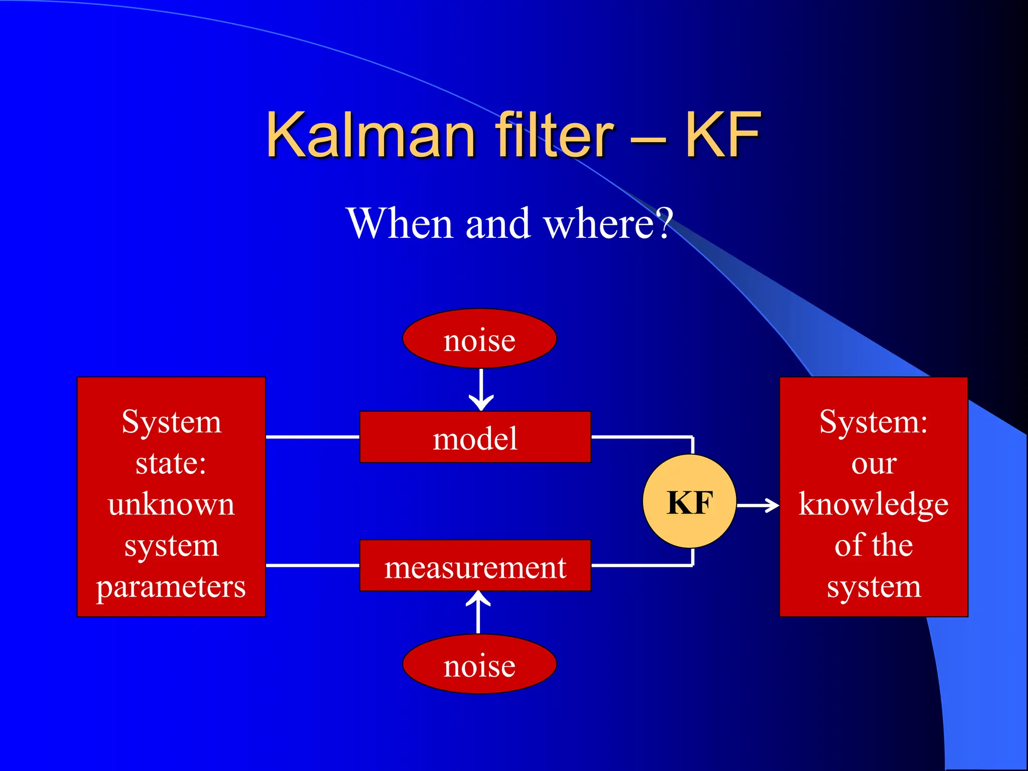
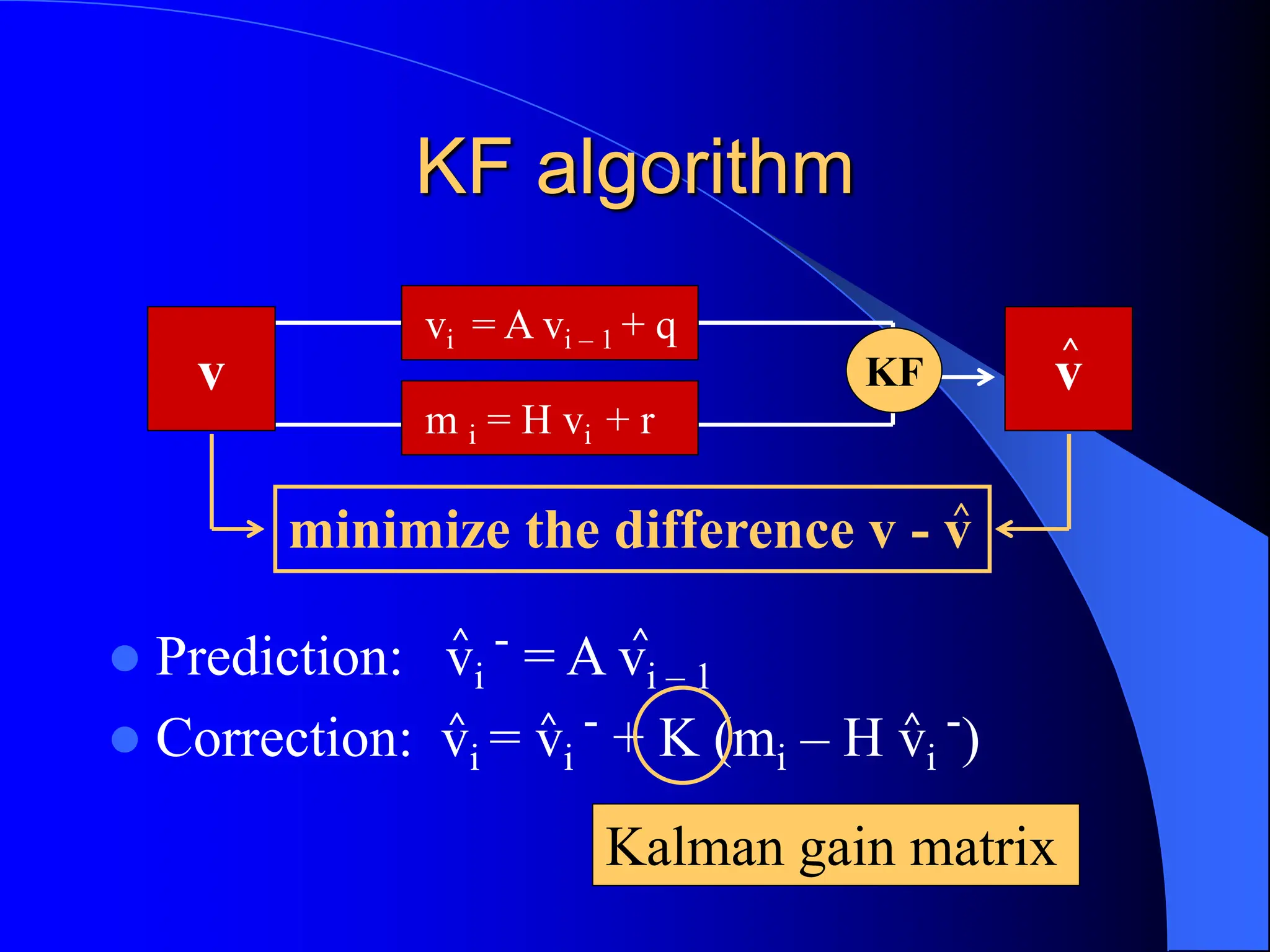
Using Kalman Filter to
Track Particles
Saša Fratina
advisor:
Samo Korpar
2004-01-13
Overview
 Motivation
 Basic principles of Kalman Filter
 example
 Application to particle tracking
No big deal
R. E. Kalman
 Born 1930 in Hungary
 Studied at MIT / Columbia
 Developed filter in 1960/61
i i + 1
Illustration example
Measuring parameters of a particle track in 2D
particle
track
parameters:
y, k
measurement:
m
System:
our
knowledge
of the
system
Kalman filter – KF
System
state:
unknown
system
parameters
model
measurement


noise
noise
?
KF
When and where?
When and where?
 Tracking and navigation
– Tracking missiles, aircrafts and spacecrafts
– GPS technology
– Visual reality
 Tracking in
HEP experiments
KF assumptions
 Linear system
– System parameters are linear
function of parameters at
some previous time
– Measurements are linear
function of parameters
 White Gaussian noise
– White: uncorrelated in time
– Gaussian: noise amplitude
 KF is the
optimal filter
KF description
System:
our
knowledge
of the
system
System
state:
unknown
system
parameters
model
measurement
KF
parameters
v
vi = A vi - 1
m i = H vi


noise
noise
+ qi
+ ri
using vectors and matrices
estimation
of
parameters
v
^
KF description: example
 System parameters: v
 System model:
linear motion y = k x
vi = A vi - 1
 Measurement model:
m i = H vi
1
i
k
y
1
0
Δx
1
i
k
y


























i
k
y
0
1
i
m 














i
k
y
i
v 








Noise
Noise: e
Noise covariance matrix
 System noise: vi = A vi – 1+ qi  Q = E(qqT)
 Measurement noise: m i = H vi + ri
 R = E(rrT)















)
e
E(e
)
e
E(e
)
e
E(e
)
e
E(e
)
E(ee
V 2
2
1
2
2
1
1
1
T
Gaussian  E(e2) = σ2
KF algorithm
 Prediction: vi
- = A vi – 1
 Correction: vi = vi
- + K (mi – H vi
-)
vi = A vi – 1 + q
m i = H vi + r
v
^
v KF
Kalman gain matrix
minimize the difference v - v
^
^
^ ^ ^
^
Kalman gain matrix
 It is easy to show
K = V-HT (H V-HT +R)-1,
where Vi
- = AVi-1AT + Q
 Minimize the expected error
 Limits:
– system noise << measurement noise  vi = vi
–
– system noise >> measurement noise  vi = H–1 mi
0
K
V
)
e
E(e
)
e
E(e
)
e
E(e
)
e
E(e
)
E(ee
V
;
v
v
e
ab
ij
2
2
1
2
2
1
1
1
T






















^ ^
^
Error on parameters
 Predictor: Vi
- = AVi-1AT + Q
– Q: system noise
 Corrector: Vi = (I - KH) Vi
-
– error reduced
Kalman filter
Least squares
Example
 Simulation
y = k x
 Implemented
KF
– prediction
– correction
 Compare with
LS method
x
y
System noise
x
y
Kalman filter
Least squares
 Matrix description of system state, model
and measurement
 Progressive method
 Proper dealing with noise
KF overview
prediction
correction
Application to particle tracking
 Detector:
– Silicon vertex detector
– Central drift
chamber
 Description
of track:
5 parameters
Advantages of using KF
in particle tracking
 Progressive method
– No large matrices has to be inverted
 Proper dealing with system noise
 Track finding and track fitting
 Detection of outliers
 Merging track from different segments
Modifications of KF
 (!) Non - linear
system  extended
Kalman filter
 Full precision only
after the last step
– Prediction
– Correction
– Smoothing
Kalman filter
Least squares
x
y
Conclusion
 We have demonstrated the principles
predictor – corrector method
combining model and measurement
 Very useful in tracking
 For given assumptions, KF is the optimal filter
 Extensions for non-linear systems
 Extensive application
To sum up…
Tracking in BELLE detector
Track finding
Track fitting
Track managing
Notation overview
 v: vector of parameters
– v: our estimation
– v-: predicted value
 m: vector of measurements
 A: matrix describing linear system  vi = A vi – 1
 H: matrix describing measurements  m i = H vi
 V: error (on parameter) covariance matrix
 Q: system noise covariance matrix
 R: measurement noise covariance matrix
 K: Kalman gain matrix
^

kalman filter illustrated with 2D example

  • 1.
    Using Kalman Filterto Track Particles Saša Fratina advisor: Samo Korpar 2004-01-13
  • 2.
    Overview  Motivation  Basicprinciples of Kalman Filter  example  Application to particle tracking No big deal
  • 3.
    R. E. Kalman Born 1930 in Hungary  Studied at MIT / Columbia  Developed filter in 1960/61
  • 4.
    i i +1 Illustration example Measuring parameters of a particle track in 2D particle track parameters: y, k measurement: m
  • 5.
    System: our knowledge of the system Kalman filter– KF System state: unknown system parameters model measurement   noise noise ? KF When and where?
  • 6.
    When and where? Tracking and navigation – Tracking missiles, aircrafts and spacecrafts – GPS technology – Visual reality  Tracking in HEP experiments
  • 7.
    KF assumptions  Linearsystem – System parameters are linear function of parameters at some previous time – Measurements are linear function of parameters  White Gaussian noise – White: uncorrelated in time – Gaussian: noise amplitude  KF is the optimal filter
  • 8.
    KF description System: our knowledge of the system System state: unknown system parameters model measurement KF parameters v vi= A vi - 1 m i = H vi   noise noise + qi + ri using vectors and matrices estimation of parameters v ^
  • 9.
    KF description: example System parameters: v  System model: linear motion y = k x vi = A vi - 1  Measurement model: m i = H vi 1 i k y 1 0 Δx 1 i k y                           i k y 0 1 i m                i k y i v         
  • 10.
    Noise Noise: e Noise covariancematrix  System noise: vi = A vi – 1+ qi  Q = E(qqT)  Measurement noise: m i = H vi + ri  R = E(rrT)                ) e E(e ) e E(e ) e E(e ) e E(e ) E(ee V 2 2 1 2 2 1 1 1 T Gaussian  E(e2) = σ2
  • 11.
    KF algorithm  Prediction:vi - = A vi – 1  Correction: vi = vi - + K (mi – H vi -) vi = A vi – 1 + q m i = H vi + r v ^ v KF Kalman gain matrix minimize the difference v - v ^ ^ ^ ^ ^ ^
  • 12.
    Kalman gain matrix It is easy to show K = V-HT (H V-HT +R)-1, where Vi - = AVi-1AT + Q  Minimize the expected error  Limits: – system noise << measurement noise  vi = vi – – system noise >> measurement noise  vi = H–1 mi 0 K V ) e E(e ) e E(e ) e E(e ) e E(e ) E(ee V ; v v e ab ij 2 2 1 2 2 1 1 1 T                       ^ ^ ^
  • 13.
    Error on parameters Predictor: Vi - = AVi-1AT + Q – Q: system noise  Corrector: Vi = (I - KH) Vi - – error reduced
  • 14.
    Kalman filter Least squares Example Simulation y = k x  Implemented KF – prediction – correction  Compare with LS method x y
  • 15.
  • 16.
     Matrix descriptionof system state, model and measurement  Progressive method  Proper dealing with noise KF overview prediction correction
  • 17.
    Application to particletracking  Detector: – Silicon vertex detector – Central drift chamber  Description of track: 5 parameters
  • 18.
    Advantages of usingKF in particle tracking  Progressive method – No large matrices has to be inverted  Proper dealing with system noise  Track finding and track fitting  Detection of outliers  Merging track from different segments
  • 19.
    Modifications of KF (!) Non - linear system  extended Kalman filter  Full precision only after the last step – Prediction – Correction – Smoothing Kalman filter Least squares x y
  • 20.
    Conclusion  We havedemonstrated the principles predictor – corrector method combining model and measurement  Very useful in tracking  For given assumptions, KF is the optimal filter  Extensions for non-linear systems  Extensive application To sum up…
  • 21.
    Tracking in BELLEdetector Track finding Track fitting Track managing
  • 22.
    Notation overview  v:vector of parameters – v: our estimation – v-: predicted value  m: vector of measurements  A: matrix describing linear system  vi = A vi – 1  H: matrix describing measurements  m i = H vi  V: error (on parameter) covariance matrix  Q: system noise covariance matrix  R: measurement noise covariance matrix  K: Kalman gain matrix ^