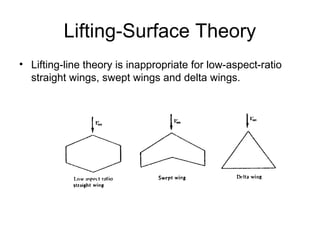
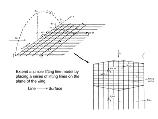
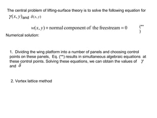
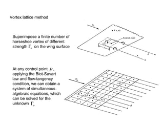
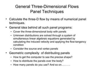
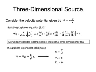
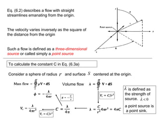
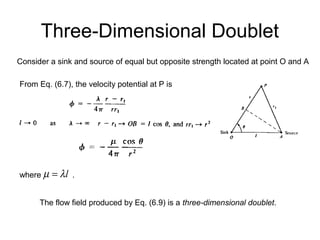
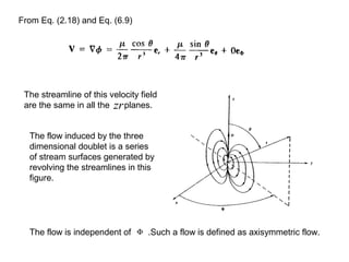
This document outlines concepts in three-dimensional fluid flow, including: 1) Lifting surface theory which extends lifting line theory to low aspect ratio wings by placing lifting lines across the wing surface. 2) The vortex lattice method which superimposes horseshoe vortices on the wing to obtain equations relating vortex strengths that satisfy flow tangency. 3) A three-dimensional source defined as a flow with radial streamlines emanating from a point, and a doublet defined as a sink and source of equal strength. 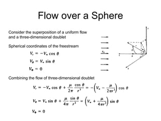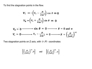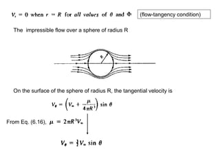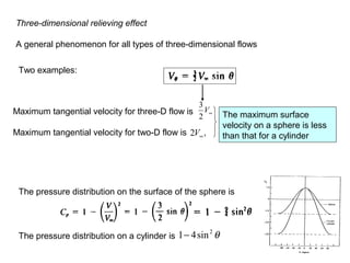4) Flow over a sphere is analyzed using a uniform flow and doublet, finding two stagnation points and that maximum surface velocity is less than over a cylinder, demonstrating three

1. c
CAREER POINT UNIVE
MAJOR ASSIGNMENT
Three-dimensional flow down strem
of axial flow fans

2. Outline
• Lifting-surface theory
• Vortex lattice numerical method
• Three-dimensional source
• Three-dimensional doublet
• Flow over a sphere
• General three-dimensional flows: panel
techniques
Chapter 5

3. Lifting-Surface Theory
• Lifting-line theory is inappropriate for low-aspect-ratio
straight wings, swept wings and delta wings.

4. Extend a simple lifting line model by
placing a series of lifting lines on the
plane of the wing.
Line Surface

5. Downstream of the trailing
edge has no spanwise vortex
lines and only trailing vortices.
The strength of this wake
vortex is given by ,which
depends only on
wδ
y

6. Consider point located at on the wing
 The lifting surface and the wake vortex sheet both induce a normal component of
velocity at point
 Want the wing platform to be a steam surface of the flow, that is, the sum of the
induced and the normal component of the freestream velocity to be zero
at point
P ),( yx
P
),( yxw
P
),( yxγ
 The central theme of lifting surface theory is to
find and such that the flow-
tangency condition is satisfied at all points
),( yxδ

7. An expression for induced normal velocity in terms of and),( yxw ,,δγ wδ
Consider a point given by the coordinates
Spanwise vortex strength is
The strength of filament of the spanwise vortex
sheet of incremental length is
Using Biot-Savart law, the incremental velocity
induced at by a segment of this
spanwise vortex filament of strength is
),( ηξ
),( ηξγ
ξd ξγd
P ηd
ξγd
Considering the direction and rx /)(sin ξθ −=
(5.78)

8. Similarly, the contribution of the elemental chordwise vortex of strength
to the induced velocity at is
The velocity induced at point by the complete wake vortex can be given by
an equation analogous to the above equation
Eq. (5.78) and Eq. (5.79) should be Integrated over the wing planform, Region S,
Eq. (*) should be integrated over region W ,
Noting
The normal velocity induced at P by both
the lifting surface and the wake is
P
P
(5.79)
3
)(
4
)(
r
ddy
dw w
w
ηξη
π
δ
δ
−
−=
(*)

9. The central problem of lifting-surface theory is to solve the following equation for
and
0freestreamtheofcomponentnormal),( =+yxw
),( yxγ ),( yxδ
1. Dividing the wing platform into a number of panels and choosing control
points on these panels, Eq. (**) results in simultaneous algebraic equations at
these control points. Solving these equations, we can obtain the values of
and
(**
)
γ
δ
Numerical solution:
2. Vortex lattice method

10. Vortex lattice method
Superimpose a finite number of
horseshoe vortex of different
strength on the wing surfacenΓ
At any control point ,
applying the Biot-Savart
law and flow-tangency
condition, we can obtain a
system of simultaneous
algebraic equations, which
can be solved for the
unknown
P
nΓ

11. Chapter 6
Three-Dimensional Incompressible
Flow

12. Three-Dimensional Source
Consider the velocity potential given by
Satisfying Laplace’s equation (3.43)
A physically possible incompressible, irrotational three-dimensional flow
The gradient in spherical coordinates

13. Eq. (6.2) describes a flow with straight
streamlines emanating from the origin.
The velocity varies inversely as the square of
the distance from the origin
Such a flow is defined as a three-dimensional
source or called simply a point source
To calculate the constant C in Eq. (6.3a)
Consider a sphere of radius and surface centered at the origin.r S
Volume flow
is defined as
the strength of
source.
a point source is
a point sink.
λ
0<λ

14. Three-Dimensional Doublet
Consider a sink and source of equal but opposite strength located at point O and A
From Eq. (6.7), the velocity potential at P is
where .lλµ =
The flow field produced by Eq. (6.9) is a three-dimensional doublet.

15. From Eq. (2.18) and Eq. (6.9)
The streamline of this velocity field
are the same in all the planes.zr
The flow induced by the three
dimensional doublet is a series
of stream surfaces generated by
revolving the streamlines in this
figure.
The flow is independent of .Such a flow is defined as axisymmetric flow.Φ

16. Flow over a Sphere
Consider the superposition of a uniform flow
and a three-dimensional doublet
Spherical coordinates of the freestream
Combining the flow of three-dimensional doublet

17. To find the stagnation points in the flow.
Two stagnation points on Z axis, with coordinates),( θr

18. The impressible flow over a sphere of radius R
(flow-tangency condition)
On the surface of the sphere of radius R, the tangential velocity is
From Eq. (6.16),

19. Maximum tangential velocity for three-D flow is
Maximum tangential velocity for two-D flow is ,∞V2
∞V
2
3
The maximum surface
velocity on a sphere is less
than that for a cylinder
Three-dimensional relieving effect
A general phenomenon for all types of three-dimensional flows
Two examples:
The pressure distribution on the surface of the sphere is
The pressure distribution on a cylinder is θ2
sin41−

20. Comments on Three-Dimensional Relieving Effect
Physical reason for the three-dimensional relieving effect
• First, visualize the two-dimensional flow over a circular cylinder. In
order to move out of the way of the cylinder, the flow has only two
ways to go: riding up-and-over and down-and-under the cylinder.
• In contrast, visualize the three-dimensional flow over a sphere. In
addition to moving up-and over and down-and-under the sphere, the
flow can now move sideways, to the left and right over the sphere.
• The sidewise movement relieves the previous constraint on the flow.

21. General Three-Dimensional Flows
Panel Techniques
• Calculate the three-D flow by means of numerical panel
techniques.
• General idea behind all such panel programs:
– Cover the three-dimensional body with panels
– Unknown distributions are solved through a system of
simultaneous linear algebraic equations generated by
calculating the induced velocity and applying the flow-tangency
condition
– Consider the source and vortex panels
• Geometric complexity of distributing panels
– How to get the computer to see the precise shape?
– How to distribute the panels over the body?
– How many panels do you use? And so on……….

22. Thank you