1. There are several algorithms to implement joins, including nested-loop, block nested-loop, indexed nested-loop, merge-join, and hash-join. The choice depends on the estimated cost. 2. Nested-loop join examines every pair of tuples from the outer and inner relations, making it expensive. Block nested-loop join reduces cost by iterating over blocks rather than tuples. 3. Indexed nested-loop join uses an index on the inner relation to lookup matching tuples, improving performance over nested-loop joins when an index is available.

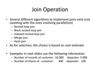
1. Join Operation
• Several different algorithms to implement joins exist (not
counting with the ones involving parallelism)
– Nested-loop join
– Block nested-loop join
– Indexed nested-loop join
– Merge-join
– Hash-join
• As for selection, the choice is based on cost estimate
• Examples in next slides use the following information
– Number of records of customer: 10.000 depositor: 5.000
– Number of blocks of customer: 400 depositor: 100

2. Nested-Loop Join
• The simplest join algorithms, that can be used independently of
everything (like the linear search for selection)
• To compute the theta join r  s
for each tuple tr in r do begin
for each tuple ts in s do begin
test pair (tr,ts) to see if they satisfy the join condition 
if they do, add tr • ts to the result.
end
end
• r is called the outer relation and s the inner relation of the join.
• Quite expensive in general, since it requires to examine every
pair of tuples in the two relations.

3. Nested-Loop Join (Cont.)
• In the worst case, if there is enough memory only to hold
one block of each relation, the estimated cost is
nr  bs + br
block transfers, plus
nr + br
seeks
• If the smaller relation fits entirely in memory, use that as
the inner relation.
– Reduces cost to br + bs block transfers and 2 seeks
• In general, it is much better to have the smaller relation
as the outer relation
– The number of block transfers is multiplied by the number of
blocks of the inner relation
• However, if the smaller relation is small enough to fit in
memory, one should use it as the inner relation!
• The choice of the inner and outer relation strongly
depends on the estimate of the size of each relation

4. Nested-Loop Join Cost in Example
• Assuming worst case memory availability cost estimate is
– with depositor as outer relation:
• 5.000  400 + 100 = 2.000.100 block transfers,
• 5.000 + 100 = 5100 seeks
– with customer as the outer relation
• 10.000  100 + 400 = 1.000.400 block transfers, 10.400 seeks
• If smaller relation (depositor) fits entirely in memory, the
cost estimate will be 500 block transfers and 2 seeks
• Instead of iterating over records, one could iterate over
blocks. This way, instead of nr  bs + br we would have br  bs + br
block transfers
• This is the basis of the block nested-loops algorithm
(next slide).

5. Block Nested-Loop Join
• Variant of nested-loop join in which every block
of inner relation is paired with every block of
outer relation.
for each block Br of r do begin
for each block Bs of s do begin
for each tuple tr in Br do begin
for each tuple ts in Bs do begin
Check if (tr,ts) satisfy the join
condition
if they do, add tr • ts to the result.
end
end
end
end

6. Block Nested-Loop Join Cost
• Worst case estimate: br  bs + br block transfers and 2
* br seeks
– Each block in the inner relation s is read once for each
block in the outer relation (instead of once for each tuple
in the outer relation
• Best case (when smaller relation fits into memory): br +
bs block transfers plus 2 seeks.
• Some improvements to nested loop and block nested
loop algorithms can be made:
– Scan inner loop forward and backward alternately, to make
use of the blocks remaining in buffer (with LRU
replacement)
– Use index on inner relation if available to faster get the
tuples which match the tuple of the outer relation at hands

7. Indexed Nested-Loop Join
• Index lookups can replace file scans if
– join is an equi-join or natural join and
– an index is available on the inner relation’s join attribute
• In some cases, it pays to construct an index just to compute a join.
• For each tuple tr in the outer relation r, use the index on s to look
up tuples in s that satisfy the join condition with tuple tr.
• Worst case: buffer has space for only one page of r, and, for each
tuple in r, we perform an index lookup on s.
• Cost of the join: br (tT + tS) + nr  c
– Where c is the cost of traversing index and fetching all matching s
tuples for one tuple or r
– c can be estimated as cost of a single selection on s using the join
condition (usually quite low, when compared to the join)
• If indices are available on join attributes of both r and s,
use the relation with fewer tuples as the outer relation.

8. Example of Nested-Loop Join Costs
• Compute depositor customer, with depositor as the outer
relation.
• Let customer have a primary B+-tree index on the join attribute
customer-name, which contains 20 entries in each index node.
• Since customer has 10.000 tuples, the height of the tree is 4,
and one more access is needed to find the actual data
• depositor has 5.000 tuples
• For nested loop: 2.000.100 block transfers and 5.100 seeks
• Cost of block nested loops join
– 400*100 + 100 = 40.100 block transfers + 2 * 100 = 200 seeks
• Cost of indexed nested loops join
– 100 + 5.000 * 5 = 25.100 block transfers and seeks.
– CPU cost likely to be less than that for block nested loops join
– However in terms of time for transfers and seeks, in this case
using the index doesn’t pay (this is specially so because the
relations are small)

9. Merge-Join
1. Sort both relations on their join attribute (if not already sorted on
the join attributes).
2. Merge the sorted relations to join them
1. Join step is similar to the merge stage of the sort-merge algorithm.
2. Main difference is handling of duplicate values in join attribute —
every pair with same value on join attribute must be matched
3. Detailed algorithm may be found in the book

10. Merge-Join (Cont.)
• Can be used only for equi-joins and natural joins
• Each block needs to be read only once (assuming that all tuples
for any given value of the join attributes fit in memory)
• Thus the cost of merge join is (where bb is the number of blocks
in allocated in memory):
br + bs block transfers + br / bb + bs / bb seeks
– + the cost of sorting if relations are unsorted.
• hybrid merge-join: If one relation is sorted, and the other has a
secondary B+-tree index on the join attribute
– Merge the sorted relation with the leaf entries of the B+-tree .
– Sort the result on the addresses of the unsorted relation’s tuples
– Scan the unsorted relation in physical address order and merge with
previous result, to replace addresses by the actual tuples
• Sequential scan more efficient than random lookup

11. Hash-Join
• Also only applicable for equi-joins and natural joins.
• A hash function h is used to partition tuples of both
relations
• h maps JoinAttrs values to {0, 1, ..., n}, where JoinAttrs
denotes the common attributes of r and s used in the
natural join.
– r0, r1, . . ., rn denote partitions of r tuples
• Each tuple tr  r is put in partition ri where i = h(tr [JoinAttrs]).
– s0, s1. . ., sn denotes partitions of s tuples
• Each tuple ts s is put in partition si, where i = h(ts [JoinAttrs]).
• General idea:
– Partition the relations according to this
– Then perform the join on each partition ri and si
• There is no need to compute the join between different
partitions since an r tuple and an s tuple that satisfy the join
condition will have the same value for the join attributes. If that
value is hashed to some value i, the r tuple has to be in ri and
the s tuple in si.

12. Hash-Join (Cont.)

13. Hash-Join Algorithm
1. Partition the relation s using hashing function h.
When partitioning a relation, one block of memory is
reserved as the output buffer for each partition.
2. Partition r similarly.
3. For each i:
(a) Load si into memory and build an in-memory hash
index on it using the join attribute. This hash index uses
a different hash function than the earlier one h.
(b) Read the tuples in ri from the disk one by one. For each
tuple tr locate each matching tuple ts in si using the in-
memory hash index. Output the concatenation of their
attributes.
The hash-join of r and s is computed as follows.
Relation s is called the build input and
r is called the probe input.

14. Hash-Join algorithm (Cont.)
• The number of partitions n for the hash function h is
chosen such that each si should fit in memory.
– Typically n is chosen as bs/M * f where f is a “fudge
factor”, typically around 1.2, to avoid overflows
– The probe relation partitions ri need not fit in memory
• Recursive partitioning required if number of
partitions n is greater than number of pages M of
memory.
– instead of partitioning n ways, use M – 1 partitions for s
– Further partition the M – 1 partitions using a different
hash function
– Use same partitioning method on r
– Rarely required: e.g., recursive partitioning not needed
for relations of 1GB or less with memory size of 2MB, with
block size of 4KB.
• So is not further considered here (see the book for details on
the associated costs)

15. Cost of Hash-Join
• The cost of hash join is
3(br + bs) +4  nh block transfers +
2( br / bb + bs / bb) seeks
• If the entire build input can be kept in main memory no
partitioning is required
– Cost estimate goes down to br + bs.
• For the running example, assume that memory size is 20 blocks
• bdepositor= 100 and bcustomer = 400.
• depositor is to be used as build input. Partition it into five
partitions, each of size 20 blocks. This partitioning can be done
in one pass.
• Similarly, partition customer into five partitions, each of size 80.
This is also done in one pass.
• Therefore total cost, ignoring cost of writing partially filled
blocks:
– 3(100 + 400) = 1.500 block transfers +
2( 100/3 + 400/3) = 336 seeks
• The best we had up to here was 40.100 block transfers plus 200
seeks (for block nested loop) or 25,100 block transfers and
seeks (for index nested loop)

16. Complex Joins
• Join with a conjunctive condition:
r 1  2...   n s
– Either use nested loops/block nested loops, or
– Compute the result of one of the simpler joins r i s
• final result comprises those tuples in the intermediate
result that satisfy the remaining conditions
1  . . .  i –1  i +1  . . .  n
• Join with a disjunctive condition
r 1  2 ...  n s
– Either use nested loops/block nested loops, or
– Compute as the union of the records in individual
joins r  i s:
(r 1 s)  (r 2 s)  . . .  (r n s)