The document discusses correlation and regression analysis. It provides an overview of key concepts like the regression coefficient, correlation coefficient, and fitted line plots. It also describes how to calculate regression using the method of least squares and how to validate factors using tools like t-tests, ANOVA, and regression. An example is shown analyzing the relationship between softening temperature measured at a supplier vs. a customer. The correlation between the two factors is calculated to be 0.834, indicating a strong positive correlation.

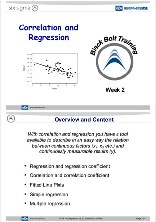
1. C l ti dCorrelation and
RegressionRegression
110
100
90
80
70
60
Output
50403020100
60
50
40
50403020100
Input
Week 2
Knorr-Bremse Group
Overview and Content
With correlation and regression you have a toolg y
available to describe in an easy way the relation
between continuous factors (x1, x2 etc.) and1 2
continuously measurable results (y).
• Regression and regression coefficient
• Correlation and correlation coefficient
• Fitted Line Plots• Fitted Line Plots
• Simple regressionp g
• Multiple regression
Knorr-Bremse Group 07 BB W2 Regression 08, D. Szemkus/H. Winkler Page 2/24

2. Validation of Factors Y = f (x)
Overview about the validation of
single factors to single results
Factor X = Input
Discrete / Attributive Continuous / Variable
single factors to single results
Discrete / Attributive Continuous / Variable
e
ve
Output
Discrete
ttributiv
Chi-Square
Logistic
Regression
tY=O
D
At
s
Resul
tinuous
riable
T - Test
ANOVA ( F - Test) RegressionRegression
Con
Va
( )
Variance Test
eg ess o
Knorr-Bremse Group 07 BB W2 Regression 08, D. Szemkus/H. Winkler Page 3/24
Regression
xbbyˆ 21
+=
y
The fitted, estimated value of the
dependent variable.
yˆ
21
i
y
ei
The zero point shift
The slope of the straight line
1
b
2
b
yˆ The difference between the fitted
(calculated) values and the
observed values
ei
1
b
x
ϕ
observed values
Recieving Ch = 91,4033 + 0,476288 Final check
Regression Plot
i
x x
0
∑ ∑ ∑ ∑−
n n n n
iiii
2
i
yxxyx
b
210
200
h
S = 6,77854 R-Sq = 69,5 % R-Sq(adj) = 67,9 %
( )∑ ∑= =
= = = =
−
= n
1i
2n
1i i
2
i
1i 1i 1i 1i iiiii
1
xxn
yy
b 190
180
RecievingCh
( )∑ ∑
∑ ∑ ∑= = =
−
−
= n 2n
2
n
1i
n
1i
n
1i iiii
2
xxn
yxyxn
b 230220210200190180170
170
160
Final check
Knorr-Bremse Group 07 BB W2 Regression 08, D. Szemkus/H. Winkler Page 4/24
( )∑ ∑= =
−1i 1i ii
xxn Final check

3. Regression
The method of the smallest quadratic deviations has 4 important
properties:p p
• The sum of the residuals values is zero
• The sum of the products of the values of the x variable and
corresponding residuals is equal to zero
• The arithmetic means of the measured Y variable and the
theoretic calculated Y variable (fitted values) are equaltheoretic calculated Y variable (fitted values) are equal
• The regression straight line runs through the “center of gravity” of
th tt l tthe scatter plot
Which statement can we make about the
significance of the relation?
Knorr-Bremse Group 07 BB W2 Regression 08, D. Szemkus/H. Winkler Page 5/24
g
Regression Example
An example: The results shows the soften temperature measured during the final
check at the supplier and the receiving check at the customer. The values of two
different plastic types are included in the two columns
Stat
different plastic types are included in the two columns
File:
Soften temperature.mtw
>Regression
>Fitted Line Plot… Fitted Line Plot
Recieving Check = 91 40 + 0 4763 Final check
p
210
200
S 6,77854
R-Sq 69,5%
R-Sq(adj) 67,9%
Recieving Check = 91,40 + 0,4763 Final check
Final check Recieving Check Material
190
ingCheck
Final check Recieving Check Material
168 162,5 1
209 187,5 2
177,5 183,5 1
222,5 192,5 2
180
170
Recievi
, ,
182,5 187,5 1
227,5 197,5 2
197,5 197,5 2
202,5 182,5 2
240230220210200190180170160
160
Final check
173 177,5 1
214,5 192,5 2
182,5 182,5 1
222,5 202,5 2
Knorr-Bremse Group 07 BB W2 Regression 08, D. Szemkus/H. Winkler Page 6/24
Final check
197,5 187,5 2

4. Regression
Also in the session window we get the regression equation
I dditi th i ifi i l l t d b th i l iIn addition, the significance is calculated by the variance analysis
Regression Analysis: Recieving Check versus Final check
The regression equation isThe regression equation is
Recieving Check = 91,4 + 0,476 Final check
S = 6,77854 R-Sq = 69,5% R-Sq(adj) = 67,9%
Analysis of VarianceAnalysis of Variance
Source DF SS MS F P
Regression 1 1989,0 1989,0 43,29 0,000
Residual Error 19 873,0 45,9
Total 20 2862,0
Knorr-Bremse Group 07 BB W2 Regression 08, D. Szemkus/H. Winkler Page 7/24
R2 and R2 adj.: Practical Significance
• R² is a method within the statistics, to show the practical significance of
an effect.
695,0
2862
1989Re2
===
Total
gression
SS
SS
R
Explained variation (SS Regression) divided by the total
variation (SS Total). Approximately 70% of the
variation is explained by the samples.
• R² adj. is a similar method to explain the practical significance of an
ff t It i h l f l if l f t i d l E R2 dj teffect. It is helpful, if we use several factors in a model. E.g. R2 adj. gets
smaller, if an additional factor is added in the model, because every
reduction of SS error can be balanced by the loss of degrees of freedom.reduction of SS error can be balanced by the loss of degrees of freedom.
The values for R² adj. are always a little bit smaller than for R².
9545MS
68,0
20
2862
95,45
112
=−=−=
Total
Total
Error
DF
SS
MS
adjR
Total
• S is the pooled standard deviation (averaged within group variation) The
square root of S is the MS Error
Knorr-Bremse Group 07 BB W2 Regression 08, D. Szemkus/H. Winkler Page 8/24
square root of S is the MS Error.

5. Correlation
• Correlation is a measure for the strength of a interaction between two
quantitative variables (e.g. measurement at supplier and customer).quantitative variables (e.g. measurement at supplier and customer).
• Correlation measures the degree of linearity between two variables.
• The value of the correlation coefficient r ranges between -1 and 1
• Rule: A correlation > 0 80 or < 0 80 is significant a• Rule: A correlation > 0,80 or < -0,80 is significant, a
correlation between -0,80 and 0,80 is not significant.
L t h l k t th l ft t t• Lets have look at the example soften temperature. Covariance
(x x) (y y)i i
n
− −
∑
1x x y yi
n
i− −
∑
1
( )( ) r
n -1
xy
xi=1
= ∑ s s y
r
n -1
x x y y
xy
i
xi=1
i
y
= ∑
1
s s( )( ) =
Knorr-Bremse Group 07 BB W2 Regression 08, D. Szemkus/H. Winkler Page 9/24
The Calculation
The calculation of the covariance and correlation coefficient
Final Insp Incoming Insp Yi - Ymean Xi - X mean Covariance r
168 162 5 25 33 8 844 3 37168 162,5 -25 -33,8 844 3,37
209 187,5 0 7,2 0 0,00
177,5 183,5 -4 -24,3 97 0,39
222,5 192,5 5 20,7 104 0,41
182,5 187,5 0 -19,3 0 0,00
227,5 197,5 10 25,7 257 1,03
197,5 197,5 10 -4,3 -43 -0,17
202,5 182,5 -5 0,7 -4 -0,01
173 177,5 -10 -28,8 288 1,15
214,5 192,5 5 12,7 64 0,25
182,5 182,5 -5 -19,3 96 0,38
222,5 202,5 15 20,7 311 1,24, , , ,
197,5 187,5 0 -4,3 0 0,00
232,5 202,5 15 30,7 461 1,84
173 167,5 -20 -28,8 575 2,30
208 5 197 5 10 6 7 67 0 27208,5 197,5 10 6,7 67 0,27
182,5 172,5 -15 -19,3 289 1,15
222,5 197,5 10 20,7 207 0,83
194 176,5 -11 -7,8 85 0,34
229 5 207 5 20 27 7 555 2 21229,5 207,5 20 27,7 555 2,21
217,5 182,5 -5 15,7 -79 -0,31
Mean 201,8 187,5 4176 16,67
Stdev 20,9 12,0 Covariance 208,8 0,83 r
Knorr-Bremse Group 07 BB W2 Regression 08, D. Szemkus/H. Winkler Page 10/24

6. Calculation in Minitab
Stat
>Basic Statistics File:
Soften temperature mtw
Correlation of the final check and receiving check r = 0 834
>Correlation…
Soften temperature.mtw
Correlation of the final check and receiving check r 0,834
² 0 695r² = 0,695
r = 0,834
Knorr-Bremse Group 07 BB W2 Regression 08, D. Szemkus/H. Winkler Page 11/24
Exercise: Simulated Data
• We generate two columns with 50 random
numbers each and correlate these values.
Calc
>Random Data
– Mean: 100
– Standard deviation: 10
>Random Data
>Normal…
– Standard deviation: 10
Which value do we expect for the correlation? Stat• Which value do we expect for the correlation? Stat
>Basic Statistics
>Correlation…
• Investigate the correlation.
– Does the correlation correspond to our
expectations?
Stat
>Regression
• Use the Fitted Line Plot function and
investigate r².
>Fitted Line Plot…
Knorr-Bremse Group 07 BB W2 Regression 08, D. Szemkus/H. Winkler Page 12/24

7. Examples for Positive Correlation
76
74
S 0,838232
R-Sq 93,2%
R-Sq(adj) 93,1%
Strong Positive Correlation
Output = 57,39 + 0,1732 Input
74
72
70
68
Output
R Sq(adj) 93,1%
85
80
Moderate Positive Correlation
Output = 53,28 + 0,2109 Input
100908070605040
66
64
62
80
75
70
65
Output
Input
90
Weak Positive Correlation
Output = 58,31 + 0,1635 Input
100908070605040
65
60
55
S 5,18519
R-Sq 34,6%
R-Sq(adj) 33,5%
80
70
60
Output
Input
100908070605040
50
40
Input
S 10,4391
R-Sq 7,3%
R-Sq(adj) 5,7%
Knorr-Bremse Group 07 BB W2 Regression 08, D. Szemkus/H. Winkler Page 13/24
Input
Examples for Negative Correlation
52,5 S 1,16327
R-Sq 88,3%
R S ( dj) 88 1%
Strong Negative Correlation
Output = 56,48 - 0,1786 Input
50,0
47,5
45,0
Output
R-Sq(adj) 88,1%
100908070605040
42,5
40,0
65
60
S 4,44849
R-Sq 39,3%
R-Sq(adj) 38,3%
Moderate Negative Correlation
Output = 58,46 - 0,1999 Input
100908070605040
Input
60
55
50
45
Output
100908070605040
45
40
35 70
60
S 8,74951
R-Sq 12,1%
R-Sq(adj) 10,6%
Weak Negative Correlation
Output = 57,34 - 0,1813 Input
Input 60
50
40
Output
100908070605040
30
20
Input
Knorr-Bremse Group 07 BB W2 Regression 08, D. Szemkus/H. Winkler Page 14/24
Input

8. How large should the Coefficient „r“ be?
Compare your correlation value with
the value in the table according to your
Sample size d.f. Significance level
n n-2 0,05 0,025 0,01 0,005
3 1 0,9877 0,9969 0,9995 0,9999
4 2 0,9000 0,9500 0,9800 0,9900
5 3 0 8054 0 8783 0 9343 0 9587the value in the table according to your
sample size. Is the value larger than
noted in the table the correlation is
5 3 0,8054 0,8783 0,9343 0,9587
6 4 0,7293 0,8114 0,8822 0,9172
7 5 0,6694 0,7545 0,8329 0,8745
8 6 0,6215 0,7067 0,7887 0,8343
9 7 0,5822 0,6664 0,7498 0,7977
“important” or statistically significant. 10 8 0,5494 0,6319 0,7155 0,7646
11 9 0,5214 0,6021 0,6851 0,7348
12 10 0,4973 0,5760 0,6581 0,7079
13 11 0,4762 0,5529 0,6339 0,6835
14 12 0 4575 0 5324 0 6120 0 66142
t 14 12 0,4575 0,5324 0,6120 0,6614
15 13 0,4409 0,5140 0,5923 0,6411
16 14 0,4259 0,4973 0,5742 0,6226
17 15 0,4124 0,4821 0,5577 0,6055
18 16 0,4000 0,4683 0,5425 0,5897
19 17 0 3887 0 4555 0 5285 0 5751
2
2
2
or
tn
t
r +−
=α α
α
19 17 0,3887 0,4555 0,5285 0,5751
20 18 0,3783 0,4438 0,5155 0,5614
21 19 0,3687 0,4329 0,5034 0,5487
22 20 0,3598 0,4227 0,4921 0,5368
27 25 0,3233 0,3809 0,4451 0,48692
1
2
or
r
rn
t ⋅−
=α
32 30 0,2960 0,3494 0,4093 0,4487
37 35 0,2746 0,3246 0,3810 0,4182
42 40 0,2573 0,3044 0,3578 0,3932
47 45 0,2429 0,2876 0,3384 0,3721
52 50 0,2306 0,2732 0,3218 0,3542
1 r−α
Attention! Due to big sample sizes 52 50 0,2306 0,2732 0,3218 0,3542
62 60 0,2108 0,2500 0,2948 0,3248
72 70 0,1954 0,2319 0,2737 0,3017
82 80 0,1829 0,2172 0,2565 0,2830
92 90 0,1726 0,2050 0,2422 0,2673
102 100 0 1638 0 1946 0 2301 0 2540
also r- values <0,8 are significant.
Be aware here, the risk of
misinterpretation is relatively high
Knorr-Bremse Group 07 BB W2 Regression 08, D. Szemkus/H. Winkler Page 15/24
102 100 0,1638 0,1946 0,2301 0,2540misinterpretation is relatively high.
Avoid Quick Conclusions
If y and x1 correlate well that does not necessarily mean that a
variation of x will cause a variation of y.
A third variable could be in the background which is responsible
for the change of the x as well of the y.g y
An example from production shows a strong negative correlation
between the pressure (x) and yield (y) in a reactor butbetween the pressure (x) and yield (y) in a reactor, but…
There are contaminations (x2), which are not measured and vary
f l t lfrom process cycle to process cycle.
– Contamination is causing foaming
– Contamination is causing poor yield
Th i d t d th f b ild– The pressure is used to reduce the foam build up
– The pressure is a reaction on the foam build up and has no effect
th i ld
Knorr-Bremse Group 07 BB W2 Regression 08, D. Szemkus/H. Winkler Page 16/24
on the yield

9. Another Example
• Open the file:Open the file:
MYSTERY.MTWMYSTERY.MTW
• Calculate the correlation
10
Scatterplot of Output vs Input
• Calculate the correlation.
• Is there a correlation
put
8
6
4
between the two variables?
• Create a plot for both
Outp
2
0
-2
p
variables.
• What is your conclusion for
Input
210-1-2-3
-4
What is your conclusion for
the correlation?
Knorr-Bremse Group 07 BB W2 Regression 08, D. Szemkus/H. Winkler Page 17/24
Simple Regression
Correlation describes the linear dependence of two variables
regression defines this relation more detailedregression defines this relation more detailed.
Regression leads to an equation, which uses one (or more)
variables to explain the variation of the output variable.
St t > R i > R iStat > Regression > Regression…
Performs simple and multiple regression
Stat > Regression > Fitted Line Plot…
Scatter Plot Fitted Line equation and r²Scatter Plot, Fitted Line, equation and r
Stat > Regression > Residuals Plots…
Stores the residuals of the “regression" or "Fitted line plot"
Proofs basic assumptions about the behavior of the residuals
Knorr-Bremse Group 07 BB W2 Regression 08, D. Szemkus/H. Winkler Page 18/24

10. Summary
C l ti i f l t l t d ib d d i• Correlation is a useful tool to describe dependencies
during many improvement activities.
• Correlation is the measure of the linear relation
between two quantitative variables.
• Avoid too fast conclusion for causes.
C f• Correlation is the basis for the regression method.
• Regression describes the relation of the variablesRegression describes the relation of the variables
more detailed and shows a equation model.
Knorr-Bremse Group 07 BB W2 Regression 08, D. Szemkus/H. Winkler Page 19/24
AppendixAppendix
Further ExamplesFurther Examples
Knorr-Bremse Group 07 BB W2 Regression 08, D. Szemkus/H. Winkler Page 20/24

11. Example; Retailer Sales and Cost of Production
Area Frequency Sales
310 10240 2930
980 7510 5270
File: Sales.mtw
A t il h i t t i ti t th1210 10810 6850
1290 9890 7010
1120 13720 7020
1490 13920 8350
A retailer chain wants to investigate the
sales dependence of shop location(Area)
and the passerby frequency.1490 13920 8350
780 8540 4330
940 12360 5770
1290 12270 7680
p y q y
What kind of relations you can describe?
1290 12270 7680
480 11010 3160
240 8250 1520
550 9310 3150
Units Cost
3200 32200
4100 327004100 32700
10700 70100
8700 48200File Cost mtw
6500 38600
9400 55400
11200 77200
File. Cost.mtw
The table shows the production fix costs
f 10 11200 77200
1400 24300
6000 37500
and the number of units over 10 month.
Determine the favorable production size.
Knorr-Bremse Group 07 BB W2 Regression 08, D. Szemkus/H. Winkler Page 21/24
4200 34000
p
Example; Salary
File: Salery.mtwy
Evaluate the factors, which of them has the
strongest effect on salary?strongest effect on salary?
Salary Year in the job Company years Education Age Pers. No. Sex Sex Group
38985 18 7 9 52 412 M 0
28938 12 5 4 39 517 F 1
32920 15 3 9 45 458 F 1
29548 5 6 1 30 604 M 0
31138 11 11 6 46 562 F 1
24749 6 2 0 26 598 F 124749 6 2 0 26 598 F 1
41889 22 16 7 63 351 M 0
31528 3 11 3 35 674 M 0
38791 21 4 5 48 356 M 0
39828 18 6 5 47 415 F 139828 18 6 5 47 415 F 1
Knorr-Bremse Group 07 BB W2 Regression 08, D. Szemkus/H. Winkler Page 22/24

12. The Mystery Example
10
8
S 1,69190
R-Sq 6,4%
R Sq(adj) 5 4%
Fitted Line Plot
Output = 1,145 - 0,4340 Input
If we use Stat > Regression > Fitted
put
8
6
4
R-Sq(adj) 5,4%If we use Stat > Regression > Fitted
Line Plot > Linear we get…
Outp
2
0
Input
210-1-2-3
-2
-4
12 Regression
Fitted Line Plot
Output = 0,1401 + 0,0413 Input
+ 1,025 Input**2
10
8
6
S 1,02499
R-Sq 66,0%
R-Sq(adj) 65,3%
95% CI
Output
4
2
0
If we use Stat > Regression > Fitted
210-1-2-3
0
-2
-4
Line Plot > quadratic Regression we
get a strong correlation.
Knorr-Bremse Group 07 BB W2 Regression 08, D. Szemkus/H. Winkler Page 23/24
Input
Example; Retailer Sales
Diagnosis at regression
Stat
9000 S 408,182
R-Sq 96,9%
Fitted Line Plot
Sales = 605,7 + 5,222 Area
>Regression
>Residual Plot…
s
8000
7000
6000
R-Sq(adj) 96,6%
Evaluation like at ANOVA
Sales
5000
4000
3000
Area
1600140012001000800600400200
2000
1000
99
90
l
500
Normal Probability Plot of the Residuals Residuals Versus the Fitted Values
Residual Plots for Sales
Mi it b d th id l d
Percent
10005000-500-1000
50
10
1
Residual
8000600040002000
0
-500
Minitab needs the residuals and
the fits in one column. Storage
of residuals and fits is possible
Residual
100050005001000
Fitted Value
8000600040002000
4
3
500
Histogram of the Residuals Residuals Versus the Order of the Data
during every evaluation.
Frequency
3
2
1
0
Residual
0
-500
Knorr-Bremse Group 07 BB W2 Regression 08, D. Szemkus/H. Winkler Page 24/24
Residual
7505002500-250-500
0
Observation Order
121110987654321