Download to read offline


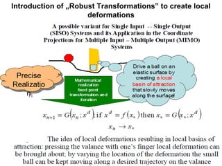
![A possibility is the utilization of the strongly saturated nature
of sigmoid functions with σ(0)=0 for SISO systems
G ( r; r d
) = ( r + K )[1 + B tanh ( A[ f ( r ) − r ]) ] − K d
BAf ′( r )
G' = ( r + K ) + [1 + B tanh ( A[ f ( r ) − r d ] ) ]
cosh 2 ( A[ f ( r ) − r d ] )
False fixed point: G(-K;rd)=-K Good fixed point: if f(r*)=rd then G(r*;rd)=r*
The derivative easily can be made small enough in the fixed point
to obtain convergent iteration:
G ' ( r∗ ) = ( r∗ + K ) BAf ′( r∗ ) + 1
For this purpose the manipulation of three adaptive control
parameters (A,B,K) is needed. The design of the control
parameters can be done in a few simple steps via simulation:](https://image.slidesharecdn.com/itsworldcongressvienna2012october-121021145255-phpapp02/85/ITS-World-Congress-Vienna-Oct-2012-10-320.jpg)


![Non-adaptive tracking of ρ3 [vehicle/km] vs. time [h] (ξ=0)
v1, v2, v3 versus time [h]
Nominal Simulated 120
118
[km/h]
116
114
112
110
108
106
104
1234
0.0 0.5 1.0 1.5 2.0
rho1, rho2, rho3, rho4 versus time [h]
18
[vehicle/km]
16
14
12
10
8
6
4
2
0
0.0 0.5 1.0 1.5 2.0
r2 versus time [h]
1600
[vehicle/h]
1400
1200
1000
800
600
400
200
0
0.0 0.5 1.0 1.5 2.0
Sampling time: 20 s, K= −104, B=1, A=0.25×10⁻⁴, Ks=10−6
This chart reveals the effects of
the modeling errors](https://image.slidesharecdn.com/itsworldcongressvienna2012october-121021145255-phpapp02/85/ITS-World-Congress-Vienna-Oct-2012-15-320.jpg)
![Adaptive tracking of ρ3 [vehicle/km] vs. time [h] (ξ=0)
Nominal Simulated
1234
Sampling time: 20 s, K= −104, B=1, A=0.25×10⁻⁴, Ks=10−6
This chart reveals the effects of
adaptivity](https://image.slidesharecdn.com/itsworldcongressvienna2012october-121021145255-phpapp02/85/ITS-World-Congress-Vienna-Oct-2012-16-320.jpg)
![Tracking of Ef [vehicle×km2/h3] vs. time [h] (ξ=1)
Nominal Tracking of E.F. vs. time
1.6e+007
1.5e+007
1.4e+007 Simulated Nominal
1.3e+007
1.2e+007
1.1e+007 Simulated
1.0e+007
9.0e+006
0.0 0.2 0.4 0.6 0.8 1.0 1.2 1.4 1.6
Tracking error vs. time
4e+006
3e+006
2e+006
1e+006 Non-adaptive
0e+000
-1e+006
Adaptive
-2e+006
-3e+006
0.0 0.2 0.4 0.6 0.8 1.0 1.2 1.4 1.6
q0 vs. time
450
350
250
150
0.0 0.2 0.4 0.6 0.8 1.0 1.2 1.4 1.6
Sampling time: 20 s, K= −104, B=1, A=0.25×10⁻⁴, Ks=10−6](https://image.slidesharecdn.com/itsworldcongressvienna2012october-121021145255-phpapp02/85/ITS-World-Congress-Vienna-Oct-2012-17-320.jpg)
![Adaptive tracking of fcompr [vehicle/km] vs. time [h] (ξ=0)
Simulated
Required: adaptively deformed
Desired
Sampling time: 20 s, K= −104, B=1, A=0.25×10⁻⁴, Ks=10−6](https://image.slidesharecdn.com/itsworldcongressvienna2012october-121021145255-phpapp02/85/ITS-World-Congress-Vienna-Oct-2012-18-320.jpg)
![Adaptive tracking of fcompr [vehicle/km] vs. time [h] (ξ=0.4)
f o p d s r d s m l t d r q i e v r u t m [ ]
c m r e i e , i u a e , e u r d e s s i e h
18
Desired
16 Simulated
v h c e k ]
[ e i l / m
14
12
10
8
Required: adaptively deformed
0 0
. 0 5
. 1 0
. 1 5
. 2 0
.
Sampling time: 20 s, K= −104, B=1, A=0.25×10⁻⁴, Ks=10−6](https://image.slidesharecdn.com/itsworldcongressvienna2012october-121021145255-phpapp02/85/ITS-World-Congress-Vienna-Oct-2012-19-320.jpg)


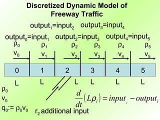
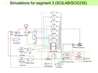
This document discusses the development of an iterative adaptive control system for managing freeway traffic emissions, utilizing simplified mathematical methodologies and macroscopic dynamic models. It highlights the challenges of modeling uncertainties and the need for adaptive control strategies amidst non-linear dynamics. The findings suggest that basic computational tools can effectively implement robust linear transformations to achieve satisfactory traffic management outcomes.