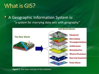
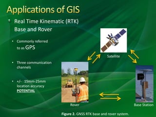
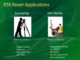
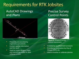
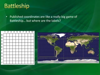
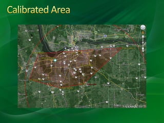
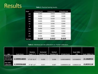
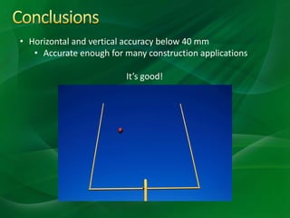
Group 01CW
Brandon Nussey, Bryan Dewar,
Ronald Darraugh, & Simon Sweeney
• Introduction
• What is GIS?
• GIS Applications
• RTK Rovers and Requirements
• Localizing a jobsite
• Approach
• Results
• Conclusions
• Recommendations
• Acknowledgements
• Questions?
• Setting up GPS jobsites is time consuming
• Using an RTK GPS base and rover, a form of GIS
technology; we created a digital file and calibrated a
major portion of Ottawa’s geography
• By doing this, we’ve eliminated the need to calibrate
individual jobsites for each new project
A Geographic Information System is:
“a system for marrying data sets with geography”
Figure 1. The basic concept of GIS software.
Real Time Kinematic (RTK)
Base and Rover
Satellite
Rover
• Commonly referred
to as GPS
• Three communication
channels
• +/- 15mm-25mm
location accuracy
POTENTIAL
Base Station
Figure 2. GNSS RTK base and rover system.
Surveying
Figure 3. A surveyor. Figure 4. A mobile rover.
- Feature Layout
- Stake out
- Real-time “cuts”
and “fills”
- Topographic surveys
or “TOPO’s”
- “As-builts”
- On-site volume and
area calculations
Site Works
AutoCAD Drawings
and Plans
Precise Survey
Control Points
Figure 5. A typical survey
control monument.Prepared and provided by
engineers, consultants
Contain spatial information
and line work
Used to create designs, maps,
and everything visible on data
collector screen
Installed by qualified land surveyors
Provided to contractors by City of
Ottawa, MTO, etc.
Used to localize or calibrate jobsites
• Published coordinates are like a really big game of
Battleship… but where are the labels?
• 3-dimensional, curved surface of
the Earth is being represented on
flat, 2-dimensional plans
• Distortion is INVEVITABLE
• Shapes and sizes can become
misrepresented
Figure 6. A ripped orange peel representing
data transfer distortion.
• Control points “pin” the digital plans, to
the Earth’s surface
• “Iron out the wrinkles”
• Done through CALIBRATION
Figure 9. Range of base station.
• Find reliable network of control points
• Measure in control points
• Testing: practical and theoretical
Point ∆ Northing (m) ∆ Easting (m) ∆ Elevation (m)
168 0.042 0.013 0.026
142 0.050 0.009 0.038
143 0.032 0.020 0.010
145 0.035 0.002 0.010
73 0.055 0.036 0.049
3 0.014 0.021 0.014
170 0.050 0.003 0.011
171 0.042 0.005 0.012
59 0.037 0.005 0.008
173 0.036 0.008 0.014
Average= 0.039 0.012 0.019
Table 1. Practical testing results.
Job Scale Factor
Rotation
Angle (°,',")
Horizontal
Residual (m)
Vertical
Residual (m) ∆ Scale Factor
∆ per 100m
(m) ∆ per 1000m (m)
Individual
site average 0.999914835 0° 33' 52.3" 0.020 0.036 0.0001068955 0.01068954 0.1068954
City-wide
calibration 0.999996488 0° 00' 1.0" 0.017 0.007 0.0000035118 0.00035118 0.0035118
Table 2. Individual job site calibrations vs. master calibration.
• Horizontal and vertical accuracy below 40 mm
• Accurate enough for many construction applications
It’s good!
Give it a try!
Waiting for issued control points = time consuming
Searching for control points = time consuming
Calibrating individual sites = time consuming
TIME = MONEY
Francesco Tangorra
Patrick Dawson
Marieke Kalkhove
Federico Fernandez
TJ Hendriks
Pierre Boivin
Bob Lefebvre
Jacques Perriard
Jean-Francois Goulet
Justin Vanhecke
Investigating GIS Technologies - Group 01CW Final Presentation

Investigating GIS Technologies - Group 01CW Final Presentation

  • 1.
    Group 01CW Brandon Nussey,Bryan Dewar, Ronald Darraugh, & Simon Sweeney
  • 2.
    • Introduction • Whatis GIS? • GIS Applications • RTK Rovers and Requirements • Localizing a jobsite • Approach • Results • Conclusions • Recommendations • Acknowledgements • Questions?
  • 3.
    • Setting upGPS jobsites is time consuming • Using an RTK GPS base and rover, a form of GIS technology; we created a digital file and calibrated a major portion of Ottawa’s geography • By doing this, we’ve eliminated the need to calibrate individual jobsites for each new project
  • 4.
    A Geographic InformationSystem is: “a system for marrying data sets with geography” Figure 1. The basic concept of GIS software.
  • 5.
    Real Time Kinematic(RTK) Base and Rover Satellite Rover • Commonly referred to as GPS • Three communication channels • +/- 15mm-25mm location accuracy POTENTIAL Base Station Figure 2. GNSS RTK base and rover system.
  • 6.
    Surveying Figure 3. Asurveyor. Figure 4. A mobile rover. - Feature Layout - Stake out - Real-time “cuts” and “fills” - Topographic surveys or “TOPO’s” - “As-builts” - On-site volume and area calculations Site Works
  • 7.
    AutoCAD Drawings and Plans PreciseSurvey Control Points Figure 5. A typical survey control monument.Prepared and provided by engineers, consultants Contain spatial information and line work Used to create designs, maps, and everything visible on data collector screen Installed by qualified land surveyors Provided to contractors by City of Ottawa, MTO, etc. Used to localize or calibrate jobsites
  • 8.
    • Published coordinatesare like a really big game of Battleship… but where are the labels?
  • 9.
    • 3-dimensional, curvedsurface of the Earth is being represented on flat, 2-dimensional plans • Distortion is INVEVITABLE • Shapes and sizes can become misrepresented Figure 6. A ripped orange peel representing data transfer distortion. • Control points “pin” the digital plans, to the Earth’s surface • “Iron out the wrinkles” • Done through CALIBRATION
  • 11.
    Figure 9. Rangeof base station.
  • 12.
    • Find reliablenetwork of control points • Measure in control points • Testing: practical and theoretical
  • 14.
    Point ∆ Northing(m) ∆ Easting (m) ∆ Elevation (m) 168 0.042 0.013 0.026 142 0.050 0.009 0.038 143 0.032 0.020 0.010 145 0.035 0.002 0.010 73 0.055 0.036 0.049 3 0.014 0.021 0.014 170 0.050 0.003 0.011 171 0.042 0.005 0.012 59 0.037 0.005 0.008 173 0.036 0.008 0.014 Average= 0.039 0.012 0.019 Table 1. Practical testing results. Job Scale Factor Rotation Angle (°,',") Horizontal Residual (m) Vertical Residual (m) ∆ Scale Factor ∆ per 100m (m) ∆ per 1000m (m) Individual site average 0.999914835 0° 33' 52.3" 0.020 0.036 0.0001068955 0.01068954 0.1068954 City-wide calibration 0.999996488 0° 00' 1.0" 0.017 0.007 0.0000035118 0.00035118 0.0035118 Table 2. Individual job site calibrations vs. master calibration.
  • 15.
    • Horizontal andvertical accuracy below 40 mm • Accurate enough for many construction applications It’s good!
  • 16.
    Give it atry! Waiting for issued control points = time consuming Searching for control points = time consuming Calibrating individual sites = time consuming TIME = MONEY
  • 17.
    Francesco Tangorra Patrick Dawson MariekeKalkhove Federico Fernandez TJ Hendriks Pierre Boivin Bob Lefebvre Jacques Perriard Jean-Francois Goulet Justin Vanhecke