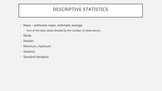
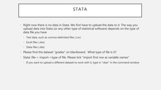
SlideShare a Scribd company logo
1 of 28
INTRODUCTION
Review of Statistics. Stata and Excel introduction
DESCRIPTIVE STATISTICS
ā€¢ Mean ā€“ arithmetic mean, arithmetic average.
ā€¢ Sum of the data values divided by the number of observations
ā€¢ Mode
ā€¢ Median
ā€¢ Minimum, maximum
ā€¢ Variance
ā€¢ Standard deviation
MEAN
ā€¢ Mean - arithmetic mean, arithmetic average. Sum of the data values divided by the
number of observations
ā€¢ Example: Calculate the mean for the hypothetical data for shipments of peanuts from a
U.S. exporter to five Canadian cities
ā€¢ Montreal ā€“ 640,000 pounds
ā€¢ Ottawa ā€“ 15,000 pounds
ā€¢ Toronto ā€“ 285,000 pounds
ā€¢ Vancouver ā€“ 228,000 pounds
ā€¢ Winnipeg ā€“ 45,000 pounds
ā€¢ Notes: Ī£ means sum, unit of observation here is a Canadian city
MEAN CONTā€™D
ā€¢ In excel:
ā€¢ Click on fx and find the function name or type in
ā€¢ =average(range of data)
ā€¢ In Stata:
ā€¢ Import data by clicking on ā€œfileā€ (upper left corner) -> ā€œimportā€ ->pick the format of the file->
find it by clicking ā€browseā€-> tick the box ā€œimport first row as variable namesā€
ā€¢ Mean(peanuts)
STATA
ā€¢ Stata is a powerful tool for researchers and applied economists.
ā€¢ Infinitely extensible, gives users the same development tools used by the companyā€™s professional
programmers
ā€¢ Google is your best friend
ā€¢ Stata has a few windows:
ā€¢ bottom middle is the command window ā€“ this is where you type in the commands;
ā€¢ top middle ā€“ the commands that you submitted appear and so does the output;
ā€¢ left ā€“ all of the commands you have run;
ā€¢ right ā€“ all of the variables you have in your dataset
ā€¢ To view your dataset you can click on ā€œdata editorā€ or ā€œdata browserā€
STATA
ā€¢ Right now there is no data in Stata. We first have to upload the data to it. The way you
upload data into Stata (or any other type of statistical software) depends on the type of
data file you have
ā€¢ Text data, such as comma-delimited files (.csv)
ā€¢ Excel files (.xlsx)
ā€¢ Stata files (.dta)
ā€¢ Please find the dataset ā€œgradesā€ on blackboard. What type of file is it?
ā€¢ Stata: file-> import->type of file. Please tick ā€œimport first row as variable namesā€
ā€¢ If you want to upload a different dataset to work with it, type in ā€œclearā€ in the command window
STATA LOGS AND DO-FILES
ā€¢ log ā€“ records your work in Stata, start before you do anything else!
ā€¢ .do file ā€“ lets you record a series of commands
ā€¢ Try to make your own log and .do file
ā€¢ Click on ā€œlogā€ -> ā€œbeginā€ ->give it a name ->save in the location convenient for you (this starts a
log, when you exit Stata the log will automatically save).
ā€¢ Click on ā€œdo-file editorā€ start typing up commands. You would save it like any other document
(ā€saveā€ -> give it a name, save in a convenient location).
ā€¢ To run the commands in the do-file simply click ā€runā€ at the top of the do-file
EXAMPLE
ā€¢ Calculate mean for the student grades in excel and in Stata
ā€¢ You will find the data set ā€œgradesā€ on blackboard
ā€¢ Make sure your work in Stata is recorded in a log
ā€¢ What is the unit of observation in the dataset (i.e. whose grades are these)?
ā€¢ How many observations are there?
ā€¢ What is the average grade in that class?
SMALLEST AND LARGEST OBSERVATION
ā€¢ You might be wondering if anyone got 100 in the class, or what the highest grade in the class
was and possibly the lowest.
ā€¢ We can do so by looking at the data, by sorting data, and by using minimum and maximum
functions in Excel and Stata
ā€¢ To sort data:
ā€¢ In Excel: highlight the data you want to sort, ā€œdataā€ -> ā€œsortā€
ā€¢ In Stata: sort ā€™variablenameā€™
ā€¢ gsort +ā€™variablenameā€™ or ā€“ā€™variablenameā€™
ā€¢ Once you have sorted the data you can see what the first and last observations are
ā€¢ Functions in Excel: =min(data), =max(data)
ā€¢ Functions in Stata: summarize ā€˜variablenameā€™
ā€¢ Minimum and maximum let you know if you have outliers in your data or there are certain
problems with your data
APPLICATION 1. USE EXCEL
ā€¢ Use UNRATE ā€“ unemployment rate dataset to find out theā€¦
ā€¢ Average unemployment rate between 1948 and 2018
ā€¢ What was the maximum and minimum unemployment rate during that period?
ā€¢ Any thoughts on your findings?
ā€¢ TIPā€¦ Stata has an API with Fred. There are two ways of accessing the FRED databaseā€¦
ā€¢ Freduse command (might need to be installed)ā€¦. freduse UNRATE, clear
ā€¢ File >> Import >> Federal Reserve Economic Database
APPLICATION 2. USE GRADES2 TO ANSWER THE
FOLLOWING
ā€¢ In Stata:
ā€¢ What is the minimum grade in that class?
ā€¢ What is the maximum grade in that class?
ā€¢ What is the average grade in that class?
ā€¢ How do the minimums, maximums, and averages compare across the two classes?
STANDARD DEVIATION
ā€¢ I want to calculate how dispersed the studentsā€™ grades are compared to the average
grade in the class
ā€¢ Standard deviation (square root of variance) ā€“ spread of the observations around the
mean value
ā€¢ Why is it useful? We can find out how much the data fluctuates around the mean in a
dataset and compare datasets, it also lets us know if there are any outliers in a dataset
so we can get rid of them.
ā€¢ Examples: income in different cities, unemployment in different regions, return on
different companiesā€™ stock,
STANDARD DEVIATION CONTā€™D
ā€¢ In Excel the function for standard deviation is: =stdev(data)
ā€¢ In Stata standard deviation is the part of summarize command output
STANDARD DEVIATION APPLICATIONS
ā€¢ Find the standard deviation for both of the classes and compare them. What conclusion
can you draw?
ā€¢ What was the standard deviation of the unemployment rate before and after outliers
were corrected? What conclusion can you draw?
VARIANCE
ā€¢ Closely tied to standard deviation
ā€¢ Variance = squared standard deviation
ā€¢ Measure of how far away the observations are in a dataset from the mean
ā€¢ To find variance in excel: =var(datarange)
ā€¢ To find variance in Stata: have to square standard deviation by hand or use display r(Var)
after summarize command
ā€¢ Stata retains a number of calculations (behind the scenes).
ā€¢ return list
ā€¢ There are other tools for calculating summary statisticsā€¦
ā€¢ Help tabstat
ā€¢ tabstat UNRATE, s(var)
USING STATA AND EXCEL AS A CALCULATOR
ā€¢ To find variance you can always square standard deviation
ā€¢ di r(Var)
ā€¢ di r(sd)^2
ā€¢ To use excel as a calculator you have to type in ā€œ=ā€œ into a cell and then what you are
trying to calculate
ā€¢ In Stata you have to type in the word ā€displayā€ and then what you are trying to calculate
ā€¢ For example, if standard deviation is 1.6 then to calculate variance in
ā€¢ Excel: =1.6^2 (or =1.6*1.6)
ā€¢ Stata: display 1.6^2 (or display 1.6*1.6)
CREATING A NEW VARIABLE
ā€¢ You can create new variables in Excel and Stata. This skill will be useful later on in the
class
ā€¢ For now lets imagine the professor gives everyone in the first class a 1% curve and
calculate their grades
ā€¢ In excel in a new cell type in: =ā€cell with dataā€+1, hover over bottom right corner of the
new cell and double click, the column should populate with calculated values. What is
the class average now once everyone received extra credit?
ā€¢ Letā€™s import the grades into Stata and do the same. To create a new variable:
ā€¢ generate var=classgrade+1
BAR CHARTS
ā€¢ You would like to find out how many people in the class received an A, B, C, and D.
ā€¢ The best way to look at that is to create a distribution chart (histogram) that will show
how many received each grade
ā€¢ In Excel highlight the data->insert->histogram->right-click on the x-axis label to change
number of bins and their range
ā€¢ In Stata click on graphics->histogram. There are many options, letā€™s go through some of
them
ā€¢ Variable ā€“ classgrade
ā€¢ Width of bins ā€“ 10 (this is how ā€œwideā€ each grade category is)
ā€¢ Lower limit of first bin ā€“ 60 (assuming no one failed the class)
ā€¢ Y-axis ā€“ frequency
BAR CHARTS CONTā€™D
ā€¢ We can create bar charts to compare the same variable over time (i.e. unemployment) or
across different units (i.e. income across different cities)
ā€¢ Letā€™s create an overtime bar chart using unemployment rate data in excel
ā€¢ Highlight unemployment rate column by clicking on column name twice
ā€¢ Click ā€œinsertā€ (top right)->pick bar chart (2D column)
ā€¢ Left click on x-axis labels->select data->edit->select range (years column) by
highlighting it
ā€¢ To add labels to the axes, click on the chart->ā€+ā€ symbol at the right corner-> tick axis
titles->type the titles into the boxes
LINE CHARTS
ā€¢ Showing the progression of a variable overtime is easier with a line chart
ā€¢ Load unemployment rate to Stata
ā€¢ Click ā€œgraphicsā€ on the top left -> twoway graph->create->line plot type-> Y-variable is
unemployment rate, X-variable is year->submit
ā€¢ To save your graph - > file->save as-> pick the type that will make it easy for you to
open the graph
ā€¢ https://fred.stlouisfed.org/series/UNRATE/ compare your graphs to FRED data
GDP OVERTIME IN US, MEXICO, AND CANADA
ā€¢ Please google ā€œGDP per capita by country world bankā€ -> pick the one in current US$
(why do we have to use GDP per capita in current dollars? ) ->Download the csv file
ā€¢ Use ctrl-F to find GDP for US, Mexico and Canada. Copy and paste into a new document
each countryā€™s GDP
ā€¢ Delete third and fourth columns
ā€¢ Create a line chart. What conclusion can we draw about the relative economic growth of
these countries?
CORRELATION
ā€¢ Is it possible to improve your score during the semester or is the grade on the first exam
closely related to the grade at the end of the semester?
ā€¢ Use grades3.xlsx data set to be able to answer this question
ā€¢ Import the dataset into stata. We are going to plot the observed points on a graph
where the axes are: exam grade and class grade
ā€¢ To do so type in: scatter(exam1 classgrade)
ā€¢ We can tell that there is a positive relationship between the two variables
ā€¢ The graph that you created is called a scatterplot. By looking at scatterplots we can kind
of tell if there is a relationship between different variables in the data. We can also make
an educated guess whether the relationship between the two variables is positive or
negative by looking at a scatterplot
ā€¢ Can you think of two variables that might be positively or negatively related?
CALIFORNIA SCHOOLā€™S DATASET
ā€¢ The data set includes data on Californiaā€™s school districts in 1998-1999 school year
ā€¢ It includes average test scores for 5th grades in each school district
ā€¢ The description of the data set is in the word document titled ā€œCalifornia Test Scoresā€
ā€¢ Letā€™s look at the relationship between total enrollment and testscores
ā€¢ Stata: scatter testscr enrl_tot
ā€¢ Take a look at the data description and think of what could be related to the test scores?
Is it a positive or a negative relationship?
CORRELATION COEFFICIENT
ā€¢ We donā€™t have to guess whether there is a relationship between two variables and
whether the relationship is positive or negative
ā€¢ We will use something called ā€œcorrelation coefficientā€ (usually denoted r) to answer that
ā€¢ If r is between 0 and 1 the relationship is positive
ā€¢ If r is between -1 and 0 the relationship is negative
ā€¢ The closer the absolute value of r to 1is, the stronger the relationship
ā€¢ The closer the absolute value of r to 0 is, the weaker the relationship
ā€¢ In stata to find the correlation coefficient type in: correlate variable1 variable2
ā€¢ In excel to find the correlation coefficient type in: =correl(variable 1 variable2)
DO IT YOURSELF TIME
ā€¢ Try to create a scatterplot for the grades3 dataset in excel
ā€¢ Hint: a scatterplot is just a type of chart, your steps would be similar to creating a bar
chart in excel
ā€¢ Try to find the correlation coefficient for the grades3 dataset in excel (on slido)
ā€¢ Hint: the correlation coefficient is a type of function. This should be similar to finding an
average or a standard deviation in excel.
LINE OF BEST FIT
ā€¢ Line of best fit is the line that best represents all of the data points on a scatterplot
ā€¢ Like any straight line it has an intercept and a slope
ā€¢ The equation of a straight line is: y=mx+b
ā€¢ Where b ā€“ intercept with the y-axis, m ā€“ the slope of the line
ā€¢ If the line of best fit for a scatterplot is y=-3x+2, this means that 2 ā€“ intercept with the Y-
axis and 3 ā€“ slope of the line.
ā€¢ When x = 0, y = 2
ā€¢ Since the slope is negative the relationship between the two variables is negative.
EXAMPLE: LINE OF BEST FIT FOR CLASS GRADES
ā€¢ Once you have created a scatterplot in excel you can add the line of best fit to it
ā€¢ Click on the ā€œ+ā€ in the upper-right corner, tick ā€œtrendlineā€
ā€¢ You can see that the line of best fit is upward-sloping => the relationship between the
two variables is positive
ā€¢ To find out the equation of the line left-click on it ->format->display equation on chart
ā€¢ What are the intercept and the slope of the line? What conclusion can we draw from
knowing those numbers?
ā€¢ Do they make sense?
CONCLUSION
ā€¢ We have reviewed descriptive statistics. What are some of the descriptive stats we have
discussed?
ā€¢ How can we find them in excel?
ā€¢ How can we find them in stata?
ā€¢ What types of charts have you learned to create? How can you do this in stata/ excel?
ā€¢ If the correlation coefficient is -1 what does it mean? 0? 0.2?

More Related Content

What's hot

Data management in Stata
Data management in StataData management in Stata
Data management in Stataizahn
Ā 
Introduction to Stata
Introduction to Stata Introduction to Stata
Introduction to Stata Samaa Hazem Hosny
Ā 
Statistical software packages
Statistical software packagesStatistical software packages
Statistical software packagesKm Ashif
Ā 
SPSS How to use Spss software
SPSS How to use Spss softwareSPSS How to use Spss software
SPSS How to use Spss softwareDebashis Baidya
Ā 
Spss and software Application
Spss and software ApplicationSpss and software Application
Spss and software ApplicationAshok Pandey
Ā 
Data analysis
Data analysisData analysis
Data analysisNursing Path
Ā 
Epidata ppt user guide
Epidata ppt user guideEpidata ppt user guide
Epidata ppt user guideSadat Mohammed
Ā 
data analysis techniques and statistical softwares
data analysis techniques and statistical softwaresdata analysis techniques and statistical softwares
data analysis techniques and statistical softwaresDr.ammara khakwani
Ā 
Basic stat analysis using excel
Basic stat analysis using excelBasic stat analysis using excel
Basic stat analysis using excelParag Shah
Ā 
Introduction to STATA - Ali Rashed
Introduction to STATA - Ali RashedIntroduction to STATA - Ali Rashed
Introduction to STATA - Ali RashedEconomic Research Forum
Ā 
Statistical softwares
Statistical softwaresStatistical softwares
Statistical softwaresAfra Fathima
Ā 
Various statistical software's in data analysis.
Various statistical software's in data analysis.Various statistical software's in data analysis.
Various statistical software's in data analysis.SelvaMani69
Ā 
Software packages for statistical analysis - SPSS
Software packages for statistical analysis - SPSSSoftware packages for statistical analysis - SPSS
Software packages for statistical analysis - SPSSANAND BALAJI
Ā 
Basic Statistics
Basic  StatisticsBasic  Statistics
Basic StatisticsChie Pegollo
Ā 

What's hot (20)

Data management in Stata
Data management in StataData management in Stata
Data management in Stata
Ā 
Introduction to Stata
Introduction to Stata Introduction to Stata
Introduction to Stata
Ā 
Statistical software
Statistical softwareStatistical software
Statistical software
Ā 
Statistical software packages
Statistical software packagesStatistical software packages
Statistical software packages
Ā 
SPSS How to use Spss software
SPSS How to use Spss softwareSPSS How to use Spss software
SPSS How to use Spss software
Ā 
Spss and software Application
Spss and software ApplicationSpss and software Application
Spss and software Application
Ā 
SPSS
SPSSSPSS
SPSS
Ā 
Data analysis
Data analysisData analysis
Data analysis
Ā 
Data entry in Excel and SPSS
Data entry in Excel and SPSS Data entry in Excel and SPSS
Data entry in Excel and SPSS
Ā 
SPSS
SPSSSPSS
SPSS
Ā 
Epidata ppt user guide
Epidata ppt user guideEpidata ppt user guide
Epidata ppt user guide
Ā 
data analysis techniques and statistical softwares
data analysis techniques and statistical softwaresdata analysis techniques and statistical softwares
data analysis techniques and statistical softwares
Ā 
Basic stat analysis using excel
Basic stat analysis using excelBasic stat analysis using excel
Basic stat analysis using excel
Ā 
Introduction to STATA - Ali Rashed
Introduction to STATA - Ali RashedIntroduction to STATA - Ali Rashed
Introduction to STATA - Ali Rashed
Ā 
INTRODUCTION TO STATA.pptx
INTRODUCTION TO STATA.pptxINTRODUCTION TO STATA.pptx
INTRODUCTION TO STATA.pptx
Ā 
Statistical softwares
Statistical softwaresStatistical softwares
Statistical softwares
Ā 
Various statistical software's in data analysis.
Various statistical software's in data analysis.Various statistical software's in data analysis.
Various statistical software's in data analysis.
Ā 
SAS BASICS
SAS BASICSSAS BASICS
SAS BASICS
Ā 
Software packages for statistical analysis - SPSS
Software packages for statistical analysis - SPSSSoftware packages for statistical analysis - SPSS
Software packages for statistical analysis - SPSS
Ā 
Basic Statistics
Basic  StatisticsBasic  Statistics
Basic Statistics
Ā 

Similar to Introduction - Using Stata

Introduction
IntroductionIntroduction
IntroductionRyan Herzog
Ā 
Introduction to spss 1
Introduction to spss 1Introduction to spss 1
Introduction to spss 1Michael Taiwo
Ā 
L9 using datawarrior for scientific data visualization
L9 using datawarrior for scientific data visualizationL9 using datawarrior for scientific data visualization
L9 using datawarrior for scientific data visualizationSeppo Karrila
Ā 
Data exploration validation and sanitization
Data exploration validation and sanitizationData exploration validation and sanitization
Data exploration validation and sanitizationVenkata Reddy Konasani
Ā 
Introduction to spss
Introduction to spssIntroduction to spss
Introduction to spssSubodh Khanal
Ā 
1. chapter i(pasw)
1. chapter i(pasw)1. chapter i(pasw)
1. chapter i(pasw)Chhom Karath
Ā 
presentation Updated.pdf
presentation Updated.pdfpresentation Updated.pdf
presentation Updated.pdfGovtSenSecNagkalan
Ā 
Beginners SPSS.ppt
Beginners SPSS.pptBeginners SPSS.ppt
Beginners SPSS.pptsayahuwaina
Ā 
Spss by vijay ambast
Spss by vijay ambastSpss by vijay ambast
Spss by vijay ambastVijay Ambast
Ā 
Tqm old tools
Tqm old toolsTqm old tools
Tqm old toolsArun Kumar
Ā 
OLD SEVEN TOOLS OF QUALTIY MANAGEMENT
OLD SEVEN TOOLS OF QUALTIY MANAGEMENTOLD SEVEN TOOLS OF QUALTIY MANAGEMENT
OLD SEVEN TOOLS OF QUALTIY MANAGEMENTANNA UNIVERSITY
Ā 
MS-EXCEL Assignment Help
MS-EXCEL Assignment HelpMS-EXCEL Assignment Help
MS-EXCEL Assignment HelpRahul Kataria
Ā 
SPSS an intro...
SPSS an intro...SPSS an intro...
SPSS an intro...Jithin Zcs
Ā 
Use of-Excel
Use of-ExcelUse of-Excel
Use of-ExcelBrisbane
Ā 
Introduction to the Research Method and SPSS
Introduction to the Research Method and SPSS Introduction to the Research Method and SPSS
Introduction to the Research Method and SPSS emuptv
Ā 

Similar to Introduction - Using Stata (20)

Introduction
IntroductionIntroduction
Introduction
Ā 
Introduction to spss 1
Introduction to spss 1Introduction to spss 1
Introduction to spss 1
Ā 
L9 using datawarrior for scientific data visualization
L9 using datawarrior for scientific data visualizationL9 using datawarrior for scientific data visualization
L9 using datawarrior for scientific data visualization
Ā 
Data exploration validation and sanitization
Data exploration validation and sanitizationData exploration validation and sanitization
Data exploration validation and sanitization
Ā 
Spss (1)
Spss (1)Spss (1)
Spss (1)
Ā 
Introduction to spss
Introduction to spssIntroduction to spss
Introduction to spss
Ā 
1. chapter i(pasw)
1. chapter i(pasw)1. chapter i(pasw)
1. chapter i(pasw)
Ā 
presentation Updated.pdf
presentation Updated.pdfpresentation Updated.pdf
presentation Updated.pdf
Ā 
Beginners SPSS.ppt
Beginners SPSS.pptBeginners SPSS.ppt
Beginners SPSS.ppt
Ā 
IS100 Week 8
IS100 Week 8IS100 Week 8
IS100 Week 8
Ā 
Spss by vijay ambast
Spss by vijay ambastSpss by vijay ambast
Spss by vijay ambast
Ā 
Minitab Seminar1.pptx
Minitab Seminar1.pptxMinitab Seminar1.pptx
Minitab Seminar1.pptx
Ā 
Tqm old tools
Tqm old toolsTqm old tools
Tqm old tools
Ā 
Tqm old tools
Tqm old toolsTqm old tools
Tqm old tools
Ā 
OLD SEVEN TOOLS OF QUALTIY MANAGEMENT
OLD SEVEN TOOLS OF QUALTIY MANAGEMENTOLD SEVEN TOOLS OF QUALTIY MANAGEMENT
OLD SEVEN TOOLS OF QUALTIY MANAGEMENT
Ā 
MS-EXCEL Assignment Help
MS-EXCEL Assignment HelpMS-EXCEL Assignment Help
MS-EXCEL Assignment Help
Ā 
SPSS an intro...
SPSS an intro...SPSS an intro...
SPSS an intro...
Ā 
Use of-Excel
Use of-ExcelUse of-Excel
Use of-Excel
Ā 
Introduction to the Research Method and SPSS
Introduction to the Research Method and SPSS Introduction to the Research Method and SPSS
Introduction to the Research Method and SPSS
Ā 
5116427.ppt
5116427.ppt5116427.ppt
5116427.ppt
Ā 

More from Ryan Herzog

Chapter 14 - Great Recession
Chapter 14 - Great RecessionChapter 14 - Great Recession
Chapter 14 - Great RecessionRyan Herzog
Ā 
Chapter 13 - AD/AS
Chapter 13 - AD/ASChapter 13 - AD/AS
Chapter 13 - AD/ASRyan Herzog
Ā 
Chapter 12 - Monetary Policy
Chapter 12 - Monetary PolicyChapter 12 - Monetary Policy
Chapter 12 - Monetary PolicyRyan Herzog
Ā 
Chapter 11 - IS Curve
Chapter 11 - IS CurveChapter 11 - IS Curve
Chapter 11 - IS CurveRyan Herzog
Ā 
Chapter 10 - Great Recession
Chapter 10 - Great RecessionChapter 10 - Great Recession
Chapter 10 - Great RecessionRyan Herzog
Ā 
Chapter 9 - Short Run
Chapter 9 - Short RunChapter 9 - Short Run
Chapter 9 - Short RunRyan Herzog
Ā 
Chapter 8 - Inflation
Chapter 8 - InflationChapter 8 - Inflation
Chapter 8 - InflationRyan Herzog
Ā 
Chapter 7 - Labor Market
Chapter 7 - Labor MarketChapter 7 - Labor Market
Chapter 7 - Labor MarketRyan Herzog
Ā 
Chapter 6 - Romer Model
Chapter 6 - Romer Model Chapter 6 - Romer Model
Chapter 6 - Romer Model Ryan Herzog
Ā 
Chapter 5 - Solow Model for Growth
Chapter 5 - Solow Model for GrowthChapter 5 - Solow Model for Growth
Chapter 5 - Solow Model for GrowthRyan Herzog
Ā 
Chapter 4 - Model of Production
Chapter 4 - Model of ProductionChapter 4 - Model of Production
Chapter 4 - Model of ProductionRyan Herzog
Ā 
Chapter 3 - Long-Run Economic Growth
Chapter 3 - Long-Run Economic GrowthChapter 3 - Long-Run Economic Growth
Chapter 3 - Long-Run Economic GrowthRyan Herzog
Ā 
Chapter 2 - Measuring the Macroeconomy
Chapter 2 - Measuring the MacroeconomyChapter 2 - Measuring the Macroeconomy
Chapter 2 - Measuring the MacroeconomyRyan Herzog
Ā 
Topic 7 (data)
Topic 7 (data)Topic 7 (data)
Topic 7 (data)Ryan Herzog
Ā 
Inequality
InequalityInequality
InequalityRyan Herzog
Ā 
Topic 7 (questions)
Topic 7 (questions)Topic 7 (questions)
Topic 7 (questions)Ryan Herzog
Ā 
Topic 5 (multiple regression)
Topic 5 (multiple regression)Topic 5 (multiple regression)
Topic 5 (multiple regression)Ryan Herzog
Ā 
Topic 6 (model specification)
Topic 6 (model specification)Topic 6 (model specification)
Topic 6 (model specification)Ryan Herzog
Ā 
Topic 5 (multiple regression)
Topic 5 (multiple regression)Topic 5 (multiple regression)
Topic 5 (multiple regression)Ryan Herzog
Ā 
Topic 4 (binary)
Topic 4 (binary)Topic 4 (binary)
Topic 4 (binary)Ryan Herzog
Ā 

More from Ryan Herzog (20)

Chapter 14 - Great Recession
Chapter 14 - Great RecessionChapter 14 - Great Recession
Chapter 14 - Great Recession
Ā 
Chapter 13 - AD/AS
Chapter 13 - AD/ASChapter 13 - AD/AS
Chapter 13 - AD/AS
Ā 
Chapter 12 - Monetary Policy
Chapter 12 - Monetary PolicyChapter 12 - Monetary Policy
Chapter 12 - Monetary Policy
Ā 
Chapter 11 - IS Curve
Chapter 11 - IS CurveChapter 11 - IS Curve
Chapter 11 - IS Curve
Ā 
Chapter 10 - Great Recession
Chapter 10 - Great RecessionChapter 10 - Great Recession
Chapter 10 - Great Recession
Ā 
Chapter 9 - Short Run
Chapter 9 - Short RunChapter 9 - Short Run
Chapter 9 - Short Run
Ā 
Chapter 8 - Inflation
Chapter 8 - InflationChapter 8 - Inflation
Chapter 8 - Inflation
Ā 
Chapter 7 - Labor Market
Chapter 7 - Labor MarketChapter 7 - Labor Market
Chapter 7 - Labor Market
Ā 
Chapter 6 - Romer Model
Chapter 6 - Romer Model Chapter 6 - Romer Model
Chapter 6 - Romer Model
Ā 
Chapter 5 - Solow Model for Growth
Chapter 5 - Solow Model for GrowthChapter 5 - Solow Model for Growth
Chapter 5 - Solow Model for Growth
Ā 
Chapter 4 - Model of Production
Chapter 4 - Model of ProductionChapter 4 - Model of Production
Chapter 4 - Model of Production
Ā 
Chapter 3 - Long-Run Economic Growth
Chapter 3 - Long-Run Economic GrowthChapter 3 - Long-Run Economic Growth
Chapter 3 - Long-Run Economic Growth
Ā 
Chapter 2 - Measuring the Macroeconomy
Chapter 2 - Measuring the MacroeconomyChapter 2 - Measuring the Macroeconomy
Chapter 2 - Measuring the Macroeconomy
Ā 
Topic 7 (data)
Topic 7 (data)Topic 7 (data)
Topic 7 (data)
Ā 
Inequality
InequalityInequality
Inequality
Ā 
Topic 7 (questions)
Topic 7 (questions)Topic 7 (questions)
Topic 7 (questions)
Ā 
Topic 5 (multiple regression)
Topic 5 (multiple regression)Topic 5 (multiple regression)
Topic 5 (multiple regression)
Ā 
Topic 6 (model specification)
Topic 6 (model specification)Topic 6 (model specification)
Topic 6 (model specification)
Ā 
Topic 5 (multiple regression)
Topic 5 (multiple regression)Topic 5 (multiple regression)
Topic 5 (multiple regression)
Ā 
Topic 4 (binary)
Topic 4 (binary)Topic 4 (binary)
Topic 4 (binary)
Ā 

Recently uploaded

POINT- BIOCHEMISTRY SEM 2 ENZYMES UNIT 5.pptx
POINT- BIOCHEMISTRY SEM 2 ENZYMES UNIT 5.pptxPOINT- BIOCHEMISTRY SEM 2 ENZYMES UNIT 5.pptx
POINT- BIOCHEMISTRY SEM 2 ENZYMES UNIT 5.pptxSayali Powar
Ā 
Introduction to AI in Higher Education_draft.pptx
Introduction to AI in Higher Education_draft.pptxIntroduction to AI in Higher Education_draft.pptx
Introduction to AI in Higher Education_draft.pptxpboyjonauth
Ā 
mini mental status format.docx
mini    mental       status     format.docxmini    mental       status     format.docx
mini mental status format.docxPoojaSen20
Ā 
Mastering the Unannounced Regulatory Inspection
Mastering the Unannounced Regulatory InspectionMastering the Unannounced Regulatory Inspection
Mastering the Unannounced Regulatory InspectionSafetyChain Software
Ā 
Alper Gobel In Media Res Media Component
Alper Gobel In Media Res Media ComponentAlper Gobel In Media Res Media Component
Alper Gobel In Media Res Media ComponentInMediaRes1
Ā 
BASLIQ CURRENT LOOKBOOK LOOKBOOK(1) (1).pdf
BASLIQ CURRENT LOOKBOOK  LOOKBOOK(1) (1).pdfBASLIQ CURRENT LOOKBOOK  LOOKBOOK(1) (1).pdf
BASLIQ CURRENT LOOKBOOK LOOKBOOK(1) (1).pdfSoniaTolstoy
Ā 
Q4-W6-Restating Informational Text Grade 3
Q4-W6-Restating Informational Text Grade 3Q4-W6-Restating Informational Text Grade 3
Q4-W6-Restating Informational Text Grade 3JemimahLaneBuaron
Ā 
Solving Puzzles Benefits Everyone (English).pptx
Solving Puzzles Benefits Everyone (English).pptxSolving Puzzles Benefits Everyone (English).pptx
Solving Puzzles Benefits Everyone (English).pptxOH TEIK BIN
Ā 
Industrial Policy - 1948, 1956, 1973, 1977, 1980, 1991
Industrial Policy - 1948, 1956, 1973, 1977, 1980, 1991Industrial Policy - 1948, 1956, 1973, 1977, 1980, 1991
Industrial Policy - 1948, 1956, 1973, 1977, 1980, 1991RKavithamani
Ā 
Introduction to ArtificiaI Intelligence in Higher Education
Introduction to ArtificiaI Intelligence in Higher EducationIntroduction to ArtificiaI Intelligence in Higher Education
Introduction to ArtificiaI Intelligence in Higher Educationpboyjonauth
Ā 
Concept of Vouching. B.Com(Hons) /B.Compdf
Concept of Vouching. B.Com(Hons) /B.CompdfConcept of Vouching. B.Com(Hons) /B.Compdf
Concept of Vouching. B.Com(Hons) /B.CompdfUmakantAnnand
Ā 
Measures of Central Tendency: Mean, Median and Mode
Measures of Central Tendency: Mean, Median and ModeMeasures of Central Tendency: Mean, Median and Mode
Measures of Central Tendency: Mean, Median and ModeThiyagu K
Ā 
Paris 2024 Olympic Geographies - an activity
Paris 2024 Olympic Geographies - an activityParis 2024 Olympic Geographies - an activity
Paris 2024 Olympic Geographies - an activityGeoBlogs
Ā 
CARE OF CHILD IN INCUBATOR..........pptx
CARE OF CHILD IN INCUBATOR..........pptxCARE OF CHILD IN INCUBATOR..........pptx
CARE OF CHILD IN INCUBATOR..........pptxGaneshChakor2
Ā 
Accessible design: Minimum effort, maximum impact
Accessible design: Minimum effort, maximum impactAccessible design: Minimum effort, maximum impact
Accessible design: Minimum effort, maximum impactdawncurless
Ā 
Presentation by Andreas Schleicher Tackling the School Absenteeism Crisis 30 ...
Presentation by Andreas Schleicher Tackling the School Absenteeism Crisis 30 ...Presentation by Andreas Schleicher Tackling the School Absenteeism Crisis 30 ...
Presentation by Andreas Schleicher Tackling the School Absenteeism Crisis 30 ...EduSkills OECD
Ā 
Contemporary philippine arts from the regions_PPT_Module_12 [Autosaved] (1).pptx
Contemporary philippine arts from the regions_PPT_Module_12 [Autosaved] (1).pptxContemporary philippine arts from the regions_PPT_Module_12 [Autosaved] (1).pptx
Contemporary philippine arts from the regions_PPT_Module_12 [Autosaved] (1).pptxRoyAbrique
Ā 
Presiding Officer Training module 2024 lok sabha elections
Presiding Officer Training module 2024 lok sabha electionsPresiding Officer Training module 2024 lok sabha elections
Presiding Officer Training module 2024 lok sabha electionsanshu789521
Ā 

Recently uploaded (20)

Model Call Girl in Tilak Nagar Delhi reach out to us at šŸ”9953056974šŸ”
Model Call Girl in Tilak Nagar Delhi reach out to us at šŸ”9953056974šŸ”Model Call Girl in Tilak Nagar Delhi reach out to us at šŸ”9953056974šŸ”
Model Call Girl in Tilak Nagar Delhi reach out to us at šŸ”9953056974šŸ”
Ā 
POINT- BIOCHEMISTRY SEM 2 ENZYMES UNIT 5.pptx
POINT- BIOCHEMISTRY SEM 2 ENZYMES UNIT 5.pptxPOINT- BIOCHEMISTRY SEM 2 ENZYMES UNIT 5.pptx
POINT- BIOCHEMISTRY SEM 2 ENZYMES UNIT 5.pptx
Ā 
Introduction to AI in Higher Education_draft.pptx
Introduction to AI in Higher Education_draft.pptxIntroduction to AI in Higher Education_draft.pptx
Introduction to AI in Higher Education_draft.pptx
Ā 
Model Call Girl in Bikash Puri Delhi reach out to us at šŸ”9953056974šŸ”
Model Call Girl in Bikash Puri  Delhi reach out to us at šŸ”9953056974šŸ”Model Call Girl in Bikash Puri  Delhi reach out to us at šŸ”9953056974šŸ”
Model Call Girl in Bikash Puri Delhi reach out to us at šŸ”9953056974šŸ”
Ā 
mini mental status format.docx
mini    mental       status     format.docxmini    mental       status     format.docx
mini mental status format.docx
Ā 
Mastering the Unannounced Regulatory Inspection
Mastering the Unannounced Regulatory InspectionMastering the Unannounced Regulatory Inspection
Mastering the Unannounced Regulatory Inspection
Ā 
Alper Gobel In Media Res Media Component
Alper Gobel In Media Res Media ComponentAlper Gobel In Media Res Media Component
Alper Gobel In Media Res Media Component
Ā 
BASLIQ CURRENT LOOKBOOK LOOKBOOK(1) (1).pdf
BASLIQ CURRENT LOOKBOOK  LOOKBOOK(1) (1).pdfBASLIQ CURRENT LOOKBOOK  LOOKBOOK(1) (1).pdf
BASLIQ CURRENT LOOKBOOK LOOKBOOK(1) (1).pdf
Ā 
Q4-W6-Restating Informational Text Grade 3
Q4-W6-Restating Informational Text Grade 3Q4-W6-Restating Informational Text Grade 3
Q4-W6-Restating Informational Text Grade 3
Ā 
Solving Puzzles Benefits Everyone (English).pptx
Solving Puzzles Benefits Everyone (English).pptxSolving Puzzles Benefits Everyone (English).pptx
Solving Puzzles Benefits Everyone (English).pptx
Ā 
Industrial Policy - 1948, 1956, 1973, 1977, 1980, 1991
Industrial Policy - 1948, 1956, 1973, 1977, 1980, 1991Industrial Policy - 1948, 1956, 1973, 1977, 1980, 1991
Industrial Policy - 1948, 1956, 1973, 1977, 1980, 1991
Ā 
Introduction to ArtificiaI Intelligence in Higher Education
Introduction to ArtificiaI Intelligence in Higher EducationIntroduction to ArtificiaI Intelligence in Higher Education
Introduction to ArtificiaI Intelligence in Higher Education
Ā 
Concept of Vouching. B.Com(Hons) /B.Compdf
Concept of Vouching. B.Com(Hons) /B.CompdfConcept of Vouching. B.Com(Hons) /B.Compdf
Concept of Vouching. B.Com(Hons) /B.Compdf
Ā 
Measures of Central Tendency: Mean, Median and Mode
Measures of Central Tendency: Mean, Median and ModeMeasures of Central Tendency: Mean, Median and Mode
Measures of Central Tendency: Mean, Median and Mode
Ā 
Paris 2024 Olympic Geographies - an activity
Paris 2024 Olympic Geographies - an activityParis 2024 Olympic Geographies - an activity
Paris 2024 Olympic Geographies - an activity
Ā 
CARE OF CHILD IN INCUBATOR..........pptx
CARE OF CHILD IN INCUBATOR..........pptxCARE OF CHILD IN INCUBATOR..........pptx
CARE OF CHILD IN INCUBATOR..........pptx
Ā 
Accessible design: Minimum effort, maximum impact
Accessible design: Minimum effort, maximum impactAccessible design: Minimum effort, maximum impact
Accessible design: Minimum effort, maximum impact
Ā 
Presentation by Andreas Schleicher Tackling the School Absenteeism Crisis 30 ...
Presentation by Andreas Schleicher Tackling the School Absenteeism Crisis 30 ...Presentation by Andreas Schleicher Tackling the School Absenteeism Crisis 30 ...
Presentation by Andreas Schleicher Tackling the School Absenteeism Crisis 30 ...
Ā 
Contemporary philippine arts from the regions_PPT_Module_12 [Autosaved] (1).pptx
Contemporary philippine arts from the regions_PPT_Module_12 [Autosaved] (1).pptxContemporary philippine arts from the regions_PPT_Module_12 [Autosaved] (1).pptx
Contemporary philippine arts from the regions_PPT_Module_12 [Autosaved] (1).pptx
Ā 
Presiding Officer Training module 2024 lok sabha elections
Presiding Officer Training module 2024 lok sabha electionsPresiding Officer Training module 2024 lok sabha elections
Presiding Officer Training module 2024 lok sabha elections
Ā 

Introduction - Using Stata

  • 1. INTRODUCTION Review of Statistics. Stata and Excel introduction
  • 2. DESCRIPTIVE STATISTICS ā€¢ Mean ā€“ arithmetic mean, arithmetic average. ā€¢ Sum of the data values divided by the number of observations ā€¢ Mode ā€¢ Median ā€¢ Minimum, maximum ā€¢ Variance ā€¢ Standard deviation
  • 3. MEAN ā€¢ Mean - arithmetic mean, arithmetic average. Sum of the data values divided by the number of observations ā€¢ Example: Calculate the mean for the hypothetical data for shipments of peanuts from a U.S. exporter to five Canadian cities ā€¢ Montreal ā€“ 640,000 pounds ā€¢ Ottawa ā€“ 15,000 pounds ā€¢ Toronto ā€“ 285,000 pounds ā€¢ Vancouver ā€“ 228,000 pounds ā€¢ Winnipeg ā€“ 45,000 pounds ā€¢ Notes: Ī£ means sum, unit of observation here is a Canadian city
  • 4. MEAN CONTā€™D ā€¢ In excel: ā€¢ Click on fx and find the function name or type in ā€¢ =average(range of data) ā€¢ In Stata: ā€¢ Import data by clicking on ā€œfileā€ (upper left corner) -> ā€œimportā€ ->pick the format of the file-> find it by clicking ā€browseā€-> tick the box ā€œimport first row as variable namesā€ ā€¢ Mean(peanuts)
  • 5. STATA ā€¢ Stata is a powerful tool for researchers and applied economists. ā€¢ Infinitely extensible, gives users the same development tools used by the companyā€™s professional programmers ā€¢ Google is your best friend ā€¢ Stata has a few windows: ā€¢ bottom middle is the command window ā€“ this is where you type in the commands; ā€¢ top middle ā€“ the commands that you submitted appear and so does the output; ā€¢ left ā€“ all of the commands you have run; ā€¢ right ā€“ all of the variables you have in your dataset ā€¢ To view your dataset you can click on ā€œdata editorā€ or ā€œdata browserā€
  • 6. STATA ā€¢ Right now there is no data in Stata. We first have to upload the data to it. The way you upload data into Stata (or any other type of statistical software) depends on the type of data file you have ā€¢ Text data, such as comma-delimited files (.csv) ā€¢ Excel files (.xlsx) ā€¢ Stata files (.dta) ā€¢ Please find the dataset ā€œgradesā€ on blackboard. What type of file is it? ā€¢ Stata: file-> import->type of file. Please tick ā€œimport first row as variable namesā€ ā€¢ If you want to upload a different dataset to work with it, type in ā€œclearā€ in the command window
  • 7. STATA LOGS AND DO-FILES ā€¢ log ā€“ records your work in Stata, start before you do anything else! ā€¢ .do file ā€“ lets you record a series of commands ā€¢ Try to make your own log and .do file ā€¢ Click on ā€œlogā€ -> ā€œbeginā€ ->give it a name ->save in the location convenient for you (this starts a log, when you exit Stata the log will automatically save). ā€¢ Click on ā€œdo-file editorā€ start typing up commands. You would save it like any other document (ā€saveā€ -> give it a name, save in a convenient location). ā€¢ To run the commands in the do-file simply click ā€runā€ at the top of the do-file
  • 8. EXAMPLE ā€¢ Calculate mean for the student grades in excel and in Stata ā€¢ You will find the data set ā€œgradesā€ on blackboard ā€¢ Make sure your work in Stata is recorded in a log ā€¢ What is the unit of observation in the dataset (i.e. whose grades are these)? ā€¢ How many observations are there? ā€¢ What is the average grade in that class?
  • 9. SMALLEST AND LARGEST OBSERVATION ā€¢ You might be wondering if anyone got 100 in the class, or what the highest grade in the class was and possibly the lowest. ā€¢ We can do so by looking at the data, by sorting data, and by using minimum and maximum functions in Excel and Stata ā€¢ To sort data: ā€¢ In Excel: highlight the data you want to sort, ā€œdataā€ -> ā€œsortā€ ā€¢ In Stata: sort ā€™variablenameā€™ ā€¢ gsort +ā€™variablenameā€™ or ā€“ā€™variablenameā€™ ā€¢ Once you have sorted the data you can see what the first and last observations are ā€¢ Functions in Excel: =min(data), =max(data) ā€¢ Functions in Stata: summarize ā€˜variablenameā€™ ā€¢ Minimum and maximum let you know if you have outliers in your data or there are certain problems with your data
  • 10. APPLICATION 1. USE EXCEL ā€¢ Use UNRATE ā€“ unemployment rate dataset to find out theā€¦ ā€¢ Average unemployment rate between 1948 and 2018 ā€¢ What was the maximum and minimum unemployment rate during that period? ā€¢ Any thoughts on your findings? ā€¢ TIPā€¦ Stata has an API with Fred. There are two ways of accessing the FRED databaseā€¦ ā€¢ Freduse command (might need to be installed)ā€¦. freduse UNRATE, clear ā€¢ File >> Import >> Federal Reserve Economic Database
  • 11. APPLICATION 2. USE GRADES2 TO ANSWER THE FOLLOWING ā€¢ In Stata: ā€¢ What is the minimum grade in that class? ā€¢ What is the maximum grade in that class? ā€¢ What is the average grade in that class? ā€¢ How do the minimums, maximums, and averages compare across the two classes?
  • 12. STANDARD DEVIATION ā€¢ I want to calculate how dispersed the studentsā€™ grades are compared to the average grade in the class ā€¢ Standard deviation (square root of variance) ā€“ spread of the observations around the mean value ā€¢ Why is it useful? We can find out how much the data fluctuates around the mean in a dataset and compare datasets, it also lets us know if there are any outliers in a dataset so we can get rid of them. ā€¢ Examples: income in different cities, unemployment in different regions, return on different companiesā€™ stock,
  • 13. STANDARD DEVIATION CONTā€™D ā€¢ In Excel the function for standard deviation is: =stdev(data) ā€¢ In Stata standard deviation is the part of summarize command output
  • 14. STANDARD DEVIATION APPLICATIONS ā€¢ Find the standard deviation for both of the classes and compare them. What conclusion can you draw? ā€¢ What was the standard deviation of the unemployment rate before and after outliers were corrected? What conclusion can you draw?
  • 15. VARIANCE ā€¢ Closely tied to standard deviation ā€¢ Variance = squared standard deviation ā€¢ Measure of how far away the observations are in a dataset from the mean ā€¢ To find variance in excel: =var(datarange) ā€¢ To find variance in Stata: have to square standard deviation by hand or use display r(Var) after summarize command ā€¢ Stata retains a number of calculations (behind the scenes). ā€¢ return list ā€¢ There are other tools for calculating summary statisticsā€¦ ā€¢ Help tabstat ā€¢ tabstat UNRATE, s(var)
  • 16. USING STATA AND EXCEL AS A CALCULATOR ā€¢ To find variance you can always square standard deviation ā€¢ di r(Var) ā€¢ di r(sd)^2 ā€¢ To use excel as a calculator you have to type in ā€œ=ā€œ into a cell and then what you are trying to calculate ā€¢ In Stata you have to type in the word ā€displayā€ and then what you are trying to calculate ā€¢ For example, if standard deviation is 1.6 then to calculate variance in ā€¢ Excel: =1.6^2 (or =1.6*1.6) ā€¢ Stata: display 1.6^2 (or display 1.6*1.6)
  • 17. CREATING A NEW VARIABLE ā€¢ You can create new variables in Excel and Stata. This skill will be useful later on in the class ā€¢ For now lets imagine the professor gives everyone in the first class a 1% curve and calculate their grades ā€¢ In excel in a new cell type in: =ā€cell with dataā€+1, hover over bottom right corner of the new cell and double click, the column should populate with calculated values. What is the class average now once everyone received extra credit? ā€¢ Letā€™s import the grades into Stata and do the same. To create a new variable: ā€¢ generate var=classgrade+1
  • 18. BAR CHARTS ā€¢ You would like to find out how many people in the class received an A, B, C, and D. ā€¢ The best way to look at that is to create a distribution chart (histogram) that will show how many received each grade ā€¢ In Excel highlight the data->insert->histogram->right-click on the x-axis label to change number of bins and their range ā€¢ In Stata click on graphics->histogram. There are many options, letā€™s go through some of them ā€¢ Variable ā€“ classgrade ā€¢ Width of bins ā€“ 10 (this is how ā€œwideā€ each grade category is) ā€¢ Lower limit of first bin ā€“ 60 (assuming no one failed the class) ā€¢ Y-axis ā€“ frequency
  • 19. BAR CHARTS CONTā€™D ā€¢ We can create bar charts to compare the same variable over time (i.e. unemployment) or across different units (i.e. income across different cities) ā€¢ Letā€™s create an overtime bar chart using unemployment rate data in excel ā€¢ Highlight unemployment rate column by clicking on column name twice ā€¢ Click ā€œinsertā€ (top right)->pick bar chart (2D column) ā€¢ Left click on x-axis labels->select data->edit->select range (years column) by highlighting it ā€¢ To add labels to the axes, click on the chart->ā€+ā€ symbol at the right corner-> tick axis titles->type the titles into the boxes
  • 20. LINE CHARTS ā€¢ Showing the progression of a variable overtime is easier with a line chart ā€¢ Load unemployment rate to Stata ā€¢ Click ā€œgraphicsā€ on the top left -> twoway graph->create->line plot type-> Y-variable is unemployment rate, X-variable is year->submit ā€¢ To save your graph - > file->save as-> pick the type that will make it easy for you to open the graph ā€¢ https://fred.stlouisfed.org/series/UNRATE/ compare your graphs to FRED data
  • 21. GDP OVERTIME IN US, MEXICO, AND CANADA ā€¢ Please google ā€œGDP per capita by country world bankā€ -> pick the one in current US$ (why do we have to use GDP per capita in current dollars? ) ->Download the csv file ā€¢ Use ctrl-F to find GDP for US, Mexico and Canada. Copy and paste into a new document each countryā€™s GDP ā€¢ Delete third and fourth columns ā€¢ Create a line chart. What conclusion can we draw about the relative economic growth of these countries?
  • 22. CORRELATION ā€¢ Is it possible to improve your score during the semester or is the grade on the first exam closely related to the grade at the end of the semester? ā€¢ Use grades3.xlsx data set to be able to answer this question ā€¢ Import the dataset into stata. We are going to plot the observed points on a graph where the axes are: exam grade and class grade ā€¢ To do so type in: scatter(exam1 classgrade) ā€¢ We can tell that there is a positive relationship between the two variables ā€¢ The graph that you created is called a scatterplot. By looking at scatterplots we can kind of tell if there is a relationship between different variables in the data. We can also make an educated guess whether the relationship between the two variables is positive or negative by looking at a scatterplot ā€¢ Can you think of two variables that might be positively or negatively related?
  • 23. CALIFORNIA SCHOOLā€™S DATASET ā€¢ The data set includes data on Californiaā€™s school districts in 1998-1999 school year ā€¢ It includes average test scores for 5th grades in each school district ā€¢ The description of the data set is in the word document titled ā€œCalifornia Test Scoresā€ ā€¢ Letā€™s look at the relationship between total enrollment and testscores ā€¢ Stata: scatter testscr enrl_tot ā€¢ Take a look at the data description and think of what could be related to the test scores? Is it a positive or a negative relationship?
  • 24. CORRELATION COEFFICIENT ā€¢ We donā€™t have to guess whether there is a relationship between two variables and whether the relationship is positive or negative ā€¢ We will use something called ā€œcorrelation coefficientā€ (usually denoted r) to answer that ā€¢ If r is between 0 and 1 the relationship is positive ā€¢ If r is between -1 and 0 the relationship is negative ā€¢ The closer the absolute value of r to 1is, the stronger the relationship ā€¢ The closer the absolute value of r to 0 is, the weaker the relationship ā€¢ In stata to find the correlation coefficient type in: correlate variable1 variable2 ā€¢ In excel to find the correlation coefficient type in: =correl(variable 1 variable2)
  • 25. DO IT YOURSELF TIME ā€¢ Try to create a scatterplot for the grades3 dataset in excel ā€¢ Hint: a scatterplot is just a type of chart, your steps would be similar to creating a bar chart in excel ā€¢ Try to find the correlation coefficient for the grades3 dataset in excel (on slido) ā€¢ Hint: the correlation coefficient is a type of function. This should be similar to finding an average or a standard deviation in excel.
  • 26. LINE OF BEST FIT ā€¢ Line of best fit is the line that best represents all of the data points on a scatterplot ā€¢ Like any straight line it has an intercept and a slope ā€¢ The equation of a straight line is: y=mx+b ā€¢ Where b ā€“ intercept with the y-axis, m ā€“ the slope of the line ā€¢ If the line of best fit for a scatterplot is y=-3x+2, this means that 2 ā€“ intercept with the Y- axis and 3 ā€“ slope of the line. ā€¢ When x = 0, y = 2 ā€¢ Since the slope is negative the relationship between the two variables is negative.
  • 27. EXAMPLE: LINE OF BEST FIT FOR CLASS GRADES ā€¢ Once you have created a scatterplot in excel you can add the line of best fit to it ā€¢ Click on the ā€œ+ā€ in the upper-right corner, tick ā€œtrendlineā€ ā€¢ You can see that the line of best fit is upward-sloping => the relationship between the two variables is positive ā€¢ To find out the equation of the line left-click on it ->format->display equation on chart ā€¢ What are the intercept and the slope of the line? What conclusion can we draw from knowing those numbers? ā€¢ Do they make sense?
  • 28. CONCLUSION ā€¢ We have reviewed descriptive statistics. What are some of the descriptive stats we have discussed? ā€¢ How can we find them in excel? ā€¢ How can we find them in stata? ā€¢ What types of charts have you learned to create? How can you do this in stata/ excel? ā€¢ If the correlation coefficient is -1 what does it mean? 0? 0.2?