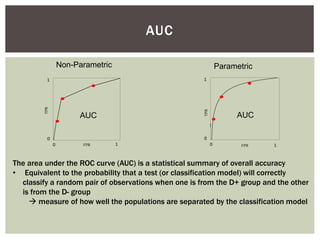
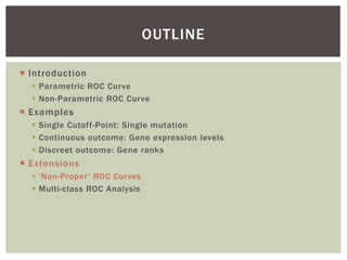
The document presents an introduction to ROC curve analysis applied in functional genomics, covering both parametric and non-parametric approaches. It includes concepts such as sensitivity, specificity, and Area Under the Curve (AUC), while providing examples of classification models concerning gene mutations and expression levels. Additionally, it discusses methods for evaluating model accuracy and extensions for multi-class ROC analysis.

1. Presented by:
Shana White
March 31, 2015
INTRODUCTION TO ROC
CURVE ANALYSIS WITH
APPLICATIONS IN
FUNCTIONAL GENOMICS

2.  Introduction
 Parametric ROC Curve
 Non-Parametric ROC Curve
 Examples
 Single Cutoff-Point: Single mutation
 Continuous outcome: Gene expression levels
 Discreet outcome: Gene ranks
 Extensions
 ‘Non-Proper’ ROC Curves
 Multi-class ROC Analysis
OUTLINE

3. ROC CURVES
 ROC = Receiver-operator characteristic (signal detection)
 Purpose: evaluation of classification model that predicts
binary group membership
 Model can be based on supervised or unsupervised methods, but ‘true’
group membership (as determined by ‘gold standard’) is known
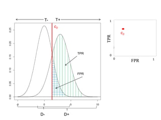
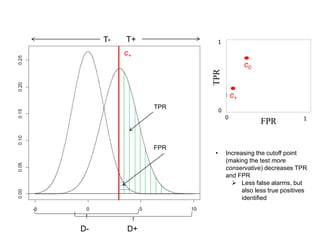
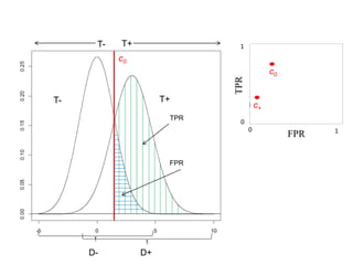
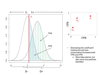
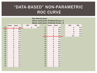
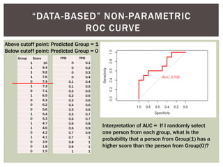
 Depict tradeoffs between sensitivity and specificity over a
range of cutoff values. In terms of disease:
 Sensitivity (True positive rate [TPR]): identification of those who
truly have the disease (D+) as having the disease (T+)
 Specificity (True negative rate [TNR]): identification of those that
do not actually have the disease (D-) as not having the disease (T-)
 The value [1-Specificity] (False positive rate [FPR]) is used in
graphs
 Ideal classification models have high TPR while maintaining low FPR
 TPR and FPR increase/decrease together

4. D- D+
c0
T- T+
TPR
FPR
0
FPR
0
1
1
TPR
c0

5. T+T-
D+D-
c+
TPR
FPR
• Increasing the cutoff point
(making the test more
conservative) decreases TPR
and FPR
 Less false alarms, but
also less true positives
identified
0
FPR
0
1
1
TPR
c+
c0

6. T+T-
D+D-
T+T-
c0
TPR
FPR
0
FPR
0
1
1
TPR
c+
c0

7. D+D-
0
FPR
0
1
1
TPR
c+
c0
• Decreasing the cutoff point
(making the test less
conservative) increases both
TPR and FPR
 More false alarms, but
also more true positives
identified
T+T-
c-
c-
TPR
FPR

8. 0
FPR0
1
1
TPR
0
FPR0
1
1
TPR
Non-Parametric Parametric
AUC AUC
The area under the ROC curve (AUC) is a statistical summary of overall accuracy
• Equivalent to the probability that a test (or classification model) will correctly
classify a random pair of observations when one is from the D+ group and the other
is from the D- group
 measure of how well the populations are separated by the classification model
AUC

9. 0
FPR0
1
1
TPR
TPRFPR
TPRFPR
TPRFPR
• AUC Values range: 0.5 – 1.0
• 0.5 - test is no better than
a random class
assignment
• 1.0 - perfect class
prediction

10. PARAMETRIC CALCULATION
(NORMAL DISTRIBUTION)
Let 𝑿0 and 𝑿1be test scores for 2 different populations of interest ( such
as no disease versus disease).
If 𝑋0 ~ 𝑁 𝜇0, 𝜎0 and 𝑋1 ~ 𝑁 𝜇1, 𝜎1 , then
AUC = 𝚽
𝑎
1+ 𝑏2
Where 𝑎 =
𝜇1−𝜇0
𝜎1
, 𝑏 =
𝜎0
𝜎1
, and 𝚽 is the cumulative
normal distribution function.
I think it helps to look at the equation a bit differently:
𝑎
1+ 𝑏2
=
𝜇1−𝜇0
𝜎1
1+
𝜎0
𝜎1
2
=
𝜇1−𝜇0
𝜎1
𝜎1
𝜎1
2
+
𝜎0
𝜎1
2
=
𝜇1−𝜇0
𝜎1
𝜎1
2 +𝜎0
2
𝜎1
=
𝜇1−𝜇0
𝜎1
2 +𝜎0
2
It is now readily apparent that AUC:
Increases as distance between means increases.
Decreases when standard deviations increase.
What happens if distance between means is 0?

11. “DATA-BASED” NON-PARAMETRIC
ROC CURVE
FPR TPR
0 0.1
0 0.2
0 0.3
0 0.4
0.1 0.4
Group Score
1 10
1 9.4
1 9.2
1 7.6
0 7.4
1 7.3
0 7.1
1 6.5
0 6.3
0 6.2
0 5.6
1 5.4
0 5.3
1 4.7
1 4.6
0 4.2
1 4.1
0 3.9
0 1.8
0 1.5
Sort data by score.
Above cutoff point: Predicted Group = 1
Below cutoff point: Predicted Group = 0
TP
FN
FN
FN
TN
FN
TN
FN
TN
TN
TN
FN
TN
FN
FN
TN
FN
TN
TN
TN
FPR TPR
0 0.1
Group Score
1 10
1 9.4
1 9.2
1 7.6
0 7.4
1 7.3
0 7.1
1 6.5
0 6.3
0 6.2
0 5.6
1 5.4
0 5.3
1 4.7
1 4.6
0 4.2
1 4.1
0 3.9
0 1.8
0 1.5
TP
TP
TP
TP
FP
FN
TN
FN
TN
TN
TN
FN
TN
FN
FN
TN
FN
TN
TN
TN

12. “DATA-BASED” NON-PARAMETRIC
ROC CURVE
FPR TPR
0 0.1
0 0.2
0 0.3
0 0.4
0.1 0.4
Group Score
1 10
1 9.4
1 9.2
1 7.6
0 7.4
1 7.3
0 7.1
1 6.5
0 6.3
0 6.2
0 5.6
1 5.4
0 5.3
1 4.7
1 4.6
0 4.2
1 4.1
0 3.9
0 1.8
0 1.5
0.1 0.5
0.2 0.5
0.2 0.6
0.3 0.6
0.4 0.6
0.5 0.6
0.5 0.7
0.6 0.7
0.6 0.8
0.6 0.9
0.7 0.9
0.7 1
0.8 1
0.9 1
1 1
Above cutoff point: Predicted Group = 1
Below cutoff point: Predicted Group = 0
Interpretation of AUC = If I randomly select
one person from each group, what is the
probability that a person from Group(1) has a
higher score than the person from Group(0)?

13. Group Score
0 1.5
0 6.2
0 5.3
0 4.2
0 3.9
0 7.1
0 5.6
0 7.4
0 1.8
0 6.3
1 9.2
1 10
1 4.1
1 6.5
1 5.4
1 9.4
1 4.6
1 7.3
1 4.7
1 7.6
USING RANKS TO BUILD AN ROC CURVE
Group Score Rank
1 10 1
1 9.4 2
1 9.2 3
1 7.6 4
0 7.4 5
1 7.3 6
0 7.1 7
1 6.5 8
0 6.3 9
0 6.2 10
0 5.6 11
1 5.4 12
0 5.3 13
1 4.7 14
1 4.6 15
0 4.2 16
1 4.1 17
0 3.9 18
0 1.8 19
0 1.5 20
Group Score
1 10
1 9.4
1 9.2
1 7.6
0 7.4
1 7.3
0 7.1
1 6.5
0 6.3
0 6.2
0 5.6
1 5.4
0 5.3
1 4.7
1 4.6
0 4.2
1 4.1
0 3.9
0 1.8
0 1.5
Group Rank
1 1
1 2
1 3
1 4
0 5
1 6
0 7
1 8
0 9
0 10
0 11
1 12
0 13
1 14
1 15
0 16
1 17
0 18
0 19
0 20

14. “RANK-BASED” NON-PARAMETRIC ROC
CURVE
Group Rank
1 1
1 2
1 3
1 4
0 5
1 6
0 7
1 8
0 9
0 10
0 11
1 12
0 13
1 14
1 15
0 16
1 17
0 18
0 19
0 20
1 - Specificity Sensitivity
0 0.1
0 0.2
0 0.3
0 0.4
0.1 0.4
0.1 0.5
0.2 0.5
0.2 0.6
0.3 0.6
0.4 0.6
0.5 0.6
0.5 0.7
0.6 0.7
0.6 0.8
0.6 0.9
0.7 0.9
0.7 1
0.8 1
0.9 1
1 1
Above cutoff point: Predicted Group = 1
Below cutoff point: Predicted Group = 0
Interpretation of AUC = If I randomly select
one person from each group, what is the
probability that a person from Group(1) is
ranked higher than the person from Group(0)?

15. RANK-BASED VS SCORE-BASED NON-
PARAMETRIC ROC CURVE
Curves are identical
Non-parametric (or “data–based” or “Empirical”) curves are inherently rank-based
“Rankiness”  nice statistical properties without the need to assume a
particular distribution

16. N0N-PARAMETRIC CALCULATION
Let 𝑿0 and 𝑿1be test scores OR ranks based on scores for 2 different
populations of interest (such as no disease versus disease).
If there is no distributional assumption for the values of 𝑿0 and 𝑿1, then
AUC =
1
𝑛0 𝑛1
𝑖=1
𝑛1
𝑗=1
𝑛2
𝐼(𝑋𝑖1, 𝑋𝑗0)
where 𝐼(𝑋𝑖1, 𝑋𝑗0) =
1 𝑖𝑓 𝑋𝑖1 > 𝑋𝑗0
1 2 𝑖𝑓 𝑋𝑖1 = 𝑋𝑗0
0 𝑖𝑓 𝑋𝑖1 < 𝑋𝑗0
AUC is equal to the Mann-Whitney U statistic; it compares the sums of ranks.
- Approximately normally distributed for large samples.
- Robust (not sensitive to outliers)

17.  Introduction
 Parametric ROC Curve
 Non-Parametric ROC Curve
 Examples
 Single Cutoff-Point: Single mutation
 Continuous outcome: Gene expression levels
 Discreet outcome: Gene ranks
 Extensions
 ‘Non-Proper’ ROC Curves
 Multi-class ROC Analysis
OUTLINE

18. EXAMPLE: SINGLE CUT-POINT,
SINGLE MUTATION
0 1
0 36 (TN) 4 (FN)
1 4 (FP) 16 (TP)
40 (P) 20(N)
Predicted Class
Based on BRCA1
status
(0 = WT, 1 = Mut)
True Class Based on Disease Outcome
( 0 = Negative for BC , 1 = Positive for BC)
Sensitivity (TPR)= TP/(TP + FN) =16/(16 +4) = 0.80
Specificity (TNR) = TN/(TN +FP) = 35/(35 + 4) = 0.90
Accuracy = (TP + TN)/(P + N) = (16+36)/(40 +20) = 0.8667
AUC = 0.85
FPR
TPR
AUC = 0.85

19. A CLOSER LOOK AT AUC
BC status = 0 BC status = 1
BRCA Mutation BRCA Mutation
0 0
0 0
0 0
0 0
0 1
0 1
0 1
0 1
0 1
0 1
0 1
0 1
0 1
0 1
0 1
0 1
0 1
0 1
0 1
0 1
0
0
0
0
0
0
0
0
0
0
0
0
0
0
0
0
1
1
1
1
TN = 36
FP = 4
TP = 16
FN = 4
Total number of pairwise comparisons :
(TN + FP)(FN + TP) = (40)(20) = 800
Number of times correct (𝑋𝑖1 > 𝑋𝑗0):
TN*TP = 576
Number of ties (𝑋𝑖1 = 𝑋𝑗0):
TP*FP + FN*TN = 64 + 144
AUC =
576+
1
2
(208)
800
=
680
800
= 0.85
For one cutoff point:
AUC =
2 𝑇𝑃∗𝑇𝑁 + 𝑇𝑃∗𝐹𝑃 +(𝑇𝑃∗𝐹𝑁)
2 𝑇𝑁+𝐹𝑃 (𝐹𝑁+𝑇𝑃)
=
𝑆𝑒𝑛𝑠.+𝑆𝑝𝑒𝑐.
2

20. A GEOMETRIC LOOK AT AUC
FPR
TPR
.5(0.1*0.8 )= 0.04
.5(1+0.8)*0.9 = 0.81
AUC via Trapezoidal Integration: 0.81 + 0.04 = 0.85
*ROC analysis is not typically performed for single cutoff scenarios but hopefully this
sheds light on the probabilistic/geometric nature of AUC

21.  Introduction
 Parametric ROC Curve
 Non-Parametric ROC Curve
 Examples
 Single Cutoff-Point: Single mutation
 Continuous outcome: Gene expression levels
 Discreet outcome: Gene ranks
 Extensions
 ‘Non-Proper’ ROC Curves
 Multi-class ROC Analysis
OUTLINE

22.  Hypothetical situation:
 I read about an cell-line experiment that found certain genes
upregulated in MCF-7 (breast cancer) cells. I want to see how the
results translate to human BC tumors.
 I choose two genes and go to the Genomics Portals website to obtain
gene expression data
Dataset: Breast invasive carcinoma from TCGA
Pubmed source: TCGA_BRCA_exp_HiSeqV2
Genes:
 IFI27 (interferon, alpha-inducible protein 27) – promotes cell death and is
associated with healing
 FN1 (fibronectin 1) - cell adhesion and migration processes
 How well do the corresponding gene expression levels discriminate
tumor samples from normal tissue samples?
EXAMPLE: CONTINUOUS OUTCOME -
GENE EXPRESSION LEVELS

23. EXAMPLE: CONTINUOUS OUTCOME -
GENE EXPRESSION LEVELS
Potential discriminatory gene #1 : IFI27
AUC = Probability that that if we randomly select one tumor and one normal sample
gene expression for IFI27(tumor) > gene expression for IFI27(normal)

24. EXAMPLE: CONTINUOUS OUTCOME -
GENE EXPRESSION LEVELS
Potential discriminatory gene #2 : FN1
AUC = Probability that that if we randomly select one tumor and one normal sample
gene expression for FN1(tumor) > gene expression for FN1(normal)

25. EXAMPLE: CONTINUOUS OUTCOME -
GENE EXPRESSION LEVELS
Is FN1 significantly better at discriminating amongst BC tumor samples than IFI27?
Note: pROC takes into account correlation between measurements when determining significance
P-value = 1.06 e-46 P-value = 4.69 e-42

26. A CLOSER LOOK: DATA DISTRIBUTIONS
Tumor   Normal
FN1
IFI27

27. EXAMPLE: CONTINUOUS OUTCOME -
GENE EXPRESSION LEVELS
I decide to go with FN1, now I want to know a little more.

28.  Introduction
 Parametric ROC Curve
 Non-Parametric ROC Curve
 Examples
 Single Cutoff-Point: Single mutation
 Continuous outcome: Gene expression levels
 Discreet outcome: Gene ranks
 Extensions
 ‘Non-Proper’ ROC Curves
 Multi-class ROC Analysis
OUTLINE

29. Hypothetical situation:
 I have been using DEseq for differential expression analysis. I
want to start using edgeR, but I hear it is less conservative
than DEseq.
 Since edgeR is less conservative, I am concerned that it will return
more false positives than DEseq.
 On the other hand, I am concerned that DEseq will return less true
positives than edgeR.
 I construct a simulation data set to represent two groups and
expression levels for 50 genes.
 I choose at random 20 genes to be up- or down-regulated (DE) between
groups when I simulate the data
 (for more detail see Soneson & Delorenzi 2013)
 I run DE on DEseq and edgeR and then rank the genes by p-value.
EXAMPLE: DISCREET OUTCOME -
RANKING OF DE GENES

30. EXAMPLE: DISCREET OUTCOME
DATA SET-UP
GeneID DEstatus rankedgeR rankDEseq
gene1 1 1 1
gene2 1 2 2
gene3 1 3 3
gene4 1 4 4
gene5 1 5 5
gene6 1 6 6
gene7 1 8 7
gene8 1 9 8
gene9 1 11 9
gene10 1 13 10
gene11 1 14 11
gene12 1 15 12
gene13 1 17 14
gene14 1 20 15
. . . .
. . . .
. . . .
gene37 0 37 35
gene38 0 38 36
gene39 0 39 37
gene40 0 40 39
gene41 0 41 40
gene42 0 42 41
gene43 0 43 42
gene44 0 44 43
gene45 0 45 44
gene46 0 46 46
gene47 0 47 47
gene48 0 48 48
gene49 0 49 49
gene50 0 50 50

31. ROC CURVES FOR GENE RANKS
AUC = Probability that that if we randomly select one DE and one non-DE gene:
gene rank(DE gene) > gene rank (non-DE gene)

32. DIFFERENCES IN PERFORMANCE
Is there another way to identify differences in performance?

33. COMPARISON OVER SPECIFIC FPR
p-value for difference in pAUC= 0.001041
If we are mainly focused on maintaining a low FPR, DEseq outperforms edgeR

34. COMPARISON OVER SPECIFIC TPR
p-value for difference in pAUC= 0.03188
If we want to identify as many genes as possible, edgeR outperforms DEseq at a
lower threshold

35.  Introduction
 Parametric ROC Curve
 Non-Parametric ROC Curve
 Examples
 Single Cutoff-Point: Single mutation
 Continuous outcome: Gene expression levels
 Discreet outcome: Gene ranks
 Extensions
 ‘Non-Proper’ ROC Curves
 Multi-class ROC Analysis
OUTLINE

36. SCENARIOS FOR ‘NOT-PROPER’ ROC
CURVES
Parodi et al. BMC Bioinformatics 2008
9:410 doi:10.1186/1471-2105-9-410

37. SIMPLIFIED SCENARIO: SAME MEAN,
DIFFERENT SD’S
𝐴𝑈𝐶 = 𝚽
𝜇1−𝜇0
𝜎1
2 +𝜎0
2

38.  Rationale: If there is no difference in mean measurement
between groups, we are ‘constrained’ to have AUC = 0.50
 Useful if difference in measurements between groups is not reflected
by an overall difference in means.
 Can account for bimodal distributions, ‘nested’ distributions
 May capture unique aspects of biological variability
 ABCR = area between the ROC curve and the rising diagonal
 TNRC = Test for Not-proper ROC Curves
ANALYSIS WITH NOT-PROPER ROCS

39.  Introduction
 Parametric ROC Curve
 Non-Parametric ROC Curve
 Examples
 Single Cutoff-Point: Single mutation
 Continuous outcome: Gene expression levels
 Discreet outcome: Gene ranks
 Extensions
 ‘Non-Proper’ ROC Curves
 Multi-class ROC Analysis
OUTLINE

40.  Oftentimes, category labels are made binary for ease of
interpretation and/or analysis
 Ex) [cancer, no cancer], [normal, abnormal], [positive, negative]
 Traditional ROC methods adhere to this ‘rule’
 If there is more than one class we are interested in, we have to ‘force
dichotomization’ by combining two [or more] classes
 Ex) Types of breast cancer (LA, LB, HER2, Basal) would all be classified as
cancer if compared to normal
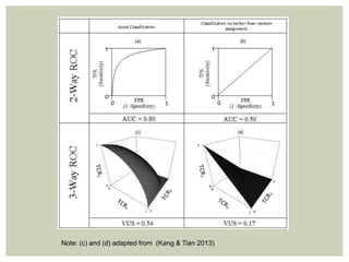
 Multi-class ROC methods are natural extensions of traditional
methods
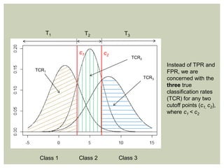
 Instead of area [under the curve], we are interested in volume under
the surface (VUS, 3-classes) or hypervolume under the manifold
(HUM, more than three classes)
 Baseline value for comparison:
1
𝑘!
where k = number of classes
MULTI-CLASS R0C

41. Class 1 Class 2 Class 3
c1 c2
T1 T2 T3
TCR1
Instead of TPR and
FPR, we are
concerned with the
three true
classification rates
(TCR) for any two
cutoff points (c1, c2),
where c1 < c2
TCR2
TCR3

42. VOLUME UNDER THE SURFACE
 Each possible pair of cutoff points yields a triplet of
true classification rates
 Triplet is coordinates for point in 3-D space
 Points are plotted and connected to form an ROC surface
 Volume under the ROC surface (VUS) is analogous to AUC
 VUS of
1
6
(≈ 0.167) indicative of random class assignment
Non-Parametric (Nakas & Yiannoutsos 2004)Parametric (Kang & Tian 2013)

43. Note: (c) and (d) adapted from (Kang & Tian 2013)

44. EXAMPLE: MICROSATELLITE INSTABILITY
IN COLON CANCER
 Microsatellite instability (MSI) has been associated with colon
cancer. Results from a panel of genetic markers are used to
determine MSI status on three levels:
1. MSS: microsatellite stable, no markers detected
2. MSI-L: MSI-Low; at least 1 but < 30% across panel
3. MSI-H: MSI-High; > 30% mutation rate across panel
 I read a paper (Molecular Cancer 2007, 6:54 ) that says they found a
gene that is upregulated in MSI-H vs. MSS-type tumors (they
dichotomized their data)
 I want to see if these findings also apply to tumor samples and extend to a
three-level classification system.
Gene: SECTM1
Data: Colon adenocarcinomas from TCGA
Pubmed source= TCGA_COAD_exp_HiSeqV2

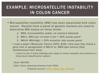
45. EXAMPLE: MICROSATELLITE INSTABILITY
IN COLON CANCER
[Edited] Raw Data Summary:
n mu sd
Level 1: MSS 98 8.21 1.17
Level 2: MSI-L 25 8.03 1.29
Level 3: MSI-H 25 10.05 1.49
VUS=0.3419, 95% CI=[0.2258, 0.457]
Best cut-points: lower(c1)=8.0439, upper(c2)=9.3773
The group correct classification probabilities are
MSS MSH-L MSH-H
0.4184 0.6429 0.8000
VUS = Probability that if we choose at random one MSS, MSI-L and MSI-H sample:
SECTM1MSS < SECTM1MSI-L < SECTM1MSI-H

46. EXAMPLE: MICROSATELLITE INSTABILITY
IN COLON CANCER
[Edited] Raw Data Summary:
n mu sd
Level 1: MSI-L 25 8.03 1.29
Level 2: MSS 98 8.21 1.17
Level 3: MSI-H 25 10.05 1.49
VUS(new)=0.4692, 95% CI=[0.3289, 0.6017]
VUS(old)=0.3419
Best cut-points: lower(c1)=7.4214, upper(c2)=9.3773
The group correct classification probabilities are
MSS MSH-L MSH-H
0.4184 0.4400 0.8000
VUS = Probability that if we choose at random one MSS, MSI-L and MSI-H sample:
SECTM1MSI-L < SECTM1MSS < SECTM1MSI-H

47. SOMETHING TO CONSIDER:
REMEMBER IFI27?
 The original AUC was not very
impressive, but levels are
moderately higher in tumors
 Brief literature review yields info
that IFI27 upregulation has been
implicated in epithelial cancer
cells.
 Can we gain further insight if we
stratify by cell type?
 We can’t do this with the TCGA
data, but Genomics Portal has a
different data set I can use
 Tumor and normal tissue samples
classified as either epithelial or
squamous
 PubMed source= GSE10797,

48.  Heterogeneity of BC
adds ‘noise’ to the ROC
analysis
 Keeping in mind small
sample size, a few
sources in this case
include:
 Higher levels of IFI27
measured in normal
stromal cells
 An ‘island’ of cancerous
epithelial cells with
marked IFI27
upregulation
SOMETHING TO CONSIDER:
REMEMBER IFI27?

49.  Flexible tool for evaluating classification models
 Provides statistical and graphical measures of overall accuracy
 Yields optimal cutoff values for prediction
 Some considerations for use in functional genomics:
 Heterogeneity of biological data
 We are using relatively simple methods but dealing with appreciably
complex phenomena
 Unequal sample sizes for groups
 Generally more cancer samples than normal samples
 More genes are non-DE vs DE (when considering ranking systems)
 This is only the tip of the iceberg!
 Bayesian methods, semi-parametric methods, misclassification costs,
training/validation issues, multivariable models…
SUMMARY OF ROC ANALYSIS

50. QUESTIONS?
http://stats.stackexchange.com/questions/423/what-is-your-favorite-data-analysis-cartoon?page=2&tab=votes#tab-top