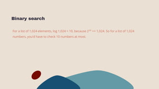
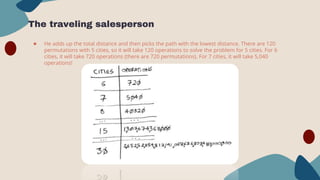
SlideShare a Scribd company logo
Algorithms
05
By Mohamed Essam
CONTENT OF THIS COURSE
Here’s what you’ll find in this Slidesgo template:
● Analyzing the algorithm.
● Linear search.
● Binary Search.
● Sorting.
Analyzing the algorithm
To create a good algorithm, we have to ensure that we have got the best performance
from the algorithm. In this section, we are going to discuss the ways we can analyze the
time complexity of basic functions.
Worst, average, and best cases
 Worst case analysis is a calculation of the upper bound on the running time of the
algorithm. In the Search() function, the upper bound can be an element that does not
appear in the arr, for instance, 60, so it has to iterate through all elements of arr and
still cannot find the element.
 Average case analysis is a calculation of all possible inputs on the running time of
algorithm, including an element that is not present in the arr array.
 Best case analysis is a calculation of the lower bound on the running time of the
algorithm. In the Search() function, the lower bound is the first element of the arr array,
which is 42. When we search for element 42, the function will only iterate through the
arr array once, so the arrSize doesn't matter.
Big Theta, Big-O, and Big Omega
After discussing asymptotic analysis and the three cases in algorithms, let's discuss
asymptotic notation to represent the time complexity of an algorithm. There are three
asymptotic notations that are mostly used in an algorithm; they are Big Theta, Big-O, and
Big Omega
Big Theta, Big-O, and Big Omega
The Big Theta notation (θ) is a notation that bounds a function from above and below, like
we saw previously in asymptotic analysis, which also omits a constant from a notation.
Big Theta, Big-O, and Big Omega
Big-O notation (O) is a notation that bounds a function from above only using the upper
bound of an algorithm. From the previous notation, f(n) = 4n + 1, we can say that the time
complexity of the f(n) is O(n). If we are going to use Big Theta notation, we can say that the
worst case time complexity of f(n) is θ(n) and the best case time complexity of f(n) is θ(1).
Big Theta, Big-O, and Big Omega
Big Omega notation is contrary to Big-O notation. It uses the lower bound to analyze time
complexity. In other words, it uses the best case in Big Theta notation. For the f(n)
notation, we can say that the time complexity is Ω(1).
O(N) — "worst case" definition
In the worst case, I need to do approximately N steps for an input of size N.
O(N) — "scaling" definition
For every new item that gets added to my input, I need to do a new step. We say "our runtime
scales linearly with the size of our input".
Ω(1) — "best case" definition
In the best case, I only need to do a constant number of steps to find my solution.
O(N2) — "worst case" definition
In the worst case, I need to do approximately N2 steps if
my input size is N.
Ω(N2) — "best case" definition
In the worst case, I need to do approximately N2 steps if
my input size is N.
O(N2) — "scaling" definition
In the worst case, I need to do approximately N2 steps if
my input size is N.
Ω(N) — "best case" definition
In the best case, I need to do approximately N steps if
my input size is N.
O(log2(n)) — "worst case" definition
In the worst case, I need to do log2(n) steps to find my
solution.
O(log2(n)) — "scaling" definition
I don't need to take another step in my algorithm until I
double my input.
Binary search
Suppose you’re searching for a word in a Dictionary. The word starts with K. You could
start at the beginning and keep flipping pages until you get to the Ks. But you’re more likely
to start at a page in the middle, because you know the Ks are going to be near the middle
of the Dictionary.
Binary search
Binary search
Now suppose you log on to Facebook. When you do, Facebook has to verify that you have an
account on the site. So, it needs to search for your username in its database. Suppose your
username is kareem. Facebook could start from the As and search for your name—but it
makes more sense for it to begin somewhere in the middle. This is a search problem. And all
these cases use the same algorithm to solve the problem: binary search.
Binary search
Binary search is an algorithm; its input is a sorted list of elements (I’ll explain later why it
needs to be sorted). If an element you’re looking for is in that list, binary search returns the
position where it’s located. Otherwise, binary search returns null.
Binary search
Binary search
Binary search
Suppose you’re looking for a word in the dictionary. The dictionary has 240,000 words. In the
worst case, how many steps do you think each search will take?
Simple search could take 240,000 steps if the word you’re looking for is the very last one in
the book. With each step of binary search, you cut the number of words in half until you’re
left with only one word.
Binary search
So binary search will take 18 steps—a big difference! In general, for any list of n, binary search
will take log2 n steps to run in the worst case, whereas simple search will take n steps.
Binary search
Binary search
For a list of 1,024 elements, log 1,024 = 10, because 210
== 1,024. So for a list of 1,024
numbers, you’d have to check 10 numbers at most.
Binary search
Binary search-Running time
 Generally you want to choose the most efficient algorithm— whether you’re trying to
optimize for time or space.
 Back to binary search. How much time do you save by using it? Well, the first approach
was to check each number, one by one. If this is a list of 100 numbers, it takes up to 100
guesses. If it’s a list of 4 billion numbers, it takes up to 4 billion guesses. So the maximum
number of guesses is the same as the size of the list. This is called linear time. Binary
search is different. If the list is 100 items long, it takes at most 7 guesses. If the list is 4
billion items, it takes at most 32 guesses. Powerful, eh? Binary search runs in logarithmic
time (or log time, as the natives call it). Here’s a table summarizing our findings today
Binary search
Binary search-Big O notation
 Big O notation is special notation that tells you how fast an algorithm is.
 Big O establishes a worst-case run time
Visualizing different Big O run times
 Here’s a practical example you can follow at home with a few pieces of paper and a pencil.
Suppose you have to draw a grid of 16 boxes.
 Algorithm 1 One way to do it is to draw 16 boxes, one at a time. Remember, Big O
notation counts the number of operations. In this example, drawing one box is one
operation. You have to draw 16 boxes. How many operations will it take, drawing
one box at a time?
Visualizing different Big O run times
 Algorithm 2 Try this algorithm instead. Fold the paper.
Visualizing different Big O run times
 You can “draw” twice as many boxes with every fold, so you can draw 16 boxes in 4 steps.
What’s the running time for this algorithm? Come up with running times for both
algorithms before moving on. Answers: Algorithm 1 takes O(n) time, and algorithm 2 takes
O(log n) time.
Some common Big O run times
 Here are five Big O run times that you’ll encounter a lot, sorted from fastest to slowest:
 O(log n), also known as log time. Example: Binary search.
 O(n), also known as linear time. Example: Simple search.
 O(n * log n). Example: A fast sorting algorithm, like quicksort .
 O(n2 ). Example: A slow sorting algorithm, like selection sort .
 O(n!). Example: A really slow algorithm, like the traveling salesperson.
Visualizing different Big O run times
 Algorithm speed isn’t measured in seconds, but in growth of
the number of operations.
 Instead, we talk about how quickly the run time of an
algorithm increases as the size of the input increases.
The traveling salesperson
You might have read that last section and thought, “There’s no way I’ll ever run
into an algorithm that takes O(n!) time.” Well, let me try to prove you wrong!
Here’s an example of an algorithm with a really bad running time. This is a
famous problem in computer science, because its growth is appalling and some
very smart people think it can’t be improved. It’s called the traveling salesperson
problem
The traveling salesperson
● You have a salesperson.
● The salesperson has to go to five cities.
● This salesperson, whom I’ll call Opus, wants to hit all five cities while traveling the minimum
distance. Here’s one way to do that: look at every possible order in which he could travel to the
cities.
The traveling salesperson
● He adds up the total distance and then picks the path with the lowest distance. There are 120
permutations with 5 cities, so it will take 120 operations to solve the problem for 5 cities. For 6
cities, it will take 720 operations (there are 720 permutations). For 7 cities, it will take 5,040
operations!
The traveling salesperson
In general, for n items, it will take n! (n factorial) operations to compute the result. So this is O(n!) time,
or factorial time. It takes a lot of operations for everything except the smallest numbers. Once you’re
dealing with 100+ cities, it’s impossible to calculate the answer in time—the Sun will collapse first. This is
a terrible algorithm! Opus should use a different one, right? But he can’t. This is one of the unsolved
problems in computer science. There’s no fast known algorithm for it, and smart people think it’s
impossible to have a smart algorithm for this problem. The best we can do is come up with an
approximate solution; see chapter 10 for more.
Selection Sort-How Memory Works
 Imagine you go to a show and need to check your things. A chest of drawers is available.
 Each drawer can hold one element. You want to store two things, so you ask for two drawers.
Selection Sort-How Memory Works
 Imagine you go to a show and need to check your things. A chest of drawers is available.
 Each drawer can hold one element. You want to store two things, so you ask for two drawers.
Selection Sort-How Memory Works
 You store your two things here.
Selection Sort-How Memory Works
 And you’re ready for the show! This is basically how your computer’s memory works. Your
computer looks like a giant set of drawers, and each drawer has an address.
 fe0ffeeb is the address of a slot in memory. / Each time you want to store an item in memory, you
ask the computer for some space, and it gives you an address where you can store your item. If you
want to store multiple items, there are two basic ways to do so: arrays and lists. I’ll talk about arrays
and lists next, as well as the pros and cons of each. There isn’t one right way to store items for
every use case, so it’s important to know the differences.
Arrays and linked lists
 Sometimes you need to store a list of elements in memory. Suppose you’re writing an app to
manage your todos. You’ll want to store the todos as a list in memory. Should you use an array, or a
linked list? Let’s store the todos in an array first, because it’s easier to grasp. Using an array means
all your tasks are stored contiguously (right next to each other) in memory.
Arrays and linked lists
 Now suppose you want to add a fourth task. But the next drawer is taken up by someone else’s
stuff!
 It’s like going to a movie with your friends and finding a place to sit— but another friend joins you,
and there’s no place for them. You have to move to a new spot where you all fit. In this case, you
need to ask your computer for a different chunk of memory that can fit four tasks. Then you need
to move all your tasks there.
Arrays and linked lists
 If another friend comes by, you’re out of room again—and you all have to move a second time!
What a pain. Similarly, adding new items to an array can be a big pain. If you’re out of space and
need to move to a new spot in memory every time, adding a new item will be really slow. One easy
fix is to “hold seats”: even if you have only 3 items in your task list, you can ask the computer for 10
slots, just in case. Then you can add 10 items to your task list without having to move.
Arrays and linked lists
 This is a good workaround, but you should be aware of a couple of downsides:
 You may not need the extra slots that you asked for, and then that memory will
be wasted. You aren’t using it, but no one else can use it either.
 You may add more than 10 items to your task list and have to move anyway. So
it’s a good workaround, but it’s not a perfect solution. Linked lists solve this
problem of adding items.
Linked lists
 With linked lists, your items can be anywhere in memory.
 Each item stores the address of the next item in the list. A bunch of random memory addresses are
linked together.
Which are used more: arrays or lists?
 Obviously, it depends on the use case. But arrays see a lot of use because they allow random
access. There are two different types of access: random access and sequential access. Sequential
access means reading the elements one by one, starting at the first element. Linked lists can only
do sequential access. If you want to read the 10th element of a linked list, you have to read the first
9 elements and follow the links to the 10th element. Random access means you can jump directly
to the 10th element. You’ll frequently hear me say that arrays are faster at reads. This is because
they provide random access. A lot of use cases require random access, so arrays are used a lot.
Arrays and lists are used to implement other data structures, too
EXERCISES
 Would you use an array or a linked list to implement this queue? (Hint: Linked lists are good for
inserts/deletes, and arrays are good for random access. Which one are you going to be doing here?)
 Let’s run a thought experiment. Suppose Facebook keeps a list of usernames. When someone tries
to log in to Facebook, a search is done for their username. If their name is in the list of usernames,
they can log in. People log in to Facebook pretty often, so there are a lot of searches through this
list of usernames. Suppose Facebook uses binary search to search the list. Binary search needs
random access—you need to be able to get to the middle of the list of usernames instantly.
Knowing this, would you implement the list as an array or a linked list?
Bubble Sort
The Bubble Sort compares each successive pair of elements
in an unordered list and inverts the elements if they are not in
order.
Bubble Sort
Selection Sort
Selection sort is a sorting algorithm, specifically an in-place comparison sort. It has O(n2)
time complexity, making it inefficient on large lists, and generally performs worse than
the similar insertion sort. Selection sort is noted for its simplicity, and it has performance
advantages over more complicated algorithms in certain situations, particularly where
auxiliary memory is limited. The algorithm divides the input list into two parts: the sublist
of items already sorted, which is built up from left to right at the front (left) of the list, and
the sublist of items remaining to be sorted that occupy the rest of the list. Initially, the
sorted sublist is empty and the unsorted sublist is the entire input list. The algorithm
proceeds by finding the smallest (or largest, depending on sorting order) element in the
unsorted sublist, exchanging (swapping) it with the leftmost unsorted element (putting it
in sorted order), and moving the sublist boundaries one element to the right.
Selection Sort
 Suppose you have a bunch of music on your computer. For each artist, you have a play count.
 You want to sort this list from most to least played, so that you can rank your favorite artists. How
can you do it?
Selection Sort
 One way is to go through the list and find the most-played artist. Add that artist to a new list.
Selection Sort
 Keep doing this, and you’ll end up with a sorted list.
Selection Sort
 Let’s put on our computer science hats and see how long this will take to run. Remember that O(n)
time means you touch every element in a list once. For example, running simple search over the list
of artists means looking at each artist once
Selection Sort
 To find the artist with the highest play count, you have to check each item in the list. This takes O(n)
time, as you just saw. So you have an operation that takes O(n) time, and you have to do that n
times:
 This takes O(n × n) time or O(n2 ) time.
Selection Sort
Merge Sort
Merge Sort is a divide-and-conquer algorithm. It divides the input list of length n in
half successively until there are n lists of size 1. Then, pairs of lists are merged
together with the smaller first element among the pair of lists being added in each
step. Through successive merging and through comparison of first elements, the
sorted list is built.
Merge Sort
Greedy Algorithm
When using a device like this, odds are you want to minimize the
number of coins you’re dispensing for each customer, lest you
have to press levers more times than are necessary. Fortunately,
computer science has given cashiers everywhere ways to
minimize numbers of coins due: greedy algorithms.
Greedy Algorithm
According to the National Institute of Standards and Technology
(NIST), a greedy algorithm is one "that always takes the best
immediate, or local, solution while finding an answer. Greedy
algorithms find the overall, or globally, optimal solution for some
optimization problems, but may find less-than-optimal solutions for
some instances of other problems.
Greedy Algorithm
What’s all that mean? Well, suppose that a cashier owes a customer
some change and on that cashier’s belt are levers that dispense quarters,
dimes, nickels, and pennies. Solving this "problem" requires one or more
presses of one or more levers. Think of a "greedy" cashier as one who
wants to take, with each press, the biggest bite out of this problem as
possible. For instance, if some customer is owed 41¢, the biggest first
(i.e., best immediate, or local) bite that can be taken is 25¢. (That bite is
"best" inasmuch as it gets us closer to 0¢ faster than any other coin
would.)
Greedy Algorithm
Note that a bite of this size would whittle what was a 41¢ problem down to
a 16¢ problem, since 41 - 25 = 16. That is, the remainder is a similar but
smaller problem. Needless to say, another 25¢ bite would be too big
(assuming the cashier prefers not to lose money), and so our greedy
cashier would move on to a bite of size 10¢, leaving him or her with a 6¢
problem. At that point, greed calls for one 5¢ bite followed by one 1¢ bite,
at which point the problem is solved. The customer receives one quarter,
one dime, one nickel, and one penny: four coins in total.
Dynamic Programming
 The term "dynamic programming" was invented by Richard Bellman to
"sound cool" to management, ensuring that there would continue to be
funding for his research.
 In fact, dynamic programming is simply the concept of saving
computed results for reuse later, much like a lookup table.
 Just like how hash tables and tries are types of data structures,
dynamic programming is a type of algorithm that solves a problem by
saving the results each time, and looking up the answer if it’s needed
in the future, saving that extra computation.
Dynamic Programming
Breadth-first search
 Breadth-first search allows you to find the shortest distance between two
things. But shortest distance can mean a lot of things! You can use breadth-
first search to •
 Write a checkers AI that calculates the fewest moves to Univeristy
 Find the doctor closest to you in your network
Introduction to graphs
 Suppose you’re in San Francisco, and you want to go from Twin Peaks to the
Golden Gate Bridge. You want to get there by bus, with the minimum number
of transfers. Here are your options.
Introduction to graphs
 Aha! Now the Golden Gate Bridge shows up. So it takes three steps to get
from Twin Peaks to the bridge using this route.
Introduction to graphs
 There are other routes that will get you to the bridge too, but they’re longer
(four steps). The algorithm found that the shortest route to the bridge is
three steps long. This type of problem is called a shortest-path problem.
You’re always trying to find the shortest something. It could be the shortest
route to your friend’s house. It could be the smallest number of moves to
checkmate in a game of chess. The algorithm to solve a shortest-path
problem is called breadth-first search.
To figure out how to get from Twin Peaks to the Golden
Gate Bridge, there are two steps
1. Model the problem as a graph.(
○ What is a graph?
■ A graph models a set of connections.)
2. 2. Solve the problem using breadth-first search.
Breadth-first search
 We looked at a search algorithm in chapter 1: binary search. Breadthfirst
search is a different kind of search algorithm: one that runs on graphs. It can
help answer two types of questions: •
 Question type 1: Is there a path from node A to node B?
 Question type 2: What is the shortest path from node A to node B?
Knapsack Problem
Knapsack Problem
Recursion
● Suppose you’re digging through your grandma’s attic and come across a mysterious locked
suitcase.
● Grandma tells you that the key for the suitcase is probably in this other box.
● This box contains more boxes, with more boxes inside those boxes. The key is in a box somewhere.
What’s your algorithm to search for the key? Think of an algorithm before you read on.
Recursion
1. Make a pile of boxes to look through.
2. Grab a box, and look through it.
3. If you find a box, add it to the pile to look through later.
4. If you find a key, you’re done! 5.
5. Repeat.
Recursion
 Recursion is where a function calls itself. Here’s the second way in
pseudocode:
 Recursion is used when it makes the solution clearer. There’s no performance
benefit to using recursion; in fact, loops are sometimes better for
performance. I like this quote by Leigh Caldwell on Stack Overflow: “Loops may
achieve a performance gain for your program. Recursion may achieve a
performance gain for your programmer. Choose which is more important in
your situation!”1
Recursion
 You can write it recursively, like so:
Recursion
 Write out this code and run it. You’ll notice a problem: this function will run
forever!
Recursion
 When you write a recursive function, you have to tell it when to stop recursing.
That’s why every recursive function has two parts: the base case, and the
recursive case. The recursive case is when the function calls itself. The base
case is when the function doesn’t call itself again … so it doesn’t go into an
infinite loop.

More Related Content

What's hot

5.2 divide and conquer
5.2 divide and conquer5.2 divide and conquer
5.2 divide and conquer
Krish_ver2
 
Hashing Technique In Data Structures
Hashing Technique In Data StructuresHashing Technique In Data Structures
Hashing Technique In Data Structures
SHAKOOR AB
 
Vertex cover Problem
Vertex cover ProblemVertex cover Problem
Vertex cover Problem
Gajanand Sharma
 
Backtracking & branch and bound
Backtracking & branch and boundBacktracking & branch and bound
Backtracking & branch and bound
Vipul Chauhan
 
Intro automata theory
Intro automata theory Intro automata theory
Intro automata theory
Rajendran
 
Asymptotic notations
Asymptotic notationsAsymptotic notations
Asymptotic notationsNikhil Sharma
 
Graph data structure
Graph data structureGraph data structure
Graph data structureTech_MX
 
Graph in data structure
Graph in data structureGraph in data structure
Graph in data structure
Abrish06
 
Design and Analysis of Algorithms.pptx
Design and Analysis of Algorithms.pptxDesign and Analysis of Algorithms.pptx
Design and Analysis of Algorithms.pptx
Syed Zaid Irshad
 
Python Data Structures and Algorithms.pptx
Python Data Structures and Algorithms.pptxPython Data Structures and Algorithms.pptx
Python Data Structures and Algorithms.pptx
ShreyasLawand
 
Greedy Algorihm
Greedy AlgorihmGreedy Algorihm
Greedy Algorihm
Muhammad Amjad Rana
 
Sum of subset problem.pptx
Sum of subset problem.pptxSum of subset problem.pptx
Sum of subset problem.pptx
V.V.Vanniaperumal College for Women
 
N queen problem
N queen problemN queen problem
N queen problem
Ridhima Chowdhury
 
Unit 1 chapter 1 Design and Analysis of Algorithms
Unit 1   chapter 1 Design and Analysis of AlgorithmsUnit 1   chapter 1 Design and Analysis of Algorithms
Unit 1 chapter 1 Design and Analysis of Algorithms
P. Subathra Kishore, KAMARAJ College of Engineering and Technology, Madurai
 
Array linear data_structure_2 (1)
Array linear data_structure_2 (1)Array linear data_structure_2 (1)
Array linear data_structure_2 (1)eShikshak
 
Algorithms Lecture 1: Introduction to Algorithms
Algorithms Lecture 1: Introduction to AlgorithmsAlgorithms Lecture 1: Introduction to Algorithms
Algorithms Lecture 1: Introduction to Algorithms
Mohamed Loey
 
Polynomial reppresentation using Linkedlist-Application of LL.pptx
Polynomial reppresentation using Linkedlist-Application of LL.pptxPolynomial reppresentation using Linkedlist-Application of LL.pptx
Polynomial reppresentation using Linkedlist-Application of LL.pptx
Albin562191
 
Queue ppt
Queue pptQueue ppt
Queue ppt
SouravKumar328
 
Compiler Design LR parsing SLR ,LALR CLR
Compiler Design LR parsing SLR ,LALR CLRCompiler Design LR parsing SLR ,LALR CLR
Compiler Design LR parsing SLR ,LALR CLR
Riazul Islam
 
Data Structure and Algorithms Hashing
Data Structure and Algorithms HashingData Structure and Algorithms Hashing
Data Structure and Algorithms Hashing
ManishPrajapati78
 

What's hot (20)

5.2 divide and conquer
5.2 divide and conquer5.2 divide and conquer
5.2 divide and conquer
 
Hashing Technique In Data Structures
Hashing Technique In Data StructuresHashing Technique In Data Structures
Hashing Technique In Data Structures
 
Vertex cover Problem
Vertex cover ProblemVertex cover Problem
Vertex cover Problem
 
Backtracking & branch and bound
Backtracking & branch and boundBacktracking & branch and bound
Backtracking & branch and bound
 
Intro automata theory
Intro automata theory Intro automata theory
Intro automata theory
 
Asymptotic notations
Asymptotic notationsAsymptotic notations
Asymptotic notations
 
Graph data structure
Graph data structureGraph data structure
Graph data structure
 
Graph in data structure
Graph in data structureGraph in data structure
Graph in data structure
 
Design and Analysis of Algorithms.pptx
Design and Analysis of Algorithms.pptxDesign and Analysis of Algorithms.pptx
Design and Analysis of Algorithms.pptx
 
Python Data Structures and Algorithms.pptx
Python Data Structures and Algorithms.pptxPython Data Structures and Algorithms.pptx
Python Data Structures and Algorithms.pptx
 
Greedy Algorihm
Greedy AlgorihmGreedy Algorihm
Greedy Algorihm
 
Sum of subset problem.pptx
Sum of subset problem.pptxSum of subset problem.pptx
Sum of subset problem.pptx
 
N queen problem
N queen problemN queen problem
N queen problem
 
Unit 1 chapter 1 Design and Analysis of Algorithms
Unit 1   chapter 1 Design and Analysis of AlgorithmsUnit 1   chapter 1 Design and Analysis of Algorithms
Unit 1 chapter 1 Design and Analysis of Algorithms
 
Array linear data_structure_2 (1)
Array linear data_structure_2 (1)Array linear data_structure_2 (1)
Array linear data_structure_2 (1)
 
Algorithms Lecture 1: Introduction to Algorithms
Algorithms Lecture 1: Introduction to AlgorithmsAlgorithms Lecture 1: Introduction to Algorithms
Algorithms Lecture 1: Introduction to Algorithms
 
Polynomial reppresentation using Linkedlist-Application of LL.pptx
Polynomial reppresentation using Linkedlist-Application of LL.pptxPolynomial reppresentation using Linkedlist-Application of LL.pptx
Polynomial reppresentation using Linkedlist-Application of LL.pptx
 
Queue ppt
Queue pptQueue ppt
Queue ppt
 
Compiler Design LR parsing SLR ,LALR CLR
Compiler Design LR parsing SLR ,LALR CLRCompiler Design LR parsing SLR ,LALR CLR
Compiler Design LR parsing SLR ,LALR CLR
 
Data Structure and Algorithms Hashing
Data Structure and Algorithms HashingData Structure and Algorithms Hashing
Data Structure and Algorithms Hashing
 

Similar to Introduction to Algorithms

Algorithms
Algorithms Algorithms
Algorithms
Mohamed Essam
 
Interview questions slide deck
Interview questions slide deckInterview questions slide deck
Interview questions slide deck
MikeBegley
 
Analysis of algorithms
Analysis of algorithmsAnalysis of algorithms
Analysis of algorithms
Mallikarjun Biradar
 
Element distinctness lower bounds
Element distinctness lower boundsElement distinctness lower bounds
Element distinctness lower bounds
Rajendran
 
daa unit 1.pptx
daa unit 1.pptxdaa unit 1.pptx
daa unit 1.pptx
LakshayYadav46
 
L1803016468
L1803016468L1803016468
L1803016468
IOSR Journals
 
9 big o-notation
9 big o-notation9 big o-notation
9 big o-notationirdginfo
 
Basics in algorithms and data structure
Basics in algorithms and data structure Basics in algorithms and data structure
Basics in algorithms and data structure Eman magdy
 
Complexity
ComplexityComplexity
Complexity
Malainine Zaid
 
Data Structures and Algorithms - Lec 02.pdf
Data Structures and Algorithms - Lec 02.pdfData Structures and Algorithms - Lec 02.pdf
Data Structures and Algorithms - Lec 02.pdf
RameshaFernando2
 
constructing_generic_algorithms__ben_deane__cppcon_2020.pdf
constructing_generic_algorithms__ben_deane__cppcon_2020.pdfconstructing_generic_algorithms__ben_deane__cppcon_2020.pdf
constructing_generic_algorithms__ben_deane__cppcon_2020.pdf
SayanSamanta39
 
DA lecture 3.pptx
DA lecture 3.pptxDA lecture 3.pptx
DA lecture 3.pptx
SayanSen36
 
Searching.pptx
Searching.pptxSearching.pptx
Searching.pptx
VenkataRaoS1
 
Sienna 13 limitations
Sienna 13 limitationsSienna 13 limitations
Sienna 13 limitationschidabdu
 
Csallner algorithms1
Csallner algorithms1Csallner algorithms1
Csallner algorithms1
seshagiri rao
 
Systems in the small - Introduction to Algorithms
Systems in the small - Introduction to AlgorithmsSystems in the small - Introduction to Algorithms
Systems in the small - Introduction to Algorithms
David Millard
 
Ds
DsDs
Chapter 4 algorithmic efficiency handouts (with notes)
Chapter 4   algorithmic efficiency handouts (with notes)Chapter 4   algorithmic efficiency handouts (with notes)
Chapter 4 algorithmic efficiency handouts (with notes)
mailund
 

Similar to Introduction to Algorithms (20)

Algorithms
Algorithms Algorithms
Algorithms
 
Interview questions slide deck
Interview questions slide deckInterview questions slide deck
Interview questions slide deck
 
Analysis of algorithms
Analysis of algorithmsAnalysis of algorithms
Analysis of algorithms
 
Element distinctness lower bounds
Element distinctness lower boundsElement distinctness lower bounds
Element distinctness lower bounds
 
daa unit 1.pptx
daa unit 1.pptxdaa unit 1.pptx
daa unit 1.pptx
 
L1803016468
L1803016468L1803016468
L1803016468
 
9 big o-notation
9 big o-notation9 big o-notation
9 big o-notation
 
Basics in algorithms and data structure
Basics in algorithms and data structure Basics in algorithms and data structure
Basics in algorithms and data structure
 
Complexity
ComplexityComplexity
Complexity
 
Data Structures and Algorithms - Lec 02.pdf
Data Structures and Algorithms - Lec 02.pdfData Structures and Algorithms - Lec 02.pdf
Data Structures and Algorithms - Lec 02.pdf
 
constructing_generic_algorithms__ben_deane__cppcon_2020.pdf
constructing_generic_algorithms__ben_deane__cppcon_2020.pdfconstructing_generic_algorithms__ben_deane__cppcon_2020.pdf
constructing_generic_algorithms__ben_deane__cppcon_2020.pdf
 
DA lecture 3.pptx
DA lecture 3.pptxDA lecture 3.pptx
DA lecture 3.pptx
 
Searching.pptx
Searching.pptxSearching.pptx
Searching.pptx
 
Sienna 13 limitations
Sienna 13 limitationsSienna 13 limitations
Sienna 13 limitations
 
Csallner algorithms1
Csallner algorithms1Csallner algorithms1
Csallner algorithms1
 
Big o
Big oBig o
Big o
 
Systems in the small - Introduction to Algorithms
Systems in the small - Introduction to AlgorithmsSystems in the small - Introduction to Algorithms
Systems in the small - Introduction to Algorithms
 
Ds
DsDs
Ds
 
Chapter 4 algorithmic efficiency handouts (with notes)
Chapter 4   algorithmic efficiency handouts (with notes)Chapter 4   algorithmic efficiency handouts (with notes)
Chapter 4 algorithmic efficiency handouts (with notes)
 
Time Complexity Analysis in Data Structure.docx
Time Complexity Analysis in Data Structure.docxTime Complexity Analysis in Data Structure.docx
Time Complexity Analysis in Data Structure.docx
 

More from Mohamed Essam

Data Science Crash course
Data Science Crash courseData Science Crash course
Data Science Crash course
Mohamed Essam
 
2.Feature Extraction
2.Feature Extraction2.Feature Extraction
2.Feature Extraction
Mohamed Essam
 
Data Science
Data ScienceData Science
Data Science
Mohamed Essam
 
Introduction to Robotics.pptx
Introduction to Robotics.pptxIntroduction to Robotics.pptx
Introduction to Robotics.pptx
Mohamed Essam
 
Introduction_to_Gui_with_tkinter.pptx
Introduction_to_Gui_with_tkinter.pptxIntroduction_to_Gui_with_tkinter.pptx
Introduction_to_Gui_with_tkinter.pptx
Mohamed Essam
 
Getting_Started_with_DL_in_Keras.pptx
Getting_Started_with_DL_in_Keras.pptxGetting_Started_with_DL_in_Keras.pptx
Getting_Started_with_DL_in_Keras.pptx
Mohamed Essam
 
Linear_algebra.pptx
Linear_algebra.pptxLinear_algebra.pptx
Linear_algebra.pptx
Mohamed Essam
 
Let_s_Dive_to_Deep_Learning.pptx
Let_s_Dive_to_Deep_Learning.pptxLet_s_Dive_to_Deep_Learning.pptx
Let_s_Dive_to_Deep_Learning.pptx
Mohamed Essam
 
OOP-Advanced_Programming.pptx
OOP-Advanced_Programming.pptxOOP-Advanced_Programming.pptx
OOP-Advanced_Programming.pptx
Mohamed Essam
 
1.Basic_Syntax
1.Basic_Syntax1.Basic_Syntax
1.Basic_Syntax
Mohamed Essam
 
Regularization_BY_MOHAMED_ESSAM.pptx
Regularization_BY_MOHAMED_ESSAM.pptxRegularization_BY_MOHAMED_ESSAM.pptx
Regularization_BY_MOHAMED_ESSAM.pptx
Mohamed Essam
 
1.What_if_Adham_Nour_tried_to_make_a_Machine_Learning_Model_at_Home.pptx
1.What_if_Adham_Nour_tried_to_make_a_Machine_Learning_Model_at_Home.pptx1.What_if_Adham_Nour_tried_to_make_a_Machine_Learning_Model_at_Home.pptx
1.What_if_Adham_Nour_tried_to_make_a_Machine_Learning_Model_at_Home.pptx
Mohamed Essam
 
Clean_Code
Clean_CodeClean_Code
Clean_Code
Mohamed Essam
 
Linear_Regression
Linear_RegressionLinear_Regression
Linear_Regression
Mohamed Essam
 
2.Data_Strucures_and_modules.pptx
2.Data_Strucures_and_modules.pptx2.Data_Strucures_and_modules.pptx
2.Data_Strucures_and_modules.pptx
Mohamed Essam
 
Naieve_Bayee.pptx
Naieve_Bayee.pptxNaieve_Bayee.pptx
Naieve_Bayee.pptx
Mohamed Essam
 
Activation_function.pptx
Activation_function.pptxActivation_function.pptx
Activation_function.pptx
Mohamed Essam
 
Deep_Learning_Frameworks
Deep_Learning_FrameworksDeep_Learning_Frameworks
Deep_Learning_Frameworks
Mohamed Essam
 
Neural_Network
Neural_NetworkNeural_Network
Neural_Network
Mohamed Essam
 

More from Mohamed Essam (20)

Data Science Crash course
Data Science Crash courseData Science Crash course
Data Science Crash course
 
2.Feature Extraction
2.Feature Extraction2.Feature Extraction
2.Feature Extraction
 
Data Science
Data ScienceData Science
Data Science
 
Introduction to Robotics.pptx
Introduction to Robotics.pptxIntroduction to Robotics.pptx
Introduction to Robotics.pptx
 
Introduction_to_Gui_with_tkinter.pptx
Introduction_to_Gui_with_tkinter.pptxIntroduction_to_Gui_with_tkinter.pptx
Introduction_to_Gui_with_tkinter.pptx
 
Getting_Started_with_DL_in_Keras.pptx
Getting_Started_with_DL_in_Keras.pptxGetting_Started_with_DL_in_Keras.pptx
Getting_Started_with_DL_in_Keras.pptx
 
Linear_algebra.pptx
Linear_algebra.pptxLinear_algebra.pptx
Linear_algebra.pptx
 
Let_s_Dive_to_Deep_Learning.pptx
Let_s_Dive_to_Deep_Learning.pptxLet_s_Dive_to_Deep_Learning.pptx
Let_s_Dive_to_Deep_Learning.pptx
 
OOP-Advanced_Programming.pptx
OOP-Advanced_Programming.pptxOOP-Advanced_Programming.pptx
OOP-Advanced_Programming.pptx
 
1.Basic_Syntax
1.Basic_Syntax1.Basic_Syntax
1.Basic_Syntax
 
KNN.pptx
KNN.pptxKNN.pptx
KNN.pptx
 
Regularization_BY_MOHAMED_ESSAM.pptx
Regularization_BY_MOHAMED_ESSAM.pptxRegularization_BY_MOHAMED_ESSAM.pptx
Regularization_BY_MOHAMED_ESSAM.pptx
 
1.What_if_Adham_Nour_tried_to_make_a_Machine_Learning_Model_at_Home.pptx
1.What_if_Adham_Nour_tried_to_make_a_Machine_Learning_Model_at_Home.pptx1.What_if_Adham_Nour_tried_to_make_a_Machine_Learning_Model_at_Home.pptx
1.What_if_Adham_Nour_tried_to_make_a_Machine_Learning_Model_at_Home.pptx
 
Clean_Code
Clean_CodeClean_Code
Clean_Code
 
Linear_Regression
Linear_RegressionLinear_Regression
Linear_Regression
 
2.Data_Strucures_and_modules.pptx
2.Data_Strucures_and_modules.pptx2.Data_Strucures_and_modules.pptx
2.Data_Strucures_and_modules.pptx
 
Naieve_Bayee.pptx
Naieve_Bayee.pptxNaieve_Bayee.pptx
Naieve_Bayee.pptx
 
Activation_function.pptx
Activation_function.pptxActivation_function.pptx
Activation_function.pptx
 
Deep_Learning_Frameworks
Deep_Learning_FrameworksDeep_Learning_Frameworks
Deep_Learning_Frameworks
 
Neural_Network
Neural_NetworkNeural_Network
Neural_Network
 

Recently uploaded

Essentials of Automations: Optimizing FME Workflows with Parameters
Essentials of Automations: Optimizing FME Workflows with ParametersEssentials of Automations: Optimizing FME Workflows with Parameters
Essentials of Automations: Optimizing FME Workflows with Parameters
Safe Software
 
Builder.ai Founder Sachin Dev Duggal's Strategic Approach to Create an Innova...
Builder.ai Founder Sachin Dev Duggal's Strategic Approach to Create an Innova...Builder.ai Founder Sachin Dev Duggal's Strategic Approach to Create an Innova...
Builder.ai Founder Sachin Dev Duggal's Strategic Approach to Create an Innova...
Ramesh Iyer
 
Smart TV Buyer Insights Survey 2024 by 91mobiles.pdf
Smart TV Buyer Insights Survey 2024 by 91mobiles.pdfSmart TV Buyer Insights Survey 2024 by 91mobiles.pdf
Smart TV Buyer Insights Survey 2024 by 91mobiles.pdf
91mobiles
 
How world-class product teams are winning in the AI era by CEO and Founder, P...
How world-class product teams are winning in the AI era by CEO and Founder, P...How world-class product teams are winning in the AI era by CEO and Founder, P...
How world-class product teams are winning in the AI era by CEO and Founder, P...
Product School
 
Epistemic Interaction - tuning interfaces to provide information for AI support
Epistemic Interaction - tuning interfaces to provide information for AI supportEpistemic Interaction - tuning interfaces to provide information for AI support
Epistemic Interaction - tuning interfaces to provide information for AI support
Alan Dix
 
Key Trends Shaping the Future of Infrastructure.pdf
Key Trends Shaping the Future of Infrastructure.pdfKey Trends Shaping the Future of Infrastructure.pdf
Key Trends Shaping the Future of Infrastructure.pdf
Cheryl Hung
 
JMeter webinar - integration with InfluxDB and Grafana
JMeter webinar - integration with InfluxDB and GrafanaJMeter webinar - integration with InfluxDB and Grafana
JMeter webinar - integration with InfluxDB and Grafana
RTTS
 
GraphRAG is All You need? LLM & Knowledge Graph
GraphRAG is All You need? LLM & Knowledge GraphGraphRAG is All You need? LLM & Knowledge Graph
GraphRAG is All You need? LLM & Knowledge Graph
Guy Korland
 
De-mystifying Zero to One: Design Informed Techniques for Greenfield Innovati...
De-mystifying Zero to One: Design Informed Techniques for Greenfield Innovati...De-mystifying Zero to One: Design Informed Techniques for Greenfield Innovati...
De-mystifying Zero to One: Design Informed Techniques for Greenfield Innovati...
Product School
 
FIDO Alliance Osaka Seminar: FIDO Security Aspects.pdf
FIDO Alliance Osaka Seminar: FIDO Security Aspects.pdfFIDO Alliance Osaka Seminar: FIDO Security Aspects.pdf
FIDO Alliance Osaka Seminar: FIDO Security Aspects.pdf
FIDO Alliance
 
From Siloed Products to Connected Ecosystem: Building a Sustainable and Scala...
From Siloed Products to Connected Ecosystem: Building a Sustainable and Scala...From Siloed Products to Connected Ecosystem: Building a Sustainable and Scala...
From Siloed Products to Connected Ecosystem: Building a Sustainable and Scala...
Product School
 
Transcript: Selling digital books in 2024: Insights from industry leaders - T...
Transcript: Selling digital books in 2024: Insights from industry leaders - T...Transcript: Selling digital books in 2024: Insights from industry leaders - T...
Transcript: Selling digital books in 2024: Insights from industry leaders - T...
BookNet Canada
 
Slack (or Teams) Automation for Bonterra Impact Management (fka Social Soluti...
Slack (or Teams) Automation for Bonterra Impact Management (fka Social Soluti...Slack (or Teams) Automation for Bonterra Impact Management (fka Social Soluti...
Slack (or Teams) Automation for Bonterra Impact Management (fka Social Soluti...
Jeffrey Haguewood
 
Dev Dives: Train smarter, not harder – active learning and UiPath LLMs for do...
Dev Dives: Train smarter, not harder – active learning and UiPath LLMs for do...Dev Dives: Train smarter, not harder – active learning and UiPath LLMs for do...
Dev Dives: Train smarter, not harder – active learning and UiPath LLMs for do...
UiPathCommunity
 
Neuro-symbolic is not enough, we need neuro-*semantic*
Neuro-symbolic is not enough, we need neuro-*semantic*Neuro-symbolic is not enough, we need neuro-*semantic*
Neuro-symbolic is not enough, we need neuro-*semantic*
Frank van Harmelen
 
Knowledge engineering: from people to machines and back
Knowledge engineering: from people to machines and backKnowledge engineering: from people to machines and back
Knowledge engineering: from people to machines and back
Elena Simperl
 
The Future of Platform Engineering
The Future of Platform EngineeringThe Future of Platform Engineering
The Future of Platform Engineering
Jemma Hussein Allen
 
Mission to Decommission: Importance of Decommissioning Products to Increase E...
Mission to Decommission: Importance of Decommissioning Products to Increase E...Mission to Decommission: Importance of Decommissioning Products to Increase E...
Mission to Decommission: Importance of Decommissioning Products to Increase E...
Product School
 
GenAISummit 2024 May 28 Sri Ambati Keynote: AGI Belongs to The Community in O...
GenAISummit 2024 May 28 Sri Ambati Keynote: AGI Belongs to The Community in O...GenAISummit 2024 May 28 Sri Ambati Keynote: AGI Belongs to The Community in O...
GenAISummit 2024 May 28 Sri Ambati Keynote: AGI Belongs to The Community in O...
Sri Ambati
 
Assuring Contact Center Experiences for Your Customers With ThousandEyes
Assuring Contact Center Experiences for Your Customers With ThousandEyesAssuring Contact Center Experiences for Your Customers With ThousandEyes
Assuring Contact Center Experiences for Your Customers With ThousandEyes
ThousandEyes
 

Recently uploaded (20)

Essentials of Automations: Optimizing FME Workflows with Parameters
Essentials of Automations: Optimizing FME Workflows with ParametersEssentials of Automations: Optimizing FME Workflows with Parameters
Essentials of Automations: Optimizing FME Workflows with Parameters
 
Builder.ai Founder Sachin Dev Duggal's Strategic Approach to Create an Innova...
Builder.ai Founder Sachin Dev Duggal's Strategic Approach to Create an Innova...Builder.ai Founder Sachin Dev Duggal's Strategic Approach to Create an Innova...
Builder.ai Founder Sachin Dev Duggal's Strategic Approach to Create an Innova...
 
Smart TV Buyer Insights Survey 2024 by 91mobiles.pdf
Smart TV Buyer Insights Survey 2024 by 91mobiles.pdfSmart TV Buyer Insights Survey 2024 by 91mobiles.pdf
Smart TV Buyer Insights Survey 2024 by 91mobiles.pdf
 
How world-class product teams are winning in the AI era by CEO and Founder, P...
How world-class product teams are winning in the AI era by CEO and Founder, P...How world-class product teams are winning in the AI era by CEO and Founder, P...
How world-class product teams are winning in the AI era by CEO and Founder, P...
 
Epistemic Interaction - tuning interfaces to provide information for AI support
Epistemic Interaction - tuning interfaces to provide information for AI supportEpistemic Interaction - tuning interfaces to provide information for AI support
Epistemic Interaction - tuning interfaces to provide information for AI support
 
Key Trends Shaping the Future of Infrastructure.pdf
Key Trends Shaping the Future of Infrastructure.pdfKey Trends Shaping the Future of Infrastructure.pdf
Key Trends Shaping the Future of Infrastructure.pdf
 
JMeter webinar - integration with InfluxDB and Grafana
JMeter webinar - integration with InfluxDB and GrafanaJMeter webinar - integration with InfluxDB and Grafana
JMeter webinar - integration with InfluxDB and Grafana
 
GraphRAG is All You need? LLM & Knowledge Graph
GraphRAG is All You need? LLM & Knowledge GraphGraphRAG is All You need? LLM & Knowledge Graph
GraphRAG is All You need? LLM & Knowledge Graph
 
De-mystifying Zero to One: Design Informed Techniques for Greenfield Innovati...
De-mystifying Zero to One: Design Informed Techniques for Greenfield Innovati...De-mystifying Zero to One: Design Informed Techniques for Greenfield Innovati...
De-mystifying Zero to One: Design Informed Techniques for Greenfield Innovati...
 
FIDO Alliance Osaka Seminar: FIDO Security Aspects.pdf
FIDO Alliance Osaka Seminar: FIDO Security Aspects.pdfFIDO Alliance Osaka Seminar: FIDO Security Aspects.pdf
FIDO Alliance Osaka Seminar: FIDO Security Aspects.pdf
 
From Siloed Products to Connected Ecosystem: Building a Sustainable and Scala...
From Siloed Products to Connected Ecosystem: Building a Sustainable and Scala...From Siloed Products to Connected Ecosystem: Building a Sustainable and Scala...
From Siloed Products to Connected Ecosystem: Building a Sustainable and Scala...
 
Transcript: Selling digital books in 2024: Insights from industry leaders - T...
Transcript: Selling digital books in 2024: Insights from industry leaders - T...Transcript: Selling digital books in 2024: Insights from industry leaders - T...
Transcript: Selling digital books in 2024: Insights from industry leaders - T...
 
Slack (or Teams) Automation for Bonterra Impact Management (fka Social Soluti...
Slack (or Teams) Automation for Bonterra Impact Management (fka Social Soluti...Slack (or Teams) Automation for Bonterra Impact Management (fka Social Soluti...
Slack (or Teams) Automation for Bonterra Impact Management (fka Social Soluti...
 
Dev Dives: Train smarter, not harder – active learning and UiPath LLMs for do...
Dev Dives: Train smarter, not harder – active learning and UiPath LLMs for do...Dev Dives: Train smarter, not harder – active learning and UiPath LLMs for do...
Dev Dives: Train smarter, not harder – active learning and UiPath LLMs for do...
 
Neuro-symbolic is not enough, we need neuro-*semantic*
Neuro-symbolic is not enough, we need neuro-*semantic*Neuro-symbolic is not enough, we need neuro-*semantic*
Neuro-symbolic is not enough, we need neuro-*semantic*
 
Knowledge engineering: from people to machines and back
Knowledge engineering: from people to machines and backKnowledge engineering: from people to machines and back
Knowledge engineering: from people to machines and back
 
The Future of Platform Engineering
The Future of Platform EngineeringThe Future of Platform Engineering
The Future of Platform Engineering
 
Mission to Decommission: Importance of Decommissioning Products to Increase E...
Mission to Decommission: Importance of Decommissioning Products to Increase E...Mission to Decommission: Importance of Decommissioning Products to Increase E...
Mission to Decommission: Importance of Decommissioning Products to Increase E...
 
GenAISummit 2024 May 28 Sri Ambati Keynote: AGI Belongs to The Community in O...
GenAISummit 2024 May 28 Sri Ambati Keynote: AGI Belongs to The Community in O...GenAISummit 2024 May 28 Sri Ambati Keynote: AGI Belongs to The Community in O...
GenAISummit 2024 May 28 Sri Ambati Keynote: AGI Belongs to The Community in O...
 
Assuring Contact Center Experiences for Your Customers With ThousandEyes
Assuring Contact Center Experiences for Your Customers With ThousandEyesAssuring Contact Center Experiences for Your Customers With ThousandEyes
Assuring Contact Center Experiences for Your Customers With ThousandEyes
 

Introduction to Algorithms

  • 2. CONTENT OF THIS COURSE Here’s what you’ll find in this Slidesgo template: ● Analyzing the algorithm. ● Linear search. ● Binary Search. ● Sorting.
  • 3. Analyzing the algorithm To create a good algorithm, we have to ensure that we have got the best performance from the algorithm. In this section, we are going to discuss the ways we can analyze the time complexity of basic functions.
  • 4. Worst, average, and best cases  Worst case analysis is a calculation of the upper bound on the running time of the algorithm. In the Search() function, the upper bound can be an element that does not appear in the arr, for instance, 60, so it has to iterate through all elements of arr and still cannot find the element.  Average case analysis is a calculation of all possible inputs on the running time of algorithm, including an element that is not present in the arr array.  Best case analysis is a calculation of the lower bound on the running time of the algorithm. In the Search() function, the lower bound is the first element of the arr array, which is 42. When we search for element 42, the function will only iterate through the arr array once, so the arrSize doesn't matter.
  • 5. Big Theta, Big-O, and Big Omega After discussing asymptotic analysis and the three cases in algorithms, let's discuss asymptotic notation to represent the time complexity of an algorithm. There are three asymptotic notations that are mostly used in an algorithm; they are Big Theta, Big-O, and Big Omega
  • 6. Big Theta, Big-O, and Big Omega The Big Theta notation (θ) is a notation that bounds a function from above and below, like we saw previously in asymptotic analysis, which also omits a constant from a notation.
  • 7. Big Theta, Big-O, and Big Omega Big-O notation (O) is a notation that bounds a function from above only using the upper bound of an algorithm. From the previous notation, f(n) = 4n + 1, we can say that the time complexity of the f(n) is O(n). If we are going to use Big Theta notation, we can say that the worst case time complexity of f(n) is θ(n) and the best case time complexity of f(n) is θ(1).
  • 8. Big Theta, Big-O, and Big Omega Big Omega notation is contrary to Big-O notation. It uses the lower bound to analyze time complexity. In other words, it uses the best case in Big Theta notation. For the f(n) notation, we can say that the time complexity is Ω(1).
  • 9. O(N) — "worst case" definition In the worst case, I need to do approximately N steps for an input of size N.
  • 10. O(N) — "scaling" definition For every new item that gets added to my input, I need to do a new step. We say "our runtime scales linearly with the size of our input".
  • 11. Ω(1) — "best case" definition In the best case, I only need to do a constant number of steps to find my solution.
  • 12. O(N2) — "worst case" definition In the worst case, I need to do approximately N2 steps if my input size is N.
  • 13. Ω(N2) — "best case" definition In the worst case, I need to do approximately N2 steps if my input size is N.
  • 14. O(N2) — "scaling" definition In the worst case, I need to do approximately N2 steps if my input size is N.
  • 15. Ω(N) — "best case" definition In the best case, I need to do approximately N steps if my input size is N.
  • 16. O(log2(n)) — "worst case" definition In the worst case, I need to do log2(n) steps to find my solution.
  • 17. O(log2(n)) — "scaling" definition I don't need to take another step in my algorithm until I double my input.
  • 18. Binary search Suppose you’re searching for a word in a Dictionary. The word starts with K. You could start at the beginning and keep flipping pages until you get to the Ks. But you’re more likely to start at a page in the middle, because you know the Ks are going to be near the middle of the Dictionary.
  • 20. Binary search Now suppose you log on to Facebook. When you do, Facebook has to verify that you have an account on the site. So, it needs to search for your username in its database. Suppose your username is kareem. Facebook could start from the As and search for your name—but it makes more sense for it to begin somewhere in the middle. This is a search problem. And all these cases use the same algorithm to solve the problem: binary search.
  • 21. Binary search Binary search is an algorithm; its input is a sorted list of elements (I’ll explain later why it needs to be sorted). If an element you’re looking for is in that list, binary search returns the position where it’s located. Otherwise, binary search returns null.
  • 24. Binary search Suppose you’re looking for a word in the dictionary. The dictionary has 240,000 words. In the worst case, how many steps do you think each search will take? Simple search could take 240,000 steps if the word you’re looking for is the very last one in the book. With each step of binary search, you cut the number of words in half until you’re left with only one word.
  • 25. Binary search So binary search will take 18 steps—a big difference! In general, for any list of n, binary search will take log2 n steps to run in the worst case, whereas simple search will take n steps.
  • 27. Binary search For a list of 1,024 elements, log 1,024 = 10, because 210 == 1,024. So for a list of 1,024 numbers, you’d have to check 10 numbers at most.
  • 29. Binary search-Running time  Generally you want to choose the most efficient algorithm— whether you’re trying to optimize for time or space.  Back to binary search. How much time do you save by using it? Well, the first approach was to check each number, one by one. If this is a list of 100 numbers, it takes up to 100 guesses. If it’s a list of 4 billion numbers, it takes up to 4 billion guesses. So the maximum number of guesses is the same as the size of the list. This is called linear time. Binary search is different. If the list is 100 items long, it takes at most 7 guesses. If the list is 4 billion items, it takes at most 32 guesses. Powerful, eh? Binary search runs in logarithmic time (or log time, as the natives call it). Here’s a table summarizing our findings today
  • 31. Binary search-Big O notation  Big O notation is special notation that tells you how fast an algorithm is.  Big O establishes a worst-case run time
  • 32. Visualizing different Big O run times  Here’s a practical example you can follow at home with a few pieces of paper and a pencil. Suppose you have to draw a grid of 16 boxes.  Algorithm 1 One way to do it is to draw 16 boxes, one at a time. Remember, Big O notation counts the number of operations. In this example, drawing one box is one operation. You have to draw 16 boxes. How many operations will it take, drawing one box at a time?
  • 33. Visualizing different Big O run times  Algorithm 2 Try this algorithm instead. Fold the paper.
  • 34. Visualizing different Big O run times  You can “draw” twice as many boxes with every fold, so you can draw 16 boxes in 4 steps. What’s the running time for this algorithm? Come up with running times for both algorithms before moving on. Answers: Algorithm 1 takes O(n) time, and algorithm 2 takes O(log n) time.
  • 35. Some common Big O run times  Here are five Big O run times that you’ll encounter a lot, sorted from fastest to slowest:  O(log n), also known as log time. Example: Binary search.  O(n), also known as linear time. Example: Simple search.  O(n * log n). Example: A fast sorting algorithm, like quicksort .  O(n2 ). Example: A slow sorting algorithm, like selection sort .  O(n!). Example: A really slow algorithm, like the traveling salesperson.
  • 36. Visualizing different Big O run times  Algorithm speed isn’t measured in seconds, but in growth of the number of operations.  Instead, we talk about how quickly the run time of an algorithm increases as the size of the input increases.
  • 37. The traveling salesperson You might have read that last section and thought, “There’s no way I’ll ever run into an algorithm that takes O(n!) time.” Well, let me try to prove you wrong! Here’s an example of an algorithm with a really bad running time. This is a famous problem in computer science, because its growth is appalling and some very smart people think it can’t be improved. It’s called the traveling salesperson problem
  • 38. The traveling salesperson ● You have a salesperson. ● The salesperson has to go to five cities. ● This salesperson, whom I’ll call Opus, wants to hit all five cities while traveling the minimum distance. Here’s one way to do that: look at every possible order in which he could travel to the cities.
  • 39. The traveling salesperson ● He adds up the total distance and then picks the path with the lowest distance. There are 120 permutations with 5 cities, so it will take 120 operations to solve the problem for 5 cities. For 6 cities, it will take 720 operations (there are 720 permutations). For 7 cities, it will take 5,040 operations!
  • 40. The traveling salesperson In general, for n items, it will take n! (n factorial) operations to compute the result. So this is O(n!) time, or factorial time. It takes a lot of operations for everything except the smallest numbers. Once you’re dealing with 100+ cities, it’s impossible to calculate the answer in time—the Sun will collapse first. This is a terrible algorithm! Opus should use a different one, right? But he can’t. This is one of the unsolved problems in computer science. There’s no fast known algorithm for it, and smart people think it’s impossible to have a smart algorithm for this problem. The best we can do is come up with an approximate solution; see chapter 10 for more.
  • 41. Selection Sort-How Memory Works  Imagine you go to a show and need to check your things. A chest of drawers is available.  Each drawer can hold one element. You want to store two things, so you ask for two drawers.
  • 42. Selection Sort-How Memory Works  Imagine you go to a show and need to check your things. A chest of drawers is available.  Each drawer can hold one element. You want to store two things, so you ask for two drawers.
  • 43. Selection Sort-How Memory Works  You store your two things here.
  • 44. Selection Sort-How Memory Works  And you’re ready for the show! This is basically how your computer’s memory works. Your computer looks like a giant set of drawers, and each drawer has an address.  fe0ffeeb is the address of a slot in memory. / Each time you want to store an item in memory, you ask the computer for some space, and it gives you an address where you can store your item. If you want to store multiple items, there are two basic ways to do so: arrays and lists. I’ll talk about arrays and lists next, as well as the pros and cons of each. There isn’t one right way to store items for every use case, so it’s important to know the differences.
  • 45. Arrays and linked lists  Sometimes you need to store a list of elements in memory. Suppose you’re writing an app to manage your todos. You’ll want to store the todos as a list in memory. Should you use an array, or a linked list? Let’s store the todos in an array first, because it’s easier to grasp. Using an array means all your tasks are stored contiguously (right next to each other) in memory.
  • 46. Arrays and linked lists  Now suppose you want to add a fourth task. But the next drawer is taken up by someone else’s stuff!  It’s like going to a movie with your friends and finding a place to sit— but another friend joins you, and there’s no place for them. You have to move to a new spot where you all fit. In this case, you need to ask your computer for a different chunk of memory that can fit four tasks. Then you need to move all your tasks there.
  • 47. Arrays and linked lists  If another friend comes by, you’re out of room again—and you all have to move a second time! What a pain. Similarly, adding new items to an array can be a big pain. If you’re out of space and need to move to a new spot in memory every time, adding a new item will be really slow. One easy fix is to “hold seats”: even if you have only 3 items in your task list, you can ask the computer for 10 slots, just in case. Then you can add 10 items to your task list without having to move.
  • 48. Arrays and linked lists  This is a good workaround, but you should be aware of a couple of downsides:  You may not need the extra slots that you asked for, and then that memory will be wasted. You aren’t using it, but no one else can use it either.  You may add more than 10 items to your task list and have to move anyway. So it’s a good workaround, but it’s not a perfect solution. Linked lists solve this problem of adding items.
  • 49. Linked lists  With linked lists, your items can be anywhere in memory.  Each item stores the address of the next item in the list. A bunch of random memory addresses are linked together.
  • 50. Which are used more: arrays or lists?  Obviously, it depends on the use case. But arrays see a lot of use because they allow random access. There are two different types of access: random access and sequential access. Sequential access means reading the elements one by one, starting at the first element. Linked lists can only do sequential access. If you want to read the 10th element of a linked list, you have to read the first 9 elements and follow the links to the 10th element. Random access means you can jump directly to the 10th element. You’ll frequently hear me say that arrays are faster at reads. This is because they provide random access. A lot of use cases require random access, so arrays are used a lot. Arrays and lists are used to implement other data structures, too
  • 51. EXERCISES  Would you use an array or a linked list to implement this queue? (Hint: Linked lists are good for inserts/deletes, and arrays are good for random access. Which one are you going to be doing here?)  Let’s run a thought experiment. Suppose Facebook keeps a list of usernames. When someone tries to log in to Facebook, a search is done for their username. If their name is in the list of usernames, they can log in. People log in to Facebook pretty often, so there are a lot of searches through this list of usernames. Suppose Facebook uses binary search to search the list. Binary search needs random access—you need to be able to get to the middle of the list of usernames instantly. Knowing this, would you implement the list as an array or a linked list?
  • 52. Bubble Sort The Bubble Sort compares each successive pair of elements in an unordered list and inverts the elements if they are not in order.
  • 54. Selection Sort Selection sort is a sorting algorithm, specifically an in-place comparison sort. It has O(n2) time complexity, making it inefficient on large lists, and generally performs worse than the similar insertion sort. Selection sort is noted for its simplicity, and it has performance advantages over more complicated algorithms in certain situations, particularly where auxiliary memory is limited. The algorithm divides the input list into two parts: the sublist of items already sorted, which is built up from left to right at the front (left) of the list, and the sublist of items remaining to be sorted that occupy the rest of the list. Initially, the sorted sublist is empty and the unsorted sublist is the entire input list. The algorithm proceeds by finding the smallest (or largest, depending on sorting order) element in the unsorted sublist, exchanging (swapping) it with the leftmost unsorted element (putting it in sorted order), and moving the sublist boundaries one element to the right.
  • 55. Selection Sort  Suppose you have a bunch of music on your computer. For each artist, you have a play count.  You want to sort this list from most to least played, so that you can rank your favorite artists. How can you do it?
  • 56. Selection Sort  One way is to go through the list and find the most-played artist. Add that artist to a new list.
  • 57. Selection Sort  Keep doing this, and you’ll end up with a sorted list.
  • 58. Selection Sort  Let’s put on our computer science hats and see how long this will take to run. Remember that O(n) time means you touch every element in a list once. For example, running simple search over the list of artists means looking at each artist once
  • 59. Selection Sort  To find the artist with the highest play count, you have to check each item in the list. This takes O(n) time, as you just saw. So you have an operation that takes O(n) time, and you have to do that n times:  This takes O(n × n) time or O(n2 ) time.
  • 61. Merge Sort Merge Sort is a divide-and-conquer algorithm. It divides the input list of length n in half successively until there are n lists of size 1. Then, pairs of lists are merged together with the smaller first element among the pair of lists being added in each step. Through successive merging and through comparison of first elements, the sorted list is built.
  • 63. Greedy Algorithm When using a device like this, odds are you want to minimize the number of coins you’re dispensing for each customer, lest you have to press levers more times than are necessary. Fortunately, computer science has given cashiers everywhere ways to minimize numbers of coins due: greedy algorithms.
  • 64. Greedy Algorithm According to the National Institute of Standards and Technology (NIST), a greedy algorithm is one "that always takes the best immediate, or local, solution while finding an answer. Greedy algorithms find the overall, or globally, optimal solution for some optimization problems, but may find less-than-optimal solutions for some instances of other problems.
  • 65. Greedy Algorithm What’s all that mean? Well, suppose that a cashier owes a customer some change and on that cashier’s belt are levers that dispense quarters, dimes, nickels, and pennies. Solving this "problem" requires one or more presses of one or more levers. Think of a "greedy" cashier as one who wants to take, with each press, the biggest bite out of this problem as possible. For instance, if some customer is owed 41¢, the biggest first (i.e., best immediate, or local) bite that can be taken is 25¢. (That bite is "best" inasmuch as it gets us closer to 0¢ faster than any other coin would.)
  • 66. Greedy Algorithm Note that a bite of this size would whittle what was a 41¢ problem down to a 16¢ problem, since 41 - 25 = 16. That is, the remainder is a similar but smaller problem. Needless to say, another 25¢ bite would be too big (assuming the cashier prefers not to lose money), and so our greedy cashier would move on to a bite of size 10¢, leaving him or her with a 6¢ problem. At that point, greed calls for one 5¢ bite followed by one 1¢ bite, at which point the problem is solved. The customer receives one quarter, one dime, one nickel, and one penny: four coins in total.
  • 67. Dynamic Programming  The term "dynamic programming" was invented by Richard Bellman to "sound cool" to management, ensuring that there would continue to be funding for his research.  In fact, dynamic programming is simply the concept of saving computed results for reuse later, much like a lookup table.  Just like how hash tables and tries are types of data structures, dynamic programming is a type of algorithm that solves a problem by saving the results each time, and looking up the answer if it’s needed in the future, saving that extra computation.
  • 69. Breadth-first search  Breadth-first search allows you to find the shortest distance between two things. But shortest distance can mean a lot of things! You can use breadth- first search to •  Write a checkers AI that calculates the fewest moves to Univeristy  Find the doctor closest to you in your network
  • 70. Introduction to graphs  Suppose you’re in San Francisco, and you want to go from Twin Peaks to the Golden Gate Bridge. You want to get there by bus, with the minimum number of transfers. Here are your options.
  • 71. Introduction to graphs  Aha! Now the Golden Gate Bridge shows up. So it takes three steps to get from Twin Peaks to the bridge using this route.
  • 72. Introduction to graphs  There are other routes that will get you to the bridge too, but they’re longer (four steps). The algorithm found that the shortest route to the bridge is three steps long. This type of problem is called a shortest-path problem. You’re always trying to find the shortest something. It could be the shortest route to your friend’s house. It could be the smallest number of moves to checkmate in a game of chess. The algorithm to solve a shortest-path problem is called breadth-first search.
  • 73. To figure out how to get from Twin Peaks to the Golden Gate Bridge, there are two steps 1. Model the problem as a graph.( ○ What is a graph? ■ A graph models a set of connections.) 2. 2. Solve the problem using breadth-first search.
  • 74. Breadth-first search  We looked at a search algorithm in chapter 1: binary search. Breadthfirst search is a different kind of search algorithm: one that runs on graphs. It can help answer two types of questions: •  Question type 1: Is there a path from node A to node B?  Question type 2: What is the shortest path from node A to node B?
  • 77. Recursion ● Suppose you’re digging through your grandma’s attic and come across a mysterious locked suitcase. ● Grandma tells you that the key for the suitcase is probably in this other box. ● This box contains more boxes, with more boxes inside those boxes. The key is in a box somewhere. What’s your algorithm to search for the key? Think of an algorithm before you read on.
  • 78. Recursion 1. Make a pile of boxes to look through. 2. Grab a box, and look through it. 3. If you find a box, add it to the pile to look through later. 4. If you find a key, you’re done! 5. 5. Repeat.
  • 79. Recursion  Recursion is where a function calls itself. Here’s the second way in pseudocode:  Recursion is used when it makes the solution clearer. There’s no performance benefit to using recursion; in fact, loops are sometimes better for performance. I like this quote by Leigh Caldwell on Stack Overflow: “Loops may achieve a performance gain for your program. Recursion may achieve a performance gain for your programmer. Choose which is more important in your situation!”1
  • 80. Recursion  You can write it recursively, like so:
  • 81. Recursion  Write out this code and run it. You’ll notice a problem: this function will run forever!
  • 82. Recursion  When you write a recursive function, you have to tell it when to stop recursing. That’s why every recursive function has two parts: the base case, and the recursive case. The recursive case is when the function calls itself. The base case is when the function doesn’t call itself again … so it doesn’t go into an infinite loop.
  • 83. Recursion  When you write a recursive function, you have to tell it when to stop recursing. That’s why every recursive function has two parts: the base case, and the recursive case. The recursive case is when the function calls itself. The base case is when the function doesn’t call itself again … so it doesn’t go into an infinite loop.