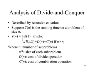
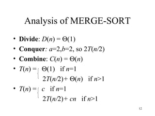
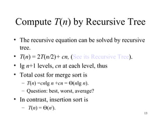
This document discusses algorithm design and analysis. It introduces sorting as an example problem and compares the insertion sort and merge sort algorithms. Insertion sort runs in O(n2) time in the worst case, while merge sort runs in O(nlogn) time. It provides pseudocode for insertion sort and merge sort and analyzes their time complexities. It also covers algorithm analysis techniques like recursion trees and asymptotic notation.

1. 1
Introduction to Algorithm design and analysis
Example: sorting problem.
Input: a sequence of n number <a1, a2, …,an>
Output: a permutation (reordering) <a1', a2', …,an'>
such that a1'≤ a2' ≤ … ≤ an '.
Different sorting algorithms:
Insertion sort and Mergesort.

2. 2
Efficiency comparison of two algorithms
• Suppose n=106
numbers:
– Insertion sort: c1n2
– Merge sort: c2n (lg n)
– Best programmer (c1=2), machine language, one billion/second computer A.
– Bad programmer (c2=50), high-language, ten million/second computer B.
– 2 (106
)2
instructions/109
instructions per second = 2000 seconds.
– 50 (106
lg 106
) instructions/107
instructions per second ≈ 100 seconds.
– Thus, merge sort on B is 20 times faster than insertion sort on A!
– If sorting ten million numbers, 2.3 days VS. 20 minutes.
• Conclusions:
– Algorithms for solving the same problem can differ dramatically in their
efficiency.
– much more significant than the differences due to hardware and software.

3. 3
Algorithm Design and Analysis
• Design an algorithm
– Prove the algorithm is correct.
• Loop invariant.
• Recursive function.
• Formal (mathematical) proof.
• Analyze the algorithm
– Time
• Worse case, best case, average case.
• For some algorithms, worst case occurs often, average case is often roughly as bad as
the worst case. So generally, worse case running time.
– Space
• Sequential and parallel algorithms
– Random-Access-Model (RAM)
– Parallel multi-processor access model: PRAM

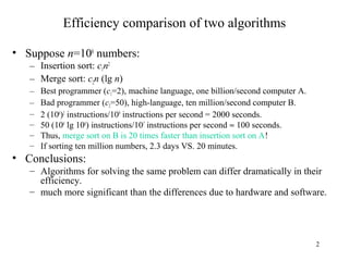
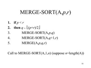
4. 4
Insertion Sort Algorithm (cont.)
INSERTION-SORT(A)
1. for j = 2 to length[A]
2. do key ← A[j]
3. //insert A[j] to sorted sequence A[1..j-1]
4. i ← j-1
5. while i >0 and A[i]>key
6. do A[i+1] ← A[i] //move A[i] one position right
7. i ← i-1
8. A[i+1] ← key

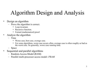
5. 5
Correctness of Insertion Sort Algorithm
• Loop invariant
– At the start of each iteration of the for loop, the
subarray A[1..j-1] contains original A[1..j-1] but in
sorted order.
• Proof:
– Initialization : j=2, A[1..j-1]=A[1..1]=A[1], sorted.
– Maintenance: each iteration maintains loop invariant.
– Termination: j=n+1, so A[1..j-1]=A[1..n] in sorted
order.

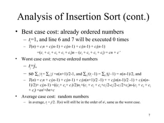
6. 6
Analysis of Insertion Sort
INSERTION-SORT(A) cost times
1. for j = 2 to length[A] c1 n
2. do key ← A[j] c2 n-1
3. //insert A[j] to sorted sequence A[1..j-1] 0 n-1
4. i ← j-1 c4 n-1
5. while i >0 and A[i]>key c5 ∑j=2
n
tj
6. do A[i+1] ← A[i] c6 ∑j=2
n
(tj–1)
7. i ← i-1 c7 ∑j=2
n
(tj–1)
8. A[i+1] ← key c8 n–1
(tj is the number of times the while loop test in line 5 is executed for that value of j)
The total time cost T(n) = sum of cost × times in each line
=c1n + c2(n-1) + c4(n-1) + c5∑j=2
n
tj+ c6∑j=2
n
(tj-1)+ c7∑j=2
n
(tj-1)+ c8(n-1)

7. 7
Analysis of Insertion Sort (cont.)
• Best case cost: already ordered numbers
– tj=1, and line 6 and 7 will be executed 0 times
– T(n) = c1n + c2(n-1) + c4(n-1) + c5(n-1) + c8(n-1)
=(c1 + c2 + c4 + c5 + c8)n – (c2 + c4 + c5 + c8) = cn + c‘
• Worst case cost: reverse ordered numbers
– tj=j,
– so ∑j=2
n
tj= ∑j=2
n
j =n(n+1)/2-1, and ∑j=2
n
(tj–1) = ∑j=2
n
(j–1) = n(n-1)/2, and
– T(n) = c1n + c2(n-1) + c4(n-1) + c5(n(n+1)/2 -1) + + c6(n(n-1)/2 -1) + c7(n(n-
1)/2)+ c8(n-1) =((c5+ c6 + c7)/2)n2 +(c1 + c2 + c4 +c5/2-c6/2-c7/2+c8)n-(c2 + c4 + c5
+ c8) =an2
+bn+c
• Average case cost: random numbers
– in average, tj = j/2. T(n) will still be in the order of n2
, same as the worst case.

8. 8
Merge Sort—divide-and-conquer
• Divide: divide the n-element sequence into
two subproblems of n/2 elements each.
• Conquer: sort the two subsequences
recursively using merge sort. If the length
of a sequence is 1, do nothing since it is
already in order.
• Combine: merge the two sorted
subsequences to produce the sorted answer.

9. 9
Merge Sort –merge function
• Merge is the key operation in merge sort.
• Suppose the (sub)sequence(s) are stored in
the array A. moreover, A[p..q] and
A[q+1..r] are two sorted subsequences.
• MERGE(A,p,q,r) will merge the two
subsequences into sorted sequence A[p..r]
– MERGE(A,p,q,r) takes Θ(r-p+1).

10. 10
MERGE-SORT(A,p,r)
1. if p < r
2. then q ← (p+r)/2
3. MERGE-SORT(A,p,q)
4. MERGE-SORT(A,q+1,r)
5. MERGE(A,p,q,r)
Call to MERGE-SORT(A,1,n) (suppose n=length(A))

11. 11
Analysis of Divide-and-Conquer
• Described by recursive equation
• Suppose T(n) is the running time on a problem of
size n.
• T(n) = Θ(1) if n≤nc
aT(n/b)+D(n)+C(n) if n> nc
Where a: number of subproblems
n/b: size of each subproblem
D(n): cost of divide operation
C(n): cost of combination operation

12. 12
Analysis of MERGE-SORT
• Divide: D(n) = Θ(1)
• Conquer: a=2,b=2, so 2T(n/2)
• Combine: C(n) = Θ(n)
• T(n) = Θ(1) if n=1
2T(n/2)+ Θ(n) if n>1
• T(n) = c if n=1
2T(n/2)+ cn if n>1

13. 13
Compute T(n) by Recursive Tree
• The recursive equation can be solved by recursive
tree.
• T(n) = 2T(n/2)+ cn, (See its Recursive Tree).
• lg n+1 levels, cn at each level, thus
• Total cost for merge sort is
– T(n) =cnlg n +cn = Θ(nlg n).
– Question: best, worst, average?
• In contrast, insertion sort is
– T(n) = Θ(n2
).

14. 14
Recursion tree of T(n)=2T(n/2)+cn

15. 15
Order of growth
• Lower order item(s) are ignored, just keep the
highest order item.
• The constant coefficient(s) are ignored.
• The rate of growth, or the order of growth,
possesses the highest significance.
• Use Θ(n2
) to represent the worst case running time
for insertion sort.
• Typical order of growth: Θ(1), Θ(lg n),
Θ(√n),Θ(n), Θ(nlg n), Θ(n2
), Θ(n3
), Θ(2n
), Θ(n!)
• Asymptotic notations: Θ, O, Ω, o, ω.

16. 16
f(n) = Θ(g(n))
n
n0
c1g(n)
c2g(n)
f(n)
f(n) = O(g(n))
n
n0
f(n)
cg(n)
f(n) = Ω(g(n))
nn0
cg(n)
f(n)
There exist positive constants c1 and c2
such that there is a positive constant n0
such that …
There exist positive constants c
such that there is a positive constant n0
such that …
There exist positive constants c
such that there is a positive constant n0
such that …

17. Prove f(n)=an2
+bn+c=Θ(n2
)
• a, b, c are constants and a>0.
• Find c1, and c2 (and n0) such that
– c1n2
≤f(n) ≤c2n2
for all n≥ n0.
• It turns out: c1=a/4, c2=7a/4 and
– n0= 2⋅max(|b|/a, sqrt(|c|/a))
• Here we also can see that lower terms and
constant coefficient can be ignored.
• How about f(n)=an3
+bn2
+cn+d? 17

18. 18
o-notation
• For a given function g(n),
– o(g(n))={f(n): for any positive constant c,there exists a
positive n0 such that 0≤ f(n) ≤ cg(n) for all n≥ n0}
– Write f(n) ∈ o(g(n)), or simply f(n) = o(g(n)).
2g(n)
f(n) = o(g(n))
nn0
g(n)
f(n)
1/2g(n)
n0 n0

19. 19
Notes on o-notation
• O-notation may or may not be asymptotically tight
for upper bound.
– 2n2
= O(n2
) is tight, but 2n = O(n2
) is not tight.
• o-notition is used to denote an upper bound that is
not tight.
– 2n = o(n2
), but 2n2
≠ o(n2
).
• Difference: for some positive constant c in O-
notation, but all positive constants c in o-notation.
• In o-notation, f(n) becomes insignificant relative to
g(n) as n approaches infinitely: i.e.,
– lim = 0.f(n)
g(n)n→∝

20. 20
ω-notation
• For a given function g(n),
ω(g(n))={f(n): for any positive constant c, there exists a
positive n0 such that 0 ≤ cg(n) ≤ f(n) for all n≥ n0}
– Write f(n) ∈ ω(g(n)), or simply f(n) = ω(g(n)).
∀ ω-notation, similar to o-notation, denotes lower
bound that is not asymptotically tight.
– n2
/2 = ω(n), but n2
/2 ≠ ω(n2
)
• f(n) = ω(g(n)) if and only if g(n)=o(f(n)).
• lim = ∝
f(n)
g(n)n→∝

21. 21
Techniques for Algorithm Design and Analysis
• Data structure: the way to store and organize data.
– Disjoint sets
– Balanced search trees (red-black tree, AVL tree, 2-3 tree).
• Design techniques:
– divide-and-conquer, dynamic programming, prune-and-search,
laze evaluation, linear programming, …
• Analysis techniques:
– Analysis: recurrence, decision tree, adversary argument,
amortized analysis,…

22. 22
NP-complete problem
• Hard problem:
– Most problems discussed are efficient (poly time)
– An interesting set of hard problems: NP-complete.
• Why interesting:
– Not known whether efficient algorithms exist for them.
– If exist for one, then exist for all.
– A small change may cause big change.
• Why important:
– Arise surprisingly often in real world.
– Not waste time on trying to find an efficient algorithm to get best
solution, instead find approximate or near-optimal solution.
• Example: traveling-salesman problem.