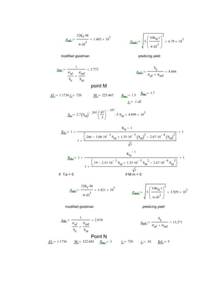
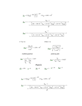
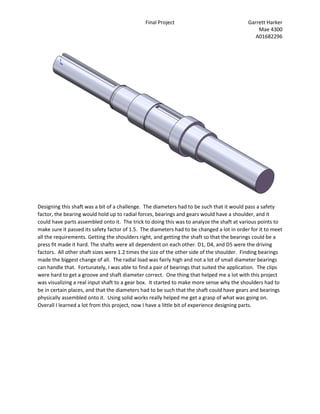
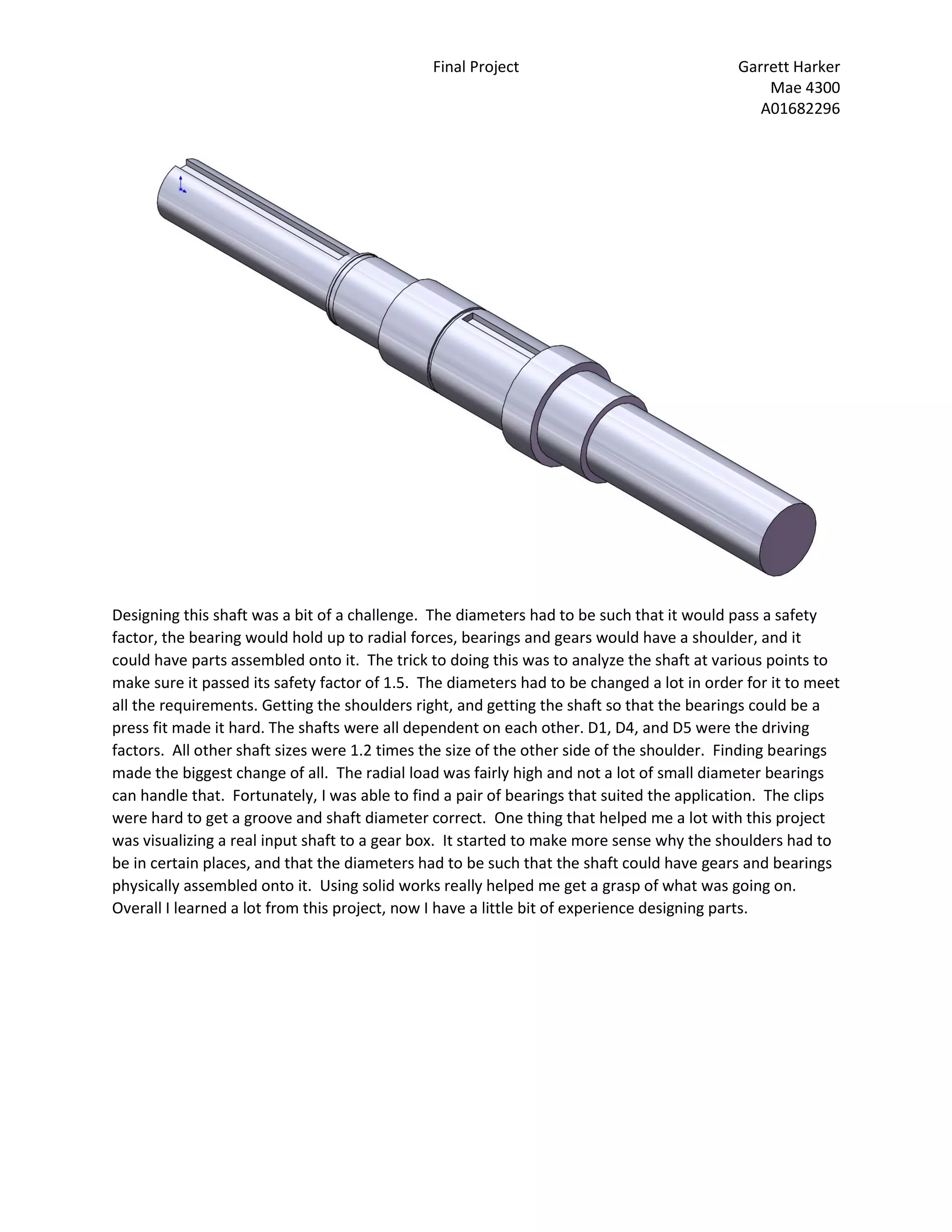
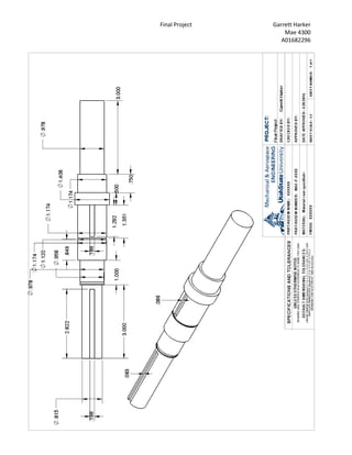
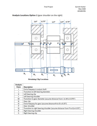
The document describes the challenges of designing a shaft to meet several requirements. The shaft diameters had to pass a safety factor test, support radial forces on bearings, and allow bearings and gears to mount onto the shaft. Analyzing the shaft at different points ensured it met the 1.5 safety factor. Diameters and shoulders were adjusted to satisfy all criteria. Visualizing a real input shaft helped understand design constraints. Solidworks modeling aided comprehension. The project provided shaft design experience.

1. Final Project Garrett Harker
Mae 4300
A01682296
Designing this shaft was a bit of a challenge. The diameters had to be such that it would pass a safety
factor, the bearing would hold up to radial forces, bearings and gears would have a shoulder, and it
could have parts assembled onto it. The trick to doing this was to analyze the shaft at various points to
make sure it passed its safety factor of 1.5. The diameters had to be changed a lot in order for it to meet
all the requirements. Getting the shoulders right, and getting the shaft so that the bearings could be a
press fit made it hard. The shafts were all dependent on each other. D1, D4, and D5 were the driving
factors. All other shaft sizes were 1.2 times the size of the other side of the shoulder. Finding bearings
made the biggest change of all. The radial load was fairly high and not a lot of small diameter bearings
can handle that. Fortunately, I was able to find a pair of bearings that suited the application. The clips
were hard to get a groove and shaft diameter correct. One thing that helped me a lot with this project
was visualizing a real input shaft to a gear box. It started to make more sense why the shoulders had to
be in certain places, and that the diameters had to be such that the shaft could have gears and bearings
physically assembled onto it. Using solid works really helped me get a grasp of what was going on.
Overall I learned a lot from this project, now I have a little bit of experience designing parts.

2. Final Project Garrett Harker
Mae 4300
A01682296

3. Final Project Garrett Harker
Mae 4300
A01682296

4. Final Project Garrett Harker
Mae 4300
A01682296

5. Math Cad Calculations
Functions used to automate the computations:
Combinind Eq. 6-19 and 6-20: Sef Sut d  2.7
Sut
ksi






0.265

d
in
0.3








0.107
 0.5 Sut
Using Eq. 6-33, 6-34, 6-35, and 6-36, we get the following functions to compute Kf and Kfs.
Kff Sut r Kt  1
Kt 1
1
0.246 3.08 10
3

Sut
ksi
 1.51 10
5

Sut
ksi






2
 2.67 10
8

Sut
ksi






3







in
r


Kfs Sut r Kts  1
Kts 1
1
0.19 2.51 10
3

Sut
ksi
 1.35 10
5

Sut
ksi






2
 2.67 10
8

Sut
ksi






3







in
r


Eq 7-5 assuming Ta = 0: σaf Kf M D 
32 Kf M
π D
3


Eq 7-6 assuming Mm = 0: σmf Kfs T D  3
16 Kfs T
π D
3







2

Eq. 6-46 for fatigue safety factor using modified Goodman nff σa σm Se Sut 
1
σa
Se
σm
Sut


Eq. 6-49 for predicting yield (conservative approach): nyf Sy σ'a σ'm 
Sy
σ'a σ'm

ratedLoad af FD RD a b x0 θ xD  af FD
xD
x0 θ x0  ln
1
RD












1
b













1
a

Eq. 11-6 for C10
bearing loads

6. Parameters
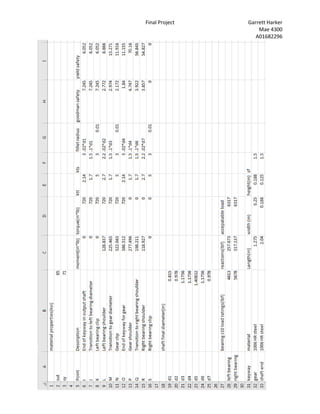
Ti 60 ω 1750 W23 540 Pmin 5.76
wface 1.5 J .27 YN .88
σ 13040 Kv 1.37 Km 1.19 σc 94000 L2 1.26 10
9

gear design is all from Mechanical Engineering Design 10th
d2 2.667 d3 12 d4 2.667 d5 12
n3 72
n2 16 n4 16 n5 72 p 20
t2 60 t3 270 t4 270 t5 1215.5
ω2 1750 ω5 86.42
w23t 540
w45t 2431
w23r 197
w45r 885
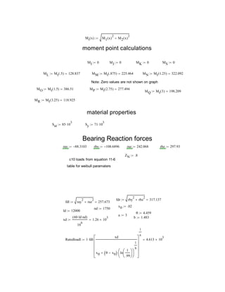
material properties
sae 1040 cd 85ksitensile 71 ksi yield
sut 85 10
3
 sy 71 10
3

Reaction forces calculation and matrix
ray 0 rby 0 raz 0 rbz 0
la 2 lab 3.625
Reaction matrix
ray rby 197
raz rbz 540
1
0
0
0
1
0
0
3.625
0
1
0
0
0
1
3.625
0
197
540
1080
394












3.625 rbz 1080
3.625rb 394
Ray 88.3103 Rby 108.6896 Raz 242.068 Rbz 297.931
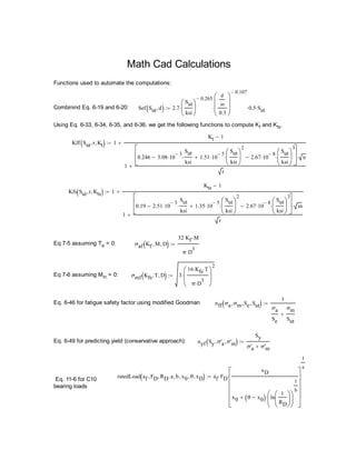
moment diagrams
M1 x( ) Raz x( ) x 2if
Raz 2 Rbz x 2( )[ ] x 2if


7. 0 1 2 3
100
0
100
200
300
400
500
M1 x( )
x
M2 x( ) Ray x( ) x 2if
Ray 2 Rby x 2( )[ ] x 2if

0 1 2 3
200
150
100
50
0
M2 x( )
x

8. Mt x( ) M1 x( )
2
M2 x( )
2

moment point calculations
MI 0 MJ 0 MK 0 MS 0
ML Mt .5( ) 128.837 MM Mt .875( ) 225.464 MN Mt 1.25( ) 322.092
Note: Zero values are not shown on graph
MO Mt 1.5( ) 386.51 MP Mt 2.75( ) 277.494
MQ Mt 3( ) 198.209
MR Mt 3.25( ) 118.925
material properties
Sut 85 10
3
 Sy 71 10
3

Bearing Reaction forces
ray 88.3103 rby 108.6896 raz 242.068 rbz 297.93
ZN .8
c10 loads from equation 11-6
table for weibull paramaters
fdr rby
2
rbz
2
 317.137
fdl ray
2
raz
2
 257.673
x0 .02
nd 1750
ld 12000
θ 4.459
a 3
b 1.483
xd
60 ld nd( )
10
6
1.26 10
3

Ratedloadl 1 fdl
xd
x0 θ x0  ln
1
.99












1
b













1
a
 4.613 10
3


9. Ratedloadr 1 fdr
xd
x0 θ x0  ln
1
.99












1
b













1
a
 5.678 10
3

shaft point analysis
Point I
Ktt 2.14
d1 .815 Kts 3 M 0 r .02 d1 t 720
Se 2.7 Sut 
.265 d1
.3






.107
 .5 Sut 5.093 10
3

Kf 1
Ktt 1
1
.246 3.08 10
3
 Sut 1.35 10
5
 Sut 2
 2.67 10
8
 Sut 3




r

 1
if T.a = 0 if M.m = 0
Kfs 1
Kts
1
1
.19 2.51 10
3
 Sut 1.35 10
5
 Sut
2
 2.67 10
8
 Sut
3




r

 1
σaf
32Kf M
π d1( )
3

0
σmf 3
16Kfs t
π d1
3







2
 1.173 10
4

modified goodman
predicing yield

10. nff
1
σaf
Se
σmf
Sut

7.245
nyf
Sy
σaf σmf
6.052
point j
r .1 d1
d1 .815 Kts 1.5 M 0 t 720 Ktt 1.7
Se 2.7 Sut 
.265 d1
.3






.107
 .5 Sut 5.093 10
3

Kf 1
Ktt 1
1
.246 3.08 10
3
 Sut 1.35 10
5
 Sut 2
 2.67 10
8
 Sut 3




r

 1
if T.a = 0 if M.m = 0
Kfs 1
Kts
1
1
.19 2.51 10
3
 Sut 1.35 10
5
 Sut
2
 2.67 10
8
 Sut
3




r

 1
σaf
32Kf M
π d1
3

0
σmf 3
16Kfs t
π d1
3







2
 1.173 10
4

modified goodman predicing yield
nff
1
σaf
Se
σmf
Sut

7.245
nyf
Sy
σaf σmf
6.052
point k
Ktt 5
r .01 d1 .815 Kts 3 M 0 t 720
Se 2.7 Sut 
.265 d1
.3






.107
 .5 Sut 5.093 10
3


11. Kf 1
Ktt 1
1
.246 3.08 10
3
 Sut 1.35 10
5
 Sut 2
 2.67 10
8
 Sut 3




r

 1
if T.a = 0 if M.m = 0
Kfs 1
Kts
1
1
.19 2.51 10
3
 Sut 1.35 10
5
 Sut
2
 2.67 10
8
 Sut
3




r

 1
σaf
32Kf M
π d1
3

0
σmf 3
16Kfs t
π d1
3







2
 1.173 10
4

modified goodman predicing yield
nff
1
σaf
Se
σmf
Sut

7.245
nyf
Sy
σaf σmf
6.052
point L
Ktt 2.7
d2 .978 t 720 M 128.837 Kts 2.2
r .02 d2
Se 2.7 Sut 
.265 d2
.3






.107
 .5 Sut 4.995 10
3

Kf 1
Ktt 1
1
.246 3.08 10
3
 Sut 1.35 10
5
 Sut 2
 2.67 10
8
 Sut 3




r

 1
Kfs 1
Kts
1
1
.19 2.51 10
3
 Sut 1.35 10
5
 Sut
2
 2.67 10
8
 Sut
3




r

 1
if T.a = 0 if M.m = 0

12. σaf
32Kf M
π d2
3

1.403 10
3

σmf 3
16Kfs t
π d2
3







2
 6.79 10
3

modified goodman predicing yield
nff
1
σaf
Se
σmf
Sut

2.772
nyf
Sy
σaf σmf
8.666
point M
Ktt 1.7
d3 1.1736 t 720 M 225.465 Kts 1.5
r .1 d2
Se 2.7 Sut 
.265 d3
.3






.107
 .5 Sut 4.899 10
3

Kf 1
Ktt 1
1
.246 3.08 10
3
 Sut 1.35 10
5
 Sut 2
 2.67 10
8
 Sut 3




r

 1
Kfs 1
Kts
1
1
.19 2.51 10
3
 Sut 1.35 10
5
 Sut
2
 2.67 10
8
 Sut
3




r

 1
if T.a = 0 if M.m = 0
σaf
32Kf M
π d3
3

1.421 10
3

σmf 3
16Kfs t
π d3
3







2
 3.929 10
3

modified goodman predicing yield
nff
1
σaf
Se
σmf
Sut

2.974
nyf
Sy
σaf σmf
13.271
Point N
d3 1.1736 M 322.043 Kts 3 t 720 r .01 Ktt 5

13. Se 2.7 Sut 
.265 d3
.3






.107
 .5 Sut 4.899 10
3

Kf 1
Ktt 1
1
.246 3.08 10
3
 Sut 1.35 10
5
 Sut 2
 2.67 10
8
 Sut 3




r

 1
Kfs 1
Kts
1
1
.19 2.51 10
3
 Sut 1.35 10
5
 Sut
2
 2.67 10
8
 Sut
3




r

 1
if T.a = 0 if M.m = 0
σaf
32Kf M
π d3
3

2.029 10
3

σmf 3
16Kfs t
π d3
3







2
 3.929 10
3

modified goodman predicing yield
nff
1
σaf
Se
σmf
Sut

2.172
nyf
Sy
σaf σmf
11.916
Point O
Ktt 2.14
d4 d3 1.174 t 720 M 386.512 Kts 3
r .02 d4
Se 2.7 Sut 
.265 d4
.3






.107
 .5 Sut 4.899 10
3

Kf 1
Ktt 1
1
.246 3.08 10
3
 Sut 1.35 10
5
 Sut 2
 2.67 10
8
 Sut 3




r

 1

14. Kfs 1
Kts
1
1
.19 2.51 10
3
 Sut 1.35 10
5
 Sut
2
 2.67 10
8
 Sut
3




r

 1
if T.a = 0 if M.m = 0
σaf
32Kf M
π d4
3

2.436 10
3

σmf 3
16Kfs t
π d4
3







2
 3.929 10
3

modified goodman predicing yield
nff
1
σaf
Se
σmf
Sut

1.84
nyf
Sy
σaf σmf
11.155
Point P
Ktt 1.7
d5 1.4083 t 0 M 277.496 Kts 1.5 r .1 d5
Se 2.7 Sut 
.265 d5
.3






.107
 .5 Sut 4.804 10
3

Kf 1
Ktt 1
1
.246 3.08 10
3
 Sut 1.35 10
5
 Sut 2
 2.67 10
8
 Sut 3




r

 1
Kfs 1
Kts
1
1
.19 2.51 10
3
 Sut 1.35 10
5
 Sut
2
 2.67 10
8
 Sut
3




r

 1
if T.a = 0 if M.m = 0
σaf
32Kf M
π d5
3

1.012 10
3

σmf 3
16Kfs t
π d5
3







2
 0
modified goodman predicing yield

15. nff
1
σaf
Se
σmf
Sut

4.747
nyf
Sy
σaf σmf
70.16
Point Q
Ktt 1.7
d6 1.1736 M 198.211 t 0 Kts 1.5
r .1 d6
Se 2.7 Sut 
.265 d6
.3






.107
 .5 Sut 4.899 10
3

Kf 1
Ktt 1
1
.246 3.08 10
3
 Sut 1.35 10
5
 Sut 2
 2.67 10
8
 Sut 3




r

 1
Kfs 1
Kts
1
1
.19 2.51 10
3
 Sut 1.35 10
5
 Sut
2
 2.67 10
8
 Sut
3




r

 1
if T.a = 0 if M.m = 0
σaf
32Kf M
π d6
3

1.249 10
3

σmf 3
16Kfs t
π d6
3







2
 0
modified goodman predicing yield
nff
1
σaf
Se
σmf
Sut

3.922
nyf
Sy
σaf σmf
56.845
Point R
Ktt 2.7
d7 .978 M 118.927 t 0 Kts 2.2
r 02 d7

16. Se 2.7 Sut 
.265 d7
.3






.107
 .5 Sut 4.995 10
3

Kf 1
Ktt 1
1
.246 3.08 10
3
 Sut 1.35 10
5
 Sut 2
 2.67 10
8
 Sut 3




r

 1
Kfs 1
Kts
1
1
.19 2.51 10
3
 Sut 1.35 10
5
 Sut
2
 2.67 10
8
 Sut
3




r

 1
if T.a = 0 if M.m = 0
σaf
32Kf M
π d7
3

1.295 10
3

σmf 3
16Kfs t
π d7
3







2
 0
modified goodman predicing yield
nff
1
σaf
Se
σmf
Sut

3.857
nyf
Sy
σaf σmf
54.827
Point S
r .01 Ktt 5
d7 .978 t 0 M 0 Kts 3
Se 2.7 Sut 
.265 d7
.3






.107
 .5 Sut 4.995 10
3

Kf 1
Ktt 1
1
.246 3.08 10
3
 Sut 1.35 10
5
 Sut 2
 2.67 10
8
 Sut 3




r

 1

17. Kfs 1
Kts
1
1
.19 2.51 10
3
 Sut 1.35 10
5
 Sut
2
 2.67 10
8
 Sut
3




r

 1
if T.a = 0 if M.m = 0
σaf
32Kf M
π d7
3

0
σmf 3
16Kfs t
π d7
3







2
 0
modified goodman predicing yield
nff
1
σaf
Se
σmf
Sut


σaf
Se
σmf
Sut

nyf
Sy
σaf σmf

σaf σmf
since there is no stress there is no safety factor
Key ways
table 7-6 for key parameters
sy 24
sf 1.5
Key material 1006 HR
d4 1.174
sykey
sy
3
13.856
table 7-6
gear keyway
wg
1
4
0.25 hg
3
16
0.188 dg
3
32
0.094
fg
720 12( )
d4
2
1.472 10
4


18. crushing
cg
2 fg sf( )
wg sykey 10000
1.275
shear
sg
fg sf
wg sykey 10000
0.638
end of shaft key way
d7 0.978
ds
1
16
0.063
fs
720 12
d7
2
1.767 10
4

hs
1
8
0.125
crushing
ws
3
16
0.188
cs
2 fs sf
ws sykey 10000
2.04
shear
ss
fs sf
ws sykey 10000
1.02

19. Final Project Garrett Harker
Mae 4300
A01682296
Bearings
http://www.globalspec.com/specsearch/partspecs?partId={7B589298-8679-4CE6-9AA3-
6FF2313DAABE}&comp=50&vid=335701&sqid=16701685
Rings
End of shaft

20. Final Project Garrett Harker
Mae 4300
A01682296
http://www.globalspec.com/specsearch/partspecs?partId={BE29DFD9-8364-4F54-93CF-
1D584E194E66}&comp=287&vid=132871&sqid=16703112
gear ring
http://www.globalspec.com/specsearch/partspecs?partId={1281AAB0-9E11-43D0-8820-
12D7F406BF47}&comp=287&vid=132871&sqid=16703581

21. Final Project Garrett Harker
Mae 4300
A01682296