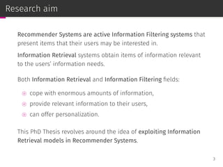
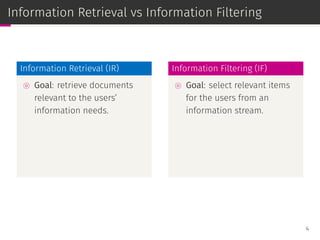
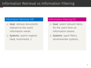
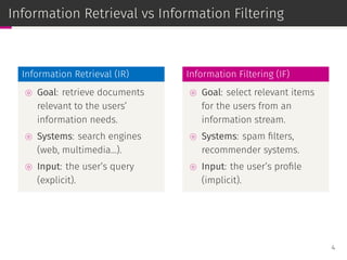
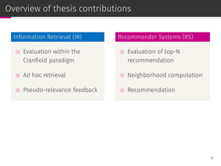
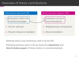
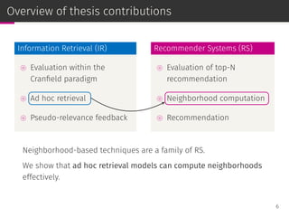
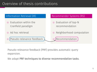
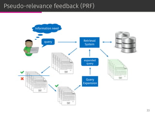
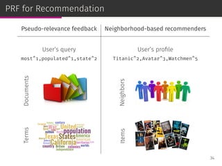
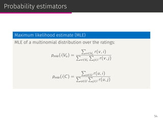
This PhD thesis by Daniel Valcarce explores the intersection of information retrieval models and recommender systems, emphasizing their shared goal of providing relevant information to users. The work includes evaluations of various recommendation techniques and metrics, highlighting robust methods for assessing the effectiveness of recommendations. Key contributions involve adapting information retrieval techniques for enhancing recommender systems, particularly through pseudo-relevance feedback and neighborhood-based approaches.


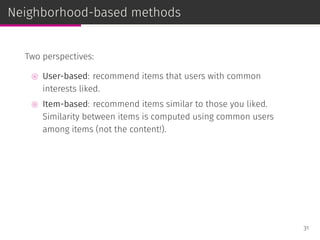


![Relevance models
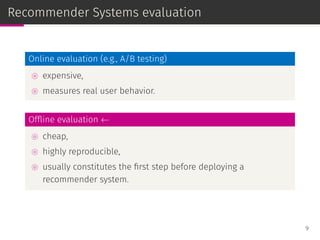
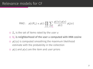
Relevance-based language models or, simply, relevance models (RM)
are state-of-the-art PRF methods [Lavrenko & Croft, SIGIR ’01]:
⊚ RM1: i.i.d. sampling,
⊚ RM2: conditional sampling.
36](https://image.slidesharecdn.com/slides-190509153630/85/Information-Retrieval-Models-for-Recommender-Systems-PhD-slides-63-320.jpg)
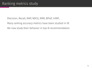
![Relevance models
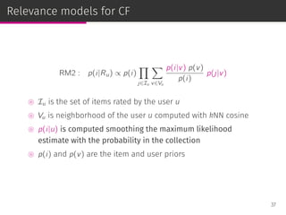
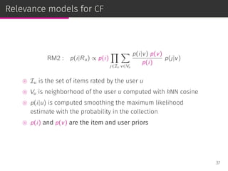
Relevance-based language models or, simply, relevance models (RM)
are state-of-the-art PRF methods [Lavrenko & Croft, SIGIR ’01]:
⊚ RM1: i.i.d. sampling,
⊚ RM2: conditional sampling.
RM has been adapted to user-based CF [Parapar et al., IPM ’13].
36](https://image.slidesharecdn.com/slides-190509153630/85/Information-Retrieval-Models-for-Recommender-Systems-PhD-slides-64-320.jpg)
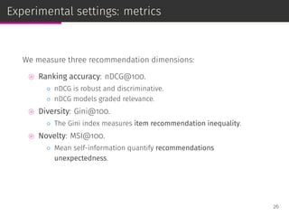
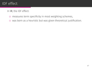
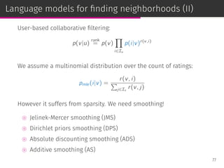
![Why use smoothing?
In IR [Zhai & Lafferty, TOIS 2004], smoothing provides:
⊚ a way to deal with data sparsity,
⊚ inverse document frequency (IDF) effect,
⊚ document length normalization.
39](https://image.slidesharecdn.com/slides-190509153630/85/Information-Retrieval-Models-for-Recommender-Systems-PhD-slides-71-320.jpg)
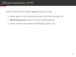
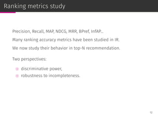
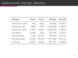
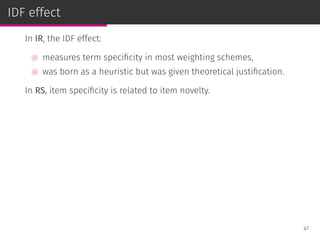
![Why use smoothing?
In IR [Zhai & Lafferty, TOIS 2004], smoothing provides:
⊚ a way to deal with data sparsity,
⊚ inverse document frequency (IDF) effect,
⊚ document length normalization.
In RS, we have the same problems:
⊚ data sparsity,
⊚ item popularity/specificity,
⊚ user profiles with different sizes.
39](https://image.slidesharecdn.com/slides-190509153630/85/Information-Retrieval-Models-for-Recommender-Systems-PhD-slides-72-320.jpg)
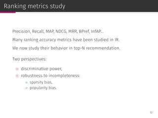
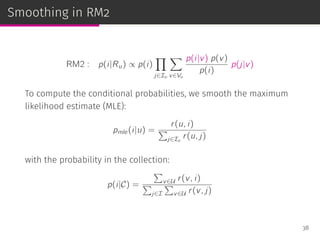
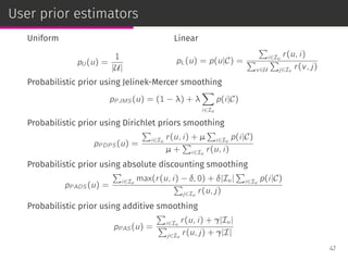
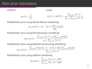
![Smoothing techniques
Jelinek-Mercer smoothing (JMS): linear interpolation controlled by λ.
pλ(i|u) = (1 − λ) pmle(i|u) + λ p(i|C)
Dirichlet priors smoothing (DPS): Bayesian analysis with parameter µ.
pµ(i|u) =
r(u, i) + µ p(i|C)
µ +
∑
j∈Iu
r(u, j)
Absolute discounting smoothing (ADS): subtract a constant δ.
pδ(i|u) =
max[r(u, i) − δ, 0] + δ |Iu|p(i|C)
∑
j∈Iu
r(u, j)
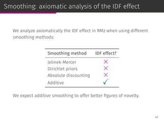
Additive smoothing (AS): increase all the ratings by γ > 0.
pγ(i|u) =
r(u, i) + γ
∑
j∈Iu
r(u, j) + γ |I|
40](https://image.slidesharecdn.com/slides-190509153630/85/Information-Retrieval-Models-for-Recommender-Systems-PhD-slides-73-320.jpg)

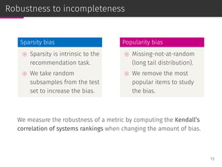
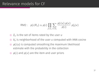
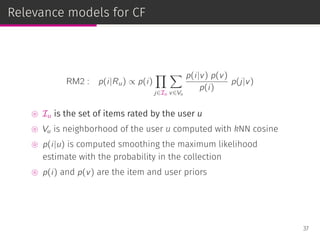
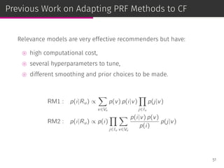
![Priors in RM2
RM2 : p(i|Ru) ∝ p(i)
∏
j∈Iu
∑
v∈Vu
p(i|v) p(v)
p(i)
p(j|v)
p(i) and p(v) are the item and user priors:
⊚ enable to introduce a priori information into the model,
⊚ provide a principled way of modeling business rules,
⊚ similar to document priors used in IR such as:
◦ linear document length prior [Kraaij et al., SIGIR ’02],
◦ probabilistic document length prior [Blanco & Barreiro, ECIR ’08].
46](https://image.slidesharecdn.com/slides-190509153630/85/Information-Retrieval-Models-for-Recommender-Systems-PhD-slides-83-320.jpg)

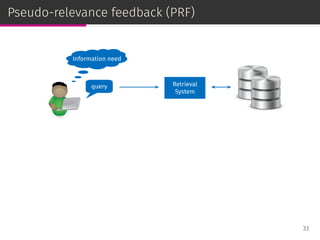
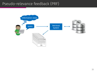
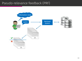
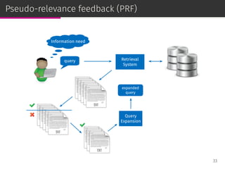
![Popular approaches to pseudo-relevance feedback
⊚ Relevance models
[Lavrenko & Croft, SIGIR ’01]
⊚ Scoring functions based on the Rocchio framework
[Rocchio, 1971; Carpineto et al., ACM TOIS ’01]
⊚ Divergence minimization model
[Zhai & Lafferty, SIGIR ’06]
⊚ Mixture models
[Tao & Zhai, SIGIR ’06]
52](https://image.slidesharecdn.com/slides-190509153630/85/Information-Retrieval-Models-for-Recommender-Systems-PhD-slides-89-320.jpg)
![Popular approaches to pseudo-relevance feedback
⊚ Relevance models
[Lavrenko & Croft, SIGIR ’01]
⊚ Scoring functions based on the Rocchio framework
[Rocchio, 1971; Carpineto et al., ACM TOIS ’01]
⊚ Divergence minimization model
[Zhai & Lafferty, SIGIR ’06]
⊚ Mixture models
[Tao & Zhai, SIGIR ’06]
52](https://image.slidesharecdn.com/slides-190509153630/85/Information-Retrieval-Models-for-Recommender-Systems-PhD-slides-90-320.jpg)
![Scoring functions from Rocchio framework
Rocchio Weights (RW)
pRW (i|u) =
∑
v∈Vu
r(v, i)
|Vu|
Robertson Selection Value (RSV)
pRSV (i|u) = p(i|Vu)
∑
v∈Vu
r(v, i)
|Vu|
CHI2
pCHI2 (i|u) =
[
p(i|Vu) − p(i|C)
]2
p(i|C)
Kullback–Leibler Divergence (KLD)
pKLD(i|u) = p(i|Vu) log
p(i|Vu)
p(i|C)
53](https://image.slidesharecdn.com/slides-190509153630/85/Information-Retrieval-Models-for-Recommender-Systems-PhD-slides-91-320.jpg)
![Scoring functions from Rocchio framework
Rocchio Weights (RW)
pRW (i|u) =
∑
v∈Vu
r(v, i)
|Vu|
Robertson Selection Value (RSV)
pRSV (i|u) = p(i|Vu)
∑
v∈Vu
r(v, i)
|Vu|
CHI2
pCHI2 (i|u) =
[
p(i|Vu) − p(i|C)
]2
p(i|C)
Kullback–Leibler Divergence (KLD)
pKLD(i|u) = p(i|Vu) log
p(i|Vu)
p(i|C)
53](https://image.slidesharecdn.com/slides-190509153630/85/Information-Retrieval-Models-for-Recommender-Systems-PhD-slides-92-320.jpg)
![Scoring functions from Rocchio framework
Rocchio Weights (RW)
pRW (i|u) =
∑
v∈Vu
r(v, i)
|Vu|
Robertson Selection Value (RSV)
pRSV (i|u) = p(i|Vu)
∑
v∈Vu
r(v, i)
|Vu|
CHI2
pCHI2 (i|u) =
[
p(i|Vu) − p(i|C)
]2
p(i|C)
Kullback–Leibler Divergence (KLD)
pKLD(i|u) = p(i|Vu) log
p(i|Vu)
p(i|C)
53](https://image.slidesharecdn.com/slides-190509153630/85/Information-Retrieval-Models-for-Recommender-Systems-PhD-slides-93-320.jpg)

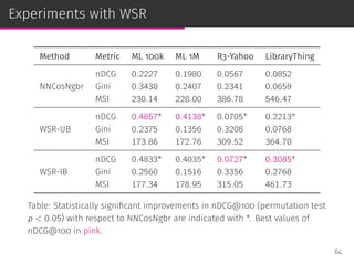
![Weighted sum recommender (WSR)
NNCosNgbr [Cremonesi et al., RecSys ’10]
We bias the MLE to perform neighborhood size normalization:
ˆru,i = bu,i +
∑
j∈Ji
shrunk_cosine (i, j) (r(u, j)−bu,i )
63](https://image.slidesharecdn.com/slides-190509153630/85/Information-Retrieval-Models-for-Recommender-Systems-PhD-slides-104-320.jpg)
![Weighted sum recommender (WSR)
NNCosNgbr [Cremonesi et al., RecSys ’10]
We bias the MLE to perform neighborhood size normalization:
ˆru,i = bu,i +
∑
j∈Ji
shrunk_cosine (i, j) (r(u, j)−bu,i )
Item-based weighted sum recommender (WSR-IB)
ˆru,i =
∑
j∈Ji
cos (i, j) r(u, j)
User-based weighted sum recommender (WSR-UB)
ˆru,i =
∑
v∈Vu
cos (u, v) r(v, i)
63](https://image.slidesharecdn.com/slides-190509153630/85/Information-Retrieval-Models-for-Recommender-Systems-PhD-slides-105-320.jpg)


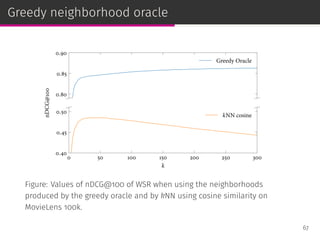
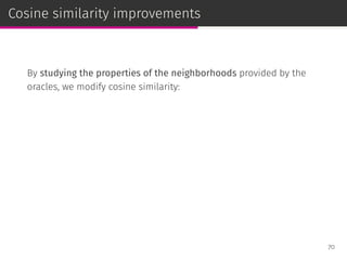
![Cosine similarity improvements
By studying the properties of the neighborhoods provided by the
oracles, we modify cosine similarity:
⊚ We penalize the cosine similarity to add user profile size
normalization.
◦ Similar to the pivoted document length normalization in IR
[Singhal et al., SIGIR ’96].
70](https://image.slidesharecdn.com/slides-190509153630/85/Information-Retrieval-Models-for-Recommender-Systems-PhD-slides-115-320.jpg)
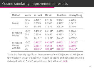
![Cosine similarity improvements
By studying the properties of the neighborhoods provided by the
oracles, we modify cosine similarity:
⊚ We penalize the cosine similarity to add user profile size
normalization.
◦ Similar to the pivoted document length normalization in IR
[Singhal et al., SIGIR ’96].
⊚ We add the IDF effect to cosine similarity to increase the user
profile overlap of the neighbors.
◦ The IDF is a fundamental term specificity measure in IR.
70](https://image.slidesharecdn.com/slides-190509153630/85/Information-Retrieval-Models-for-Recommender-Systems-PhD-slides-116-320.jpg)


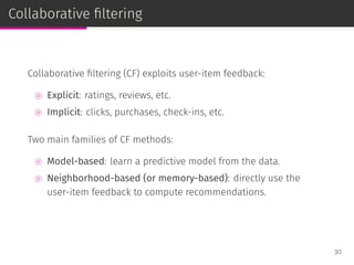
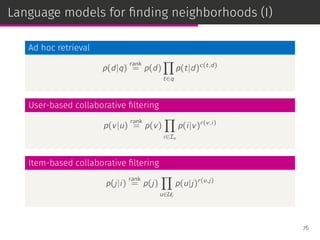
![Language models
Statistical language models are a state-of-the-art ad hoc retrieval
framework [Ponte & Croft, SIGIR ’98].
Documents are ranked according to their posterior probability given
the query:
p(d|q) =
p(q|d) p(d)
p(q)
rank
= p(q|d) p(d)
75](https://image.slidesharecdn.com/slides-190509153630/85/Information-Retrieval-Models-for-Recommender-Systems-PhD-slides-124-320.jpg)
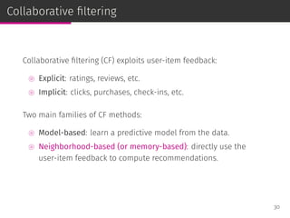
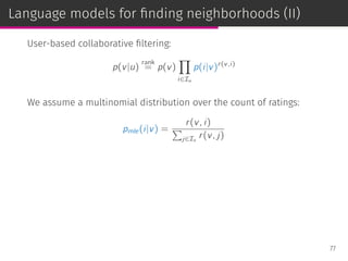
![Language models
Statistical language models are a state-of-the-art ad hoc retrieval
framework [Ponte & Croft, SIGIR ’98].
Documents are ranked according to their posterior probability given
the query:
p(d|q) =
p(q|d) p(d)
p(q)
rank
= p(q|d) p(d)
The query likelihood, p(q|d), is based on a unigram model:
p(q|d) =
∏
t∈q
p(t|d)c(t,d)
75](https://image.slidesharecdn.com/slides-190509153630/85/Information-Retrieval-Models-for-Recommender-Systems-PhD-slides-125-320.jpg)
![Language models
Statistical language models are a state-of-the-art ad hoc retrieval
framework [Ponte & Croft, SIGIR ’98].
Documents are ranked according to their posterior probability given
the query:
p(d|q) =
p(q|d) p(d)
p(q)
rank
= p(q|d) p(d)
The query likelihood, p(q|d), is based on a unigram model:
p(q|d) =
∏
t∈q
p(t|d)c(t,d)
The document prior, p(d), is usually considered uniform.
75](https://image.slidesharecdn.com/slides-190509153630/85/Information-Retrieval-Models-for-Recommender-Systems-PhD-slides-126-320.jpg)


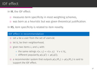
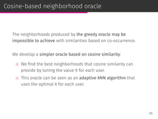
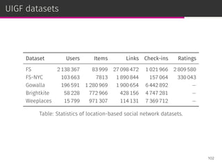
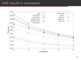
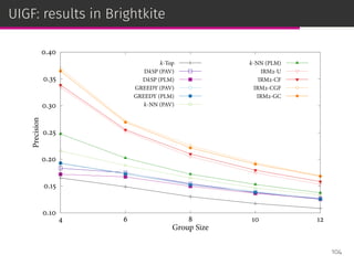
![User-item group formation
The user-item group formation (UIGF) problem aims to find the best
companions for a given item and a target user [Brilhante et al.,
ICMDM ’16].
98](https://image.slidesharecdn.com/slides-190509153630/85/Information-Retrieval-Models-for-Recommender-Systems-PhD-slides-156-320.jpg)
![User-item group formation
The user-item group formation (UIGF) problem aims to find the best
companions for a given item and a target user [Brilhante et al.,
ICMDM ’16].
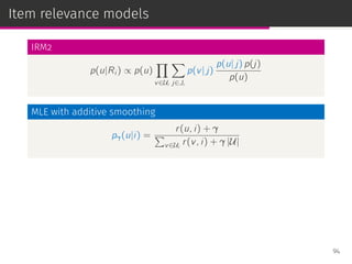
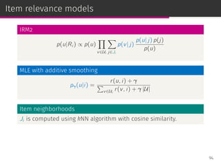
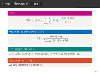
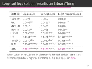
IRM2:
⊚ estimates the relevance of a user given an item;
⊚ deals with long tail item liquidation with uniform priors.
98](https://image.slidesharecdn.com/slides-190509153630/85/Information-Retrieval-Models-for-Recommender-Systems-PhD-slides-157-320.jpg)
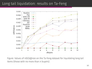
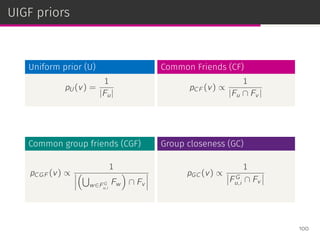
![User-item group formation
The user-item group formation (UIGF) problem aims to find the best
companions for a given item and a target user [Brilhante et al.,
ICMDM ’16].
IRM2:
⊚ estimates the relevance of a user given an item;
⊚ deals with long tail item liquidation with uniform priors.
We can model the user relationships with different priors estimators.
98](https://image.slidesharecdn.com/slides-190509153630/85/Information-Retrieval-Models-for-Recommender-Systems-PhD-slides-158-320.jpg)


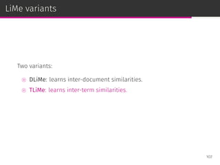
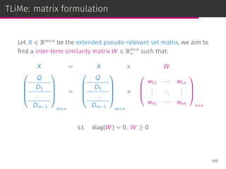
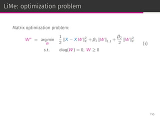
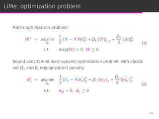
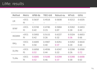
![LiMe: Linear Methods for PRF
Linear methods such as SLIM have been successfully used in
recommendation [Ning & Karypis, ICDM ’11].
We adapt them to PRF. Our proposal LiMe:
⊚ models the PRF task a matrix decomposition problem
⊚ employs linear methods to provide a solution
⊚ is able to learn inter-term or inter-doc similarities
⊚ jointly models the query and the pseudo-relevant set
⊚ admits different feature schemes
⊚ is agnostic to the retrieval model
106](https://image.slidesharecdn.com/slides-190509153630/85/Information-Retrieval-Models-for-Recommender-Systems-PhD-slides-167-320.jpg)


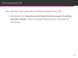


![Conferences (I)
gitemizeitemize4 [gitemize,1] leftmargin=0.3cm+, label=
A. Landin, D. Valcarce, J. Parapar, Á. Barreiro. “PRIN: A Probabilistic
Recommender with Item Priors and Neural Models”. ECIR ’19, pp.
133-147, 2019.
D. Valcarce, A. Bellogín, J. Parapar, P. Castells. “On the Robustness and
Discriminative Power of IR Metrics for Top-N Recommendation”.
ACM RecSys ’18, pp. 260-268, 2018.
D. Valcarce, J. Parapar, Á. Barreiro. “LiMe: Linear Methods for
Pseudo-Relevance Feedback”. ACM SAC ’18, pp. 678-687, 2018.
D. Valcarce, J. Parapar, Á. Barreiro. “Combining Top-N Recommenders
with Metasearch Algorithms”. ACM SIGIR ’17, pp. 805-808, 2017.
D. Valcarce, J. Parapar, Á. Barreiro. “Additive Smoothing for
Relevance-Based Language Modelling of Recommender Systems”. 121](https://image.slidesharecdn.com/slides-190509153630/85/Information-Retrieval-Models-for-Recommender-Systems-PhD-slides-193-320.jpg)
![Conferences (II)
gitemizeitemize4 [gitemize,1] leftmargin=0.3cm+, label=
D. Valcarce, J. Parapar, Á. Barreiro. “Efficient Pseudo-Relevance
Feedback Methods for Collaborative Filtering Recommendation”.
ECIR ’16, pp. 602-613, 2016.
D. Valcarce, J. Parapar, Á. Barreiro. “Language Models for Collaborative
Filtering Neighbourhoods”. ECIR ’16, pp. 614-625, 2016.
D. Valcarce. “Exploring Statistical Language Models for Recommender
Systems”. ACM RecSys ’15, pp. 375-378, 2015.
D. Valcarce, J. Parapar, Á. Barreiro. “A Study of Priors for
Relevance-Based Language Modelling of Recommender Systems”.
ACM RecSys ’15, pp. 237-240, 2015.
D. Valcarce, J. Parapar, Á. Barreiro. “A Study of Smoothing Methods for
Relevance-Based Language Modelling of Recommender Systems”. 122](https://image.slidesharecdn.com/slides-190509153630/85/Information-Retrieval-Models-for-Recommender-Systems-PhD-slides-194-320.jpg)
![Journals
gitemizeitemize4 [gitemize,1] leftmargin=0.3cm+, label=
D. Valcarce, J. Parapar, Á. Barreiro. “Document-based and Term-based Linear Methods
for Pseudo-Relevance Feedback”. Applied Computing Review 18(4), pp. 5-17, 2018.
D. Valcarce, I. Brilhante, J.A. Macedo, F.M. Nardini, R. Perego, C. Renso. “Item-driven
group formation”. Online Social Networks and Media 8, pp. 17-31, 2018.
D. Valcarce, J. Parapar, Á. Barreiro. “Finding and Analysing Good Neighbourhoods to
Improve Collaborative Filtering”. Knowledge-Based Systems 159, pp. 193-202, 2018.
D. Valcarce, J. Parapar, Á. Barreiro. “A MapReduce implementation of posterior
probability clustering and relevance models for recommendation”. Engineering
Applications of Artificial Intelligence 75, pp. 114-124, 2018.
D. Valcarce, J. Parapar, Á. Barreiro. “Axiomatic Analysis of Language Modelling of
Recommender Systems”. International Journal of Uncertainty, Fuzziness and
Knowledge-Based Systems 25(2), pp. 113-128, 2017.
D. Valcarce, J. Parapar, Á. Barreiro. “Item-Based Relevance Modelling of
Recommendations for Getting Rid of Long Tail Products”. Knowledge-Based Systems
103, pp. 41-51, 2016. 123](https://image.slidesharecdn.com/slides-190509153630/85/Information-Retrieval-Models-for-Recommender-Systems-PhD-slides-195-320.jpg)


![LiMe: Linear Methods for Pseudo-Relevance Feedback [SAC '18 Slides]](https://cdn.slidesharecdn.com/ss_thumbnails/limeslides-180411100357-thumbnail.jpg?width=640&height=640&fit=bounds)


![Language Models for Collaborative Filtering Neighbourhoods [ECIR '16 Slides]](https://cdn.slidesharecdn.com/ss_thumbnails/slides-2016-lmforneigh-160411083912-thumbnail.jpg?width=640&height=640&fit=bounds)


