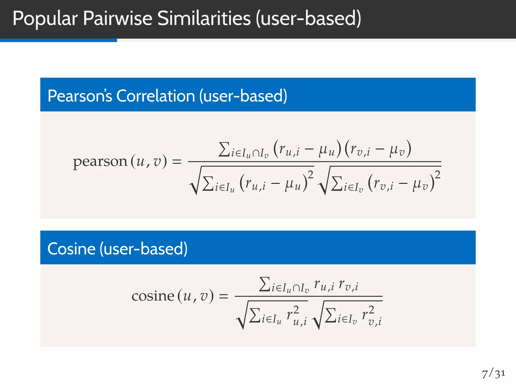
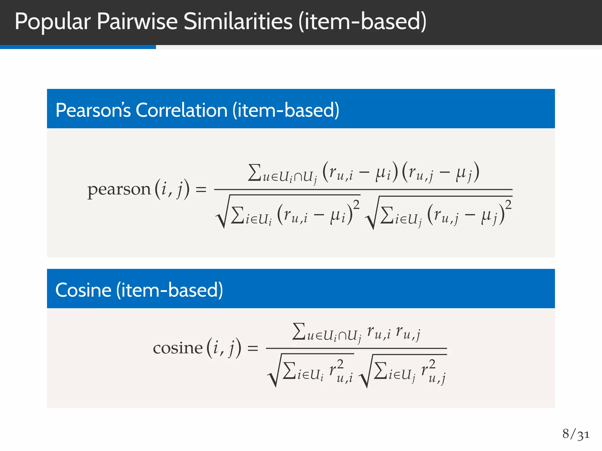
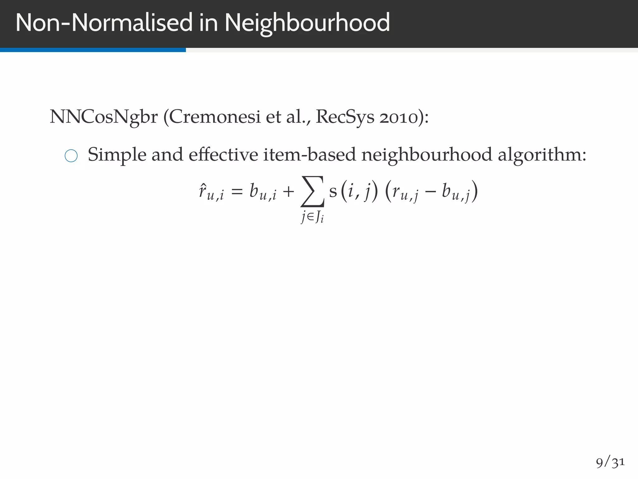
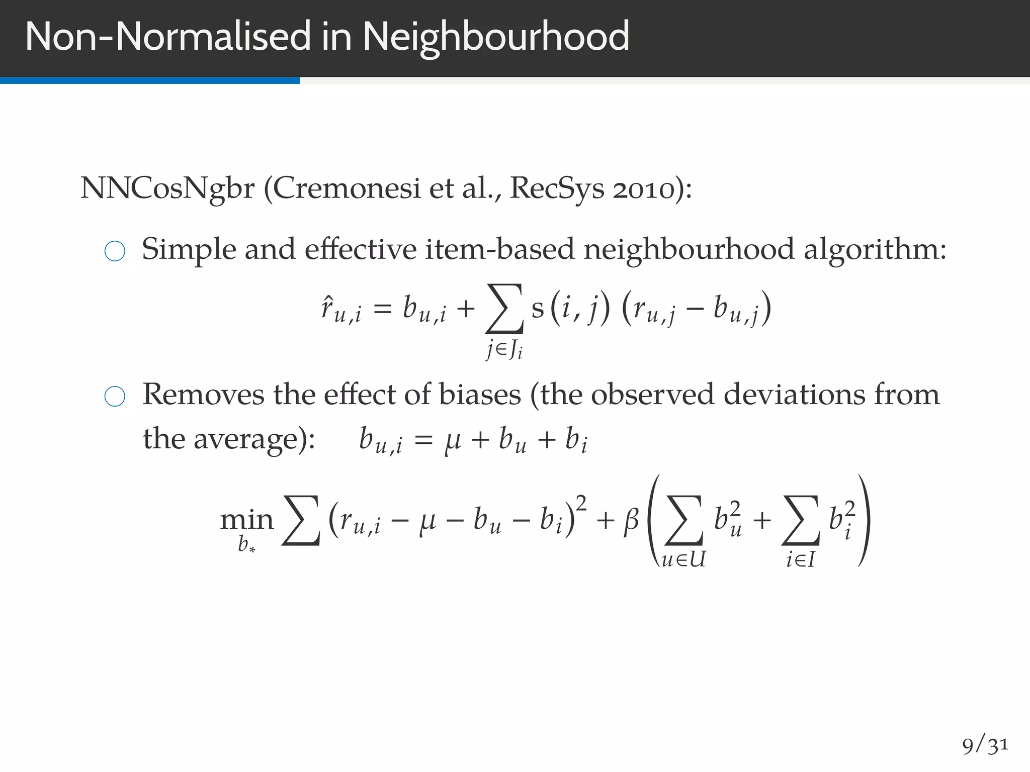
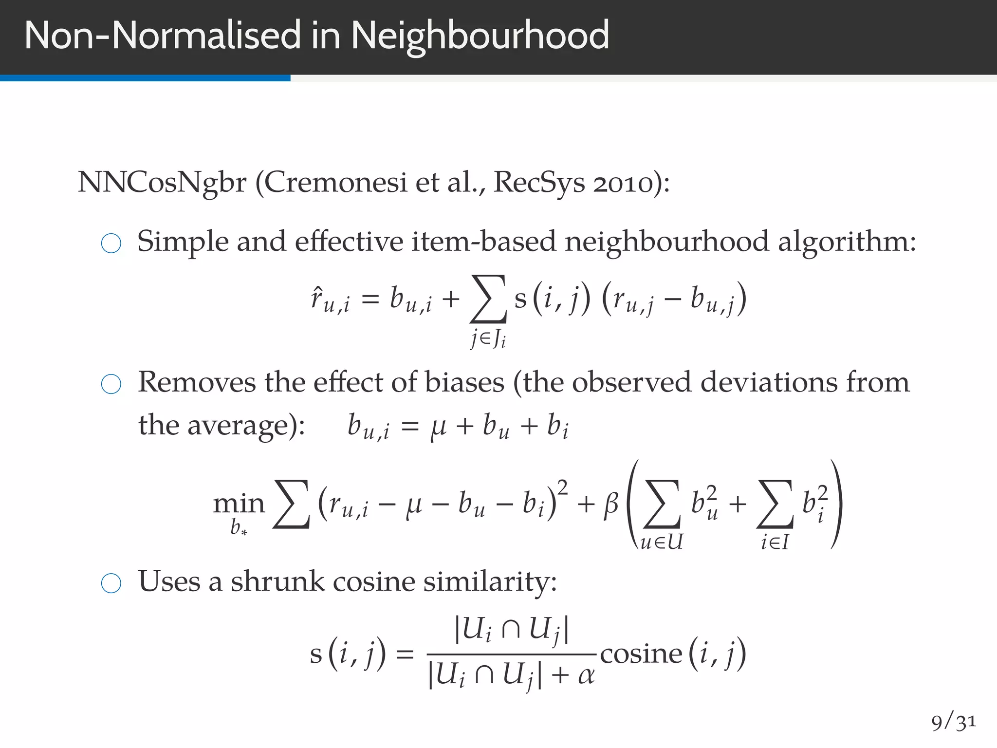
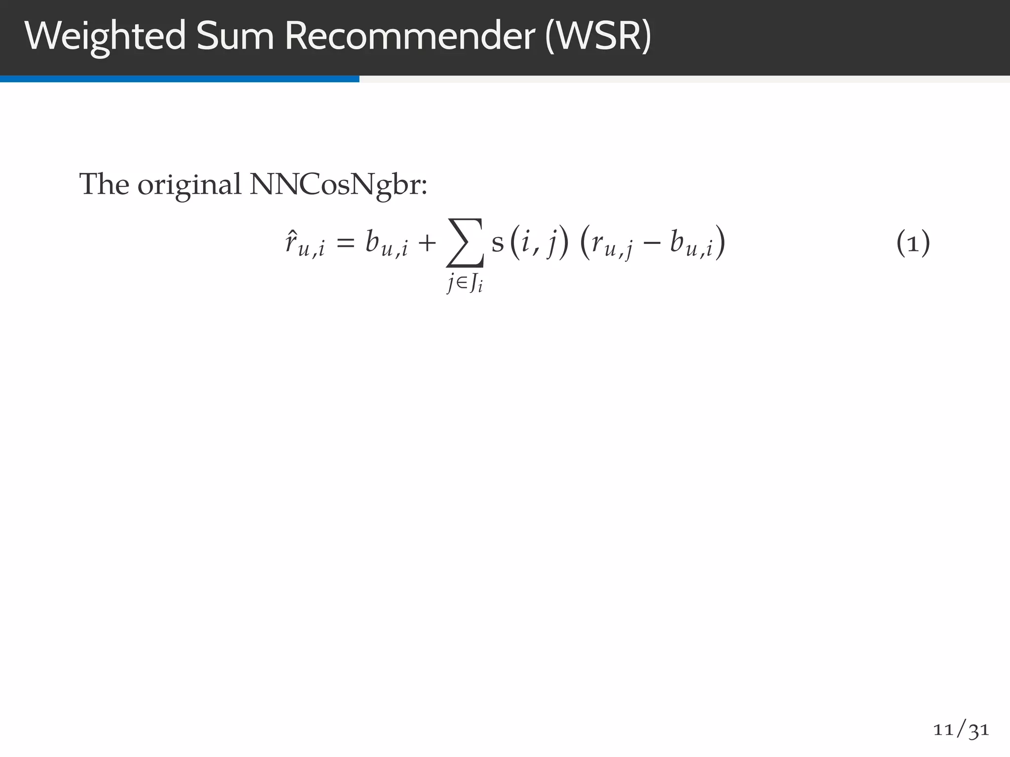
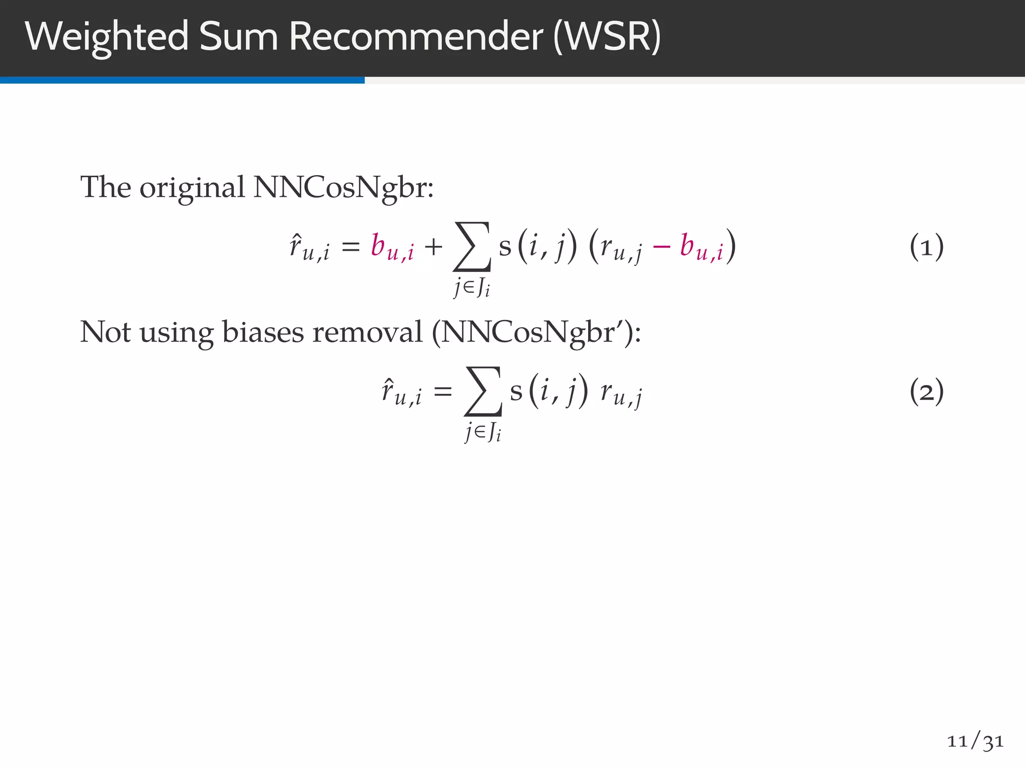
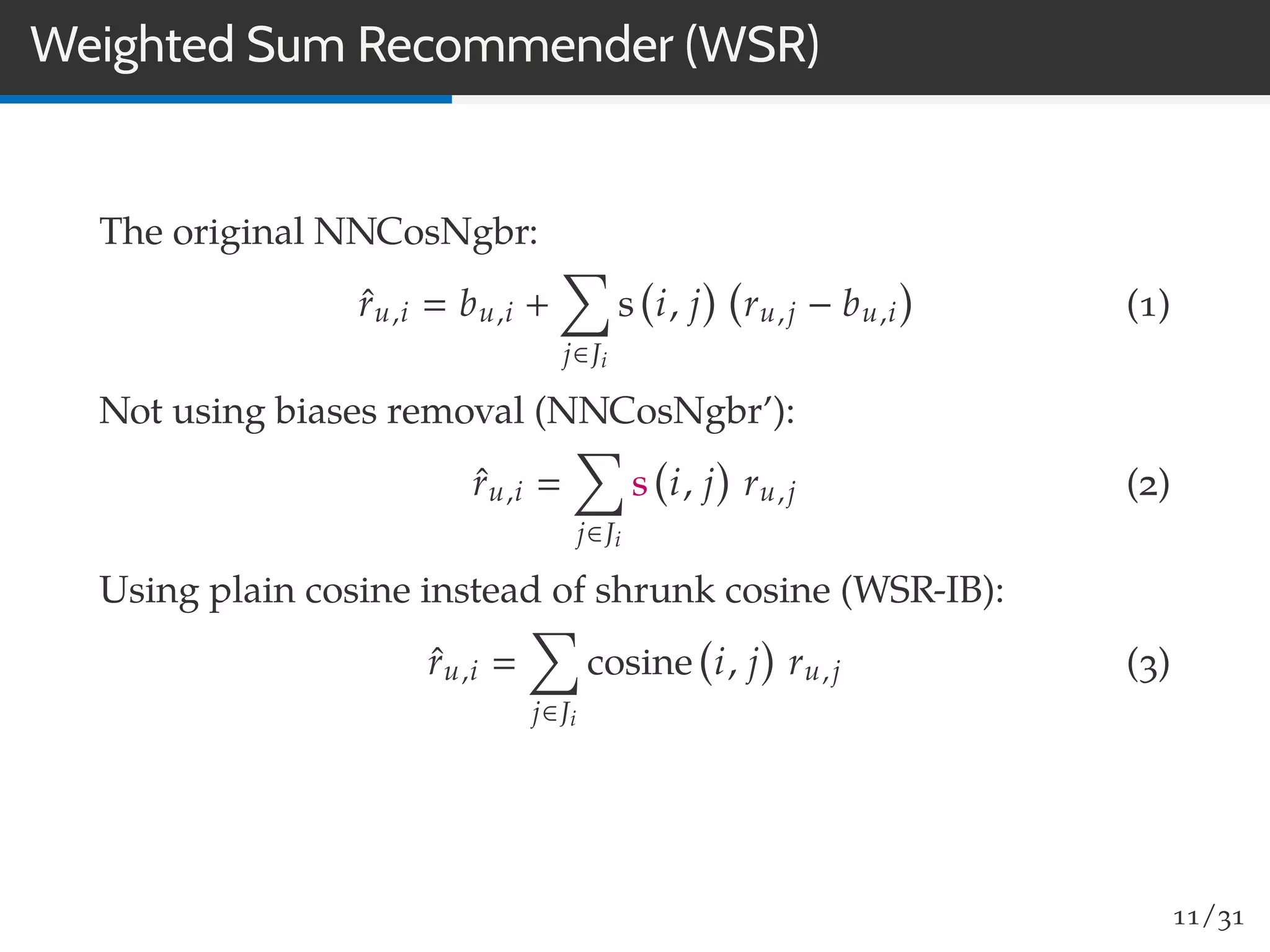
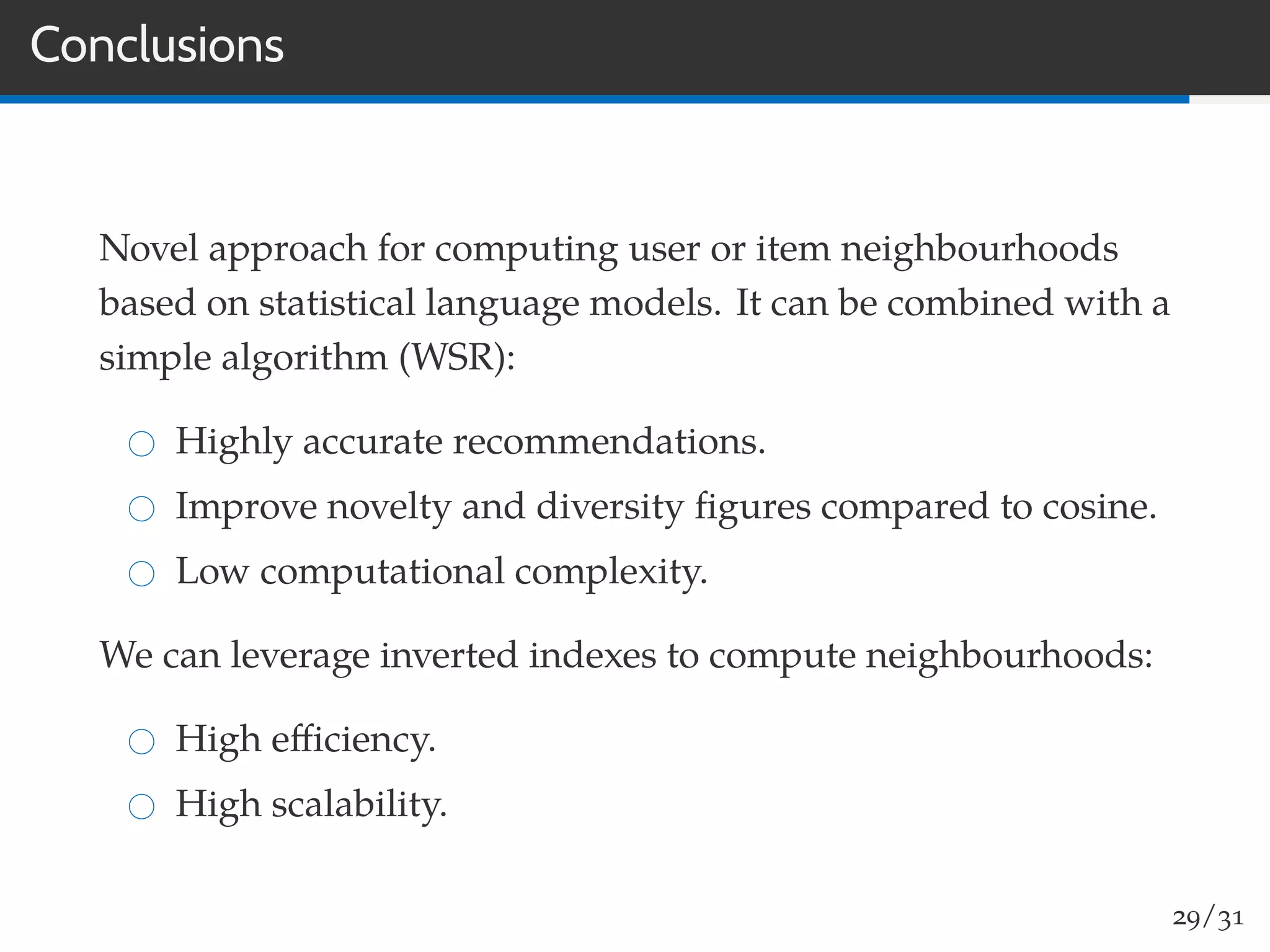
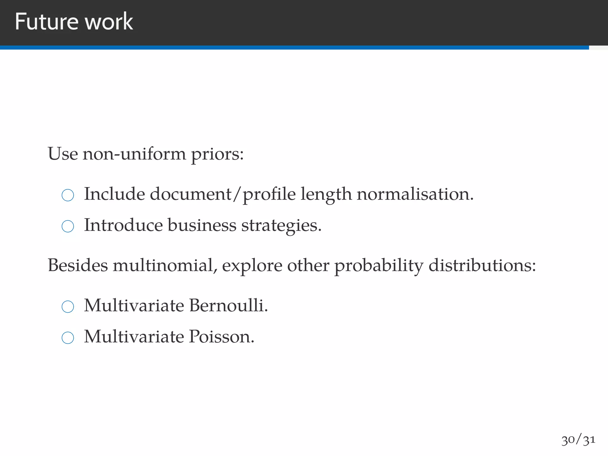
ECIR 2016, PADUA, ITALY
LANGUAGE MODELS FOR COLLABORATIVE FILTERING
NEIGHBOURHOODS
Daniel Valcarce, Javier Parapar, Álvaro Barreiro
@dvalcarce @jparapar @AlvaroBarreiroG
Information Retrieval Lab
@IRLab_UDC
University of A Coruña
Spain
Outline
1. Recommender Systems
2. Weighted Sum Recommender (WSR)
3. Improving WSR
4. Language Models for Neighbourhoods
5. Experiments
6. Conclusions and Future Directions
1/31
RECOMMENDER SYSTEMS
Recommender Systems
Recommender systems aim to provide items that may be of
interest to the users.
Top-N recommendation techniques create a ranking of the N
most relevant items for each user.
Main categories:
Content-based: exploits item metadata to recommend
items similar to those the target user liked in the past.
Collaborative filtering: relies on the user feedback such as
ratings or clicks.
Hybrid: combination of content-based and collaborative
filtering approaches.
3/31
Collaborative Filtering
Collaborative Filtering (CF) exploit feedback from users:
Explicit: ratings or reviews.
Implicit: clicks or purchases.
Two main families of CF methods:
Model-based: learn a model from the data and use it for
recommendation.
Neighbourhood-based (or memory-based): compute
recommendations using directly part of the ratings.
4/31
Notation
The set of users U
The set of items I
The rating that the user u gave to the item i is ru,i
The set of items rated by user u is denoted by Iu
The set of users that rated item i is denoted by Ui
The average rating of user u is denoted by µu
The average rating of item i is denoted by µi
The user neighbourhood of user u is denoted by Vu
The item neighbourhood of item i is denoted by Ji
5/31
Neighbourhood-based Methods
Two perspectives:
User-based: recommend items that users with common
interests with you liked.
Item-based: recommend items similar to those you liked.
Similarity between items is computed using common users
among items (not the content!).
The effectiveness of neighbourhood-based methods relies
largely on how neighbours are computed.
The most common approach is to compute the k nearest
neighbours (k-NN algorithm) using a pairwise similarity.
6/31
Popular Pairwise Similarities (user-based)
Pearson’s Correlation (user-based)
pearson (u, v)
i∈Iu∩Iv
ru,i − µu rv,i − µv
i∈Iu
ru,i − µu
2
i∈Iv
rv,i − µv
2
Cosine (user-based)
cosine (u, v)
i∈Iu∩Iv
ru,i rv,i
i∈Iu
r2
u,i i∈Iv
r2
v,i
7/31
Popular Pairwise Similarities (item-based)
Pearson’s Correlation (item-based)
pearson i, j
u∈Ui∩Uj
ru,i − µi ru,j − µj
i∈Ui
ru,i − µi
2
i∈Uj
ru,j − µj
2
Cosine (item-based)
cosine i, j
u∈Ui∩Uj
ru,i ru,j
i∈Ui
r2
u,i i∈Uj
r2
u,j
8/31
Non-Normalised in Neighbourhood
NNCosNgbr (Cremonesi et al., RecSys 2010):
Simple and effective item-based neighbourhood algorithm:
ˆru,i bu,i +
j∈Ji
s i, j ru,j − bu,j
9/31
Non-Normalised in Neighbourhood
NNCosNgbr (Cremonesi et al., RecSys 2010):
Simple and effective item-based neighbourhood algorithm:
ˆru,i bu,i +
j∈Ji
s i, j ru,j − bu,j
Removes the effect of biases (the observed deviations from
the average): bu,i µ + bu + bi
min
b∗
ru,i − µ − bu − bi
2
+ β
u∈U
b2
u +
i∈I
b2
i
Uses a shrunk cosine similarity:
s i, j
|Ui ∩ Uj|
|Ui ∩ Uj| + α
cosine i, j
9/31
WEIGHTED SUM RECOMMENDER (WSR)
Weighted Sum Recommender (WSR)
The original NNCosNgbr:
ˆru,i bu,i +
j∈Ji
s i, j ru,j − bu,i (1)
11/31
Weighted Sum Recommender (WSR)
The original NNCosNgbr:
ˆru,i bu,i +
j∈Ji
s i, j ru,j − bu,i (1)
Not using biases removal (NNCosNgbr’):
ˆru,i
j∈Ji
s i, j ru,j (2)
11/31
Weighted Sum Recommender (WSR)
The original NNCosNgbr:
ˆru,i bu,i +
j∈Ji
s i, j ru,j − bu,i (1)
Not using biases removal (NNCosNgbr’):
ˆru,i
j∈Ji
s i, j ru,j (2)
Using plain cosine instead of shrunk cosine (WSR-IB):
ˆru,i
j∈Ji
cosine i, j ru,j (3)
11/31
Weighted Sum Recommender (WSR)
The original NNCosNgbr:
ˆru,i bu,i +
j∈Ji
s i, j ru,j − bu,i (1)
Not using biases removal (NNCosNgbr’):
ˆru,i
j∈Ji
s i, j ru,j (2)
Using plain cosine instead of shrunk cosine (WSR-IB):
ˆru,i
j∈Ji
cosine i, j ru,j (3)
Also the user-based version (WSR-UB):
ˆru,i
v∈Vu
cosine (u, v) rv,i (4)
11/31
Experiments with WSR
Algorithm ML 100k ML 1M R3-Yahoo! LibraryThing
NNCosNgr 0.1427 0.1042 0.0138 0.0550
NNCosNgr’ 0.3704a 0.3334a 0.0257a 0.2217ad
WSR-IB 0.3867ab 0.3382ab 0.0274ab 0.2539abd
WSR-UB 0.3899ab 0.3430ab 0.0261a 0.1906a
Table: Values of nDCG@10. Statistical significance is superscripted
(Wilcoxon two-sided p < 0.01). Pink = best algorithm. Blue = not
significantly different to the best.
12/31
IMPROVING WSR
Improving WSR
Can we do better with this simple approach (WSR)?
14/31
Improving WSR
Can we do better with this simple approach (WSR)? Yes!
Pairwise similarities have a huge impact on performance.
Cosine provides important improvements over Pearson’s
correlation coefficient (Cremonesi et al., RecSys 2010).
Let’s study cosine similarity from the perspective of
Information Retrieval.
14/31
Cosine Similarity and the Vector Space Model
Recommendation Information Retrieval
Target user Query
Rest of users Documents
Items Terms
15/31
Cosine Similarity and the Vector Space Model
Recommendation Information Retrieval
Target user Query
Rest of users Documents
Items Terms
Under this scheme, using cosine similarity for finding
neighbours is equivalent to search in the Vector Space Model.
15/31
Cosine Similarity and the Vector Space Model
Recommendation Information Retrieval
Target user Query
Rest of users Documents
Items Terms
Under this scheme, using cosine similarity for finding
neighbours is equivalent to search in the Vector Space Model.
If we swap users and items, we can derive an analogous
item-based approach.
We can use sophisticated search techniques for finding
neighbours!
15/31
LANGUAGE MODELS FOR NEIGHBOURHOODS
Language Models
Statistical language models are a state-of-the-art framework for
document retrieval.
Documents are ranked according to their posterior probability
given the query:
p(d|q)
p(q|d) p(d)
p(q)
rank
p(q|d) p(d)
17/31
Language Models
Statistical language models are a state-of-the-art framework for
document retrieval.
Documents are ranked according to their posterior probability
given the query:
p(d|q)
p(q|d) p(d)
p(q)
rank
p(q|d) p(d)
The query likelihood, p(q|d), is based on a unigram model:
p(q|d)
t∈q
p(t|d)c(t,d)
The document prior, p(d), is usually considered uniform.
17/31
Language Models for Finding Neighbourhoods (I)
Information Retrieval:
p(d|q)
rank
p(d)
t∈q
p(t|d)c(t,d)
User-based collaborative filtering:
p(v|u)
rank
p(v)
i∈Iu
p(i|v)rv,i
Item-based collaborative filtering:
p(j|i)
rank
p(j)
u∈Ui
p(u|j)ru,j
18/31
Language Models for Finding Neighbourhoods (II)
User-based collaborative filtering:
p(v|u)
rank
p(v)
i∈Iu
p(i|v)rv,i
We assume a multinomial distribution over the count of ratings.
The maximum likelihood estimate (MLE) is:
pmle(i|v)
rv,i
j∈Iv
rv,j
19/31
Language Models for Finding Neighbourhoods (II)
User-based collaborative filtering:
p(v|u)
rank
p(v)
i∈Iu
p(i|v)rv,i
We assume a multinomial distribution over the count of ratings.
The maximum likelihood estimate (MLE) is:
pmle(i|v)
rv,i
j∈Iv
rv,j
However it suffers from sparsity. We need smoothing!
19/31
Smoothing Methods for Language Models
Absolute Discounting (AD)
pδ(i|u)
max(ru,i − δ, 0) + δ |Iu| p(i|C)
j∈Iu
ru,j
Jelinek-Mercer (JM)
pλ(i|u) (1 − λ)
ru,i
j∈Iu
ru,j
+ λ p(i|C)
Dirichlet Priors (DP)
pµ(i|u)
ru,i + µ p(i|C)
µ + j∈Iu
ru,j
20/31
EXPERIMENTS
Experimental settings
Baselines:
Pearson’s correlation coefficient
RM1Sim: user-based similarity (Bellogín et al., RecSys’13)
Cosine similarity
Our similarities are Language Models using:
Absolute Discounting smoothing
Jelinek-Mercer smoothing
Dirichlet Priors smoothing
22/31
Parameter Sensibility of WSR-UB on MovieLens 100k
0.18
0 1k 2k 3k 4k 5k 6k 7k 8k 9k 10k
0.28
0.30
0.32
0.34
0.36
0.38
0.40
0 0.1 0.2 0.3 0.4 0.5 0.6 0.7 0.8 0.9 1
µ
nDCG@10
λ, δ
Pearson
Cosine
RM1Sim (λ)
LM-Absolute Discounting (δ)
LM-Jelinek-Mercer (λ)
LM-Dirichlet Priors (µ)
23/31
Parameter Sensibility of WSR-IB on R3-Yahoo!
0.012
0.014
0.016
0.018
0.020
0.022
0.024
0.026
0.028
0.030
100
101
102
103
104
105
106
0 0.1 0.2 0.3 0.4 0.5 0.6 0.7 0.8 0.9 1
nDCG@10
µ
λ, δ
Pearson
Cosine
LM-Absolute Discounting (δ)
LM-Jelinek-Mercer (λ)
LM-Dirichlet Priors (µ)
24/31
Precision (nDCG@10)
Algorithm ML 100k ML 1M R3-Yahoo LibraryThing
NNCosNgbr 0.1427 0.1042 0.0138 0.0550
PureSVD 0.3595a 0.3499ac 0.0198a 0.2245a
Cosine-WSR 0.3899ab 0.3430a 0.0274ab 0.2476ab
LM-DP-WSR 0.4017abc 0.3585abc 0.0271ab 0.2464ab
LM-JM-WSR 0.4013abc 0.3622abcd 0.0276ab 0.2537abcd
Table: Values of precision in terms of normalised discounted
cumulative gain at 10. Statistical significance is superscripted
(Wilcoxon two-sided p < 0.01). Pink = best algorithm. Blue = not
significantly different to the best.
25/31
Diversity (Gini@10)
Algorithm ML 100k ML 1M R3-Yahoo! LibraryThing
Cosine-WSR 0.0549 0.0400 0.0902 0.1025
LM-DP-WSR 0.0659 0.0435 0.1557 0.1356
LM-JM-WSR 0.0627 0.0435 0.1034 0.1245
Table: Values of the complement of the Gini index at 10.
Pink = best algorithm.
26/31
Novelty (MSI@10)
Algorithm ML 100k ML 1M R3-Yahoo! LibraryThing
Cosine-WSR 11.0579 12.4816 21.1968 41.1462
LM-DP-WSR 11.5219 12.8040 25.9647 46.4197
LM-JM-WSR 11.3921 12.8417 21.7935 43.5986
Table: Values of novelty in terms of Mean Self Information at 10.
Pink = best algorithm.
27/31
CONCLUSIONS AND FUTURE DIRECTIONS
Conclusions
Novel approach for computing user or item neighbourhoods
based on statistical language models. It can be combined with a
simple algorithm (WSR):
Highly accurate recommendations.
Improve novelty and diversity figures compared to cosine.
Low computational complexity.
We can leverage inverted indexes to compute neighbourhoods:
High efficiency.
High scalability.
29/31
Future work
Use non-uniform priors:
Include document/profile length normalisation.
Introduce business strategies.
Besides multinomial, explore other probability distributions:
Multivariate Bernoulli.
Multivariate Poisson.
30/31
THANK YOU!
@DVALCARCE
http://www.dc.fi.udc.es/~dvalcarce

Language Models for Collaborative Filtering Neighbourhoods [ECIR '16 Slides]

  • 1.
    ECIR 2016, PADUA,ITALY LANGUAGE MODELS FOR COLLABORATIVE FILTERING NEIGHBOURHOODS Daniel Valcarce, Javier Parapar, Álvaro Barreiro @dvalcarce @jparapar @AlvaroBarreiroG Information Retrieval Lab @IRLab_UDC University of A Coruña Spain
  • 2.
    Outline 1. Recommender Systems 2.Weighted Sum Recommender (WSR) 3. Improving WSR 4. Language Models for Neighbourhoods 5. Experiments 6. Conclusions and Future Directions 1/31
  • 3.
  • 4.
    Recommender Systems Recommender systemsaim to provide items that may be of interest to the users. Top-N recommendation techniques create a ranking of the N most relevant items for each user. Main categories: Content-based: exploits item metadata to recommend items similar to those the target user liked in the past. Collaborative filtering: relies on the user feedback such as ratings or clicks. Hybrid: combination of content-based and collaborative filtering approaches. 3/31
  • 5.
    Recommender Systems Recommender systemsaim to provide items that may be of interest to the users. Top-N recommendation techniques create a ranking of the N most relevant items for each user. Main categories: Content-based: exploits item metadata to recommend items similar to those the target user liked in the past. Collaborative filtering: relies on the user feedback such as ratings or clicks. Hybrid: combination of content-based and collaborative filtering approaches. 3/31
  • 6.
    Collaborative Filtering Collaborative Filtering(CF) exploit feedback from users: Explicit: ratings or reviews. Implicit: clicks or purchases. Two main families of CF methods: Model-based: learn a model from the data and use it for recommendation. Neighbourhood-based (or memory-based): compute recommendations using directly part of the ratings. 4/31
  • 7.
    Collaborative Filtering Collaborative Filtering(CF) exploit feedback from users: Explicit: ratings or reviews. Implicit: clicks or purchases. Two main families of CF methods: Model-based: learn a model from the data and use it for recommendation. Neighbourhood-based (or memory-based): compute recommendations using directly part of the ratings. 4/31
  • 8.
    Notation The set ofusers U The set of items I The rating that the user u gave to the item i is ru,i The set of items rated by user u is denoted by Iu The set of users that rated item i is denoted by Ui The average rating of user u is denoted by µu The average rating of item i is denoted by µi The user neighbourhood of user u is denoted by Vu The item neighbourhood of item i is denoted by Ji 5/31
  • 9.
    Neighbourhood-based Methods Two perspectives: User-based:recommend items that users with common interests with you liked. Item-based: recommend items similar to those you liked. Similarity between items is computed using common users among items (not the content!). The effectiveness of neighbourhood-based methods relies largely on how neighbours are computed. The most common approach is to compute the k nearest neighbours (k-NN algorithm) using a pairwise similarity. 6/31
  • 10.
    Popular Pairwise Similarities(user-based) Pearson’s Correlation (user-based) pearson (u, v) i∈Iu∩Iv ru,i − µu rv,i − µv i∈Iu ru,i − µu 2 i∈Iv rv,i − µv 2 Cosine (user-based) cosine (u, v) i∈Iu∩Iv ru,i rv,i i∈Iu r2 u,i i∈Iv r2 v,i 7/31
  • 11.
    Popular Pairwise Similarities(item-based) Pearson’s Correlation (item-based) pearson i, j u∈Ui∩Uj ru,i − µi ru,j − µj i∈Ui ru,i − µi 2 i∈Uj ru,j − µj 2 Cosine (item-based) cosine i, j u∈Ui∩Uj ru,i ru,j i∈Ui r2 u,i i∈Uj r2 u,j 8/31
  • 12.
    Non-Normalised in Neighbourhood NNCosNgbr(Cremonesi et al., RecSys 2010): Simple and effective item-based neighbourhood algorithm: ˆru,i bu,i + j∈Ji s i, j ru,j − bu,j 9/31
  • 13.
    Non-Normalised in Neighbourhood NNCosNgbr(Cremonesi et al., RecSys 2010): Simple and effective item-based neighbourhood algorithm: ˆru,i bu,i + j∈Ji s i, j ru,j − bu,j Removes the effect of biases (the observed deviations from the average): bu,i µ + bu + bi min b∗ ru,i − µ − bu − bi 2 + β u∈U b2 u + i∈I b2 i 9/31
  • 14.
    Non-Normalised in Neighbourhood NNCosNgbr(Cremonesi et al., RecSys 2010): Simple and effective item-based neighbourhood algorithm: ˆru,i bu,i + j∈Ji s i, j ru,j − bu,j Removes the effect of biases (the observed deviations from the average): bu,i µ + bu + bi min b∗ ru,i − µ − bu − bi 2 + β u∈U b2 u + i∈I b2 i Uses a shrunk cosine similarity: s i, j |Ui ∩ Uj| |Ui ∩ Uj| + α cosine i, j 9/31
  • 15.
  • 16.
    Weighted Sum Recommender(WSR) The original NNCosNgbr: ˆru,i bu,i + j∈Ji s i, j ru,j − bu,i (1) 11/31
  • 17.
    Weighted Sum Recommender(WSR) The original NNCosNgbr: ˆru,i bu,i + j∈Ji s i, j ru,j − bu,i (1) Not using biases removal (NNCosNgbr’): ˆru,i j∈Ji s i, j ru,j (2) 11/31
  • 18.
    Weighted Sum Recommender(WSR) The original NNCosNgbr: ˆru,i bu,i + j∈Ji s i, j ru,j − bu,i (1) Not using biases removal (NNCosNgbr’): ˆru,i j∈Ji s i, j ru,j (2) Using plain cosine instead of shrunk cosine (WSR-IB): ˆru,i j∈Ji cosine i, j ru,j (3) 11/31
  • 19.
    Weighted Sum Recommender(WSR) The original NNCosNgbr: ˆru,i bu,i + j∈Ji s i, j ru,j − bu,i (1) Not using biases removal (NNCosNgbr’): ˆru,i j∈Ji s i, j ru,j (2) Using plain cosine instead of shrunk cosine (WSR-IB): ˆru,i j∈Ji cosine i, j ru,j (3) Also the user-based version (WSR-UB): ˆru,i v∈Vu cosine (u, v) rv,i (4) 11/31
  • 20.
    Experiments with WSR AlgorithmML 100k ML 1M R3-Yahoo! LibraryThing NNCosNgr 0.1427 0.1042 0.0138 0.0550 NNCosNgr’ 0.3704a 0.3334a 0.0257a 0.2217ad WSR-IB 0.3867ab 0.3382ab 0.0274ab 0.2539abd WSR-UB 0.3899ab 0.3430ab 0.0261a 0.1906a Table: Values of nDCG@10. Statistical significance is superscripted (Wilcoxon two-sided p < 0.01). Pink = best algorithm. Blue = not significantly different to the best. 12/31
  • 21.
  • 22.
    Improving WSR Can wedo better with this simple approach (WSR)? 14/31
  • 23.
    Improving WSR Can wedo better with this simple approach (WSR)? Yes! Pairwise similarities have a huge impact on performance. Cosine provides important improvements over Pearson’s correlation coefficient (Cremonesi et al., RecSys 2010). Let’s study cosine similarity from the perspective of Information Retrieval. 14/31
  • 24.
    Cosine Similarity andthe Vector Space Model Recommendation Information Retrieval Target user Query Rest of users Documents Items Terms 15/31
  • 25.
    Cosine Similarity andthe Vector Space Model Recommendation Information Retrieval Target user Query Rest of users Documents Items Terms Under this scheme, using cosine similarity for finding neighbours is equivalent to search in the Vector Space Model. 15/31
  • 26.
    Cosine Similarity andthe Vector Space Model Recommendation Information Retrieval Target user Query Rest of users Documents Items Terms Under this scheme, using cosine similarity for finding neighbours is equivalent to search in the Vector Space Model. If we swap users and items, we can derive an analogous item-based approach. 15/31
  • 27.
    Cosine Similarity andthe Vector Space Model Recommendation Information Retrieval Target user Query Rest of users Documents Items Terms Under this scheme, using cosine similarity for finding neighbours is equivalent to search in the Vector Space Model. If we swap users and items, we can derive an analogous item-based approach. We can use sophisticated search techniques for finding neighbours! 15/31
  • 28.
    LANGUAGE MODELS FORNEIGHBOURHOODS
  • 29.
    Language Models Statistical languagemodels are a state-of-the-art framework for document retrieval. Documents are ranked according to their posterior probability given the query: p(d|q) p(q|d) p(d) p(q) rank p(q|d) p(d) 17/31
  • 30.
    Language Models Statistical languagemodels are a state-of-the-art framework for document retrieval. Documents are ranked according to their posterior probability given the query: p(d|q) p(q|d) p(d) p(q) rank p(q|d) p(d) The query likelihood, p(q|d), is based on a unigram model: p(q|d) t∈q p(t|d)c(t,d) 17/31
  • 31.
    Language Models Statistical languagemodels are a state-of-the-art framework for document retrieval. Documents are ranked according to their posterior probability given the query: p(d|q) p(q|d) p(d) p(q) rank p(q|d) p(d) The query likelihood, p(q|d), is based on a unigram model: p(q|d) t∈q p(t|d)c(t,d) The document prior, p(d), is usually considered uniform. 17/31
  • 32.
    Language Models forFinding Neighbourhoods (I) Information Retrieval: p(d|q) rank p(d) t∈q p(t|d)c(t,d) User-based collaborative filtering: p(v|u) rank p(v) i∈Iu p(i|v)rv,i Item-based collaborative filtering: p(j|i) rank p(j) u∈Ui p(u|j)ru,j 18/31
  • 33.
    Language Models forFinding Neighbourhoods (II) User-based collaborative filtering: p(v|u) rank p(v) i∈Iu p(i|v)rv,i We assume a multinomial distribution over the count of ratings. The maximum likelihood estimate (MLE) is: pmle(i|v) rv,i j∈Iv rv,j 19/31
  • 34.
    Language Models forFinding Neighbourhoods (II) User-based collaborative filtering: p(v|u) rank p(v) i∈Iu p(i|v)rv,i We assume a multinomial distribution over the count of ratings. The maximum likelihood estimate (MLE) is: pmle(i|v) rv,i j∈Iv rv,j However it suffers from sparsity. We need smoothing! 19/31
  • 35.
    Smoothing Methods forLanguage Models Absolute Discounting (AD) pδ(i|u) max(ru,i − δ, 0) + δ |Iu| p(i|C) j∈Iu ru,j Jelinek-Mercer (JM) pλ(i|u) (1 − λ) ru,i j∈Iu ru,j + λ p(i|C) Dirichlet Priors (DP) pµ(i|u) ru,i + µ p(i|C) µ + j∈Iu ru,j 20/31
  • 36.
  • 37.
    Experimental settings Baselines: Pearson’s correlationcoefficient RM1Sim: user-based similarity (Bellogín et al., RecSys’13) Cosine similarity Our similarities are Language Models using: Absolute Discounting smoothing Jelinek-Mercer smoothing Dirichlet Priors smoothing 22/31
  • 38.
    Parameter Sensibility ofWSR-UB on MovieLens 100k 0.18 0 1k 2k 3k 4k 5k 6k 7k 8k 9k 10k 0.28 0.30 0.32 0.34 0.36 0.38 0.40 0 0.1 0.2 0.3 0.4 0.5 0.6 0.7 0.8 0.9 1 µ nDCG@10 λ, δ Pearson Cosine RM1Sim (λ) LM-Absolute Discounting (δ) LM-Jelinek-Mercer (λ) LM-Dirichlet Priors (µ) 23/31
  • 39.
    Parameter Sensibility ofWSR-IB on R3-Yahoo! 0.012 0.014 0.016 0.018 0.020 0.022 0.024 0.026 0.028 0.030 100 101 102 103 104 105 106 0 0.1 0.2 0.3 0.4 0.5 0.6 0.7 0.8 0.9 1 nDCG@10 µ λ, δ Pearson Cosine LM-Absolute Discounting (δ) LM-Jelinek-Mercer (λ) LM-Dirichlet Priors (µ) 24/31
  • 40.
    Precision (nDCG@10) Algorithm ML100k ML 1M R3-Yahoo LibraryThing NNCosNgbr 0.1427 0.1042 0.0138 0.0550 PureSVD 0.3595a 0.3499ac 0.0198a 0.2245a Cosine-WSR 0.3899ab 0.3430a 0.0274ab 0.2476ab LM-DP-WSR 0.4017abc 0.3585abc 0.0271ab 0.2464ab LM-JM-WSR 0.4013abc 0.3622abcd 0.0276ab 0.2537abcd Table: Values of precision in terms of normalised discounted cumulative gain at 10. Statistical significance is superscripted (Wilcoxon two-sided p < 0.01). Pink = best algorithm. Blue = not significantly different to the best. 25/31
  • 41.
    Diversity (Gini@10) Algorithm ML100k ML 1M R3-Yahoo! LibraryThing Cosine-WSR 0.0549 0.0400 0.0902 0.1025 LM-DP-WSR 0.0659 0.0435 0.1557 0.1356 LM-JM-WSR 0.0627 0.0435 0.1034 0.1245 Table: Values of the complement of the Gini index at 10. Pink = best algorithm. 26/31
  • 42.
    Novelty (MSI@10) Algorithm ML100k ML 1M R3-Yahoo! LibraryThing Cosine-WSR 11.0579 12.4816 21.1968 41.1462 LM-DP-WSR 11.5219 12.8040 25.9647 46.4197 LM-JM-WSR 11.3921 12.8417 21.7935 43.5986 Table: Values of novelty in terms of Mean Self Information at 10. Pink = best algorithm. 27/31
  • 43.
  • 44.
    Conclusions Novel approach forcomputing user or item neighbourhoods based on statistical language models. It can be combined with a simple algorithm (WSR): Highly accurate recommendations. Improve novelty and diversity figures compared to cosine. Low computational complexity. We can leverage inverted indexes to compute neighbourhoods: High efficiency. High scalability. 29/31
  • 45.
    Future work Use non-uniformpriors: Include document/profile length normalisation. Introduce business strategies. Besides multinomial, explore other probability distributions: Multivariate Bernoulli. Multivariate Poisson. 30/31
  • 46.