a branch of statistics that uses sample data to make predictions, test hypotheses, and draw conclusions about a larger population, going beyond simple data description to generalize findings and measure uncertainty
Statistical Inference
• Astatistical hypothesis is a conjecture (an opinion or
conclusion formed on the basis of incomplete
information) concerning one or more populations.
3.
• The truthor falsity of a statistical hypothesis is never known
with absolute certainty unless we examine the entire
population
• we take a random sample from the population of interest and
use the data contained in this sample to provide evidence that
either supports or does not support the hypothesis
• Evidence from the sample that is inconsistent with the stated
hypothesis leads to a rejection of the hypothesis.
4.
The Role ofProbability in Hypothesis Testing
• suppose that the hypothesis postulated by the engineer is
that the fraction defective p in a certain process is 0.10.
• Suppose that 100 items are tested and 12 items are found
defective.
• It is reasonable to conclude that this evidence does not refute
the condition that the binomial parameter p = 0.10
• However, it also does not refute the chance that actually
p=0.12 or even higher
5.
The Role ofProbability in Hypothesis Testing
• But if we find 20 items defective, then we will get high
confidence and refute the hypothesis.
• firm conclusion is established by the data analyst when a
hypothesis is rejected.
• If the scientist is interested in strongly supporting a
contention, he or she hopes to arrive at the contention in the
form of rejection of a hypothesis.
• For example, If the medical researcher wishes to show strong
evidence in favor of the contention that coffee drinking
increases the risk of cancer, the hypothesis tested should be
of the form “there is no increase in cancer risk produced by
drinking coffee.”
6.
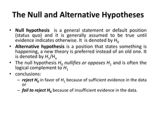
The Null andAlternative Hypotheses
• Null hypothesis is a general statement or default position
(status quo) and it is generally assumed to be true until
evidence indicates otherwise. It is denoted by H0
• Alternative hypothesis is a position that states something is
happening, a new theory is preferred instead of an old one. It
is denoted by H1/Ha
• The null hypothesis H0 nullifies or opposes H1 and is often the
logical complement to H1
• conclusions:
– reject H0 in favor of H1 because of sufficient evidence in the data
or
– fail to reject H0 because of insufficient evidence in the data.
7.
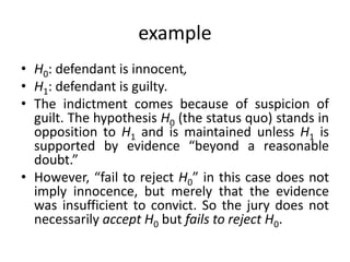
example
• H0: defendantis innocent,
• H1: defendant is guilty.
• The indictment comes because of suspicion of
guilt. The hypothesis H0 (the status quo) stands in
opposition to H1 and is maintained unless H1 is
supported by evidence “beyond a reasonable
doubt.”
• However, “fail to reject H0” in this case does not
imply innocence, but merely that the evidence
was insufficient to convict. So the jury does not
necessarily accept H0 but fails to reject H0.
8.
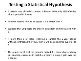
Testing a StatisticalHypothesis
• A certain type of cold vaccine (A) is known to be only 25% effective
after a period of 2 years.
• Another vaccine (B) is to be tested if it is better than A
• Suppose that 20 people are chosen at random and inoculated with
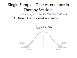
B
• If more than 8 of those receiving B surpass the 2-year period
without contracting the virus, then B will be considered superior to
A
• The requirement that the number exceed 8 is somewhat arbitrary
but appears reasonable in that it represents a modest gain over the
5 people
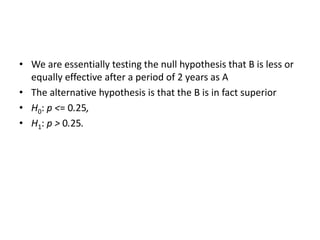
9.
• We areessentially testing the null hypothesis that B is less or
equally effective after a period of 2 years as A
• The alternative hypothesis is that the B is in fact superior
• H0: p <= 0.25,
• H1: p > 0.25.
10.
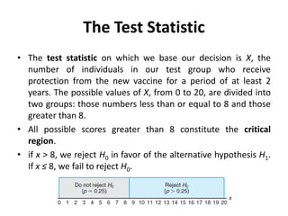
The Test Statistic
•The test statistic on which we base our decision is X, the
number of individuals in our test group who receive
protection from the new vaccine for a period of at least 2
years. The possible values of X, from 0 to 20, are divided into
two groups: those numbers less than or equal to 8 and those
greater than 8.
• All possible scores greater than 8 constitute the critical
region.
• if x > 8, we reject H0 in favor of the alternative hypothesis H1.
If x ≤ 8, we fail to reject H0.
11.
Types of Error
•Rejection of the null hypothesis when it is true
is called a type I error.
• Non-rejection of the null hypothesis when it is
false is called a type II error.
12.
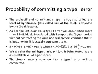
Probability of committinga type I error
• The probability of committing a type I error, also called the
level of significance (also called size of the test), is denoted
by the Greek letter α.
• As per the last example, a type I error will occur when more
than 8 individuals inoculated with B surpass the 2-year period
without contracting the virus and researchers conclude that B
is better when it is actually equivalent to A.
• α = P(type I error) = P (X >8 when p =1/4)= 𝑏(𝑋, 20,
1
4
)
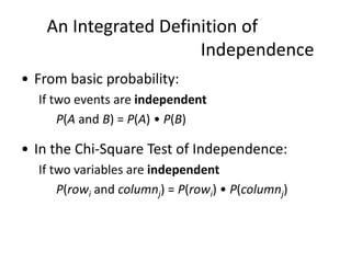
20
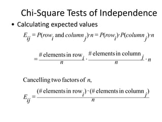
𝑥=9 =0.0409
• We say that the null hypothesis, p = 1/4, is being tested at the
α = 0.0409 level of significance.
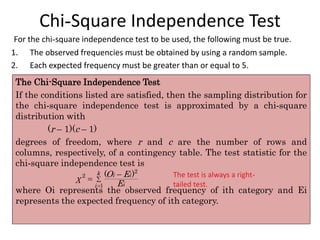
• Therefore chance is very low that a type I error will be
committed.
13.
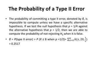
The Probability ofa Type II Error
• The probability of committing a type II error, denoted by β, is
impossible to compute unless we have a specific alternative
hypothesis. If we test the null hypothesis that p = 1/4 against
the alternative hypothesis that p = 1/2, then we are able to
compute the probability of not rejecting H0 when it is false.
• β = P(type II error) = P (X ≤ 8 when p =1/2)= 𝑏(𝑥, 20,
1
2
)
8
𝑥=0
= 0.2517
14.
• A realestate agent claims that 60% of all private residences being
built today are 3-bedroom homes. To test this claim, a large sample
of new residences is inspected; the proportion of these homes with
3 bedrooms is recorded and used as the test statistic. State the null
and alternative hypotheses to be used in this test.
• If the test statistic were substantially higher or lower than p = 0.6,
we would reject the agent’s claim. Hence, we should make the
hypothesis
H0: p = 0.6,
H1: p != 0.6.
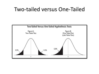
• The alternative hypothesis implies a two-tailed test with the critical
region divided equally in both tails of the distribution of P, our test
statistic.
15.
The Use ofP-Values for Decision Making in
Testing Hypotheses
• In testing hypotheses in which the test statistic is discrete, the
critical region may be chosen arbitrarily and its size determined. If α
is too large, it can be reduced by making an adjustment in the
critical value.
• Over a number of generations of statistical analysis, it had
become customary to choose an α of 0.05 or 0.01 and select the
critical region accordingly.
• if the test is two tailed and α is set at the 0.05 level of significance
and the test statistic involves, say, the standard normal distribution,
then a z-value is observed from the data and the critical region is z >
1.96 or z < −1.96,
• A value of z in the critical region prompts the statement “The value
of the test statistic is significant”
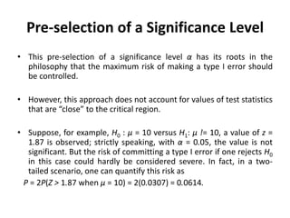
Pre-selection of aSignificance Level
• This pre-selection of a significance level α has its roots in the
philosophy that the maximum risk of making a type I error should
be controlled.
• However, this approach does not account for values of test statistics
that are “close” to the critical region.
• Suppose, for example, H0 : μ = 10 versus H1: μ != 10, a value of z =
1.87 is observed; strictly speaking, with α = 0.05, the value is not
significant. But the risk of committing a type I error if one rejects H0
in this case could hardly be considered severe. In fact, in a two-
tailed scenario, one can quantify this risk as
P = 2P(Z > 1.87 when μ = 10) = 2(0.0307) = 0.0614.
18.
• The P-valueapproach has been adopted extensively by users
of applied statistics. The approach is designed to give the
user an alternative (in terms of a probability) to a mere
“reject” or “do not reject” conclusion.
19.
Testing Hypotheses
1. Identifythe population, distribution, inferential test
2. State the null and alternative hypotheses
3. Determine characteristics of the distribution
4. Determine critical values or cutoffs
5. Calculate test statistic (e.g., z statistic)
6. Make a decision
Z-test
• A Z-testis any statistical test for which the distribution of
the test statistic can be approximated by a normal
distribution.
• Z-test tests the mean of a distribution in which we already
know the population variance σ2 .
• For each significance level, the Z-test has a single critical value
(for example, 1.96 for 5% two tailed) which makes it more
convenient
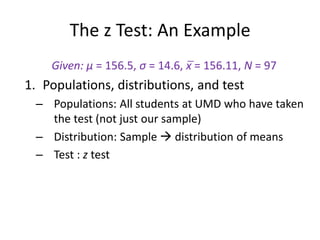
The z Test:An Example
Given: μ = 156.5, σ = 14.6, x̅ = 156.11, N = 97
1. Populations, distributions, and test
– Populations: All students at UMD who have taken
the test (not just our sample)
– Distribution: Sample distribution of means
– Test : z test
24.
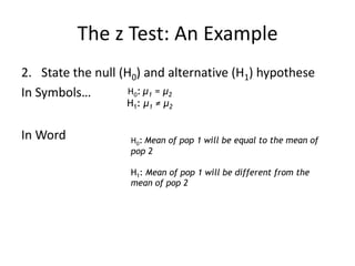
The z Test:An Example
2. State the null (H0) and alternative (H1) hypothese
In Symbols…
In Word
H0: μ1 = μ2
H1: μ1 ≠ μ2
H0: Mean of pop 1 will be equal to the mean of
pop 2
H1: Mean of pop 1 will be different from the
mean of pop 2
25.
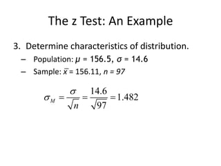
The z Test:An Example
3. Determine characteristics of distribution.
– Population: μ = 156.5, σ = 14.6
– Sample: x̅ = 156.11, n = 97
14.6
1.482
97
M
n
26.
The z Test:An Example
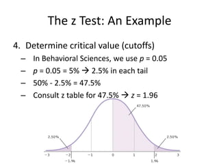
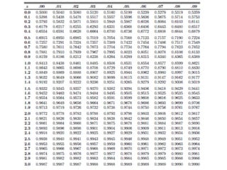
4. Determine critical value (cutoffs)
– In Behavioral Sciences, we use p = 0.05
– p = 0.05 = 5% 2.5% in each tail
– 50% - 2.5% = 47.5%
– Consult z table for 47.5% z = 1.96
28.
The z Test:An Example
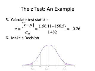
5. Calculate test statistic
6. Make a Decision
(156.11 156.5)
0.26
1.482
M
x
z
29.
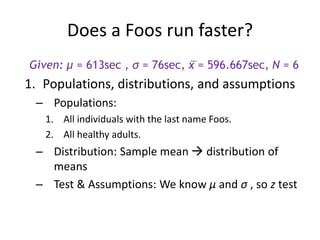
Does a Foosrun faster?
• When I was growing up my father told me that our last name, Foos, was
German for foot (Fuβ) because our ancestors had been very fast runners. I
am curious whether there is any evidence for this claim in my family so I
have gathered running times for a distance of one mile from 6 family
members. The average healthy adult can run one mile in 10 minutes and
13 seconds (standard deviation of 76 seconds). Is my family running speed
different from the national average? Assume that running speed follows a
normal distribution.
Person Running Time
Paul 13min 48sec
Phyllis 10min 10sec
Tom 7min 54sec
Aleigha 9min 22sec
Arlo 8min 38sec
David 9min 48sec
…in seconds
828sec
610sec
474sec
562sec
518sec
588sec
∑ = 3580
N = 6
M = 596.667
30.
Does a Foosrun faster?
Given: μ = 613sec , σ = 76sec, x̅ = 596.667sec, N = 6
1. Populations, distributions, and assumptions
– Populations:
1. All individuals with the last name Foos.
2. All healthy adults.
– Distribution: Sample mean distribution of
means
– Test & Assumptions: We know μ and σ , so z test
31.
Given: μ =613sec , σ = 76sec, x̅ = 596.667sec, N = 6
2. State the null (H0) and research (H1)hypotheses
H0: People with the last name Foos do not run at different
speeds than the national average.
H1: People with the last name Foos do run at different
speeds (either slower or faster) than the national
average.
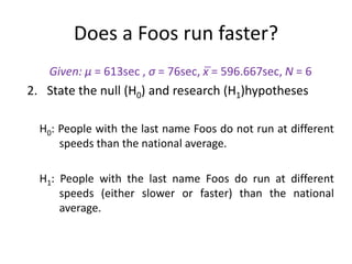
Does a Foos run faster?
32.
Does a Foosrun faster?
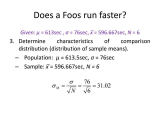
Given: μ = 613sec , σ = 76sec, x̅ = 596.667sec, N = 6
3. Determine characteristics of comparison
distribution (distribution of sample means).
– Population: μ = 613.5sec, σ = 76sec
– Sample: x̅ = 596.667sec, N = 6
76
31.02
6
M
N
33.
Does a Foosrun faster?
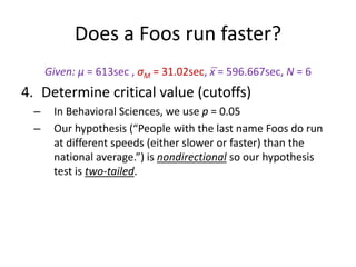
Given: μ = 613sec , σM = 31.02sec, x̅ = 596.667sec, N = 6
4. Determine critical value (cutoffs)
– In Behavioral Sciences, we use p = 0.05
– Our hypothesis (“People with the last name Foos do run
at different speeds (either slower or faster) than the
national average.”) is nondirectional so our hypothesis
test is two-tailed.
34.
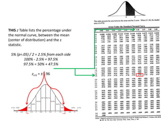
THIS z Tablelists the percentage under
the normal curve, between the mean
(center of distribution) and the z
statistic.
5% (p=.05) / 2 = 2.5% from each side
100% - 2.5% = 97.5%
97.5% = 50% + 47.5%
zcrit = ±1.96
+1.96
-1.96
35.
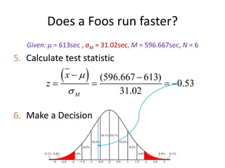
Does a Foosrun faster?
Given: μ = 613sec , σM = 31.02sec, M = 596.667sec, N = 6
5. Calculate test statistic
6. Make a Decision
(596.667 613)
0.53
31.02
M
x
z
36.
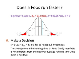
Does a Foosrun faster?
Given: μ = 613sec , σM = 31.02sec, x̅ = 596.667sec, N = 6
6. Make a Decision
z = 0-.53 < zcrit = ±1.96, fail to reject null hypothesis
The average one mile running time of Foos family members
is not different from the national average running time…the
myth is not true
37.
• A randomsample of 100 recorded deaths in the United States
during the past year showed an average life span of 71.8
years. Assuming a population standard deviation of 8.9 years,
does this seem to indicate that the mean life span today is
greater than 70 years? Use a 0.05 level of significance.
38.
• Population: Citizenof USA who died
• Distribution: Mean distribution of sample
• Test: Z test
• Hypothesis:
• H0: μ = 70 years.
• H1: μ > 70 years.
• Critical region: z > 1.645, (α = 0.05, one tailed
test)
39.
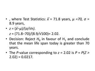
• , whereTest Statistics: x̅ = 71.8 years, μ =70, σ =
8.9 years,
• z = (x̅−μ)/(σ/√n).
z = (71.8−70)/(8.9/√100)= 2.02.
• Decision: Reject H0 in favour of H1 and conclude
that the mean life span today is greater than 70
years.
• The P-value corresponding to z = 2.02 is P = P(Z >
2.02) = 0.0217.
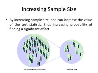
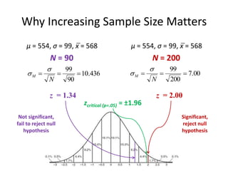
Increasing Sample Size
•By increasing sample size, one can increase the value
of the test statistic, thus increasing probability of
finding a significant effect
42.
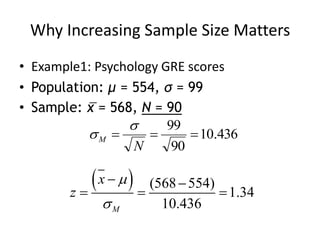
Why Increasing SampleSize Matters
• Example1: Psychology GRE scores
• Population: μ = 554, σ = 99
• Sample: x̅ = 568, N = 90
436
.
10
90
99
N
M
(568 554)
1.34
10.436
M
x
z
43.
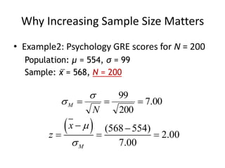
Why Increasing SampleSize Matters
• Example2: Psychology GRE scores for N = 200
Population: μ = 554, σ = 99
Sample: x̅ = 568, N = 200
00
.
7
200
99
N
M
(568 554)
2.00
7.00
M
x
z
44.
Why Increasing SampleSize Matters
μ = 554, σ = 99, x̅ = 568
N = 90
μ = 554, σ = 99, x̅ = 568
N = 200
436
.
10
90
99
N
M
00
.
7
200
99
N
M
z = 1.34 z = 2.00
zcritical (p=.05) = ±1.96
Not significant,
fail to reject null
hypothesis
Significant,
reject null
hypothesis
45.
One Sample: Teston a Single
Proportion
• A builder claims that heat pumps are installed in 70% of all
homes being constructed today in the city of Richmond,
Virginia. Would you agree with this claim if a random survey
of new homes in this city showed that 8 out of 15 had heat
pumps installed? Use a 0.10 level of significance.
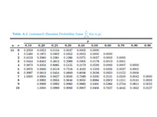
47.
• H0: p= 0.7.
• H1: p != 0.7.
• α = 0.10
• Test statistic: Binomial variable X with p = 0.7 and n = 15.
Computations: x = 8 and mean(np) = (15)(0.7) = 10.5.
• P=P(X ≤ 8 when p = 0.7) + P(X≥13 when p = 0.7)
• = 2P(X ≤ 8 when p = 0.7) =2 𝑏 𝑥; 15,0.7 = 0.2622 > 0.1
8
𝑥=0
• Decision: Do not reject H0. Conclude that there is insufficient
evidences to doubt the builder’s claim.
48.
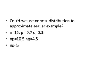
• Could weuse normal distribution to
approximate earlier example?
• n=15, p =0.7 q=0.3
• np=10.5 nq=4.5
• nq<5
49.
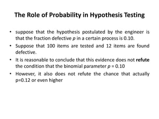
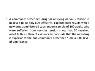
• A commonlyprescribed drug for relieving nervous tension is
believed to be only 60% effective. Experimental results with a
new drug administered to a random sample of 100 adults who
were suffering from nervous tension show that 70 received
relief. Is this sufficient evidence to conclude that the new drug
is superior to the one commonly prescribed? Use a 0.05 level
of significance.
51.
• H0: p= 0.6.
• H1: p > 0.6.
• α = 0.05.
• Critical region: z > 1.645 (one tailed test) [np and nq >5]
• Computations: x̅ = 70, n = 100, and
• z =(x̅ − np)/(√𝑛𝑝𝑞)
=(70-60 )/( 100 ∗ 0.6 ∗ 0.4)
= 1/( 0.24 =2.04,
Decision: Reject H0 and conclude that the new drug is superior
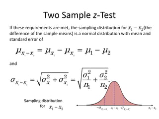
Two Sample z-Test
Ifthese requirements are met, the sampling distribution for (the
difference of the sample means) is a normal distribution with mean and
standard error of
1 2 1 2
1 2
x x x x
μ μ μ μ μ
1 2
x x
and
1 2 1 2
2 2
2 2 1 2
1 2
.
x x x x
σ σ
σ σ σ
n n
1 2
μ μ
1 2
x x
σ
1 2
x x
σ
Sampling distribution
for
1 2
x x
1 2
x x
54.
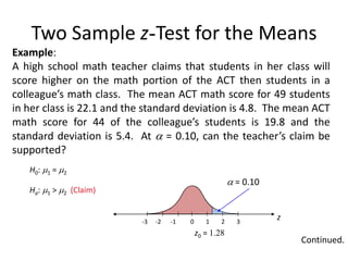
Two Sample z-Testfor the Means
Example:
A high school math teacher claims that students in her class will
score higher on the math portion of the ACT then students in a
colleague’s math class. The mean ACT math score for 49 students
in her class is 22.1 and the standard deviation is 4.8. The mean ACT
math score for 44 of the colleague’s students is 19.8 and the
standard deviation is 5.4. At = 0.10, can the teacher’s claim be
supported?
Ha: 1 > 2 (Claim)
H0: 1 = 2
Continued.
z0 = 1.28
z
0 1 2 3
-3 -2 -1
= 0.10
55.
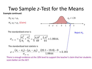
Two Sample z-Testfor the Means
1 2
1 2 1 2
x x
x x μ μ
z
σ
Example continued:
The standardized error is
22.1 19.8 0
1.0644
Ha: 1 > 2 (Claim)
H0: 1 = 2
1 2
2 2
1 2
1 2
x x
σ σ
σ
n n
1.0644.
2 2
4.8 5.4
49 44
The standardized test statistic is
2.161
z0 = 1.28
z
0 1 2 3
-3 -2 -1
Reject H0.
There is enough evidence at the 10% level to support the teacher’s claim that her students
score better on the ACT.
56.
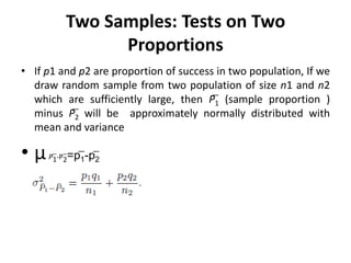
Two Samples: Testson Two
Proportions
• If p1 and p2 are proportion of success in two population, If we
draw random sample from two population of size n1 and n2
which are sufficiently large, then P1̅ (sample proportion )
minus P2̅ will be approximately normally distributed with
mean and variance
• µP1̅-P2̅=p1̅-p2̅
57.
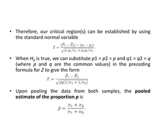
• Therefore, ourcritical region(s) can be established by using
the standard normal variable
• When H0 is true, we can substitute p1 = p2 = p and q1 = q2 = q
(where p and q are the common values) in the preceding
formula for Z to give the form
• Upon pooling the data from both samples, the pooled
estimate of the proportion p is
58.
• A voteis to be taken among the residents of a town and the
surrounding county to determine whether a proposed
chemical plant should be constructed. The construction site is
within the town limits, and for this reason many voters in the
county believe that the proposal will pass because of the large
proportion of town voters who favor the construction. To
determine if there is a significant difference in the proportions
of town voters and county voters favoring the proposal, a poll
is taken. If 120 of 200 town voters favor the proposal and 240
of 500 county residents favor it, would you agree that the
proportion of town voters favoring the proposal is higher than
the proportion of county voters? Use an α = 0.05 level of
significance.
59.
• Let p1and p2 be the true proportions of voters in the town
and county, respectively, favoring the proposal.
• H0: p1 = p2.
• H1: p1 > p2.
• α = 0.05.
• Critical region: z > 1.645 (one tailed)
• In lastfew scenarios that we explained, it was assumed that
the population standard deviation is known. This assumption
may not be unreasonable in situations where the engineer is
quite familiar with the system or process.
• However, in many experimental scenarios, knowledge of σ is
certainly no more reasonable than knowledge of the
population mean μ. Often, in fact, an estimate of σ must be
supplied by the same sample information that produced the
sample average x̅.
62.
Using Samples toEstimate Population
Variability
• Acknowledge error
• Smaller samples, less spread
2
( )
1
i
X X
s
N
63.
What is aT-distribution?
• A t-distribution is like a Z distribution, except has slightly fatter tails
to reflect the uncertainty added by estimating .
• The bigger the sample size (i.e., the bigger the sample size used to
estimate ), then the closer t becomes to Z.
• If n>=30, t approaches Z.
• Let X1,X2, . . . , Xn be independent random variables that are all
normal with mean μ and standard deviation σ. Let
X̅= 𝑋𝑖
𝑛
𝑖 and S2=
1
𝑛−1
𝑋𝑖 − 𝑋 2
𝑛
𝑖=1
• Then the random variable T =
𝑋−µ
𝑆/√𝑛
has a t-distribution with v = n − 1
degrees of freedom.
64.
What happened toσM?
• We have a new measure of standard deviation for a
sample mean distribution or standard error of the mean
(SEM) (as opposed to a population):
– We need a new measure of standard error based on sample
standard deviation:
– Wait, what happened to “N-1”?
– We already did that when we calculated s, don’t correct again!
N
s
sM
65.
Degrees of Freedom
•The number of scores that are free to vary when
estimating a population parameter from a sample
– df = N – 1 (for a Single-Sample t Test)
66.
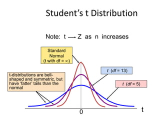
Student’s t Distribution
t
0
t(df = 5)
t (df = 13)
t-distributions are bell-
shaped and symmetric, but
have ‘fatter’ tails than the
normal
Standard
Normal
(t with df = )
Note: t Z as n increases
67.
Single-Sample t Test:Attendance in
Therapy Sessions
• Our Counseling center on campus is concerned that most students
requiring therapy do not take advantage of their services. Right
now students attend only 4.6 sessions in a given year!
Administrators are considering having patients sign a contract
stating they will attend at least 10 sessions in an academic year.
• Question: Does signing the contract actually increase
participation/attendance?
• We had 5 patients who signed the contract and we counted the
number of times they attended therapy sessions
Number of Attended Therapy Sessions
6
6
12
7
8
68.
Single-Sample t Test:Attendance in
Therapy Sessions
1. Identify
– Populations:
• Pop 1: All clients who sign contract
• Pop 2: All clients who do not sign contract
– Distribution:
• One Sample mean: Distribution of sample means of
pop2
– Test & Assumptions: Population mean is known but not
standard deviation single-sample t test
69.
Single-Sample t Test:Attendance in
Therapy Sessions
2. State the null and research hypotheses
H0: Clients who sign the contract will attend the same number
of sessions as those who do not sign the contract.
H1: Clients who sign the contract will attend a different
number of sessions than those who do not sign the
contract.
70.
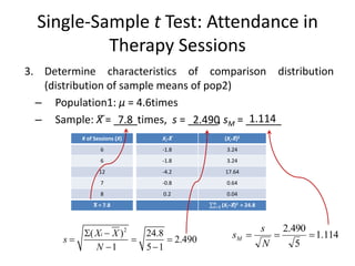
Single-Sample t Test:Attendance in
Therapy Sessions
3. Determine characteristics of comparison distribution
(distribution of sample means of pop2)
– Population1: μ = 4.6times
– Sample: X̅ = ____times, s = _____, sM = ______
2
( ) 24.8
2.490
1 5 1
i
X X
s
N
114
.
1
5
490
.
2
N
s
sM
# of Sessions (X)
6
6
12
7
8
X̅ = 7.8
Xi-X̅
-1.8
-1.8
-4.2
-0.8
0.2
(Xi-X̅)2
3.24
3.24
17.64
0.64
0.04
(Xi−X̅)2
𝒏
𝒊=𝟏 = 24.8
7.8 2.490 1.114
71.
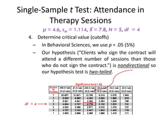
Single-Sample t Test:Attendance in
Therapy Sessions
μ = 4.6, sM = 1.114, X̅ = 7.8, N = 5, df = 4
4. Determine critical value (cutoffs)
– In Behavioral Sciences, we use p = .05 (5%)
– Our hypothesis (“Clients who sign the contract will
attend a different number of sessions than those
who do not sign the contract.”) is nondirectional so
our hypothesis test is two-tailed.
df = 4
72.
Single-Sample t Test:Attendance in
Therapy Sessions
μ = 4.6, sM = 1.114, X̅ = 7.8, N = 5, df = 4
4. Determine critical value (cutoffs)
tcrit = ± 2.776
73.
Single-Sample t Test:Attendance in
Therapy Sessions
μM = 4.6, sM = 1.114, x̅ = 7.8, N = 5, df = 4
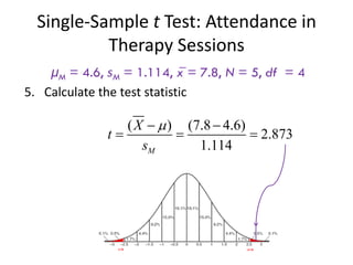
5. Calculate the test statistic
( ) (7.8 4.6)
2.873
1.114
M
X
t
s
+2.76
-2.76
74.
Single-Sample t Test:Attendance in
Therapy Sessions
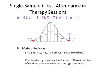
μ = 4.6, sM = 1.114, X̅ = 7.8, N = 5, df = 4
6. Make a decision
t = 2.873 > tcrit = ±2.776, reject the null hypothesis
Clients who sign a contract will attend different number
of sessions than those who do not sign a contract,
2.873
75.
More Problem:
• Amanufacturer of light bulbs claims that its light bulbs have a
mean life of 1520 hours with an unknown standard deviation.
A random sample of 40 such bulbs is selected for testing. If
the sample produces a mean value of 1505 hours and a
sample standard deviation of 86, is there sufficient evidence
to claim that the mean life is significantly less than the
manufacturer claimed?
– Assume that light bulb lifetimes are roughly normally distributed.
76.
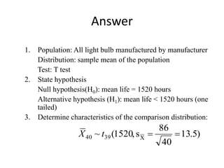
Answer
1. Population: Alllight bulb manufactured by manufacturer
Distribution: sample mean of the population
Test: T test
2. State hypothesis
Null hypothesis(H0): mean life = 1520 hours
Alternative hypothesis (H1): mean life < 1520 hours (one
tailed)
3. Determine characteristics of the comparison distribution:
)
5
.
13
40
86
s
,
1520
(
~ X
39
40
t
X
77.
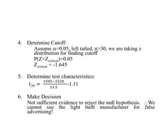
4. Determine Cutoff:
Assume=0.05, left tailed, n>30, we are taking z
distribution for finding cutoff
P(Z<Zcritical)=0.05
Zcritical = -1.645
5. Determine test characteristics:
𝑡39 =
1505−1520
13.5
=-1.11
6. Make Decision
Not sufficient evidence to reject the null hypothesis. We
cannot sue the light bulb manufacturer for false
advertising!
78.
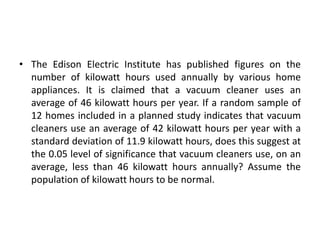
• The EdisonElectric Institute has published figures on the
number of kilowatt hours used annually by various home
appliances. It is claimed that a vacuum cleaner uses an
average of 46 kilowatt hours per year. If a random sample of
12 homes included in a planned study indicates that vacuum
cleaners use an average of 42 kilowatt hours per year with a
standard deviation of 11.9 kilowatt hours, does this suggest at
the 0.05 level of significance that vacuum cleaners use, on an
average, less than 46 kilowatt hours annually? Assume the
population of kilowatt hours to be normal.
80.
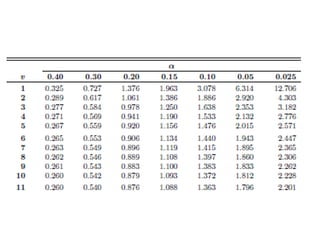
• H0: μ= 46 kilowatt hours.
• H1: μ < 46 kilowatt hours (one tailed, left tailed)
• α = 0.05.
• Critical region: t < −1.796, where 11 is degrees of
freedom (from table).
• Computations: t = (x̅−μ)/(s/√n) x̅ = 42, μ = 46 , s = 11.9
and n = 12.
• Hence, t =(42 − 46)/(11.9/√12)= −1.16,
• Decision: Do not reject H0 and conclude that the
average number of kilowatt hours used annually by
home vacuum cleaners is not significantly less than 46.
Two Sample t-Test
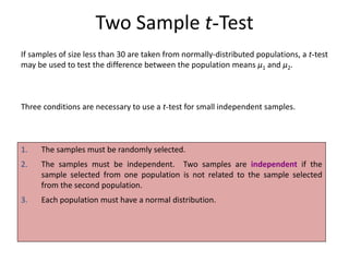
1.The samples must be randomly selected.
2. The samples must be independent. Two samples are independent if the
sample selected from one population is not related to the sample selected
from the second population.
3. Each population must have a normal distribution.
If samples of size less than 30 are taken from normally-distributed populations, a t-test
may be used to test the difference between the population means μ1 and μ2.
Three conditions are necessary to use a t-test for small independent samples.
83.
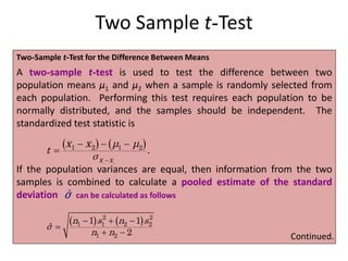
Two Sample t-Test
Two-Samplet-Test for the Difference Between Means
A two-sample t-test is used to test the difference between two
population means μ1 and μ2 when a sample is randomly selected from
each population. Performing this test requires each population to be
normally distributed, and the samples should be independent. The
standardized test statistic is
If the population variances are equal, then information from the two
samples is combined to calculate a pooled estimate of the standard
deviation can be calculated as follows
1 2
1 2 1 2
.
x x
x x μ μ
t
σ
ˆ
σ
2 2
1 1 2 2
1 2
1 1
ˆ
2
n s n s
σ
n n
Continued.
84.
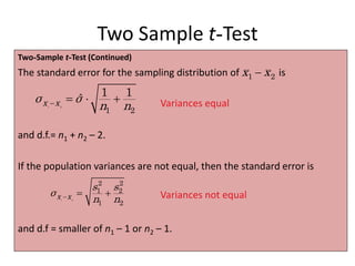
Two Sample t-Test
Two-Samplet-Test (Continued)
The standard error for the sampling distribution of is
and d.f.= n1 + n2 – 2.
If the population variances are not equal, then the standard error is
and d.f = smaller of n1 – 1 or n2 – 1.
1 2
1 2
1 1
ˆ
x x
σ σ
n n
1 2
x x
Variances equal
1 2
2 2
1 2
1 2
x x
s s
σ
n n
Variances not equal
85.
Two Sample t-Testfor the Means
1. State the claim mathematically.
Identify the null and alternative
hypotheses.
2. Specify the level of significance.
3. Identify the degrees of freedom
and sketch the sampling
distribution.
4. Determine the critical value(s).
Continued.
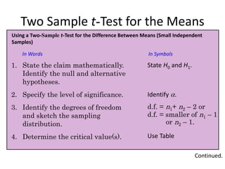
Using a Two-Sample t-Test for the Difference Between Means (Small Independent
Samples)
In Words In Symbols
State H0 and H1.
Identify .
Use Table
d.f. = n1+ n2 – 2 or
d.f. = smaller of n1 – 1
or n2 – 1.
86.
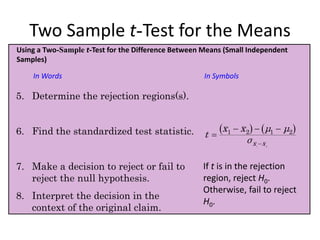
Two Sample t-Testfor the Means
In Words In Symbols
If t is in the rejection
region, reject H0.
Otherwise, fail to reject
H0.
5. Determine the rejection regions(s).
6. Find the standardized test statistic.
7. Make a decision to reject or fail to
reject the null hypothesis.
8. Interpret the decision in the
context of the original claim.
Using a Two-Sample t-Test for the Difference Between Means (Small Independent
Samples)
1 2
1 2 1 2
x x
x x μ μ
t
σ
87.
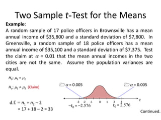
Two Sample t-Testfor the Means
Example:
A random sample of 17 police officers in Brownsville has a mean
annual income of $35,800 and a standard deviation of $7,800. In
Greensville, a random sample of 18 police officers has a mean
annual income of $35,100 and a standard deviation of $7,375. Test
the claim at = 0.01 that the mean annual incomes in the two
cities are not the same. Assume the population variances are
equal.
Ha: 1 2 (Claim)
H0: 1 = 2
Continued.
–t0 = –2.576
= 0.005
d.f. = n1 + n2 – 2
= 17 + 18 – 2 = 33
t0 = 2.576
t
0 1 2 3
-3 -2 -1
= 0.005
89.
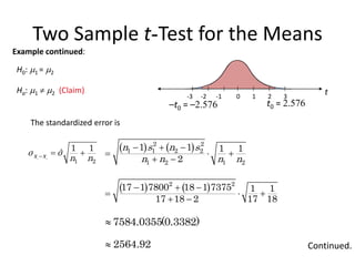
Two Sample t-Testfor the Means
Example continued:
The standardized error is
1 2
1 2
1 1
ˆ
x x
σ σ
n n
2 2
17 1 7800 18 1 7375 1 1
17 18 2 17 18
2 2
1 1 2 2
1 2 1 2
1 1 1 1
2
n s n s
n n n n
Ha: 1 2 (Claim)
H0: 1 = 2
–t0 = –2.576
t
0 1 2 3
-3 -2 -1
t0 = 2.576
7584.0355(0.3382)
Continued.
2564.92
90.
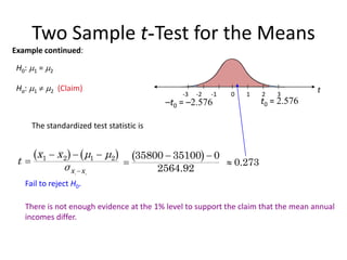
Two Sample t-Testfor the Means
1 2
1 2 1 2
x x
x x μ μ
t
σ
Example continued:
The standardized test statistic is
0.273
Fail to reject H0.
There is not enough evidence at the 1% level to support the claim that the mean annual
incomes differ.
Ha: 1 2 (Claim)
H0: 1 = 2
–t0 = –2.576
t
0 1 2 3
-3 -2 -1
t0 = 2.576
35800 35100 0
2564.92
91.
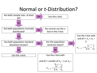
Normal or t-Distribution?
Areboth sample sizes at least
30?
Are both populations normally
distributed?
You cannot use the z-
test or the t-test.
No
Yes
Are both population standard
deviations known?
Use the z-test.
Yes
No
Are the population
variances equal?
Use the z-test. Use the t-test with
and d.f = smaller of n1 – 1 or n2 –
1.
1 2
2 2
1 2
1 2
x x
s s
σ
n n
Use the t-test with
and d.f = n1 + n2 –
2.
1 2
1 2
1 1
ˆ
x x
σ σ
n n
Yes
No
No
Yes
92.
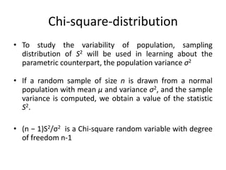
Chi-square-distribution
• To studythe variability of population, sampling
distribution of S2 will be used in learning about the
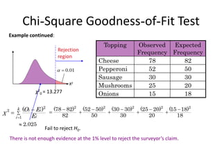
parametric counterpart, the population variance σ2
• If a random sample of size n is drawn from a normal
population with mean μ and variance σ2, and the sample
variance is computed, we obtain a value of the statistic
S2.
• (n − 1)S2/σ2 is a Chi-square random variable with degree
of freedom n-1
93.
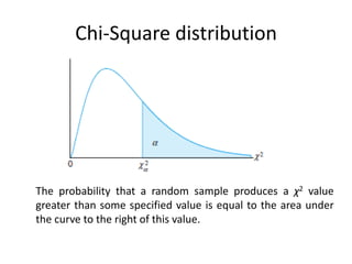
Chi-Square distribution
The probabilitythat a random sample produces a χ2 value
greater than some specified value is equal to the area under
the curve to the right of this value.
• A manufacturerof car batteries claims that the life of the
company’s batteries is approximately normally distributed
with a standard deviation equal to 0.9 year. If a random
sample of 10 of these batteries has a standard deviation of 1.2
years, do you think that σ > 0.9 year? Use a 0.05 level of
significance.
• H0: σ2 = 0.81.
• H1: σ2 > 0.81.
• α = 0.05.
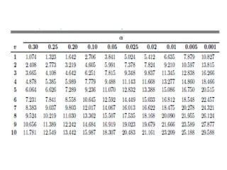
97.
• Critical region:From Figure we see that the null hypothesis is
rejected when χ2 > 16.919, χ2 = (n−1)s2/σ0
2
• Computations: s2 = 1.44 (as σ0 =1.2 given), n = 10, and
• χ2 =(9)(1.44)/0.81= 16.0
• Decision: The χ2-statistic is not significant at the 0.05 level.
98.
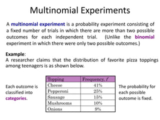
Multinomial Experiments
A multinomialexperiment is a probability experiment consisting of
a fixed number of trials in which there are more than two possible
outcomes for each independent trial. (Unlike the binomial
experiment in which there were only two possible outcomes.)
Example:
A researcher claims that the distribution of favorite pizza toppings
among teenagers is as shown below.
Topping Frequency, f
Cheese 41%
Pepperoni 25%
Sausage 15%
Mushrooms 10%
Onions 9%
Each outcome is
classified into
categories.
The probability for
each possible
outcome is fixed.
99.
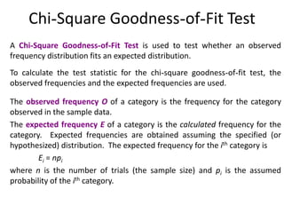
Chi-Square Goodness-of-Fit Test
AChi-Square Goodness-of-Fit Test is used to test whether an observed
frequency distribution fits an expected distribution.
To calculate the test statistic for the chi-square goodness-of-fit test, the
observed frequencies and the expected frequencies are used.
The observed frequency O of a category is the frequency for the category
observed in the sample data.
The expected frequency E of a category is the calculated frequency for the
category. Expected frequencies are obtained assuming the specified (or
hypothesized) distribution. The expected frequency for the ith category is
Ei = npi
where n is the number of trials (the sample size) and pi is the assumed
probability of the ith category.
100.
Observed and ExpectedFrequencies
Example:
200 teenagers are randomly selected and asked what their favorite
pizza topping is. The results are shown below. Find the observed
frequencies and the expected frequencies.
Topping Observed
Results
(n = 200)
Expected
% of
teenagers
Cheese 78 41%
Pepperoni 52 25%
Sausage 30 15%
Mushrooms 25 10%
Onions 15 9%
Observed
Frequency
78
52
30
25
15
Expected
Frequency
200(0.41) = 82
200(0.25) = 50
200(0.15) = 30
200(0.10) = 20
200(0.09) = 18
101.
Chi-Square Goodness-of-Fit Test
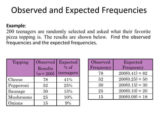
Forthe chi-square goodness-of-fit test to be used, the following must be true.
1. The observed frequencies must be obtained by using a random sample.
2. Each expected frequency must be greater than or equal to 5.
The Chi-Square Goodness-of-Fit Test
If the conditions listed above are satisfied, then the sampling
distribution for the goodness-of-fit test is approximated by a chi-
square distribution with k – 1 degrees of freedom, where k is the
number of categories. The test statistic for the chi-square goodness-of-
fit test is
where Oi represents the observed frequency of ith category and Ei
represents the expected frequency of ith category.
2
2
1
( )
k i i
i
i
O E
χ
E
The test is always a right-
tailed test.
103.
Chi-Square Goodness-of-Fit Test
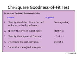
1.Identify the claim. State the null
and alternative hypotheses.
2. Specify the level of significance.
3. Identify the degrees of freedom.
4. Determine the critical value.
5. Determine the rejection region.
Continued.
Performing a Chi-Square Goodness-of-Fit Test
In Words In Symbols
State H0 and Ha.
Identify .
Use Table
d.f. = k – 1
104.
Chi-Square Goodness-of-Fit Test
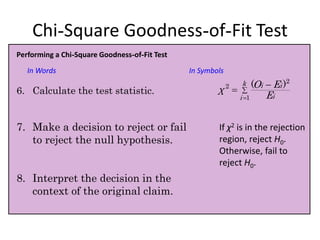
Performinga Chi-Square Goodness-of-Fit Test
In Words In Symbols
If χ2 is in the rejection
region, reject H0.
Otherwise, fail to
reject H0.
6. Calculate the test statistic.
7. Make a decision to reject or fail
to reject the null hypothesis.
8. Interpret the decision in the
context of the original claim.
2
2
1
( )
k i i
i
i
O E
χ
E
105.
Chi-Square Goodness-of-Fit Test
Example:
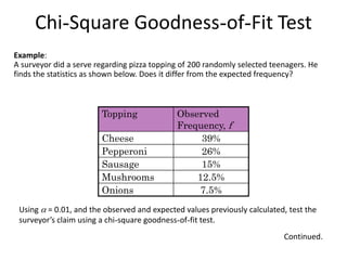
Asurveyor did a serve regarding pizza topping of 200 randomly selected teenagers. He
finds the statistics as shown below. Does it differ from the expected frequency?
Topping Observed
Frequency, f
Cheese 39%
Pepperoni 26%
Sausage 15%
Mushrooms 12.5%
Onions 7.5%
Continued.
Using = 0.01, and the observed and expected values previously calculated, test the
surveyor’s claim using a chi-square goodness-of-fit test.
106.
Chi-Square Goodness-of-Fit Test
Examplecontinued:
Continued.
Ha: observed frequency differs from expected frequency.
H0: observed and expected frequency does not differ. (Claim)
Because there are 5 categories, the chi-square distribution has k – 1 = 5 – 1 = 4 degrees of
freedom.
With d.f. = 4 and = 0.01, the critical value is χ2
0 = 13.277.
107.
Chi-Square Goodness-of-Fit Test
Examplecontinued:
Topping Observed
Frequency
Expected
Frequency
Cheese 78 82
Pepperoni 52 50
Sausage 30 30
Mushrooms 25 20
Onions 15 18
X2
0.01
Rejection
region
χ2
0 = 13.277
2
(78 82)
82
2
(52 50)
50
2
(30 30)
30
2
(25 20)
20
2
(15 18)
18
2.025
Fail to reject H0.
There is not enough evidence at the 1% level to reject the surveyor’s claim.
2
2
1
( )
k i i
i
i
O E
χ
E
108.
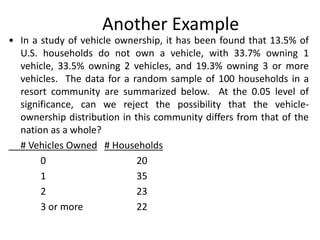
Another Example
• Ina study of vehicle ownership, it has been found that 13.5% of
U.S. households do not own a vehicle, with 33.7% owning 1
vehicle, 33.5% owning 2 vehicles, and 19.3% owning 3 or more
vehicles. The data for a random sample of 100 households in a
resort community are summarized below. At the 0.05 level of
significance, can we reject the possibility that the vehicle-
ownership distribution in this community differs from that of the
nation as a whole?
# Vehicles Owned # Households
0 20
1 35
2 23
3 or more 22
109.
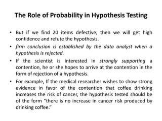
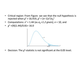
Goodness-of-Fit: An Example
I
H0:Observed distribution in this community is the same as it is
in the nation as a whole.
H1: Vehicle-ownership distribution in this community is not the
same as it is in the nation as a whole.
# Vehicles Oj Ej [Oj– Ej ]2/ Ej
0 20 13.5 3.1296
1 35 33.7 0.0501
2 23 33.5 3.2910
3+ 22 19.3 0.3777
Sum = 6.8484
110.
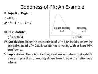
Goodness-of-Fit: An Example
II.Rejection Region:
= 0.05
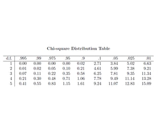
df = k – 1 = 4 – 1 = 3
III. Test Statistic:
c2 = 6.8484
IV. Conclusion: Since the test statistic of c2 = 6.8484 falls below the
critical value of c2 = 7.815, we do not reject H0 with at least 95%
confidence.
V. Implications: There is not enough evidence to show that vehicle
ownership in this community differs from that in the nation as a
whole.
0.05
0.95
Do Not Reject H
0 Reject H0
c =7.815
2
Chi-Square Independence Test
Achi-square independence test is used to test the independence
of two variables. Using a chi-square test, you can determine
whether the occurrence of one variable affects the probability of
the occurrence of the other variable.
114.
Contingency Tables
An r c contingency table shows the observed frequencies for two
variables. The observed frequencies are arranged in r rows and c
columns. The intersection of a row and a column is called a cell.
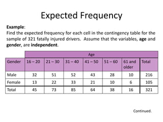
The following contingency table shows a random sample of 321 fatally
injured passenger vehicle drivers by age and gender. (Adapted from
Insurance Institute for Highway Safety)
6
10
21
33
22
13
Female
10
28
43
52
51
32
Male
61 and older
51 – 60
41 – 50
31 – 40
21 – 30
16 – 20
Gender
Age
115.
An Integrated Definitionof
Independence
• From basic probability:
If two events are independent
P(A and B) = P(A) • P(B)
• In the Chi-Square Test of Independence:
If two variables are independent
P(rowi and columnj) = P(rowi) • P(columnj)
116.
Chi-Square Tests ofIndependence
• Calculating expected values
n
j
i
ij
E
n
n
n
j
n
i
n
j
column
P
i
row
P
n
j
column
i
row
P
ij
E
)
column
in
elements
#
(
)
row
in
elements
(#
,
of
factors
two
Cancelling
column
in
elements
#
row
in
elements
#
)
(
)
(
)
and
(
117.
Expected Frequency
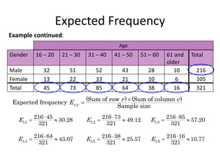
Example:
Find theexpected frequency for each cell in the contingency table for the
sample of 321 fatally injured drivers. Assume that the variables, age and
gender, are independent.
105
6
10
21
33
22
13
Female
16
10
61 and
older
321
38
64
85
73
45
Total
216
28
43
52
51
32
Male
Total
51 – 60
41 – 50
31 – 40
21 – 30
16 – 20
Gender
Age
Continued.
118.
Expected Frequency
Example continued:
105
6
10
21
33
22
13
Female
16
10
61and
older
321
38
64
85
73
45
Total
216
28
43
52
51
32
Male
Total
51 – 60
41 – 50
31 – 40
21 – 30
16 – 20
Gender
Age
,
(Sum of row ) (Sum of column )
Expected frequency
Sample size
r c
r c
E
1,2
216 73
49.12
321
E
1,1
216 45
30.28
321
E
1,3
216 85
57.20
321
E
1,5
216 38
25.57
321
E
1,4
216 64
43.07
321
E
1,6
216 16
10.77
321
E
119.
Chi-Square Independence Test
TheChi-Square Independence Test
If the conditions listed are satisfied, then the sampling distribution for
the chi-square independence test is approximated by a chi-square
distribution with
(r – 1)(c – 1)
degrees of freedom, where r and c are the number of rows and
columns, respectively, of a contingency table. The test statistic for the
chi-square independence test is
where Oi represents the observed frequency of ith category and Ei
represents the expected frequency of ith category.
The test is always a right-
tailed test.
For the chi-square independence test to be used, the following must be true.
1. The observed frequencies must be obtained by using a random sample.
2. Each expected frequency must be greater than or equal to 5.
2
2
1
( )
k i i
i
i
O E
χ
E
120.
Chi-Square Independence Test
1.Identify the claim. State the null
and alternative hypotheses.
2. Specify the level of significance.
3. Identify the degrees of freedom.
4. Determine the critical value.
5. Determine the rejection region.
Continued.
Performing a Chi-Square Independence Test
In Words In Symbols
State H0 and Ha.
Identify .
Use Table
d.f. = (r – 1)(c – 1)
121.
Chi-Square Independence Test
Performinga Chi-Square Independence Test
In Words In Symbols
If χ2 is in the rejection
region, reject H0.
Otherwise, fail to
reject H0.
6. Calculate the test statistic.
7. Make a decision to reject or fail
to reject the null hypothesis.
8. Interpret the decision in the
context of the original claim.
2
2
1
( )
k i i
i
i
O E
χ
E
122.
Chi-Square Independence Test
Example:
Thefollowing contingency table shows a random sample of 321 fatally injured passenger
vehicle drivers by age and gender. The expected frequencies are displayed in
parentheses. At = 0.05, can you conclude that the drivers’ ages are related to gender
in such accidents?
105
6 (5.23)
10
(12.43)
21
(20.93)
33
(27.80)
22
(23.88)
13
(14.72)
Female
16
10
(10.77)
61 and
older
321
38
64
85
73
45
216
28
(25.57)
43
(43.07)
52
(57.20)
51
(49.12)
32
(30.28)
Male
Total
51 – 60
41 – 50
31 – 40
21 – 30
16 – 20
Gender
Age
123.
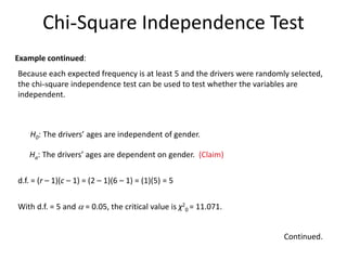
Chi-Square Independence Test
Examplecontinued:
Continued.
Ha: The drivers’ ages are dependent on gender. (Claim)
H0: The drivers’ ages are independent of gender.
Because each expected frequency is at least 5 and the drivers were randomly selected,
the chi-square independence test can be used to test whether the variables are
independent.
With d.f. = 5 and = 0.05, the critical value is χ2
0 = 11.071.
d.f. = (r – 1)(c – 1) = (2 – 1)(6 – 1) = (1)(5) = 5
124.
Chi-Square Independence Test
Examplecontinued:
X2
0.05
Rejection
region
χ2
0 = 11.071
5.23
12.43
20.93
27.80
23.88
14.72
10.77
25.57
43.07
57.20
49.12
30.28
E
0.77
2.43
0.07
5.2
1.88
1.72
0.77
2.43
0.07
5.2
1.88
1.72
O – E
0.201
2.9584
13
0.0551
0.5929
10
0.2309
5.9049
28
0.0001
0.0049
43
0.148
3.5344
22
0.4727
27.04
52
0.072
3.5344
51
0.0977
2.9584
32
0.5929
5.9049
0.0049
27.04
(O – E)2
0.1134
6
0.4751
10
0.0002
21
0.9727
33
O
2
( )
O E
E
2
2 ( )
2.84
O E
χ
E
Fail to reject H0.
There is not enough evidence at the 5% level to conclude that age is dependent on
gender in such accidents.


![• H0: p = 0.6.
• H1: p > 0.6.
• α = 0.05.
• Critical region: z > 1.645 (one tailed test) [np and nq >5]
• Computations: x̅ = 70, n = 100, and
• z =(x̅ − np)/(√𝑛𝑝𝑞)
=(70-60 )/( 100 ∗ 0.6 ∗ 0.4)
= 1/( 0.24 =2.04,
Decision: Reject H0 and conclude that the new drug is superior](https://image.slidesharecdn.com/10-260124141032-7be44b80/85/Inferential-statistics-a-branch-of-statistics-51-320.jpg)


![Goodness-of-Fit: An Example
I
H0: Observed distribution in this community is the same as it is
in the nation as a whole.
H1: Vehicle-ownership distribution in this community is not the
same as it is in the nation as a whole.
# Vehicles Oj Ej [Oj– Ej ]2/ Ej
0 20 13.5 3.1296
1 35 33.7 0.0501
2 23 33.5 3.2910
3+ 22 19.3 0.3777
Sum = 6.8484](https://image.slidesharecdn.com/10-260124141032-7be44b80/85/Inferential-statistics-a-branch-of-statistics-109-320.jpg)