index properties of soil 2.pptxioohfohof

Index properties of soil
3
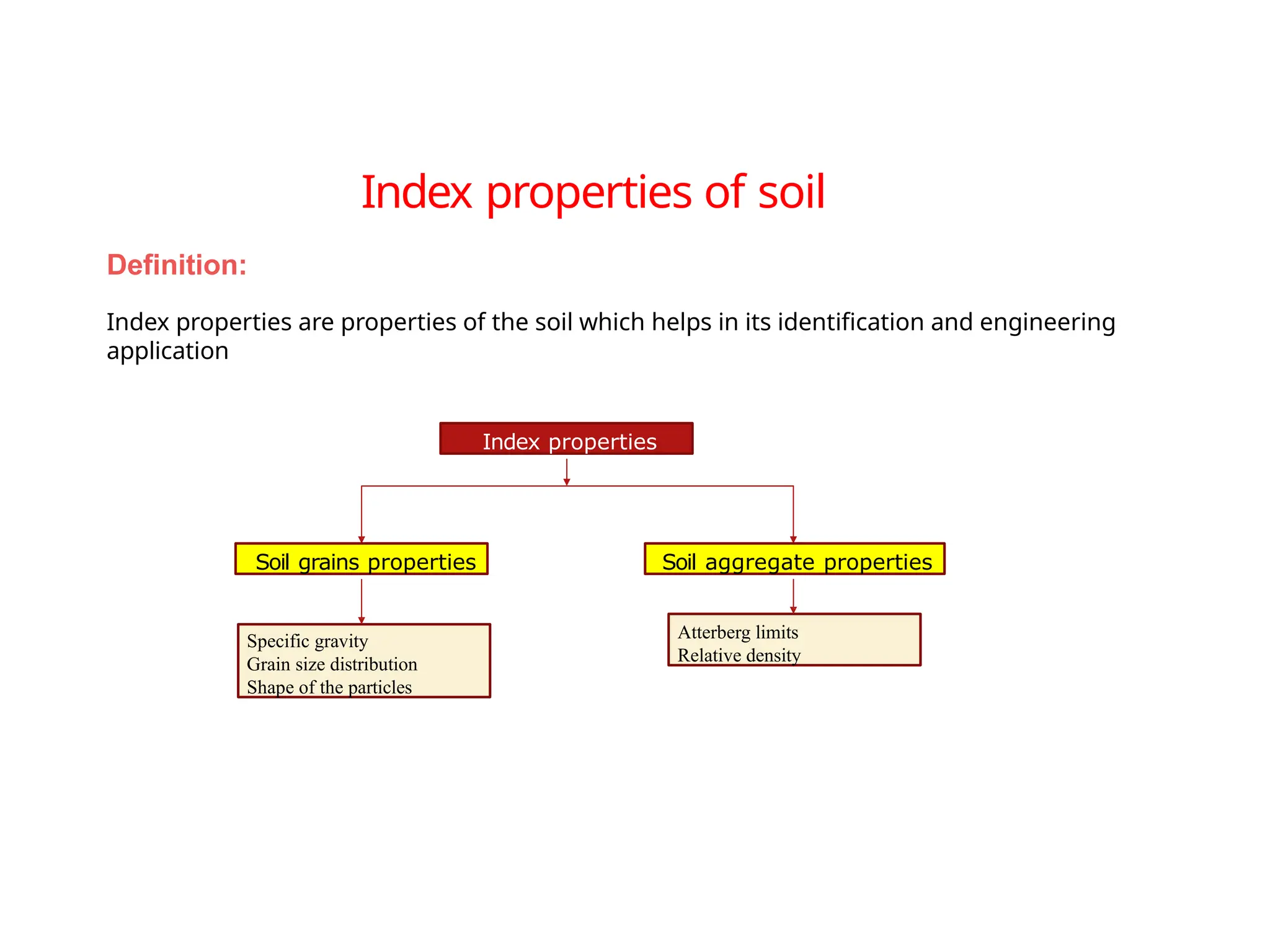
Definition:
Index properties are properties of the soil which helps in its identification and engineering
application.
Index properties
Soil grains properties Soil aggregate properties
Specific gravity
Grain size distribution
Shape of the particles
Atterberg limits
Relative density

3
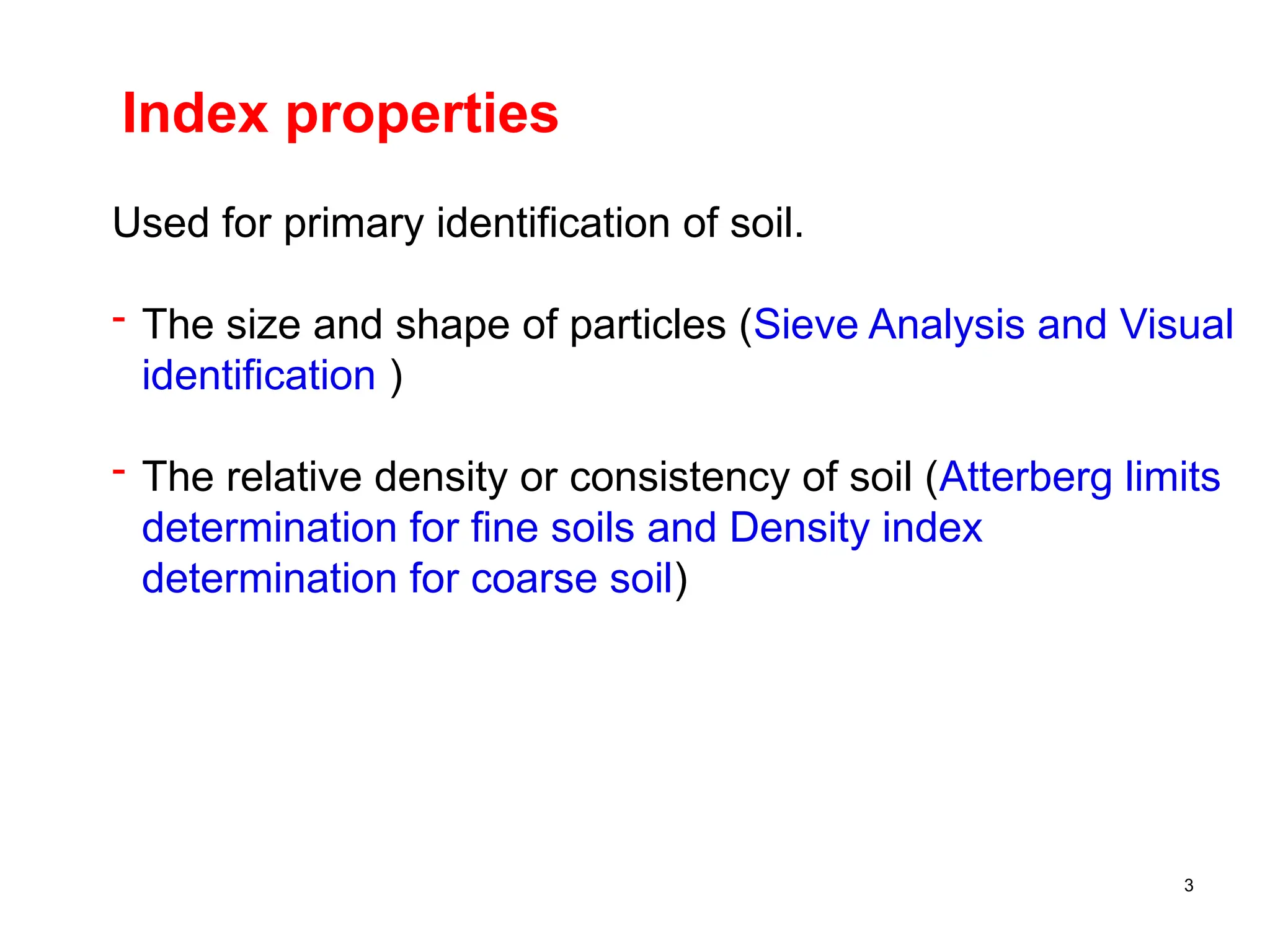
Index properties
Used for primary identification of soil.
- The size and shape of particles (Sieve Analysis and Visual
identification )
- The relative density or consistency of soil (Atterberg limits
determination for fine soils and Density index
determination for coarse soil)

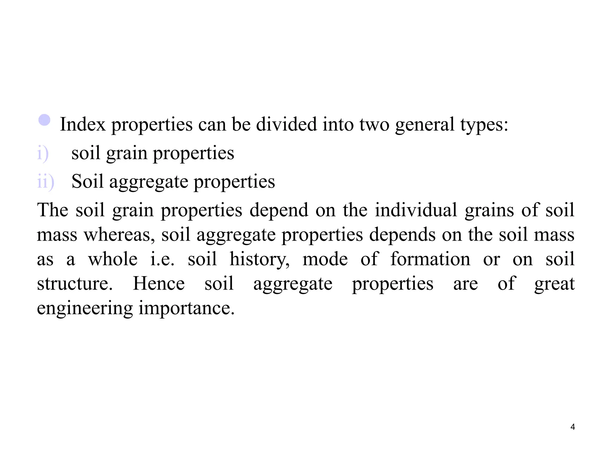
Index properties can be divided into two general types:
i) soil grain properties
ii) Soil aggregate properties
The soil grain properties depend on the individual grains of soil
mass whereas, soil aggregate properties depends on the soil mass
as a whole i.e. soil history, mode of formation or on soil
structure. Hence soil aggregate properties are of great
engineering importance.
4

Soil Grain Properties
The most important soil grain properties of soil are:
i) Grain Size Distribution: by sieve and sedimentation analysis
ii) Grain shape: Bulky, flaky and needle shaped etc.
5

Soil Aggregate Properties
a) Unconfined Compressive strength
b) Consistency and Atterberg’s Limits
c) Sensitivity
d) Thixotropy and Soil Activity
e) Relative Density
6

8
Major Soil Groups
0.002 200
63
2.36
0.075
Grain size (mm)
Boulder
Clay Silt Sand Gravel Cobble
Fine grain
soils
Coarse grain
soils
Granular soils or
Cohesionless soils
Cohesive
soils

11
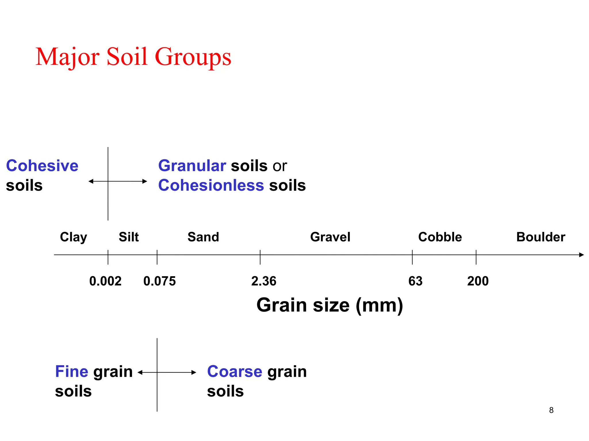
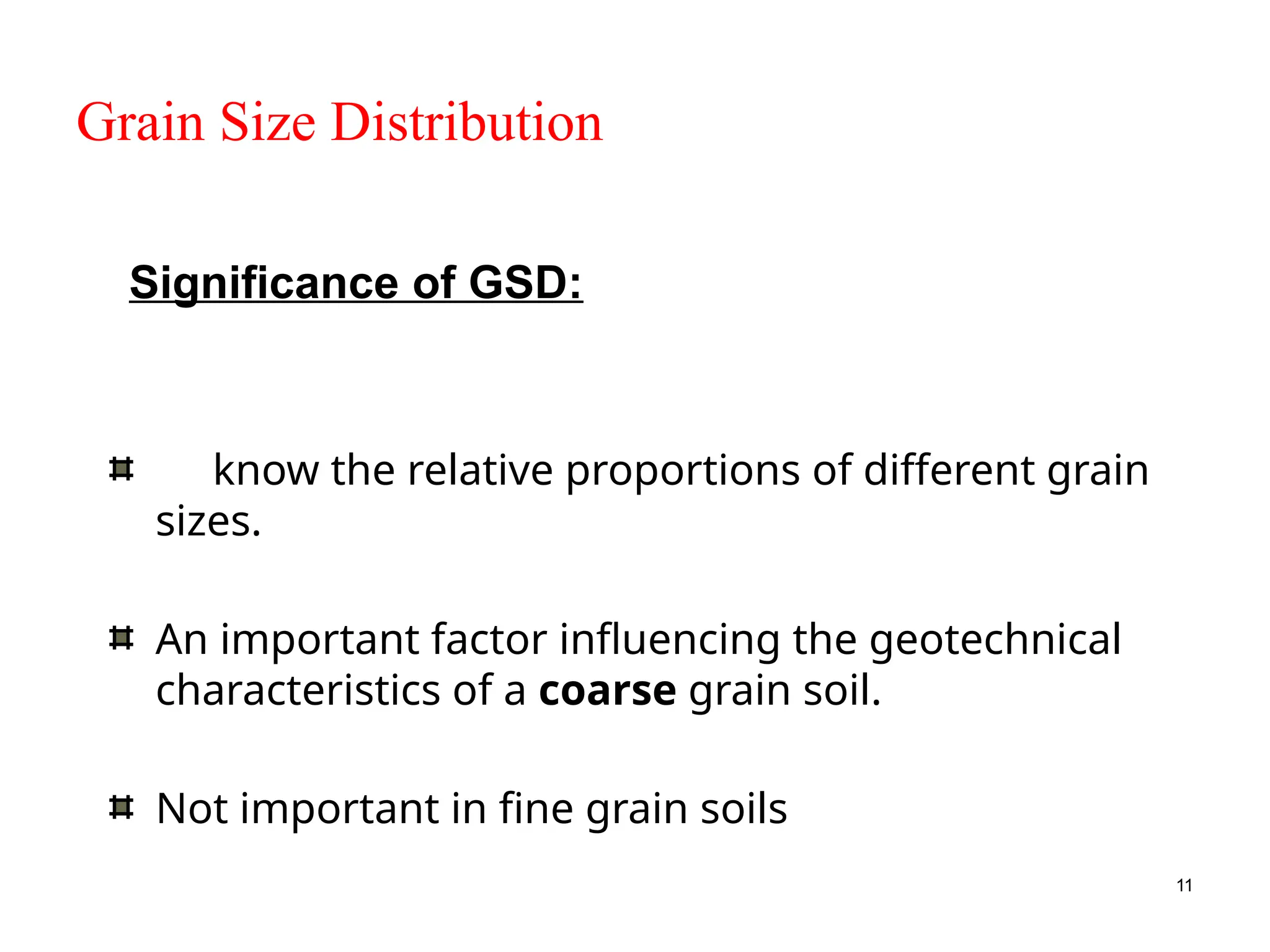
Grain Size Distribution
To know the relative proportions of different grain
sizes.
An important factor influencing the geotechnical
characteristics of a coarse grain soil.
Not important in fine grain soils
Significance of GSD:

12
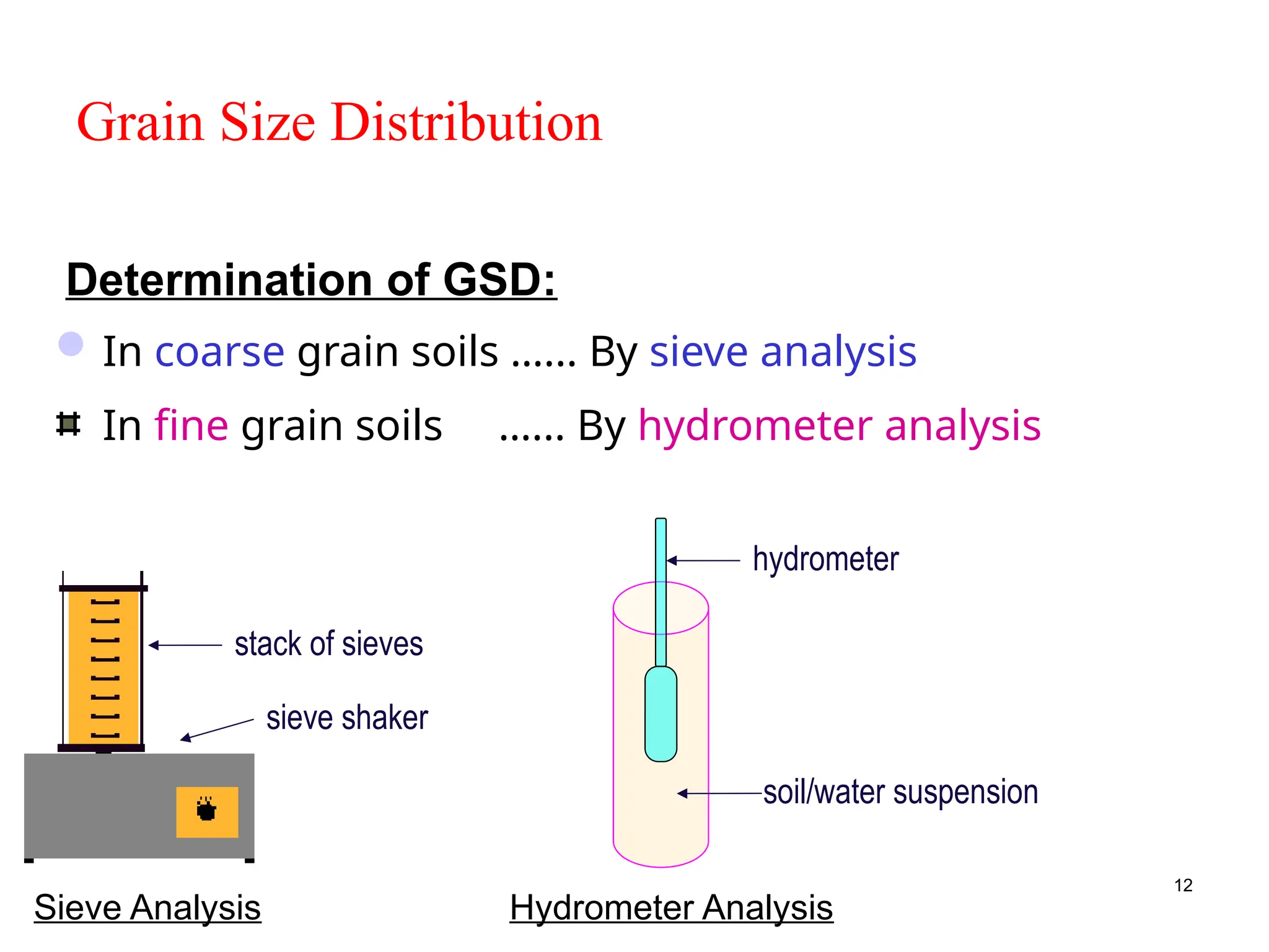
Grain Size Distribution
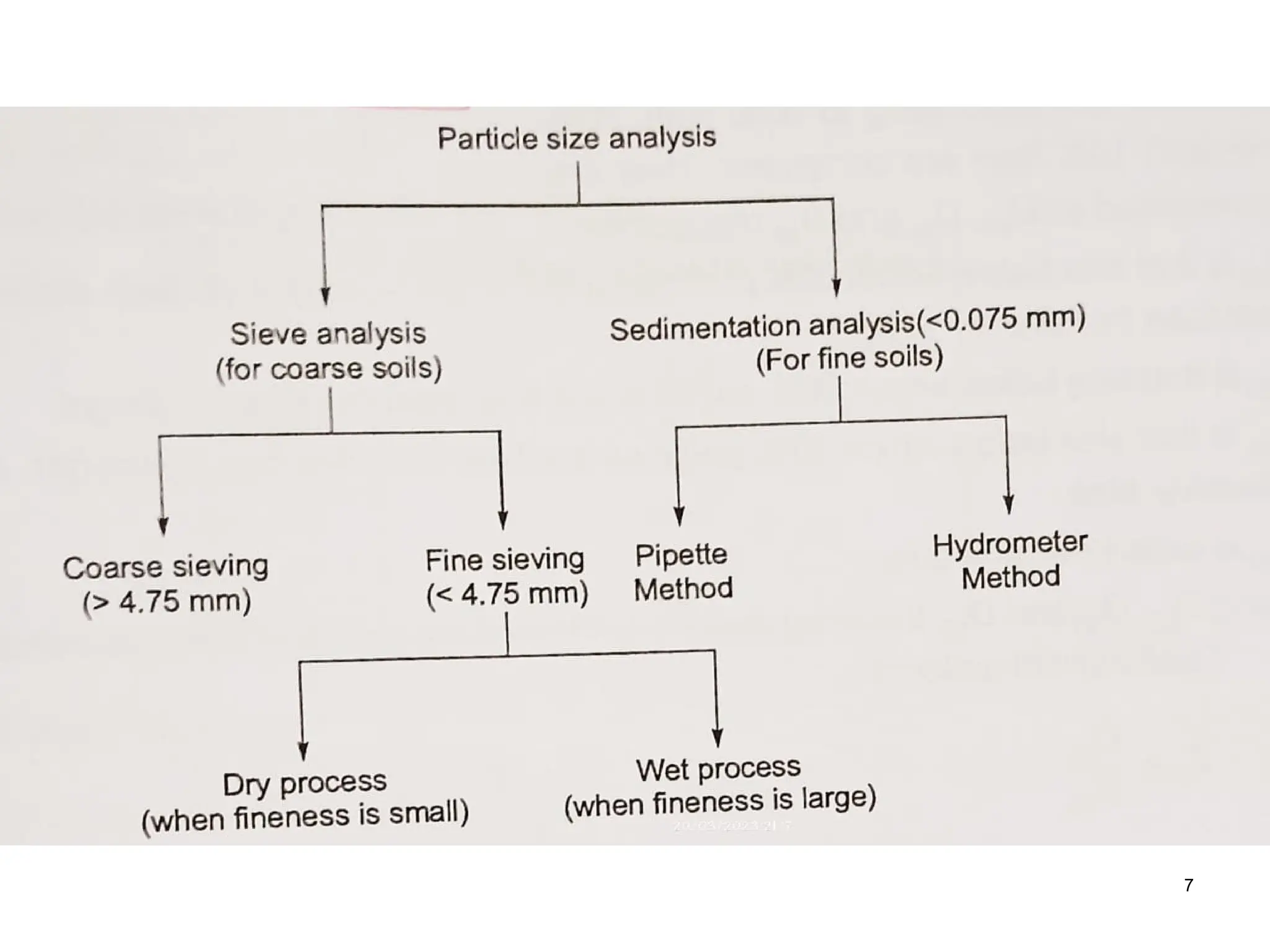
In coarse grain soils …... By sieve analysis
Determination of GSD:
In fine grain soils …... By hydrometer analysis
Sieve Analysis Hydrometer Analysis
soil/water suspension
hydrometer
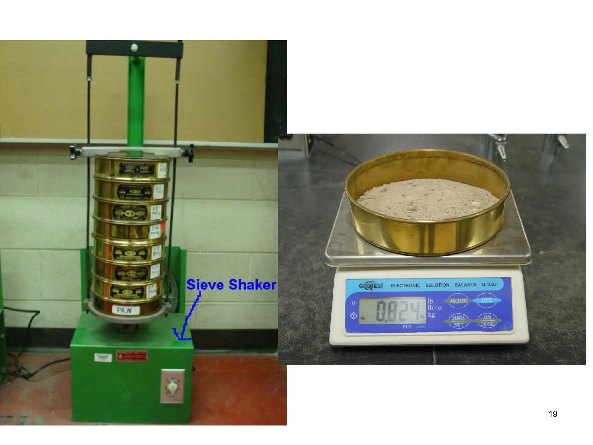
stack of sieves
sieve shaker

14
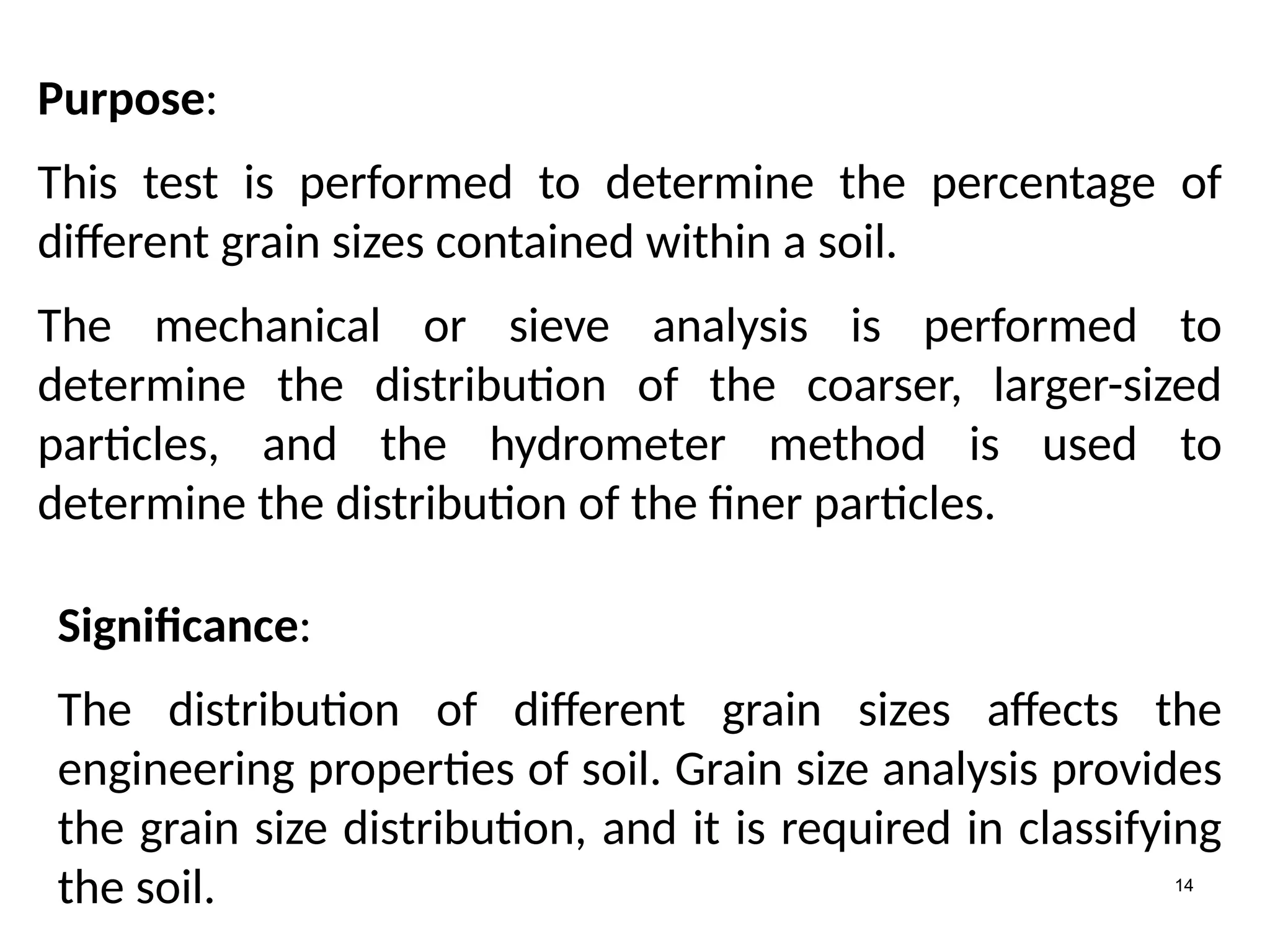
Purpose:
This test is performed to determine the percentage of
different grain sizes contained within a soil.
The mechanical or sieve analysis is performed to
determine the distribution of the coarser, larger-sized
particles, and the hydrometer method is used to
determine the distribution of the finer particles.
Significance:
The distribution of different grain sizes affects the
engineering properties of soil. Grain size analysis provides
the grain size distribution, and it is required in classifying
the soil.

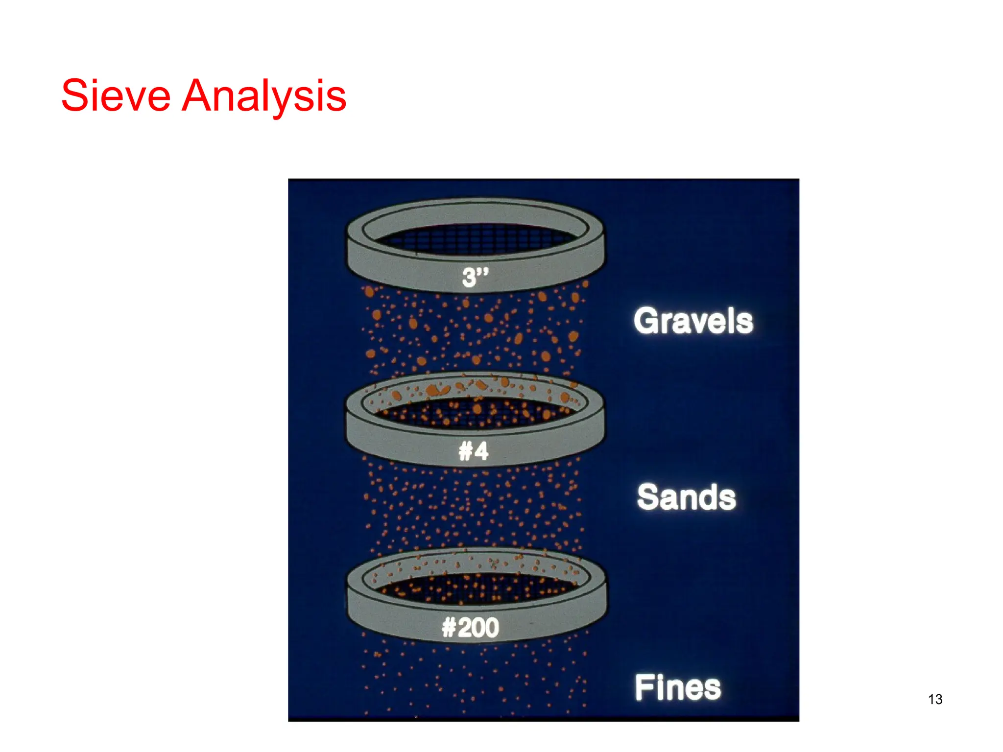
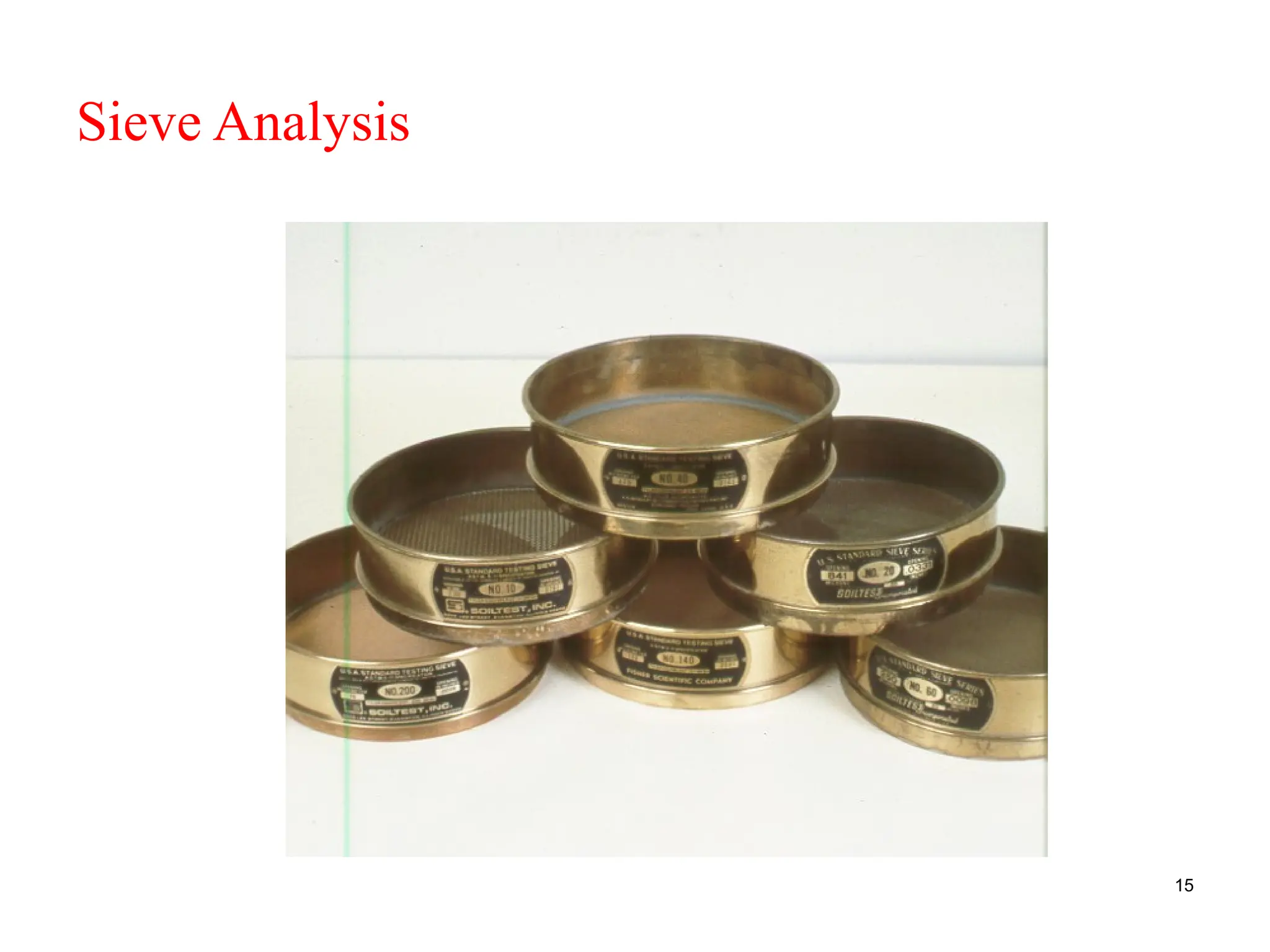
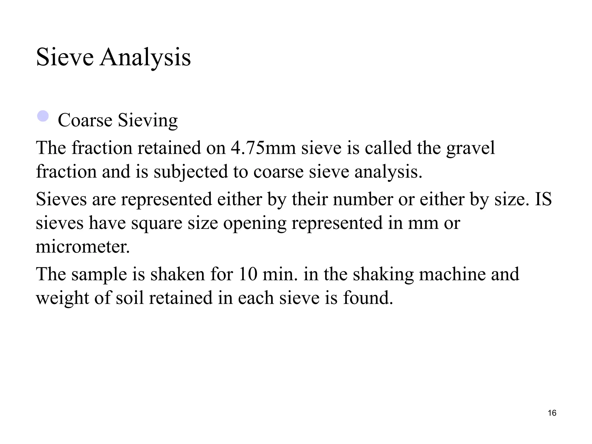
Sieve Analysis
Coarse Sieving
The fraction retained on 4.75mm sieve is called the gravel
fraction and is subjected to coarse sieve analysis.
Sieves are represented either by their number or either by size. IS
sieves have square size opening represented in mm or
micrometer.
The sample is shaken for 10 min. in the shaking machine and
weight of soil retained in each sieve is found.
16

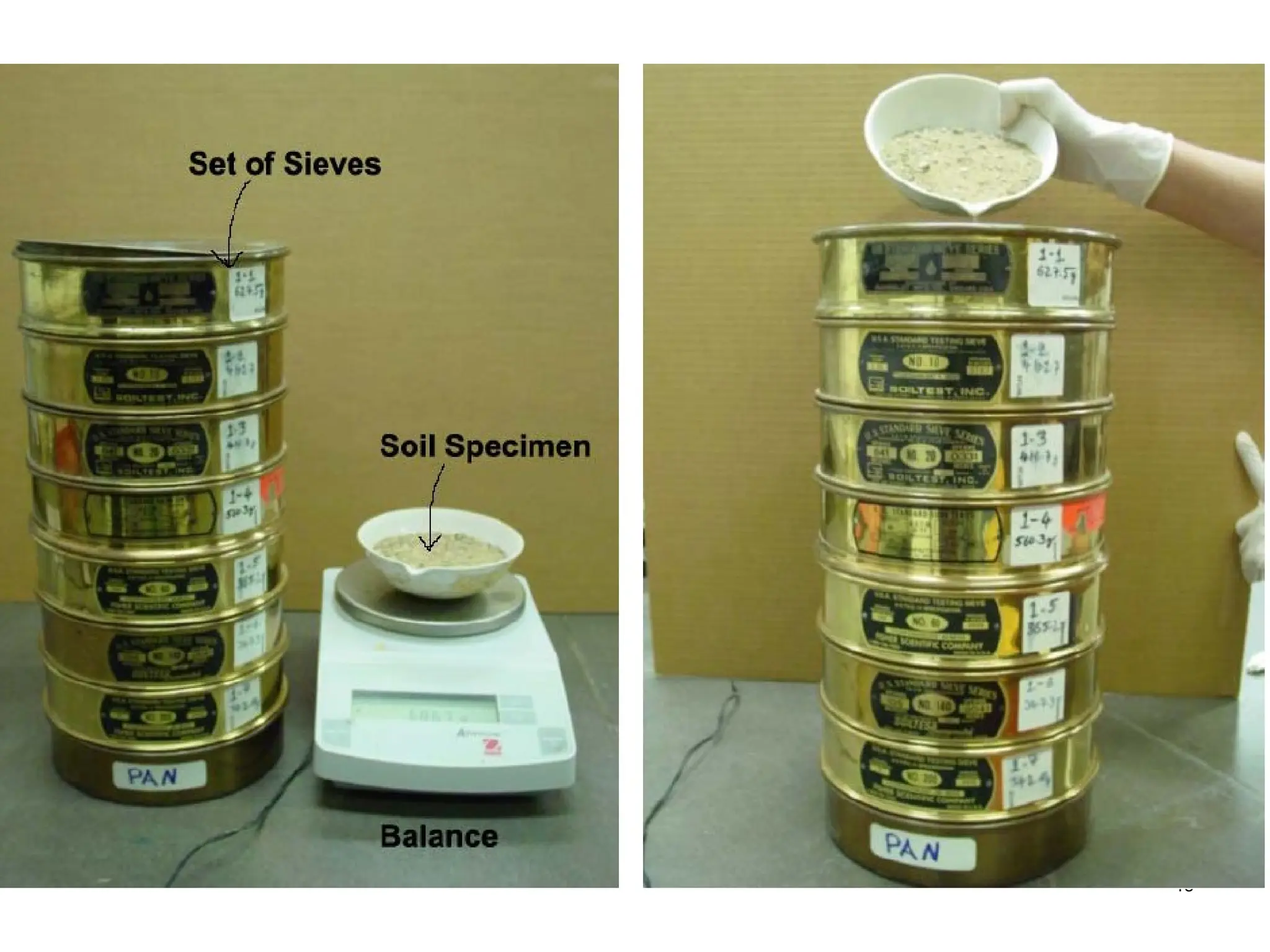
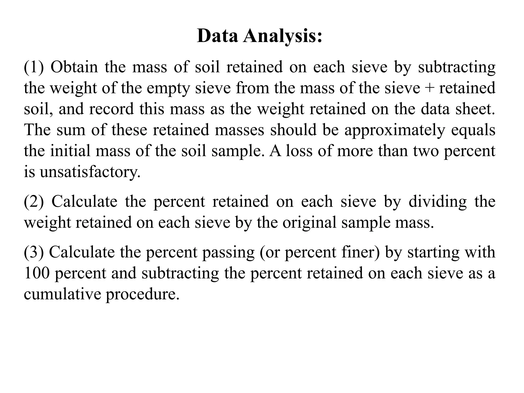
Data Analysis:
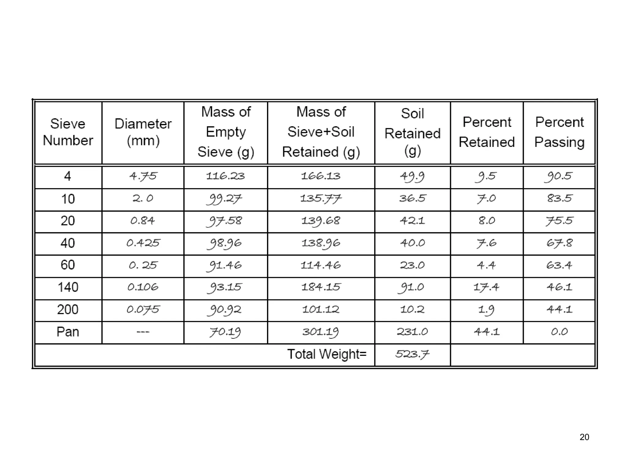
(1) Obtain the mass of soil retained on each sieve by subtracting
the weight of the empty sieve from the mass of the sieve + retained
soil, and record this mass as the weight retained on the data sheet.
The sum of these retained masses should be approximately equals
the initial mass of the soil sample. A loss of more than two percent
is unsatisfactory.
(2) Calculate the percent retained on each sieve by dividing the
weight retained on each sieve by the original sample mass.
(3) Calculate the percent passing (or percent finer) by starting with
100 percent and subtracting the percent retained on each sieve as a
cumulative procedure.

22
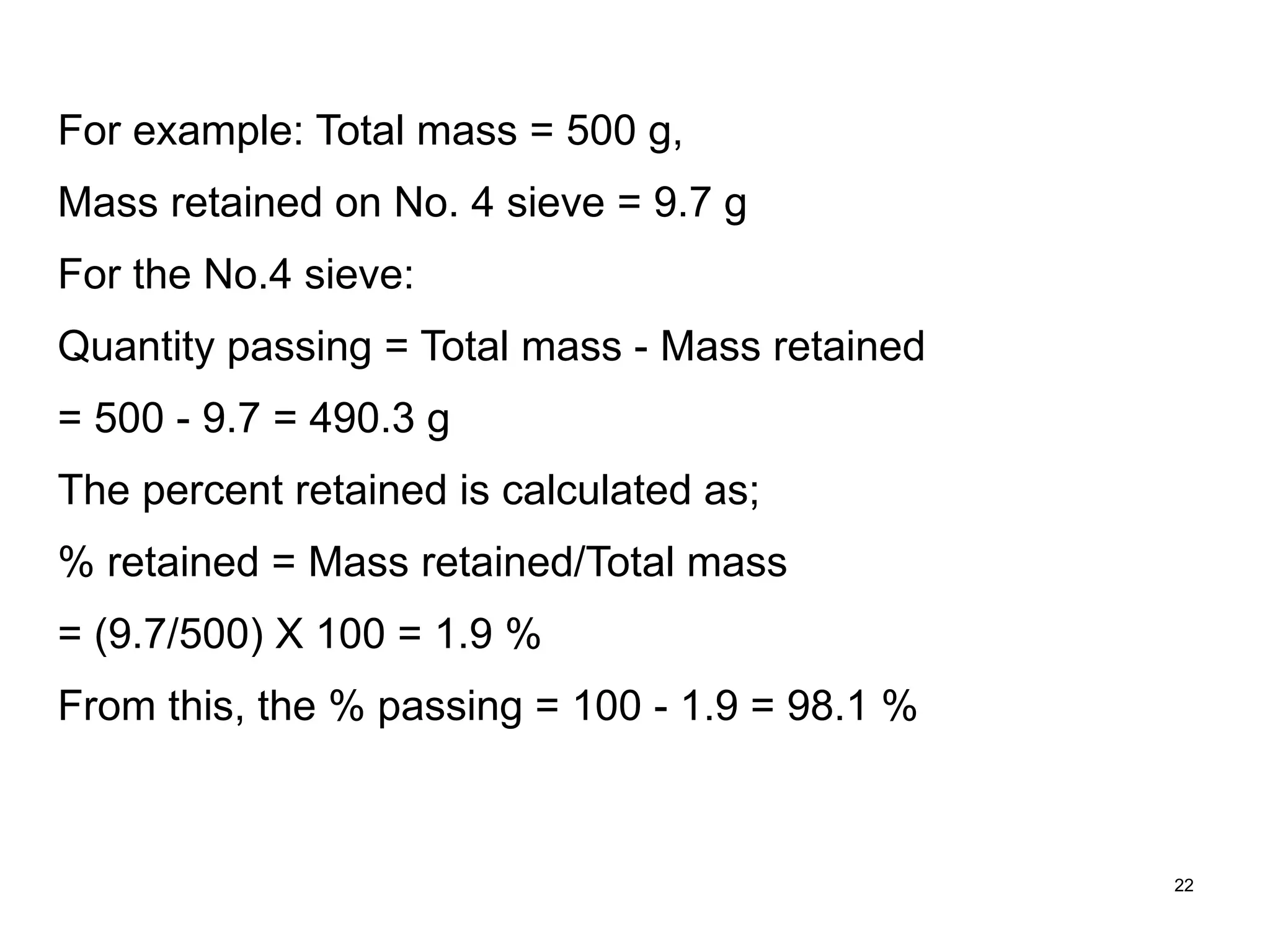
For example: Total mass = 500 g,
Mass retained on No. 4 sieve = 9.7 g
For the No.4 sieve:
Quantity passing = Total mass - Mass retained
= 500 - 9.7 = 490.3 g
The percent retained is calculated as;
% retained = Mass retained/Total mass
= (9.7/500) X 100 = 1.9 %
From this, the % passing = 100 - 1.9 = 98.1 %

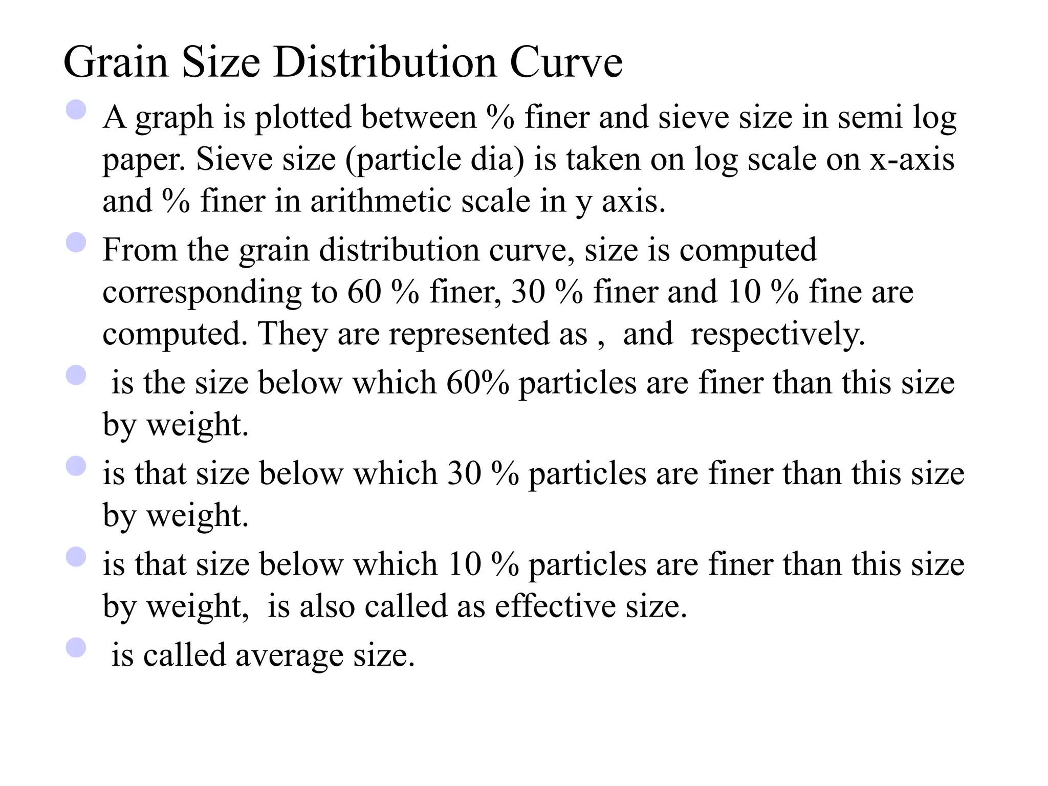
Grain Size Distribution Curve
A graph is plotted between % finer and sieve size in semi log
paper. Sieve size (particle dia) is taken on log scale on x-axis
and % finer in arithmetic scale in y axis.
From the grain distribution curve, size is computed
corresponding to 60 % finer, 30 % finer and 10 % fine are
computed. They are represented as , and respectively.
 is the size below which 60% particles are finer than this size
by weight.
is that size below which 30 % particles are finer than this size
by weight.
is that size below which 10 % particles are finer than this size
by weight, is also called as effective size.
 is called average size.

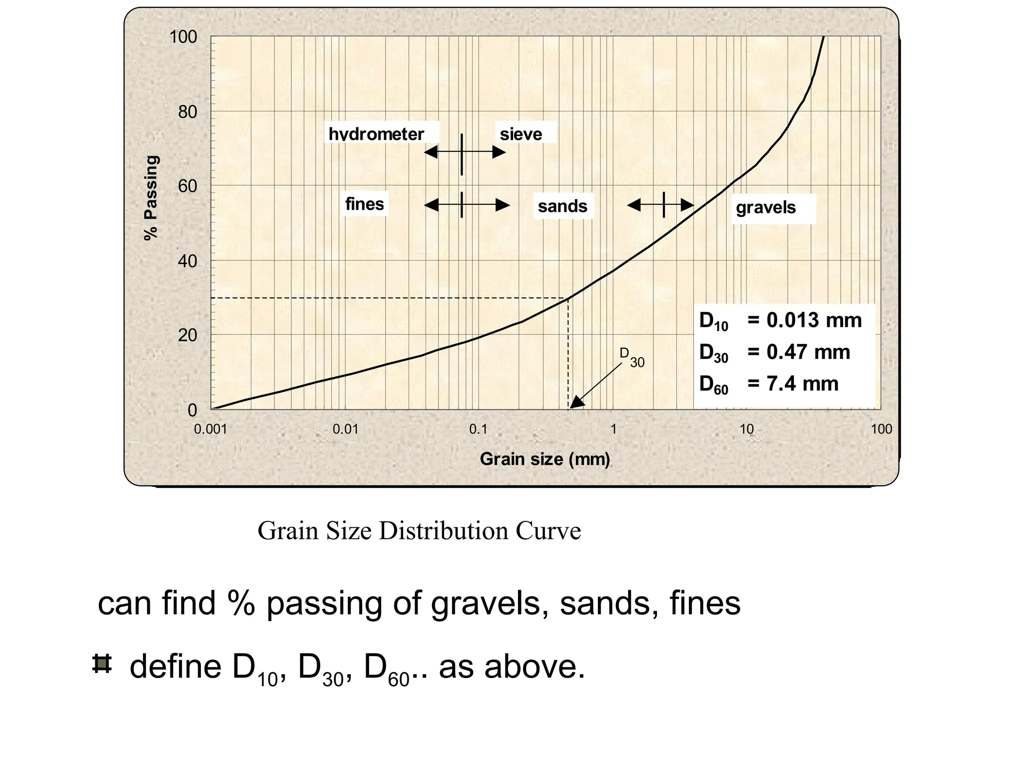
Grain Size Distribution Curve
can find % passing of gravels, sands, fines
define D10, D30, D60.. as above.
0
20
40
60
80
100
0.001 0.01 0.1 1 10 100
Grain size (mm)
D
30
sieve
hydrometer
D10 = 0.013 mm
D30 = 0.47 mm
D60 = 7.4 mm
sands gravels
fines
%
Passing

25
Grading curves
0.0001 0.001 0.01 0.1 1 10 100
0
20
40
60
80
100
Particle size (mm)
%
F
ine
r
W Well graded

26
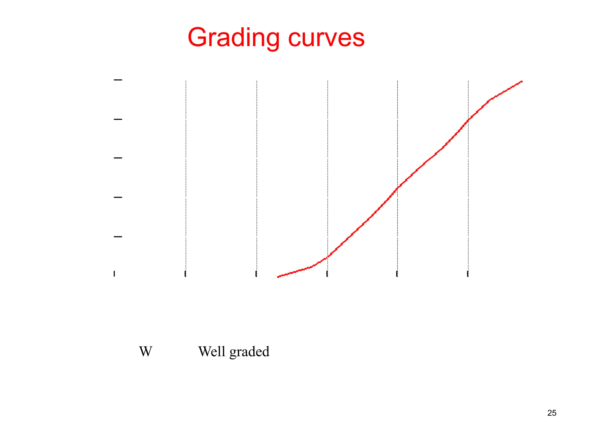
Grading curves
0.0001 0.001 0.01 0.1 1 10 100
0
20
40
60
80
100
Particle size (mm)
%
F
ine
r
W Well graded
U Uniformly graded

27
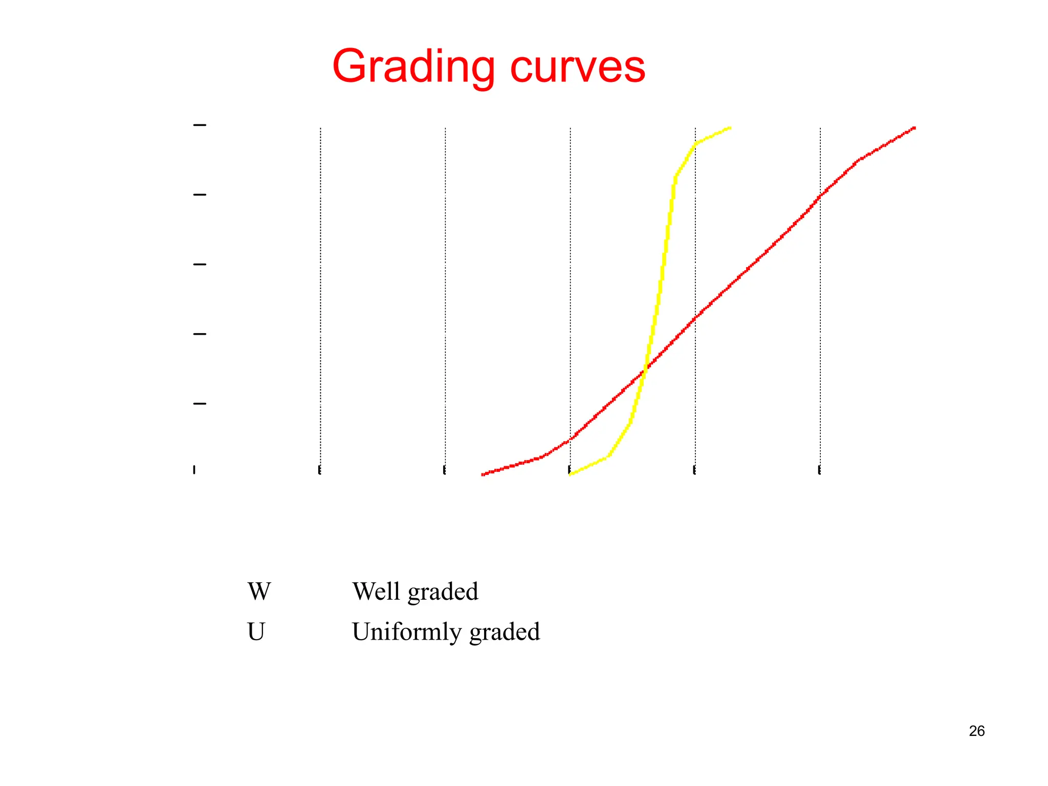
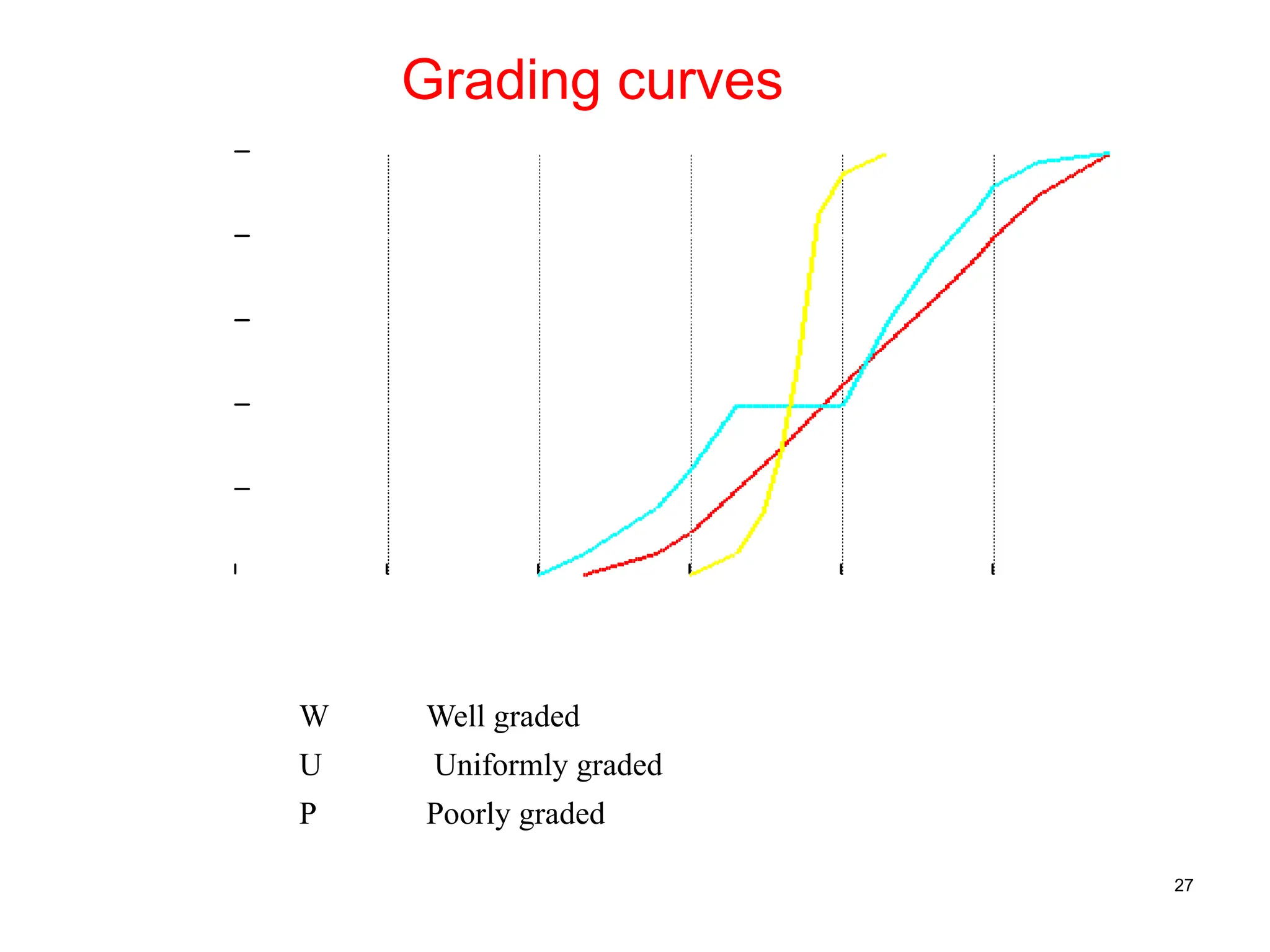
Grading curves
0.0001 0.001 0.01 0.1 1 10 100
0
20
40
60
80
100
Particle size (mm)
%
F
ine
r
W Well graded
U Uniformly graded
P Poorly graded

28
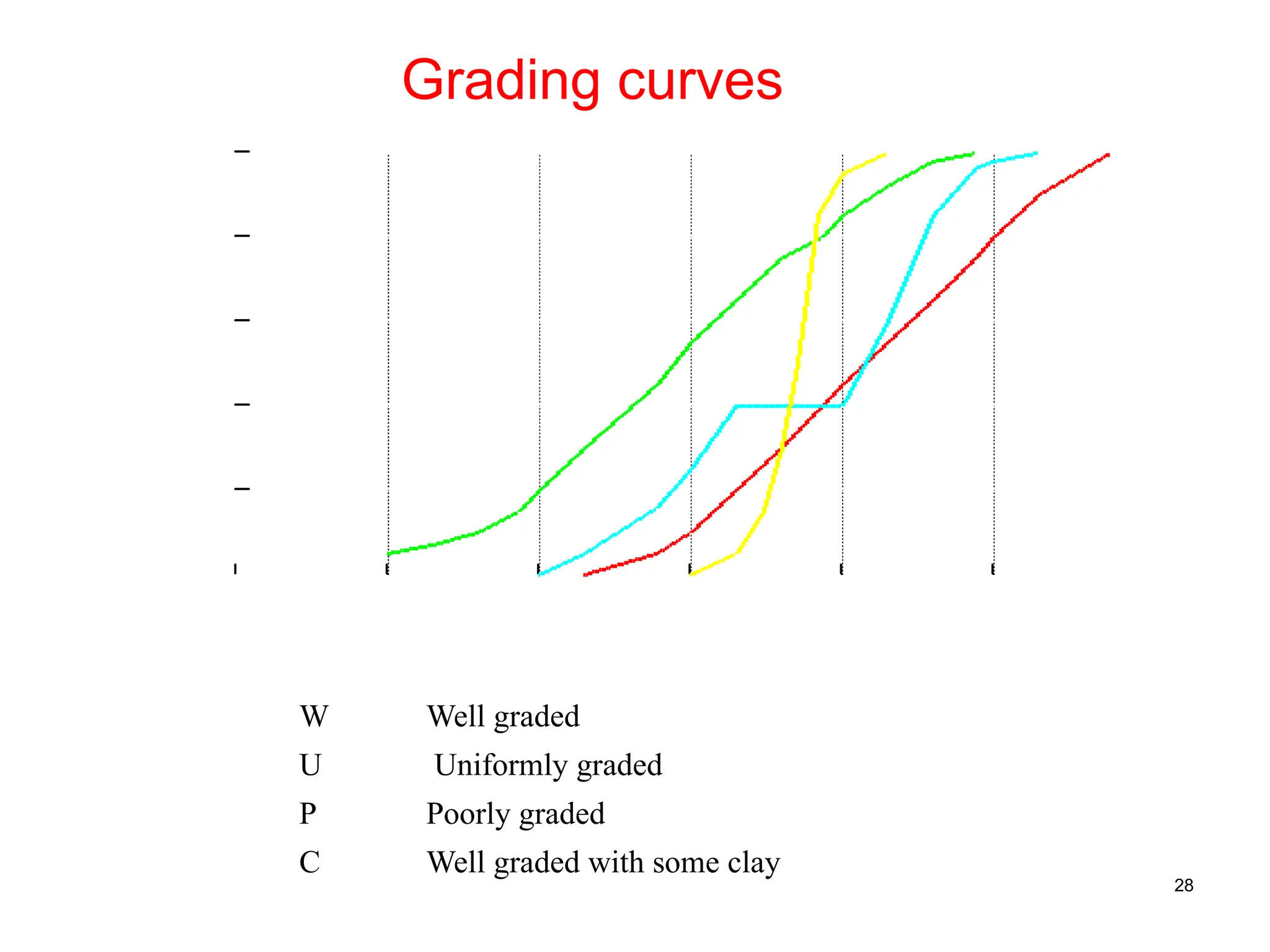
Grading curves
0.0001 0.001 0.01 0.1 1 10 100
0
20
40
60
80
100
Particle size (mm)
%
F
ine
r
W Well graded
U Uniformly graded
P Poorly graded
C Well graded with some clay

29
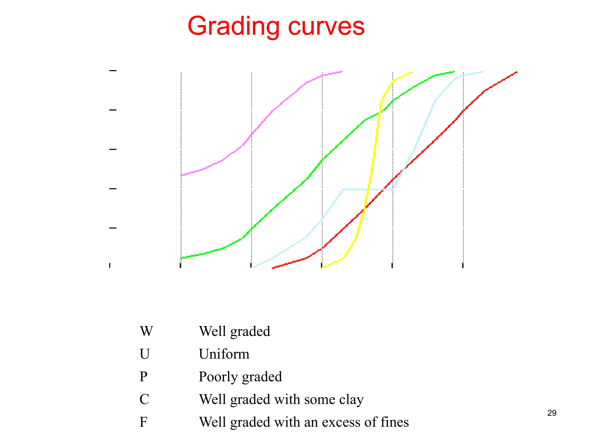
Grading curves
0.0001 0.001 0.01 0.1 1 10 100
0
20
40
60
80
100
Particle size (mm)
%
F
ine
r
W Well graded
U Uniform
P Poorly graded
C Well graded with some clay
F Well graded with an excess of fines

30
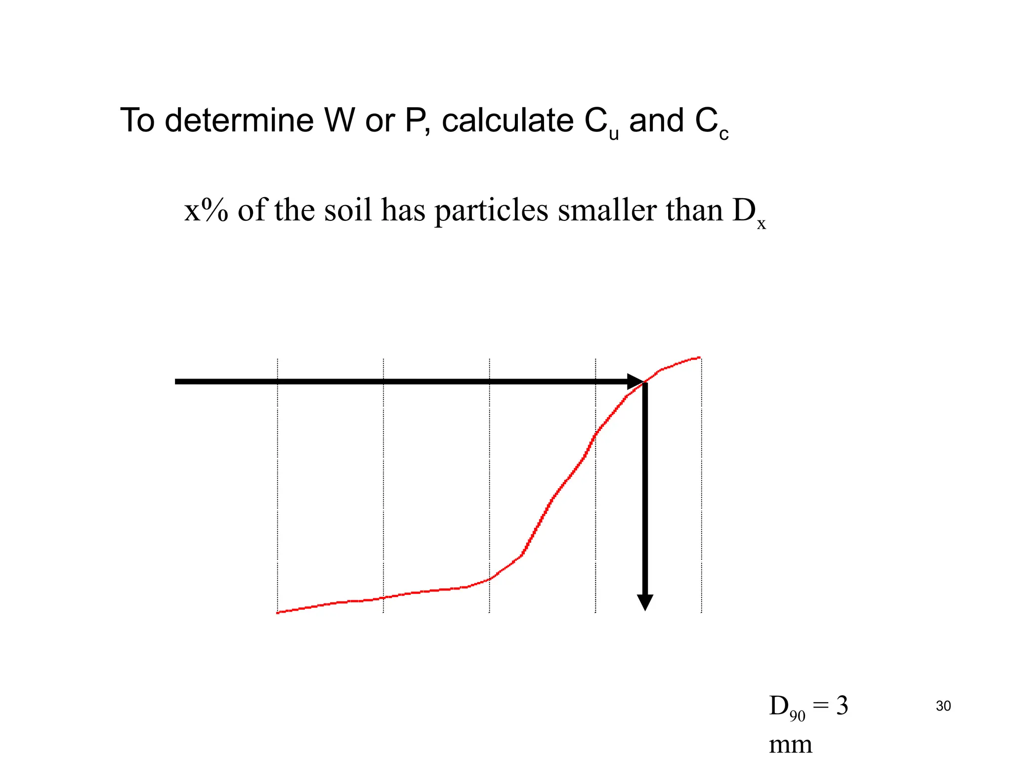
To determine W or P, calculate Cu and Cc
0.0001 0.001 0.01 0.1 1 10 100
0
20
40
60
80
100
Particle size (mm)
%
F
i
n
e
r
D90 = 3
mm
x% of the soil has particles smaller than Dx

31
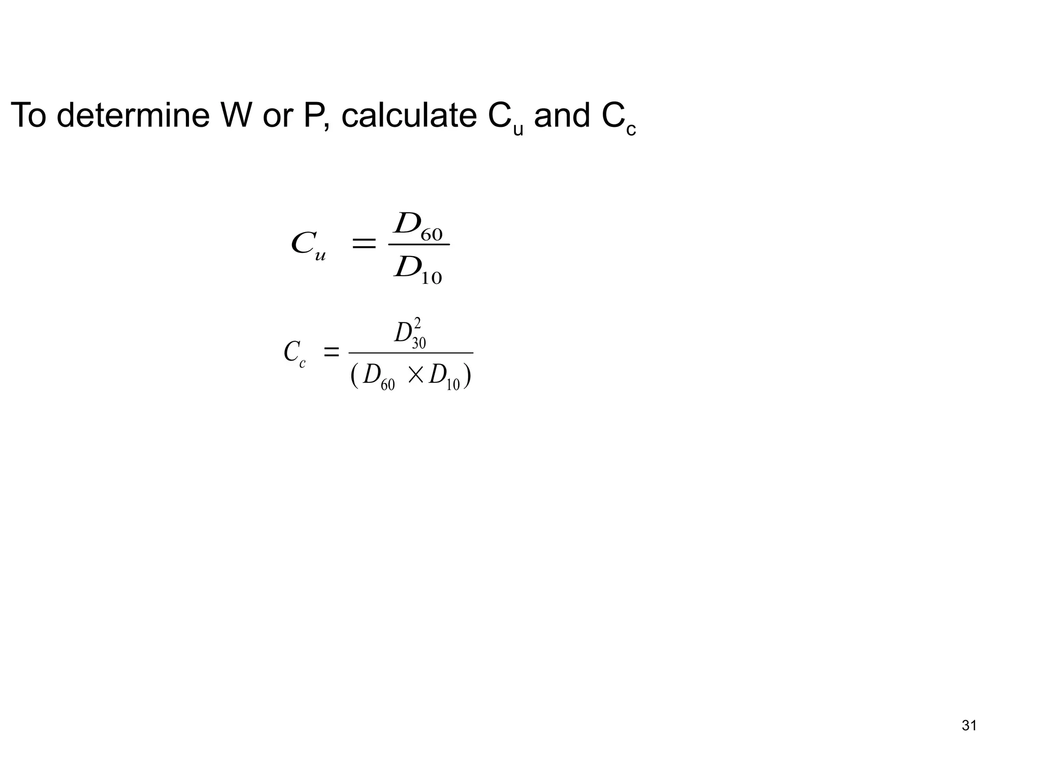
To determine W or P, calculate Cu and Cc
C
D
D
u  60
10
C
D
D D
c 

30
2
60 10
( )

32
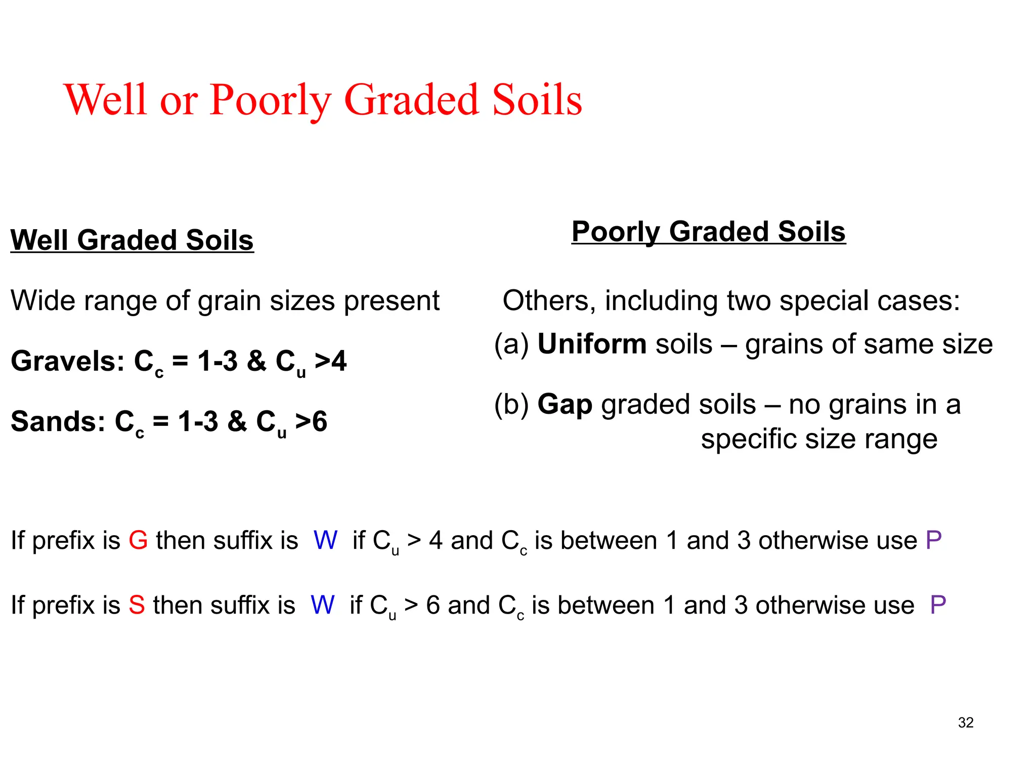
Well or Poorly Graded Soils
Well Graded Soils Poorly Graded Soils
Wide range of grain sizes present
Gravels: Cc = 1-3 & Cu >4
Sands: Cc = 1-3 & Cu >6
Others, including two special cases:
(a) Uniform soils – grains of same size
(b) Gap graded soils – no grains in a
specific size range
If prefix is G then suffix is W if Cu > 4 and Cc is between 1 and 3 otherwise use P
If prefix is S then suffix is W if Cu > 6 and Cc is between 1 and 3 otherwise use P

Relative density and consistency of
soil
33

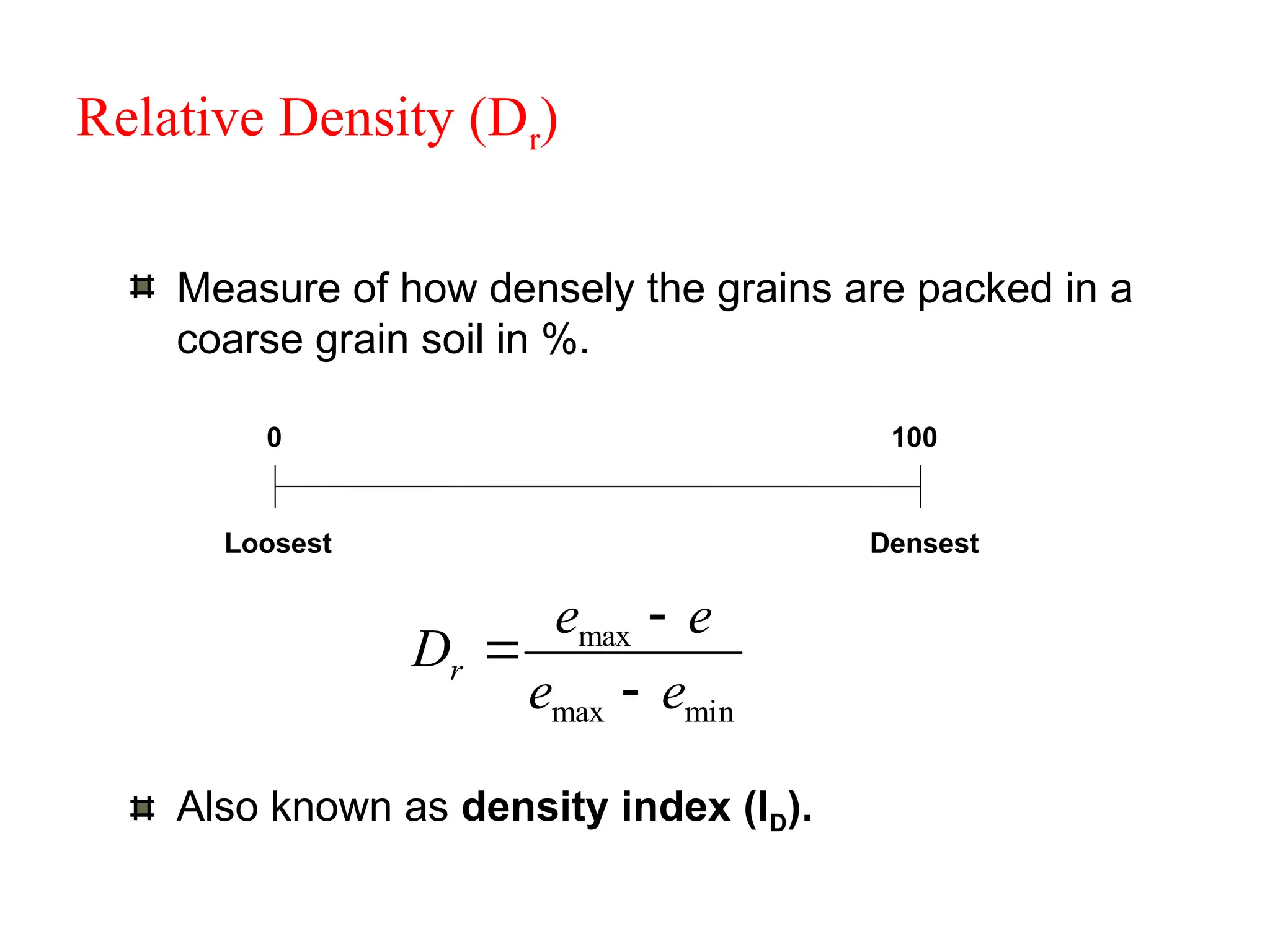
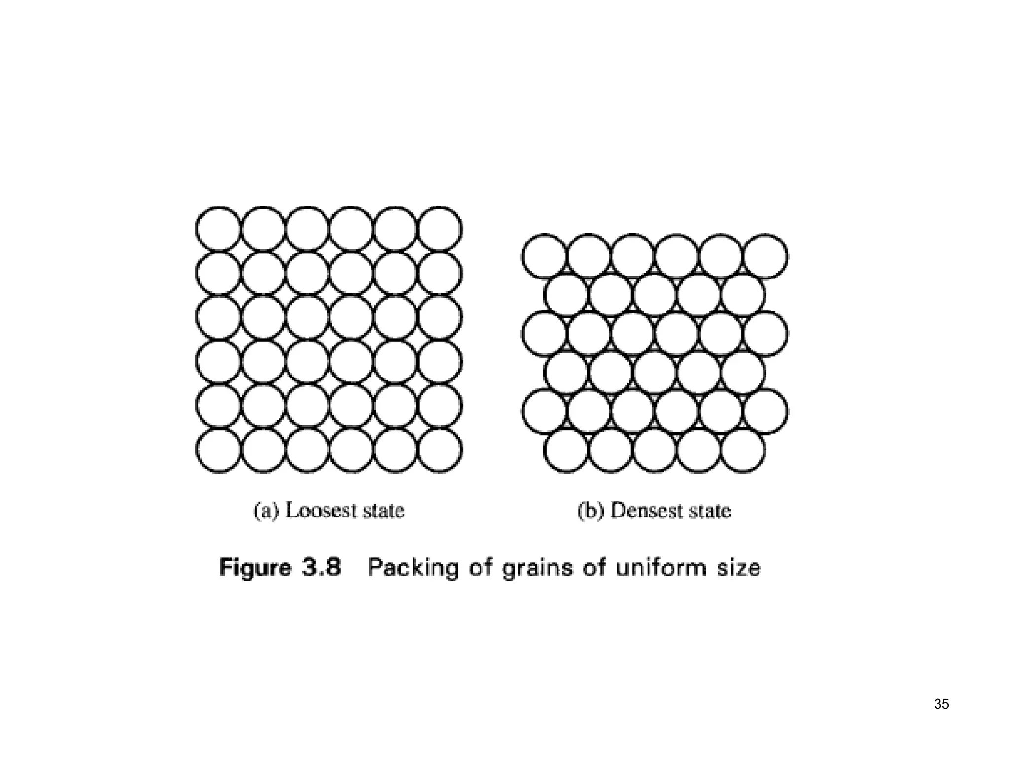
Relative Density (Dr)
Measure of how densely the grains are packed in a
coarse grain soil in %.
0 100
Loosest Densest
min
max
max
e
e
e
e
Dr



Also known as density index (ID).

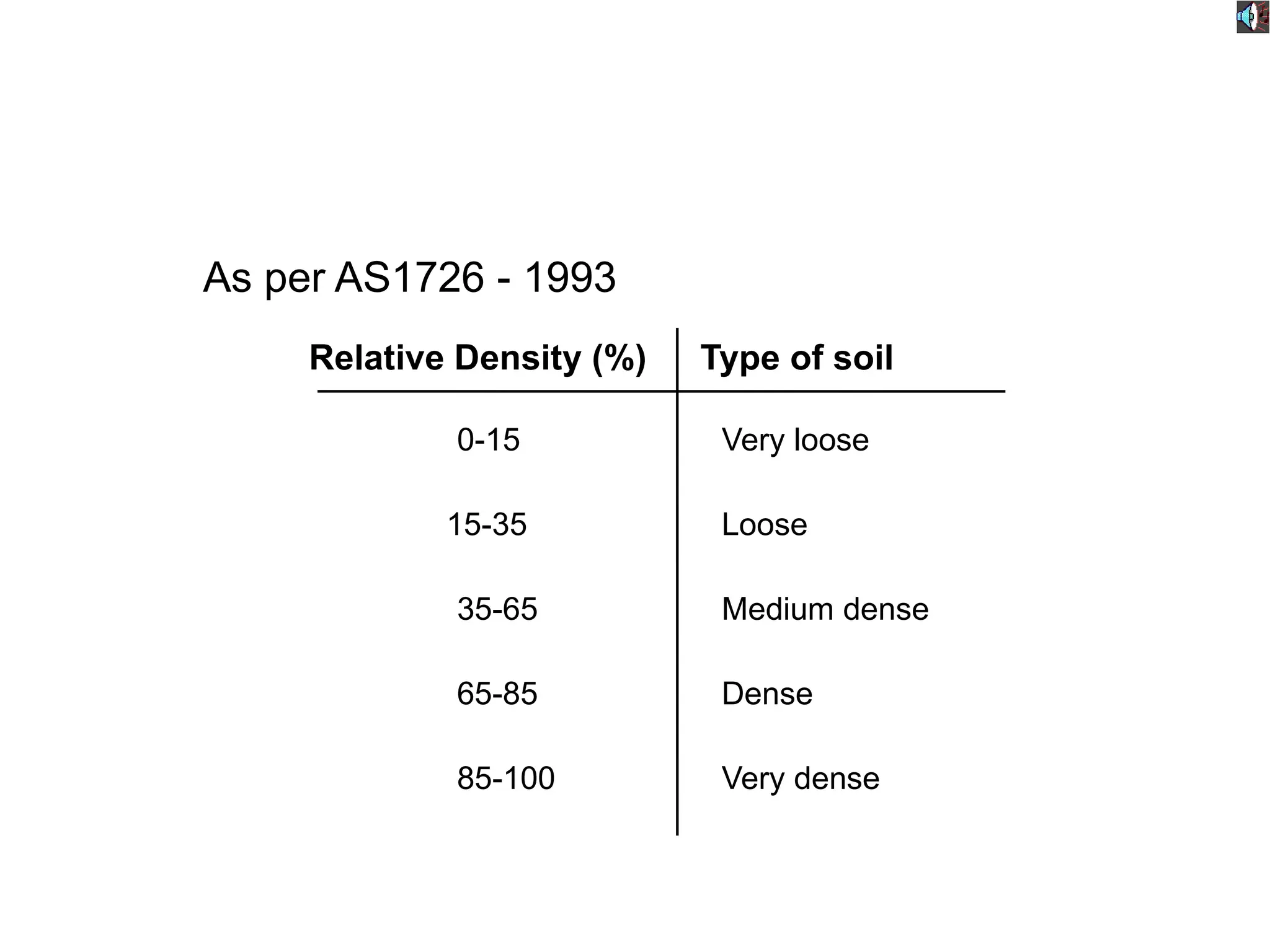
As per AS1726 - 1993
Relative Density (%) Type of soil
0-15
15-35
35-65
65-85
85-100
Very loose
Loose
Medium dense
Dense
Very dense

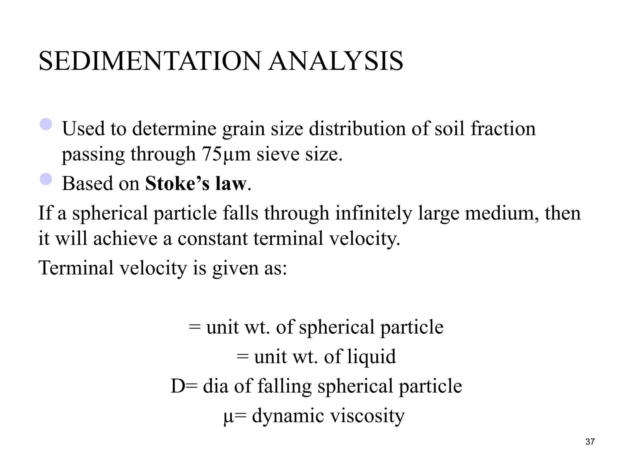
SEDIMENTATION ANALYSIS
Used to determine grain size distribution of soil fraction
passing through 75µm sieve size.
Based on Stoke’s law.
If a spherical particle falls through infinitely large medium, then
it will achieve a constant terminal velocity.
Terminal velocity is given as:
= unit wt. of spherical particle
= unit wt. of liquid
D= dia of falling spherical particle
µ= dynamic viscosity
37

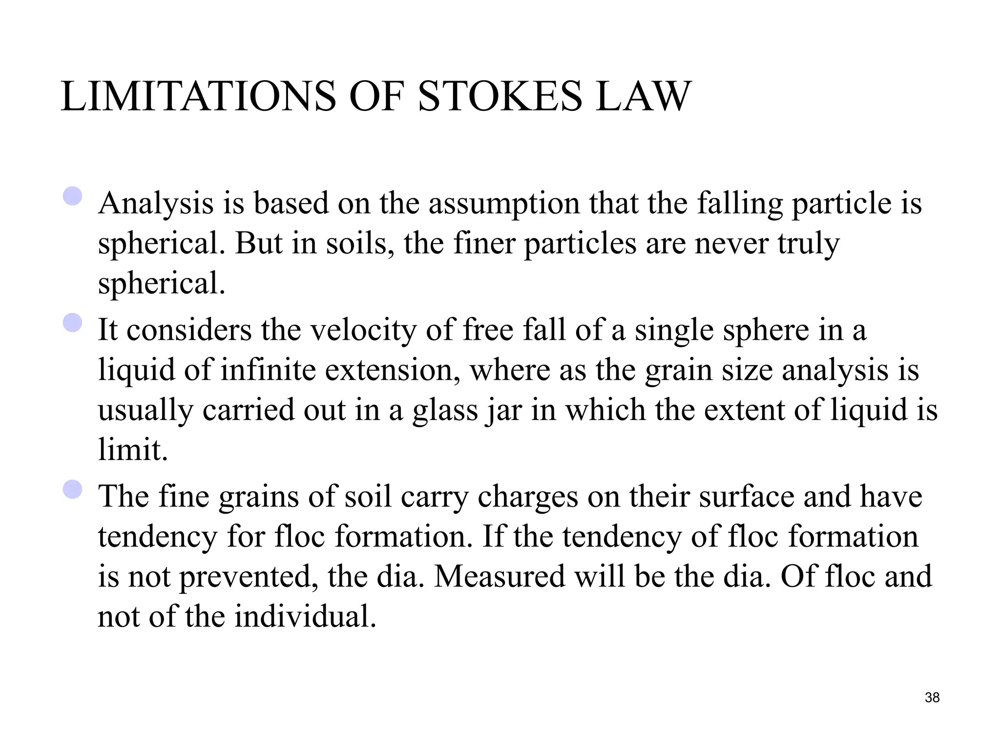
LIMITATIONS OF STOKES LAW
Analysis is based on the assumption that the falling particle is
spherical. But in soils, the finer particles are never truly
spherical.
It considers the velocity of free fall of a single sphere in a
liquid of infinite extension, where as the grain size analysis is
usually carried out in a glass jar in which the extent of liquid is
limit.
The fine grains of soil carry charges on their surface and have
tendency for floc formation. If the tendency of floc formation
is not prevented, the dia. Measured will be the dia. Of floc and
not of the individual.
38

Procedure of Sedimentation Analysis:
First step involved is the preparation of soil sample. Soil sample
is mixed with water and suspension is made.
Treatment given to soil sample:
Pre-treatment: Treatment given before making soil
suspension to remove organic matter and calcium compounds.
For organic matter- Oxidizing Agent is used
For Calcium Compounds – Acids are used (HCl)
Post-treatment: done after preparation of soil suspension to
break flocs that are formed due to presence of surface electric
charges. Deflocculating Agents used are : Sodium hexameta
phosphate, Sodium Oxalate etc.
39

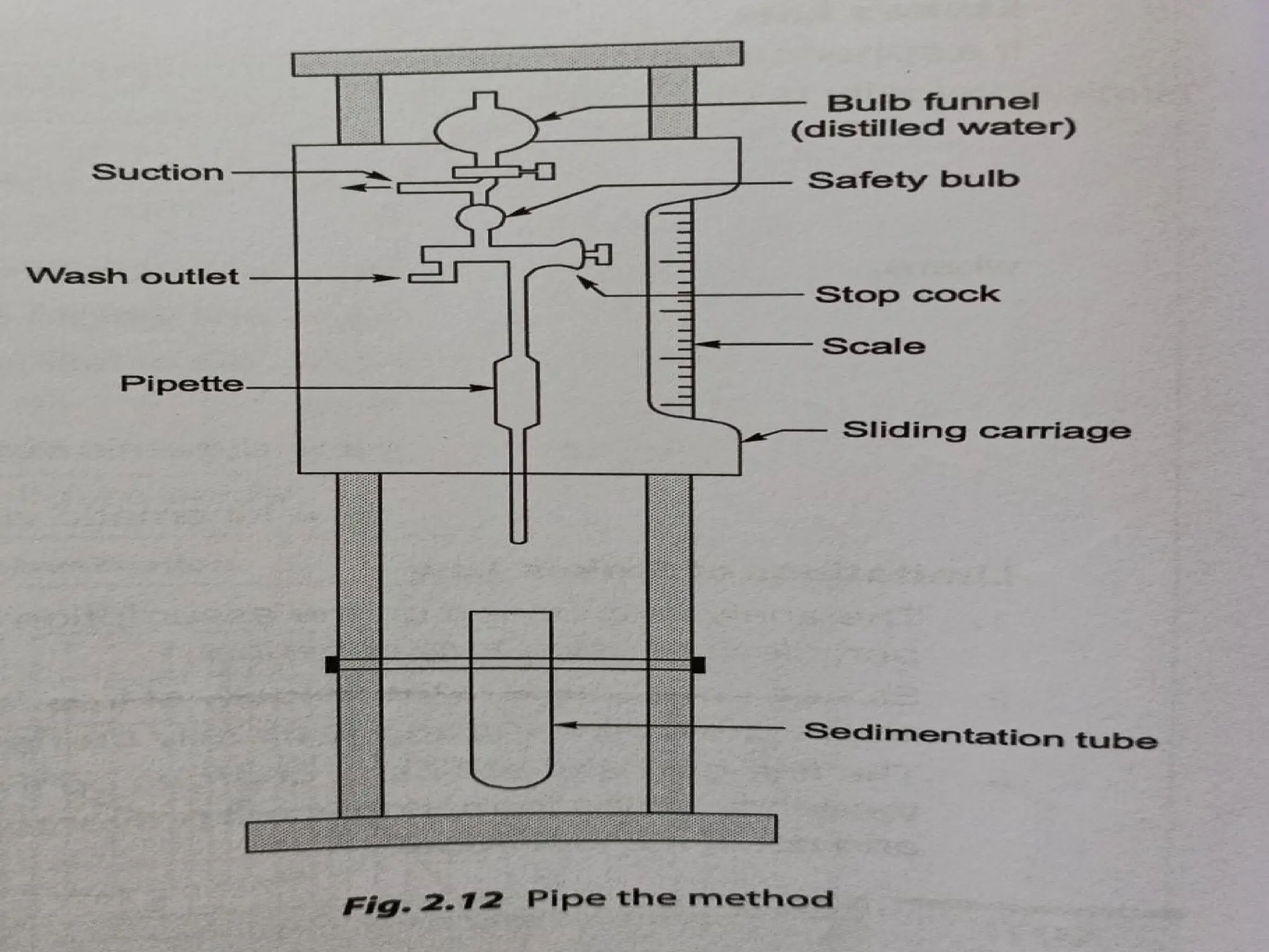
The analysis is carried out by the hydrometer or pipette method.
The principle of the test is same in both methods. The difference
lies only in the method of making the observations.
40

Pipette Method:
Let M= total mass of dry soil which is used to prepare
suspension having total volume V.
10ml sample of suspension is drawn off with a pipette from a
specified depth from the surface at different time intervals.
This 10ml sample is put in a container and is dried in oven to
get dry unit weight/dry density.
Let = mass of dried sample obtained from pipette
Volume(=10ml)
Hence, mass per unit volume of dried sample
41

If dispersing agent as added in the total Volume V, of mass.
Then mass per unit vol. of dispersing agent
The mass per unit Vol. of soil solids at any time interval is
given by
Percentage finer is given by
The dia. Of filling particle at any instance of time is given by the Stokes
Law
= effective depth through which particle settles
42

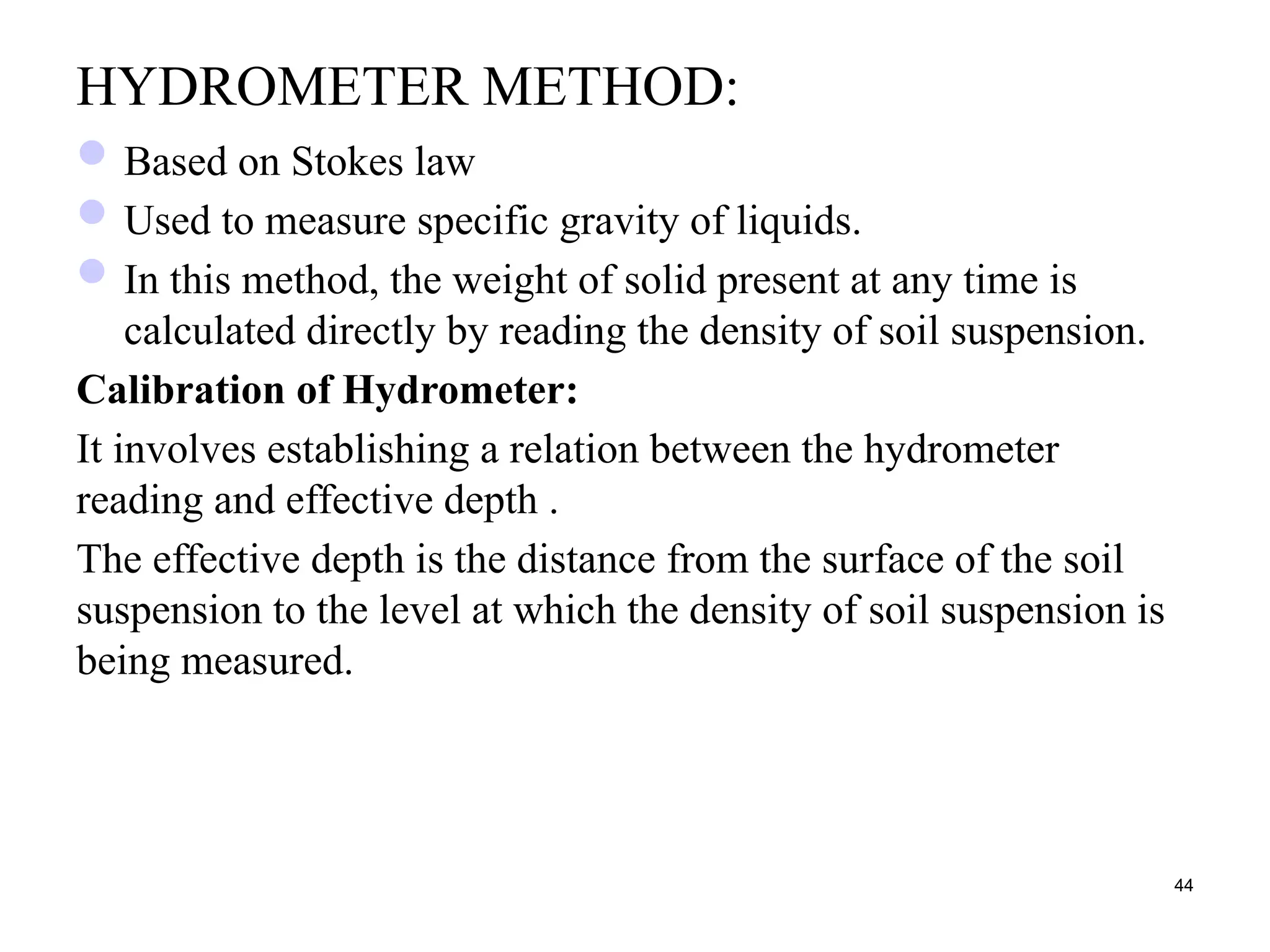
HYDROMETER METHOD:
Based on Stokes law
Used to measure specific gravity of liquids.
In this method, the weight of solid present at any time is
calculated directly by reading the density of soil suspension.
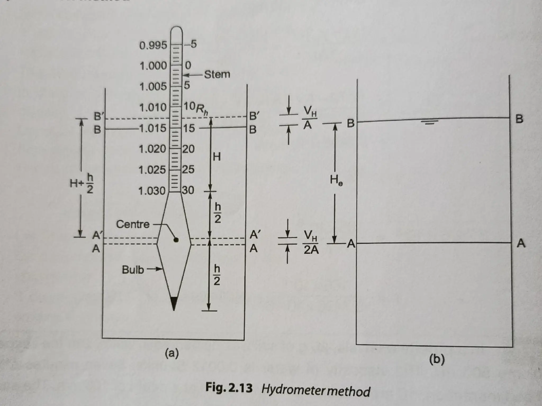
Calibration of Hydrometer:
It involves establishing a relation between the hydrometer
reading and effective depth .
The effective depth is the distance from the surface of the soil
suspension to the level at which the density of soil suspension is
being measured.
44

Effective depth
= distance (cm) between any hydrometer reading and
neck
h= length of hydrometer bulb
= vol. of hydrometer bulb
= area of cross section of the jar
Reading of hydrometer is related to specific gravity or density of
soil suspension as:
Thus a reading of =25 means 1.025
Thus a reading of =-25 means 0.975
46

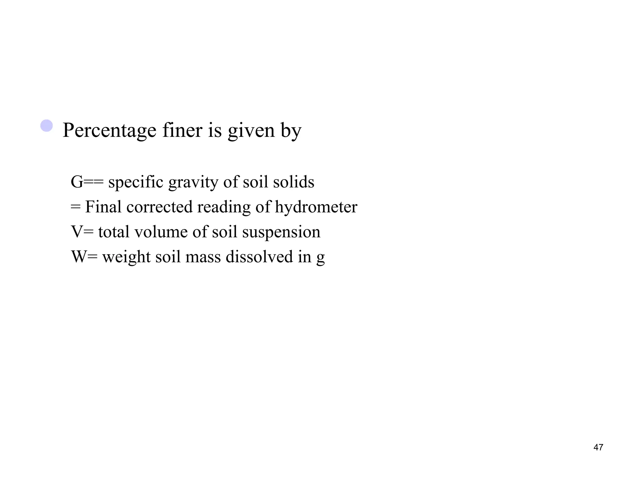
Percentage finer is given by
G== specific gravity of soil solids
= Final corrected reading of hydrometer
V= total volume of soil suspension
W= weight soil mass dissolved in g
47

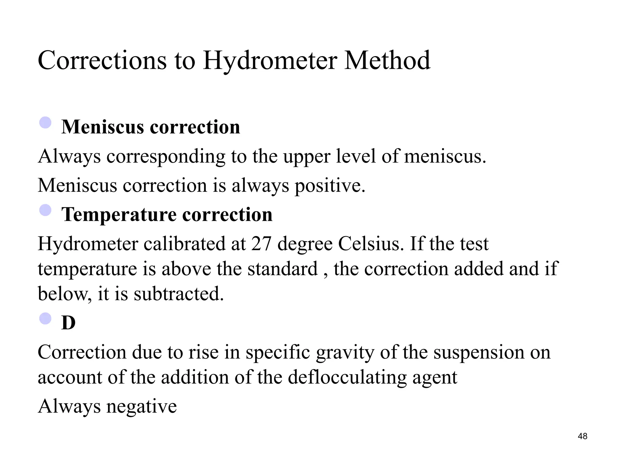
Corrections to Hydrometer Method
Meniscus correction
Always corresponding to the upper level of meniscus.
Meniscus correction is always positive.
Temperature correction
Hydrometer calibrated at 27 degree Celsius. If the test
temperature is above the standard , the correction added and if
below, it is subtracted.
D
Correction due to rise in specific gravity of the suspension on
account of the addition of the deflocculating agent
Always negative
48

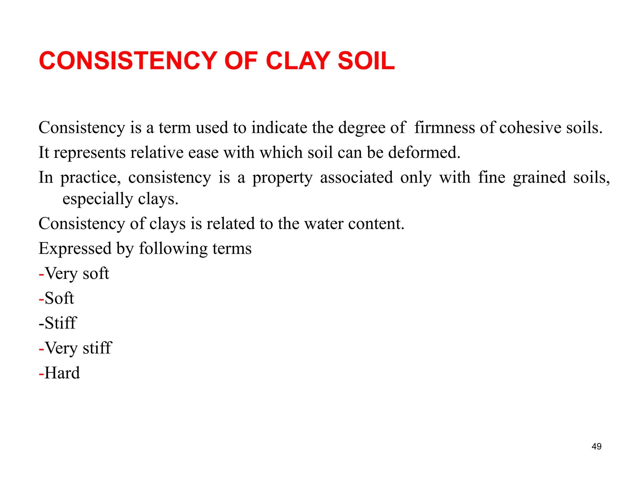
CONSISTENCY OF CLAY SOIL
Consistency is a term used to indicate the degree of firmness of cohesive soils.
It represents relative ease with which soil can be deformed.
In practice, consistency is a property associated only with fine grained soils,
especially clays.
Consistency of clays is related to the water content.
Expressed by following terms
-Very soft
-Soft
-Stiff
-Very stiff
-Hard
49

Consistency of a soil can be expressed in terms of:
1. Atterberg limits of soils (Liquid limit, Plastic limit, Shrinkage
limit)
2. Unconfined compressive strengths of soils.
50

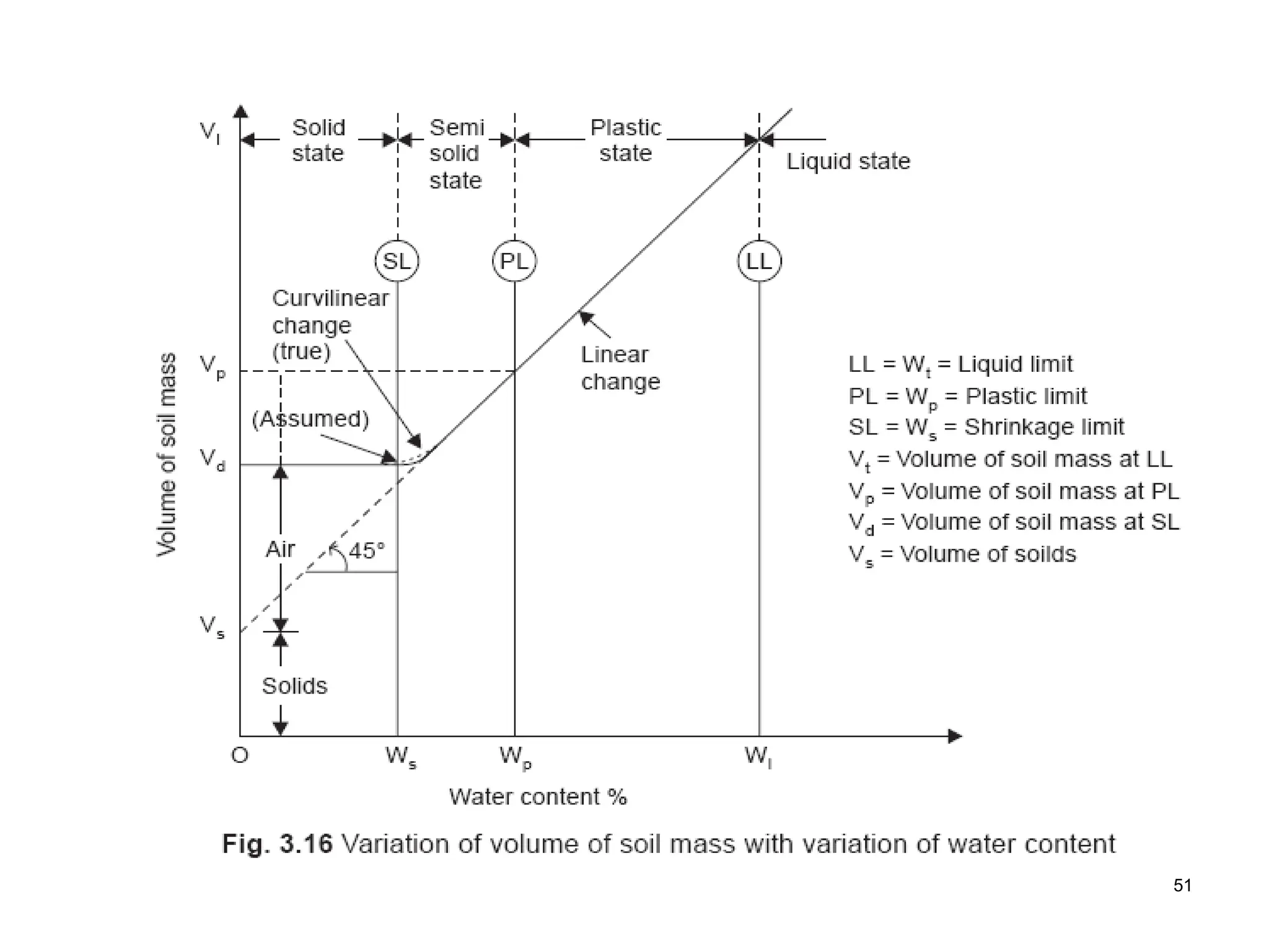
For change in water content corresponding to change degree
of saturation from 0% to 100%, there is no change in total
volume of soil. But for water content increasing greater than
shrinkage limit (S=100%), then with change in water content,
total volume of soil also changes.
At shrinkage limit all the pores of soil are just filled by water.
Hence degree of saturation (S) is 100%.
Naturally existing soils have water content between and
On increasing water content shear strength of soil decreases.
52

53
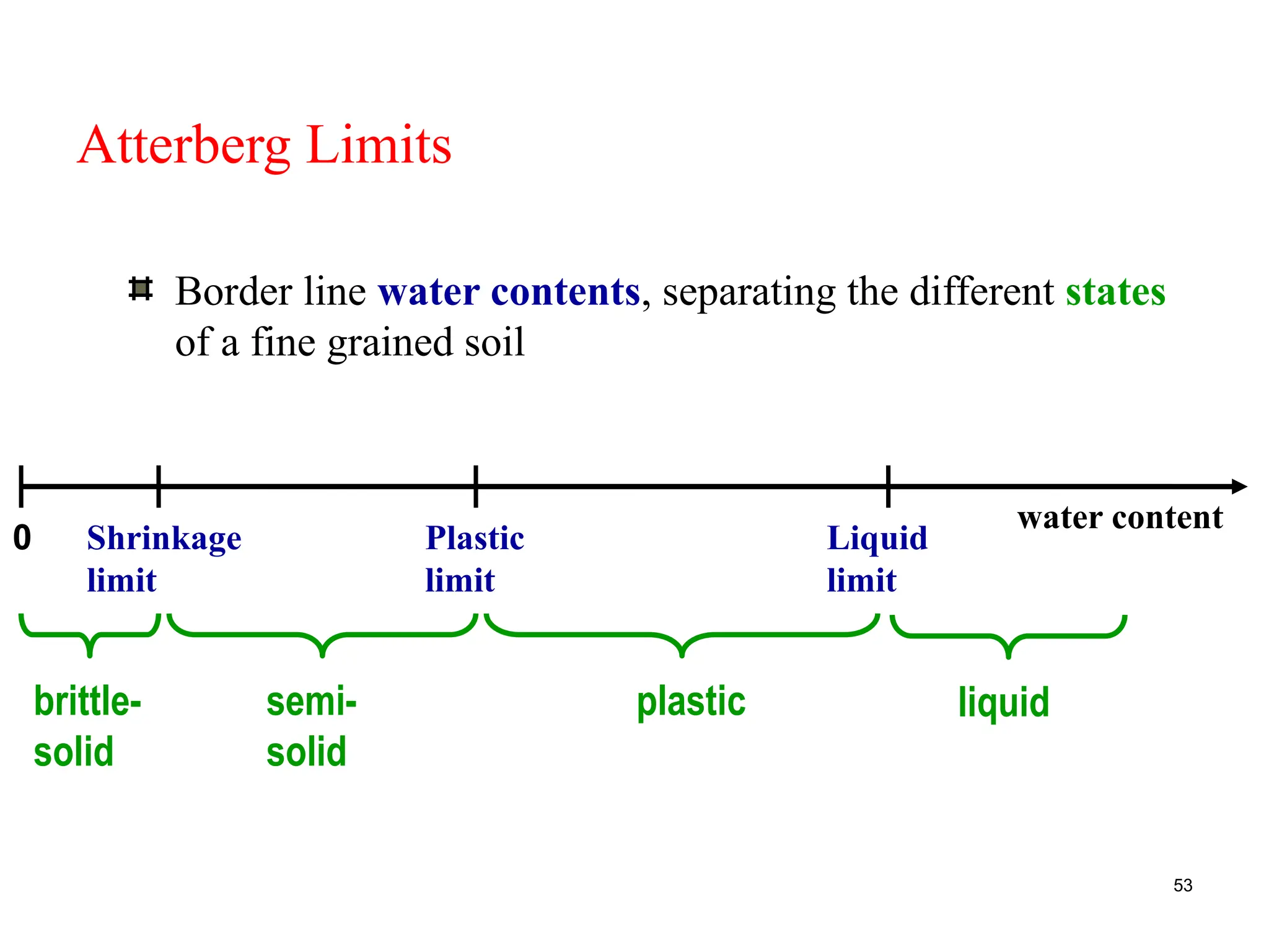
Atterberg Limits
Border line water contents, separating the different states
of a fine grained soil
Liquid
limit
Shrinkage
limit
Plastic
limit
0
water content
liquid
semi-
solid
brittle-
solid
plastic

54
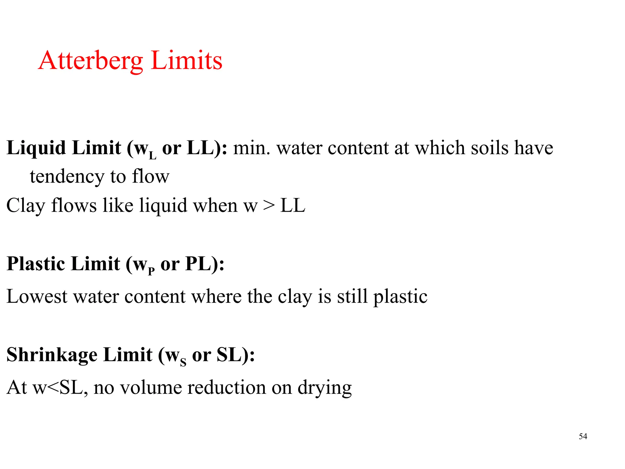
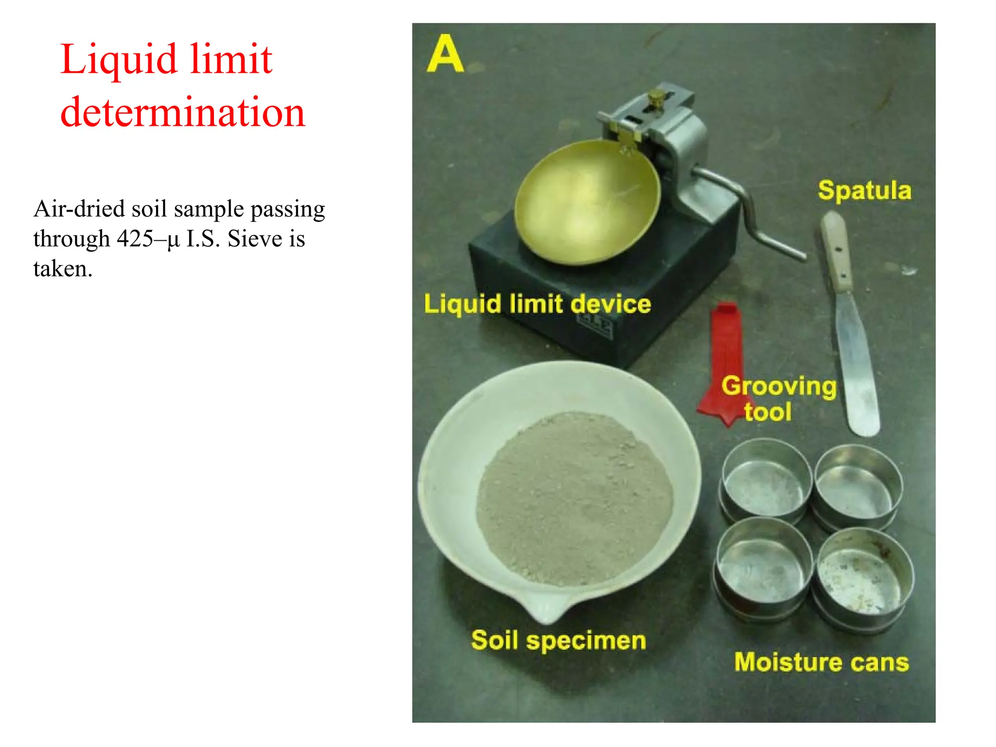
Atterberg Limits
Liquid Limit (wL or LL): min. water content at which soils have
tendency to flow
Clay flows like liquid when w > LL
Plastic Limit (wP or PL):
Lowest water content where the clay is still plastic
Shrinkage Limit (wS or SL):
At w<SL, no volume reduction on drying

Liquid limit
determination
55
Air-dried soil sample passing
through 425–μ I.S. Sieve is
taken.

56
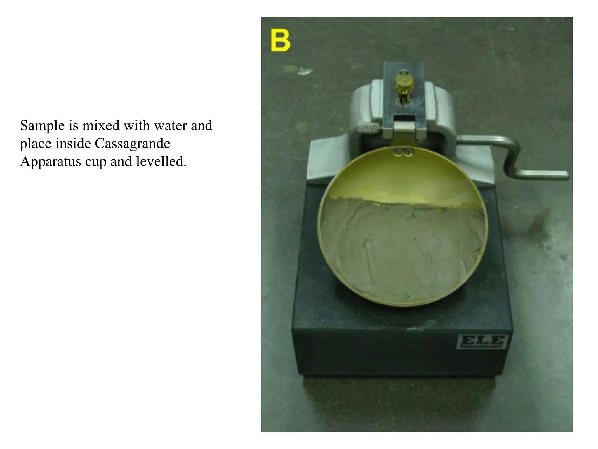
Sample is mixed with water and
place inside Cassagrande
Apparatus cup and levelled.

57
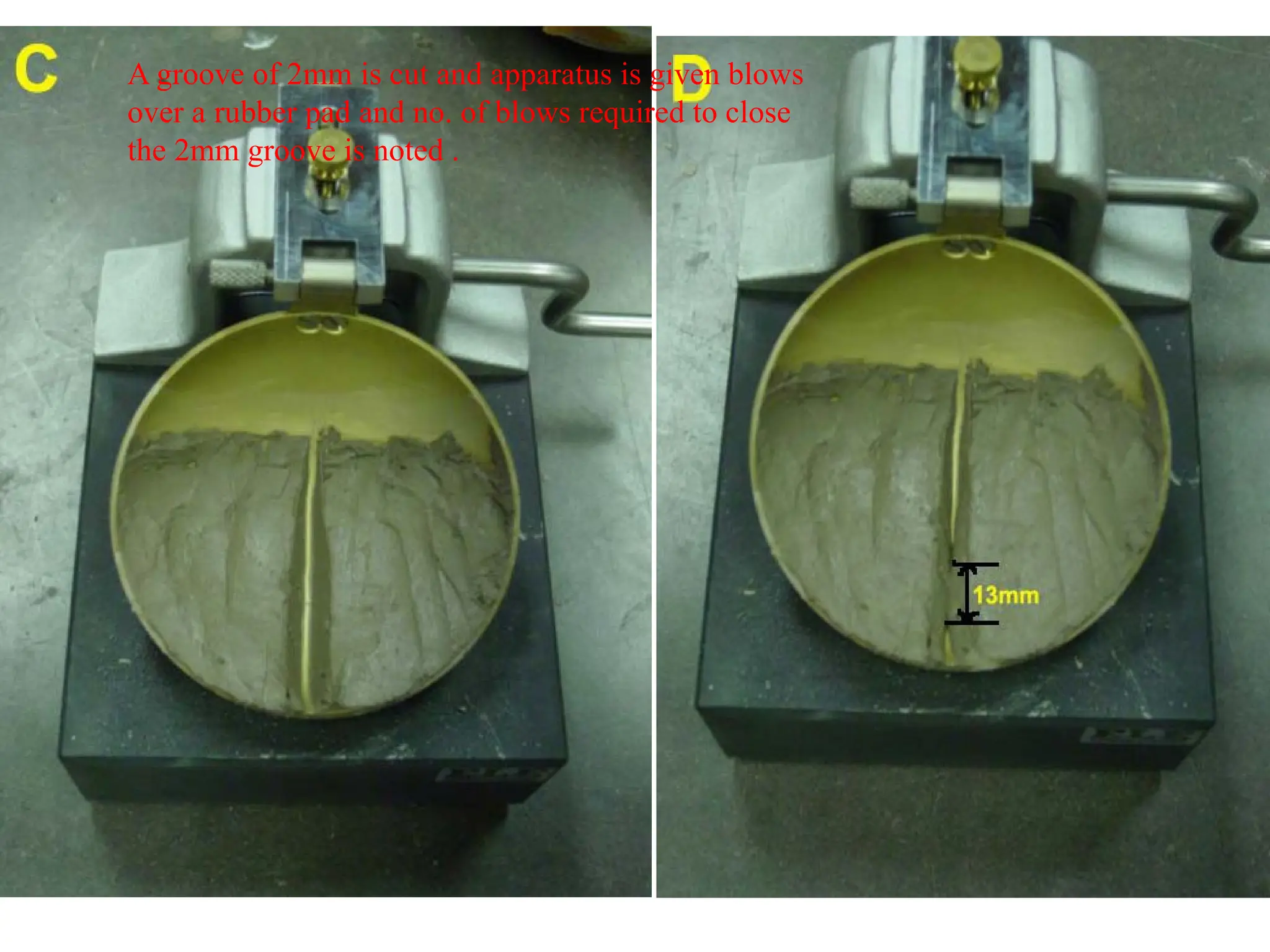
A groove of 2mm is cut and apparatus is given blows
over a rubber pad and no. of blows required to close
the 2mm groove is noted .

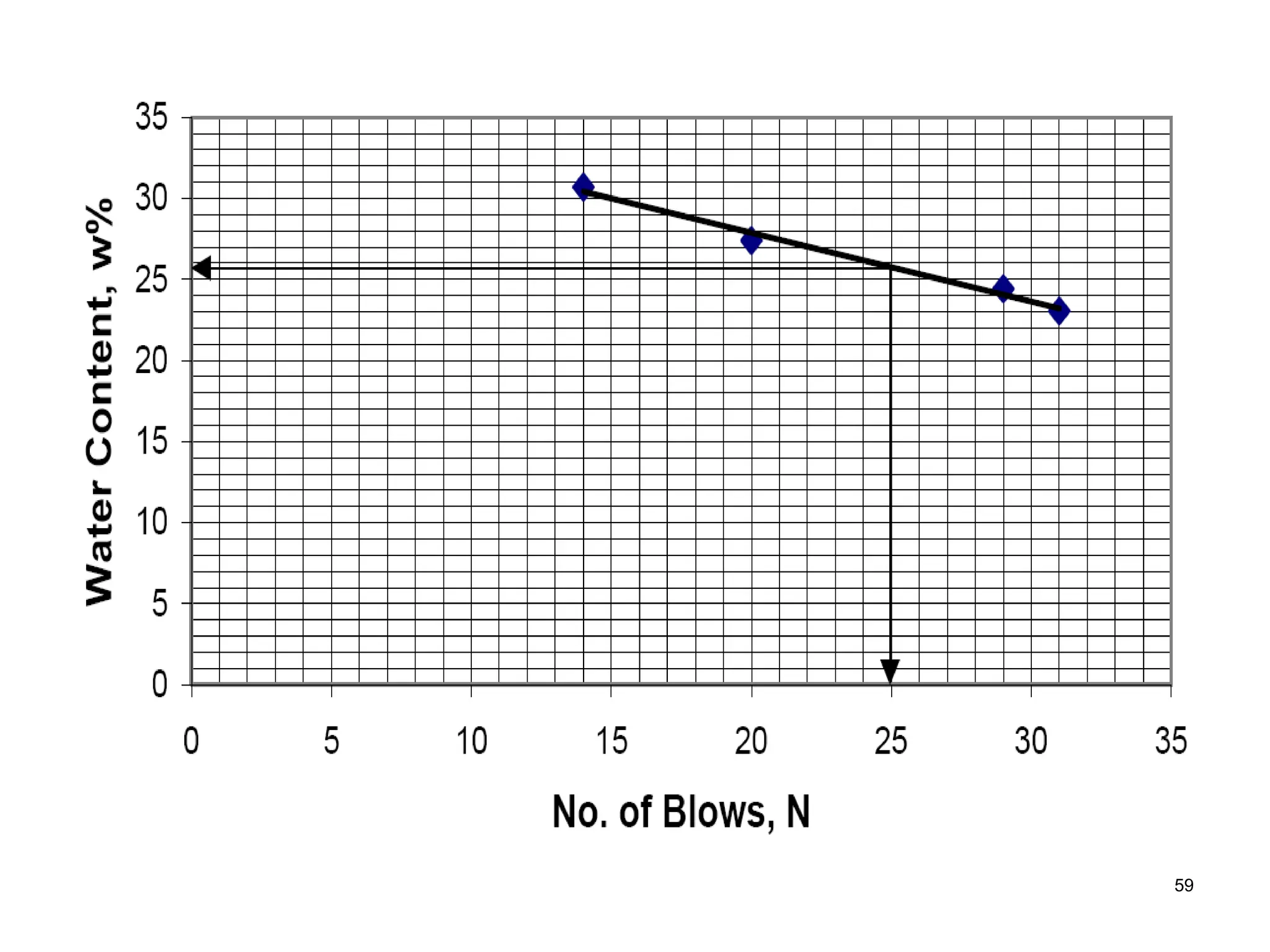
Now same soil is mixed with water content and no. of blows
required to close the 2mm groove is noted as .
Same process is repeated with different water content.
A graph is plotted between %water content and No. of blows
in semi log scale.
The curve is called flow curve and the slope of above curve is
called flow index
Is a soil has a greater flow index, it means that the rate of loss of
shear strength with increase in water content is high.
58

60
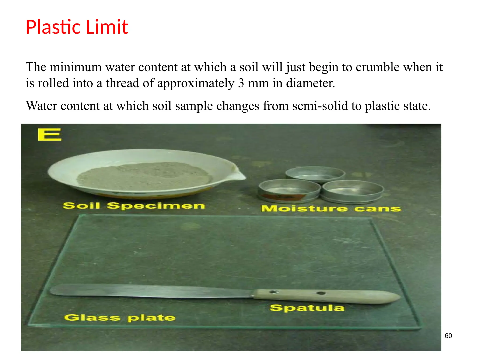
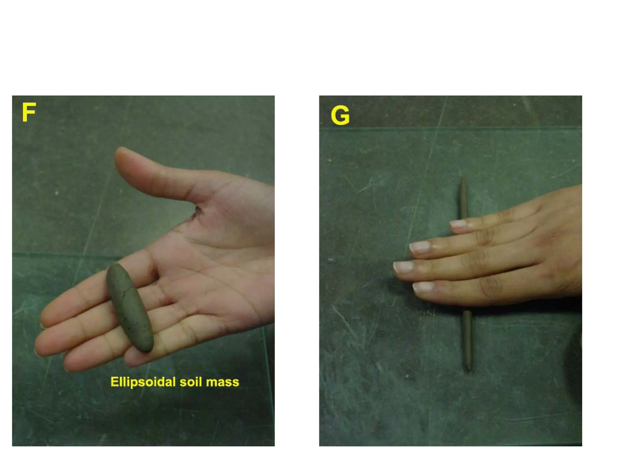
Plastic Limit
The minimum water content at which a soil will just begin to crumble when it
is rolled into a thread of approximately 3 mm in diameter.
Water content at which soil sample changes from semi-solid to plastic state.

62
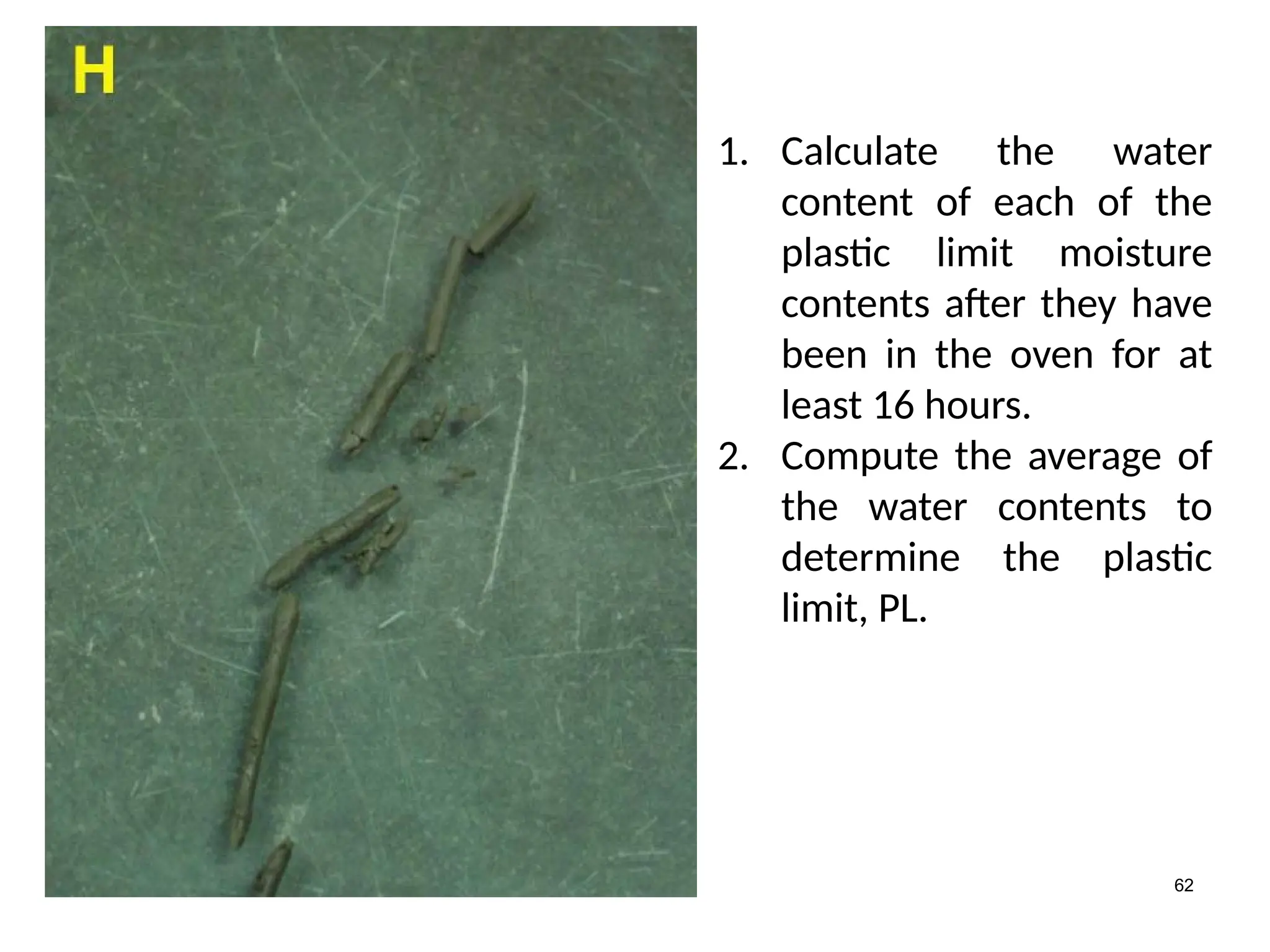
1. Calculate the water
content of each of the
plastic limit moisture
contents after they have
been in the oven for at
least 16 hours.
2. Compute the average of
the water contents to
determine the plastic
limit, PL.

Clays have plastic limit and liquid limit
But LL>>PL
Coarse grained soil like sand and gravel have less liquid limit
and plastic limit generally,
Plastic limit depends upon amount and type of clay mineral in
soil. Hence clay containing fine soils have more plastic limit.
63

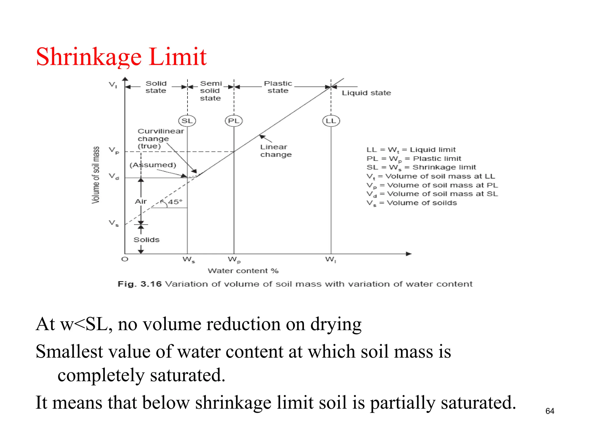
Shrinkage Limit
64
At w<SL, no volume reduction on drying
Smallest value of water content at which soil mass is
completely saturated.
It means that below shrinkage limit soil is partially saturated.

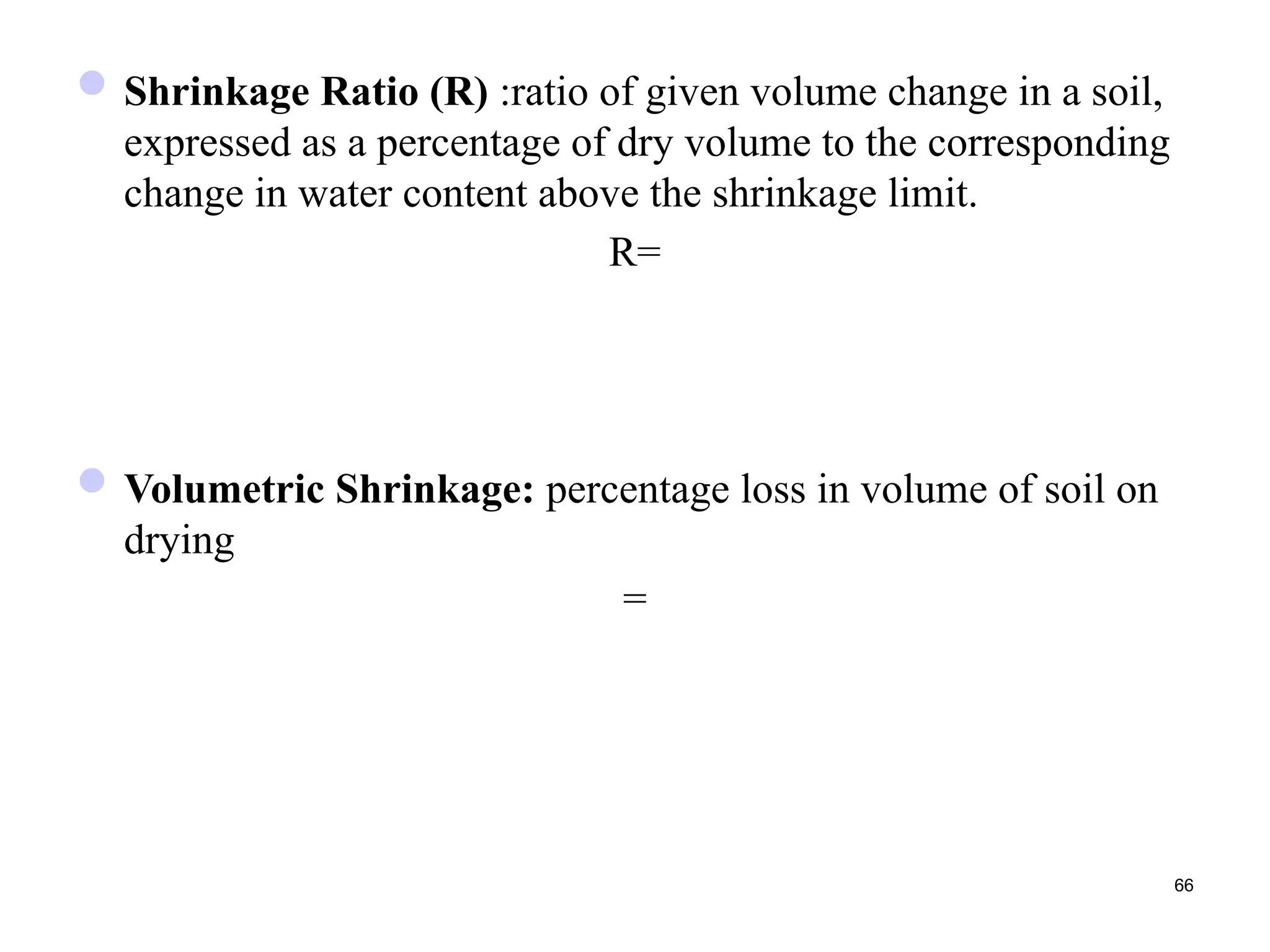
Shrinkage Ratio (R) :ratio of given volume change in a soil,
expressed as a percentage of dry volume to the corresponding
change in water content above the shrinkage limit.
R=
Volumetric Shrinkage: percentage loss in volume of soil on
drying
=
66

Degree of Shrinkage: percentage loss in vol. of soil on drying
corresponding to initial vol.
=
67

68
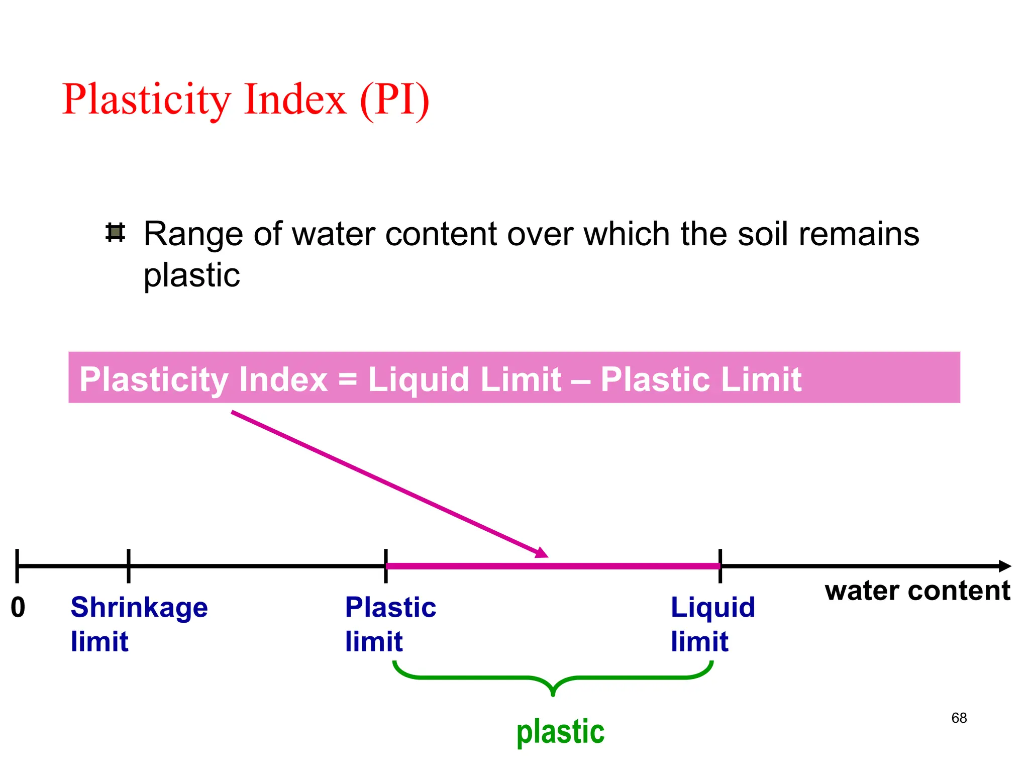
Plasticity Index (PI)
Range of water content over which the soil remains
plastic
Liquid
limit
Shrinkage
limit
Plastic
limit
0
water content
plastic
Plasticity Index = Liquid Limit – Plastic Limit

69
Some Indices
Plasticity Index

70
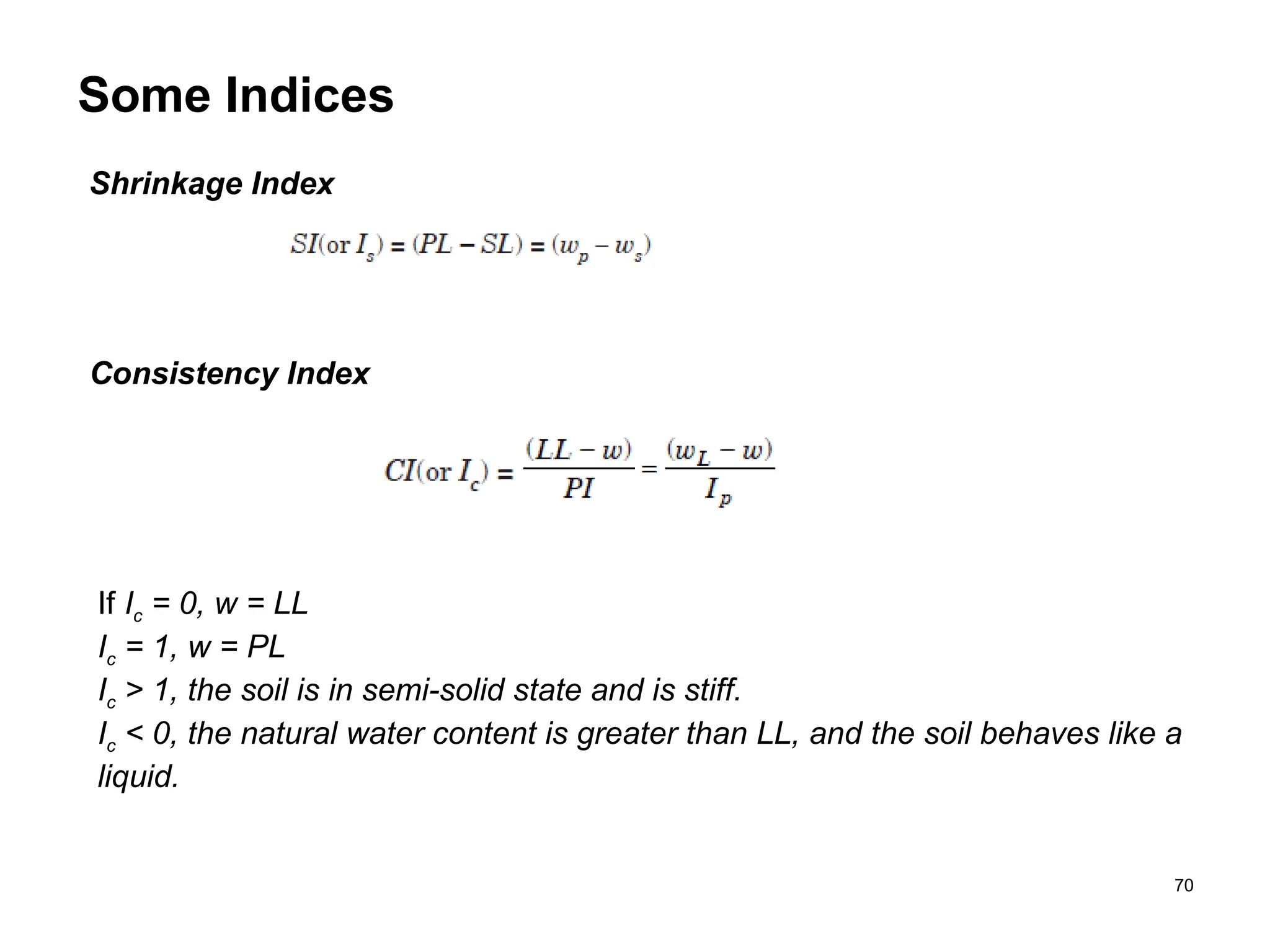
Some Indices
Shrinkage Index
Consistency Index
If Ic = 0, w = LL
Ic = 1, w = PL
Ic > 1, the soil is in semi-solid state and is stiff.
Ic < 0, the natural water content is greater than LL, and the soil behaves like a
liquid.

71
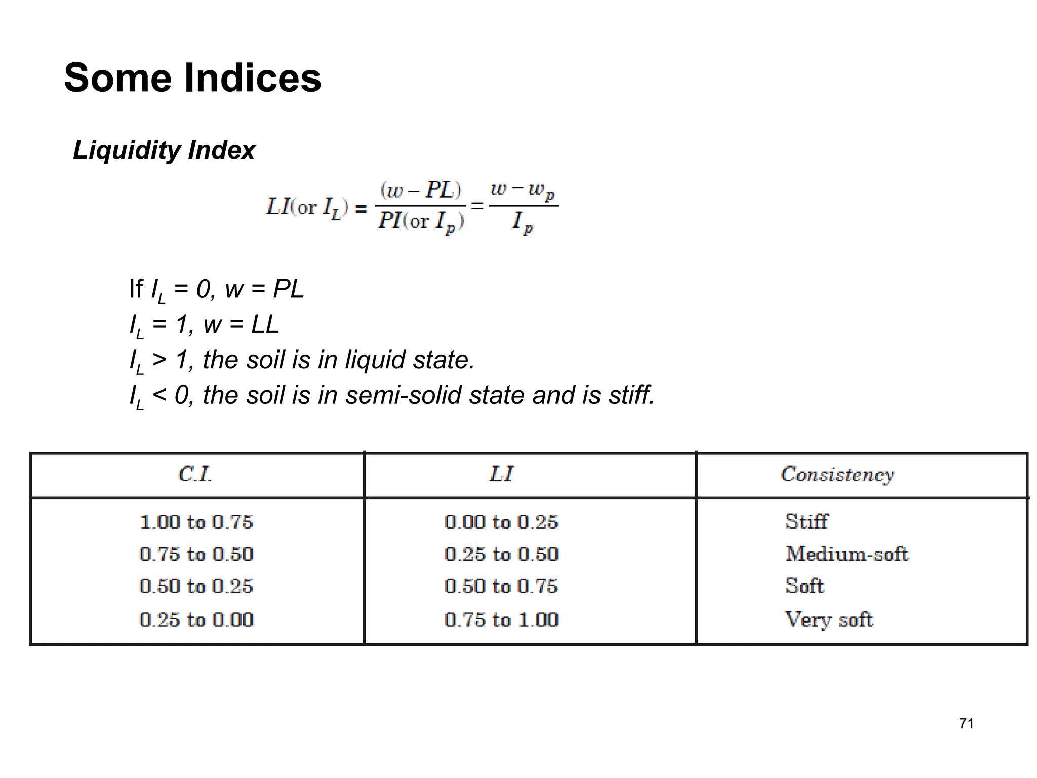
Some Indices
Liquidity Index
If IL = 0, w = PL
IL = 1, w = LL
IL > 1, the soil is in liquid state.
IL < 0, the soil is in semi-solid state and is stiff.

Importance of Atterberg limits
The liquid limit and plasticity index are used to classify fine
soils.
 To understand consistency of soil
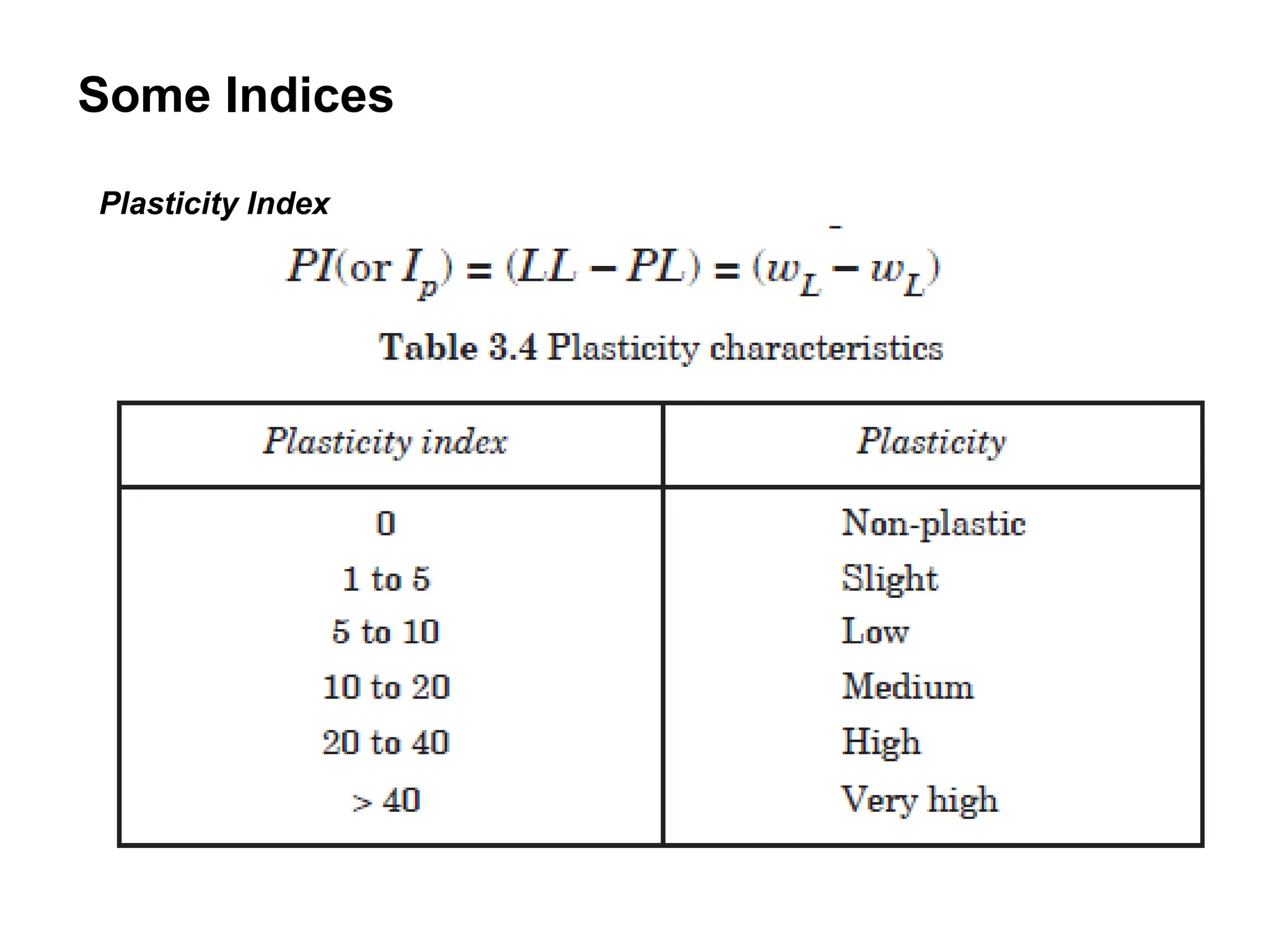
Plasticity index and there meanings
0 - Nonplastic
(1-5)- Slightly Plastic
(5-10) - Low plasticity
(10-20)- Medium plasticity
(20-40)- High plasticity
>40 Very high plasticity
73

The plasticity index is a description of how much a soil
expands and shrinks. When a structure is built on a soil with a
high plasticity index the structures foundation is much more
likely to crack and fail.
The liquid, plastic and shrinkage limit are used for an
approximate evaluation of swelling potential.
The liquid limit can be used for finding an approx value of
compression index Cc
74

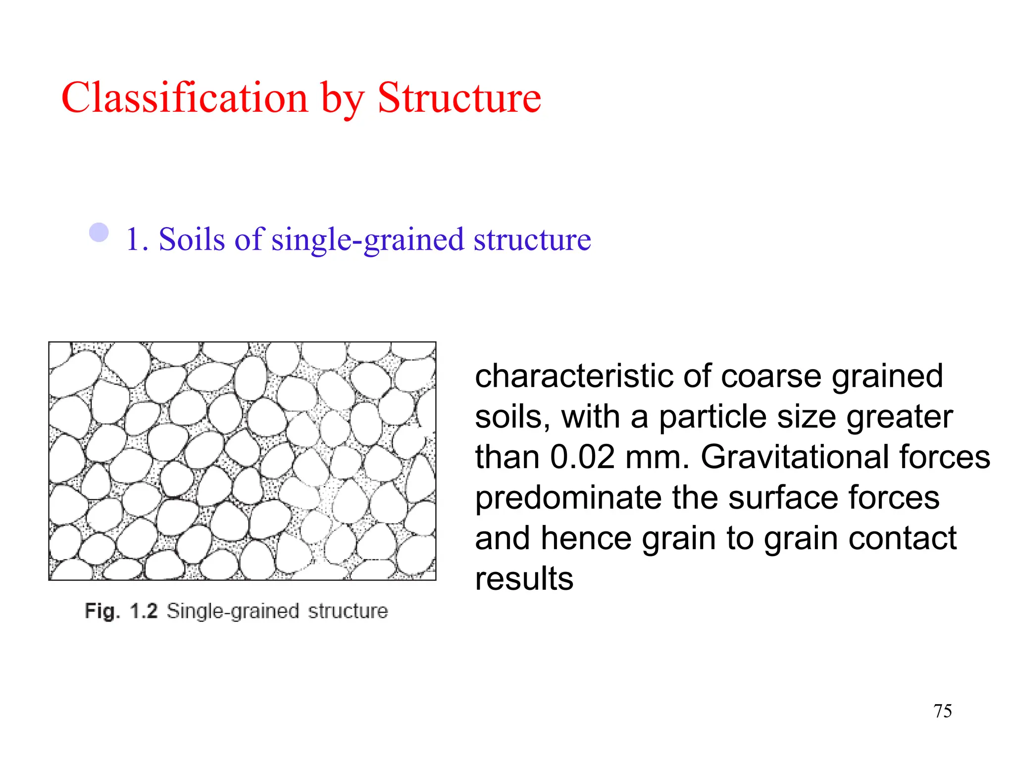
Classification by Structure
1. Soils of single-grained structure
75
characteristic of coarse grained
soils, with a particle size greater
than 0.02 mm. Gravitational forces
predominate the surface forces
and hence grain to grain contact
results

76
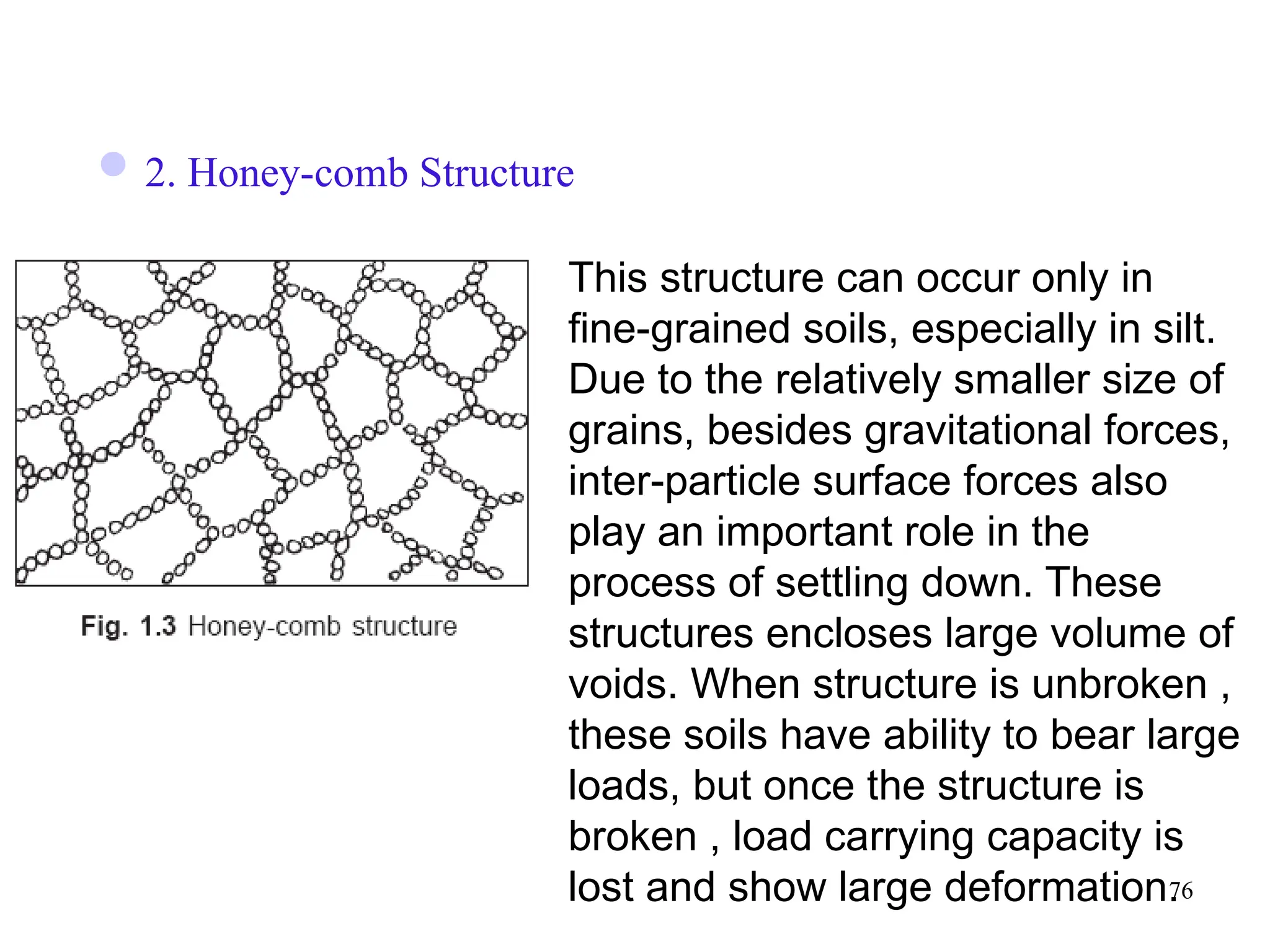
2. Honey-comb Structure
This structure can occur only in
fine-grained soils, especially in silt.
Due to the relatively smaller size of
grains, besides gravitational forces,
inter-particle surface forces also
play an important role in the
process of settling down. These
structures encloses large volume of
voids. When structure is unbroken ,
these soils have ability to bear large
loads, but once the structure is
broken , load carrying capacity is
lost and show large deformation.

77
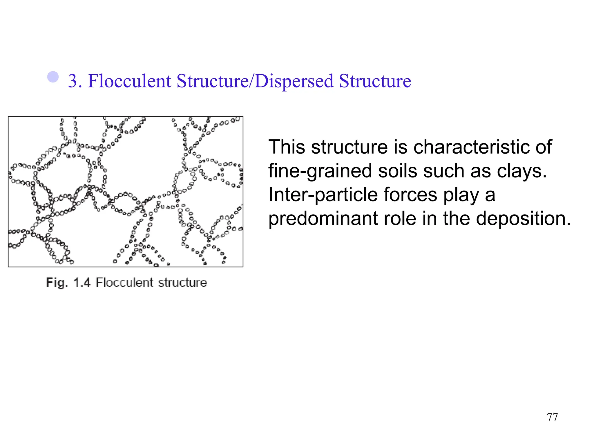
3. Flocculent Structure/Dispersed Structure
This structure is characteristic of
fine-grained soils such as clays.
Inter-particle forces play a
predominant role in the deposition.

79
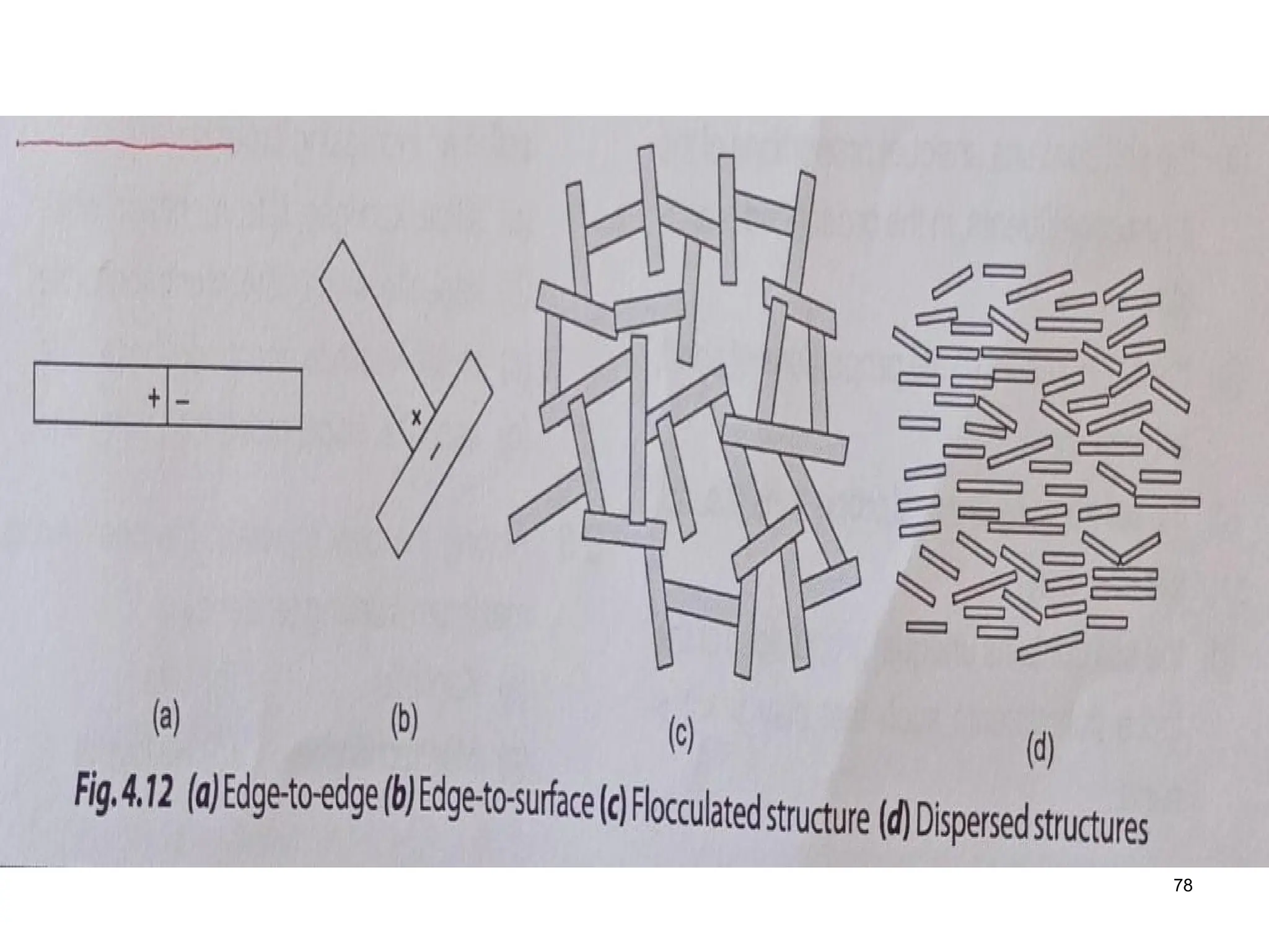
. These soil structures have high volume voids. Particles
joined edge to edge or edge to surface results in a
flocculated structure

80
Dispersed structures develops in clays that have been
remoulded. When flocculated soils are remoulded by nature or
man, converts its edge to edge or edge to surface orientation
into surface to surface orientation.

index properties of soil 2.pptxioohfohof

More Related Content

Similar to index properties of soil 2.pptxioohfohof

Recently uploaded

index properties of soil 2.pptxioohfohof