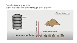
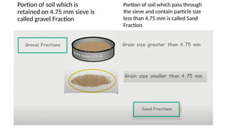
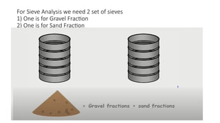
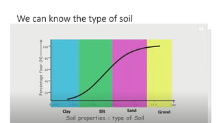
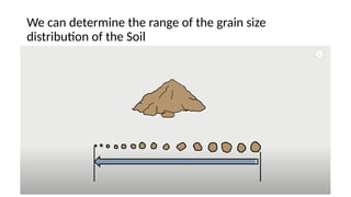
Portion of soilwhich is
retained on 4.75 mm sieve is
called gravel Fraction
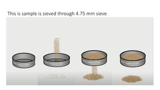
Portion of soil which pass through
the sieve and contain particle size
less than 4.75 mm is called Sand
Fraction
12.
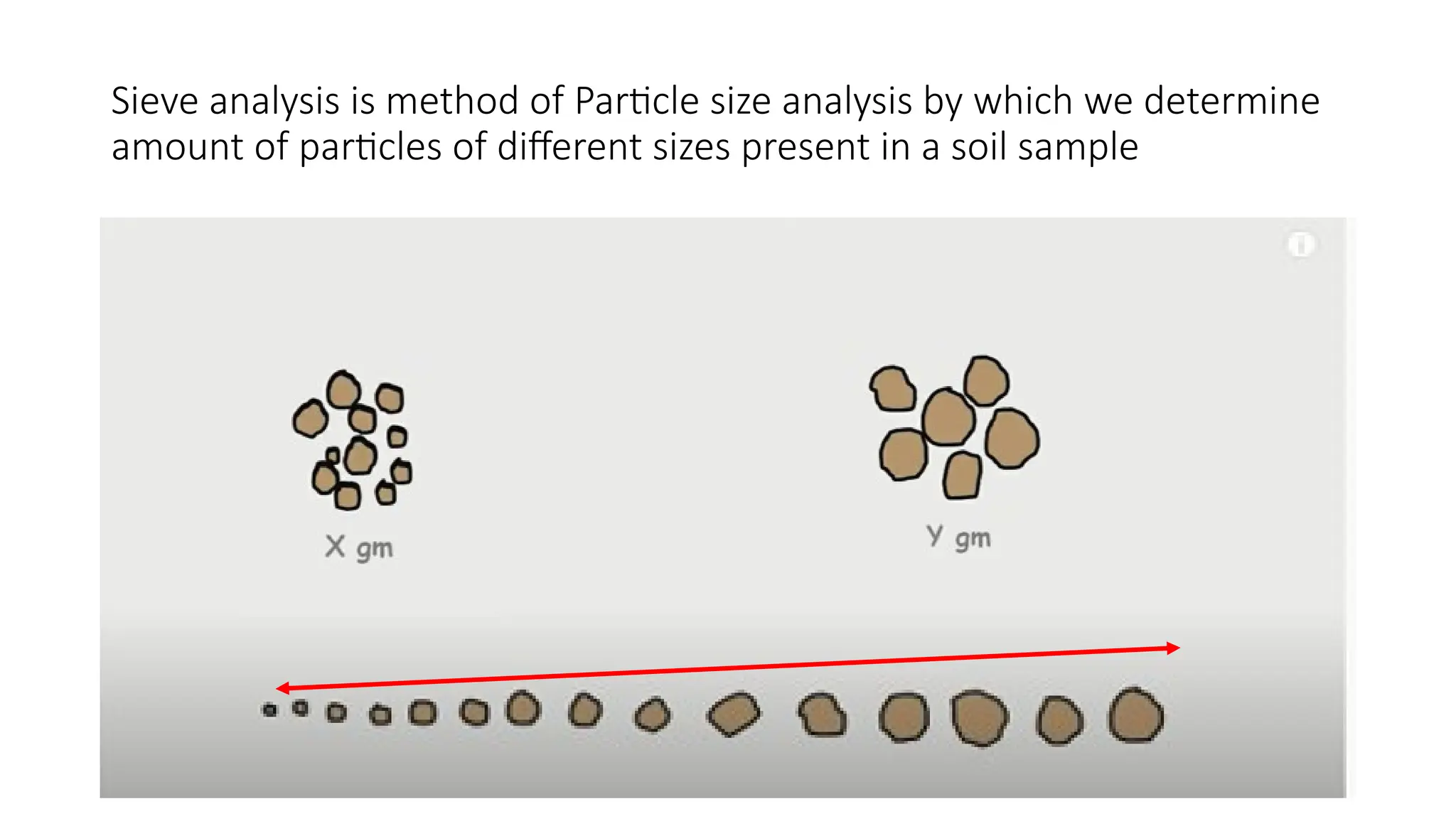
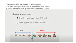
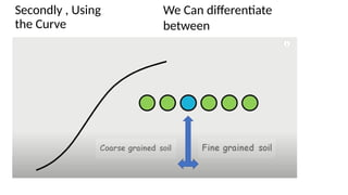
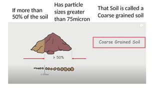
Coarse Grain Soilsare divided into 2 categories
1) Gravels having particle/grain size greater than 4.75 mm
2) Sands having particle/ grain size smaller than 4.75 mm
Gravels
Sand
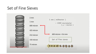
Set of FineSieves
2 mm
1 mm
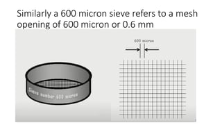
600 micron
425 micron
212 micron
150 micron
75 micron
600 micron = 0.6 mm
17.
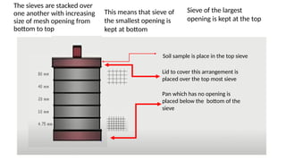
The sieves arestacked over
one another with increasing
size of mesh opening from
bottom to top
This means that sieve of
the smallest opening is
kept at bottom
Sieve of the largest
opening is kept at the top
Pan which has no opening is
placed below the bottom of the
sieve
Soil sample is place in the top sieve
Lid to cover this arrangement is
placed over the top most sieve
18.
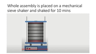
Whole assembly isplaced on a mechanical
sieve shaker and shaked for 10 mins
19.
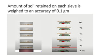
Amount of soilretained on each sieve is
weighed to an accuracy of 0.1 gm
W1
W2
W3
W4
W5
W pan
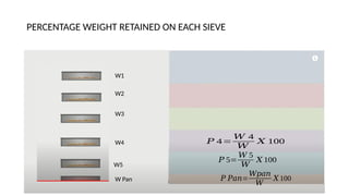
20.
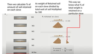
Then we calculate% of
amount of soil retained
on each sieve
W1
W2
W3
W4
W5
W Pan
As weight of Retained soil
on each sieve divided by
total wait of soil Multiplied
by 100
This way we
know what % of
total weight is
retained on a
particular sieve
• .
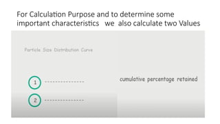
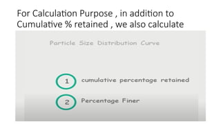
For Calculation Purposeand to determine some
important characteristics we also calculate two Values
23.
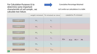
For Calculation Purposes& to
determine some important
characteristic of soil sample , we
calculate two Values
P4
P3 +
P 2+
P1+
Cumulative Percentage Retained
Let’s write our calculations in a table
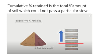
24.
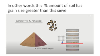
Cumulative % retainedis the total %amount
of soil which could not pass a particular sieve
25.
In other wordsthis % amount of soil has
grain size greater than this sieve
26.
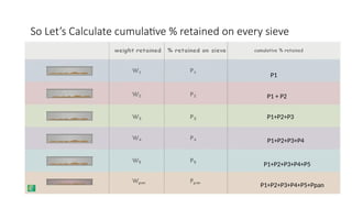
So Let’s Calculatecumulative % retained on every sieve
P1
P1 + P2
P1+P2+P3
P1+P2+P3+P4
P1+P2+P3+P4+P5
P1+P2+P3+P4+P5+Ppan
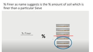
% Finer asname suggests is the % amount of soil which is
finer than a particular Sieve
%
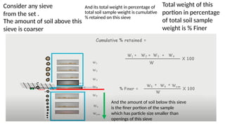
30.
And its totalweight in percentage of
total soil sample weight is cumulative
% retained on this sieve
The amount of soil above this
sieve is coarser
Consider any sieve
from the set .
And the amount of soil below this sieve
is the finer portion of the sample
which has particle size smaller than
openings of this sieve
Total weight of this
portion in percentage
of total soil sample
weight is % Finer
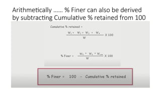
31.
Arithmetically …… %Finer can also be derived
by subtracting Cumulative % retained from 100
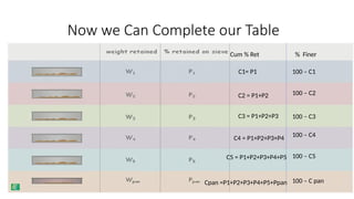
32.
Now we CanComplete our Table
Cum % Ret
C1= P1
C2 = P1+P2
C3 = P1+P2+P3
C4 = P1+P2+P3+P4
C5 = P1+P2+P3+P4+P5
Cpan =P1+P2+P3+P4+P5+Ppan
% Finer
100 – C1
100 – C2
100 – C3
100 – C4
100 – C5
100 – C pan
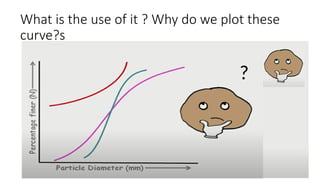
33.
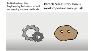
To Understand the
EngineeringBehaviour of soil
we employ various methods
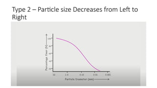
Particle Size Distribution is
most important amongst all
34.
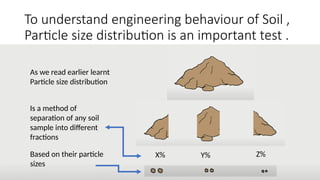
To understand engineeringbehaviour of Soil ,
Particle size distribution is an important test .
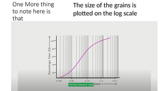
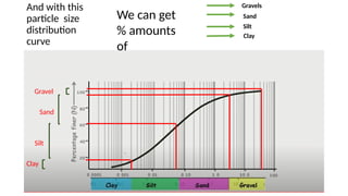
As we read earlier learnt
Particle size distribution
Based on their particle
sizes
Is a method of
separation of any soil
sample into different
fractions
X% Y% Z%
35.
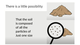
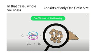
There is alittle possibility
That the soil
is composed
of all the
particles of
Just one size
36.
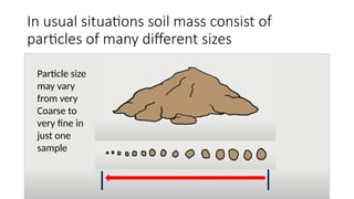
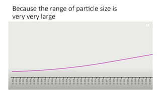
In usual situationssoil mass consist of
particles of many different sizes
Particle size
may vary
from very
Coarse to
very fine in
just one
sample
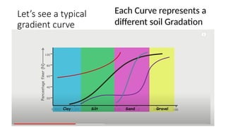
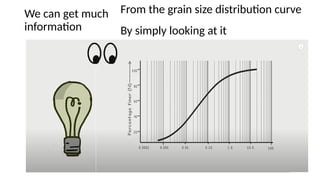
37.
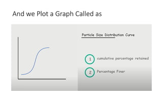
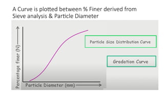
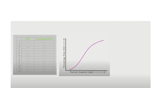
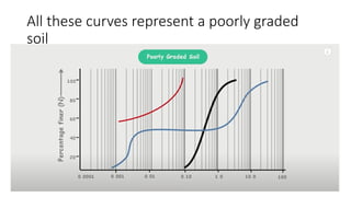
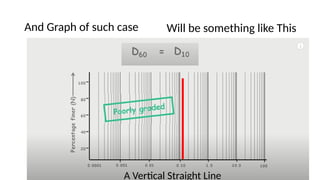
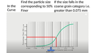
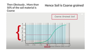
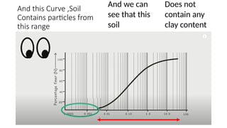
A Curve isplotted between % Finer derived from
Sieve analysis & Particle Diameter
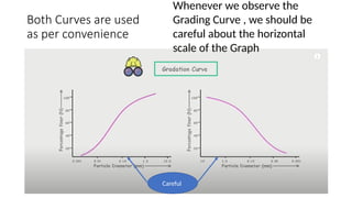
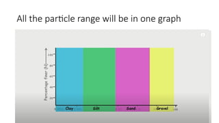
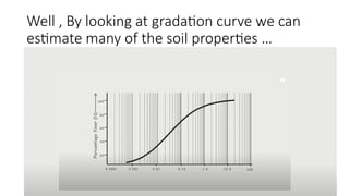
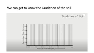
38.
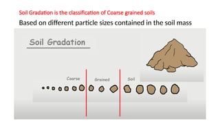
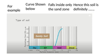
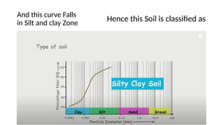
Soil Gradation isthe classification of Coarse grained soils
Based on different particle sizes contained in the soil mass
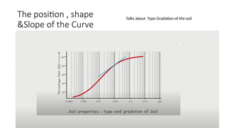
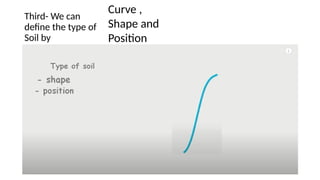
The position ,shape
&Slope of the Curve
Talks about Type Gradation of the soil
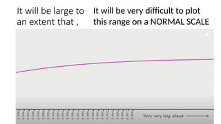
54.
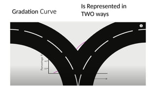
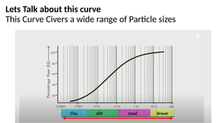
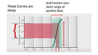
Lets Talk aboutthis curve
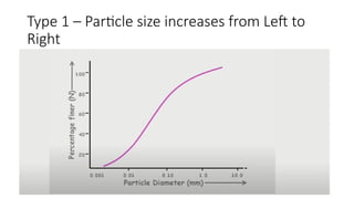
This Curve Civers a wide range of Particle sizes
55.
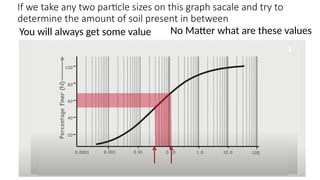
If we takeany two particle sizes on this graph sacale and try to
determine the amount of soil present in between
You will always get some value No Matter what are these values
56.
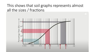
This shows thatsoil graphs represents almost
all the sizes / fractions
57.
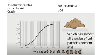
This shows thatthis
particular soil
Graph
Represents a
Soil
Which has almost
all the size of soil
particles present
in it
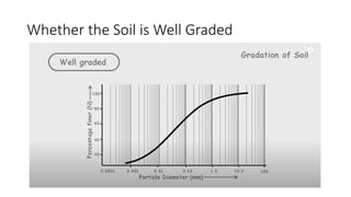
58.
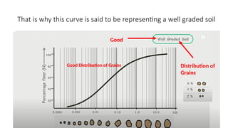
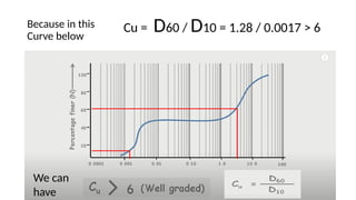
That is whythis curve is said to be representing a well graded soil
Good
Distribution of
Grains
Good Distribution of Grains
59.
Now Lets
take
another
curve
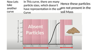
In Thiscurve, there are many
particle sizes, which doesn’t
have representation in the soil
Curve
Absent
Particles
Hence these particles
are not present in the
soil Mass
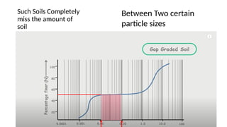
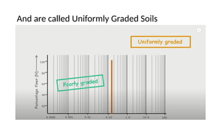
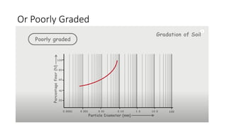
60.
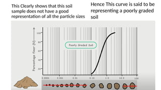
This Clearly showsthat this soil
sample does not have a good
representation of all the particle sizes
Hence This curve is said to be
representing a poorly graded
soil
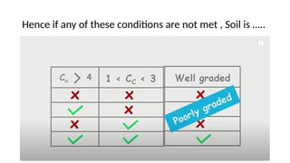
61.
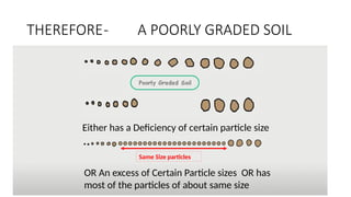
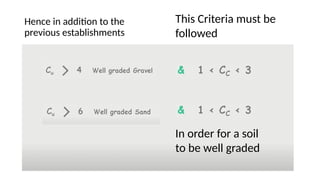
THEREFORE- A POORLYGRADED SOIL
Either has a Deficiency of certain particle size
OR An excess of Certain Particle sizes OR has
most of the particles of about same size
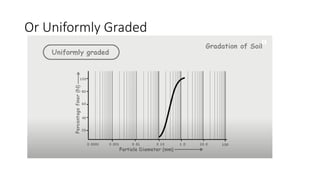
Same Size particles
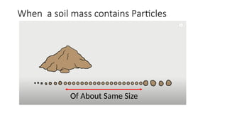
When a soilmass contains Particles
Of About Same Size
64.
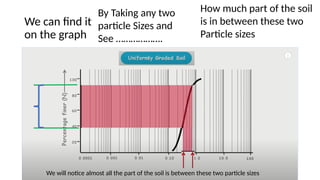
We can findit
on the graph
By Taking any two
particle Sizes and
See ……………….
How much part of the soil
is in between these two
Particle sizes
We will notice almost all the part of the soil is between these two particle sizes
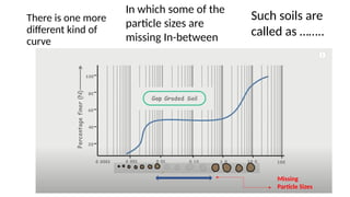
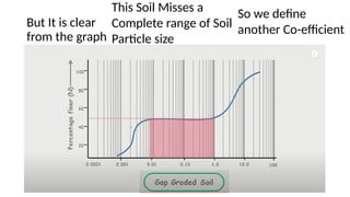
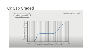
There is onemore
different kind of
curve
In which some of the
particle sizes are
missing In-between
Missing
Particle Sizes
Such soils are
called as ……..
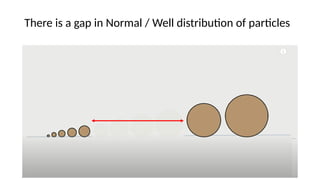
67.
There is agap in Normal / Well distribution of particles
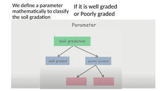
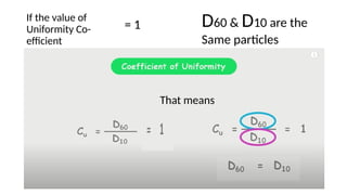
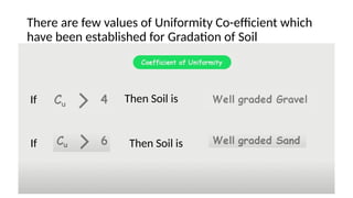
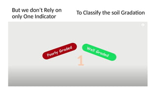
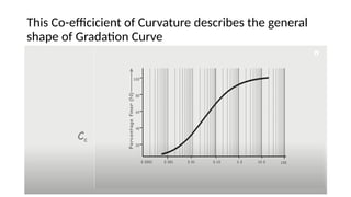
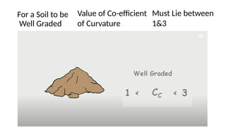
We define aparameter
mathematically to classify
the soil gradation
If it is well graded
or Poorly graded
70.
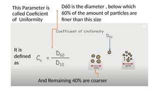
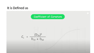
This Parameter is
calledCoeficient
of Uniformity
It is
defined
as
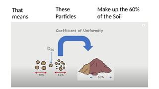
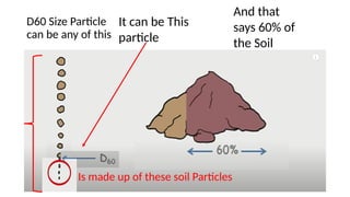
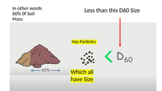
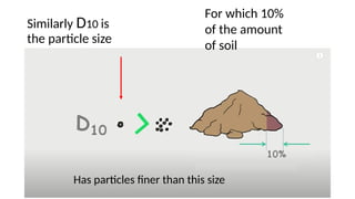
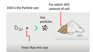
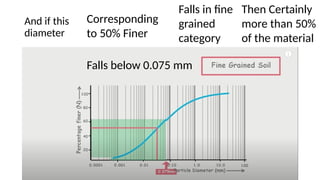
D60 is the diameter , below which
60% of the amount of particles are
finer than this size
And Remaining 40% are coarser


![Geotechnical Engineering-I [Lec #7: Sieve Analysis-2]](https://cdn.slidesharecdn.com/ss_thumbnails/7-180923180808-thumbnail.jpg?width=640&height=640&fit=bounds)


