The document describes implementing the K-Nearest Neighbors (KNN) machine learning algorithm. It discusses taking input data, plotting sample points from the training data, implementing the KNN algorithm to classify test data points based on their distances to training points, and analyzing the results. Code is provided to perform the KNN implementation, including calculating distances, predicting classes, and plotting classified test points.

1. Implementing K-Nearest Neighbors
Dipesh Shome
Department of Computer Science and Engineering,AUST
Ahsanullah University of Science and Technology
Dhaka, Bangladesh
160204045@aust.edu
Abstract—K-Nearest Neighbour is one of the simplest Machine
Learning algorithms based on Supervised Learning technique. K-
NN algorithm assumes the similarity between the new case/data
and available cases and put the new case into the category that
is most similar to the available categories.In this experiment
we implemented the K-NN algorithm which is very simple to
implement. It is robust in noisy data but the computation cost is
high because of calculating distance between the data points for
all the training samples.
Index Terms—K Nearest algorithm, Euclidean distance, K
values,
I. INTRODUCTION
The K-NEAREST NEIGHBOR (KNN) is a supervised
learning based machine learning algorithm. Furthermore it is a
non-parametric method used for classification and regression.
In both cases, the input consists of the k closest training
examples in the feature space. The output depends on whether
K-NN is used for classification or regression. It is also called
a lazy learner algorithm because it does not learn from the
training set immediately instead it stores the dataset and at
the time of classification, it performs an action on the dataset.
II. EXPERIMENTAL DESIGN / METHODOLOGY
A. Description of the different tasks
Task 1: Take input from “train.txt” and plot the points with
different colored markers according to the assigned class label.
Task 2: Implement KNN algorithm. The value of K will be
taken from user. Classify the test points from “test.txt” with
different colored markers according to the predicted class
label.
Task 3: Print the top K distances along with their class
labels and the predicted class to “prediction.txt” for each of
the test data. So, for example, if K = 3, for one of the test
data (3,7), the “prediction.txt” may look like:
Test point: 3, 7
Distance 1: 2 Class: 1
Distance 2: 4 Class: 0
Distance 3: 5 Class: 1
Predicted class: 1
B. Implementation
1) Plotting of all sample data of train data: Here we have
a training dataset which is consist of 14 samples belong to two
different classes. First task is to plot all the data point of both
class.For plotting we import two python library: Numpy and
Matplotlib. Scatter plot function and marker were used to plot
the samples from same classes with same color. Train class 1
is plotted using dot(.) marker with red color and train class
2 is plotted using star(*) marker with blue color.Finally, we
legend the plot and the plotted figure is given in Fig.1.
Fig. 1. Sample point Plotting
2) K-NN implementation and classification of test data and
plotting: In the implementation we calculate the distance of
each test data from all train data. For calculating we use
euclidean distance which is look like :
d(x, y) =
p
(x1 − x2)2 + (y1 − y2)2
After calculating distance we consider the K nearest neighbour
of test data point. K is the user input. Then we use a
counter variable to count the individual number of same class.
Example: If k =3 then we will consider the nearest three train
sample point and count which class is major in number. The
majority class will be consider as the predicted class of test
data points. We predicted the class for all test sample data
points and plot in Fig.2

2. Fig. 2. Test Sample point Plotting
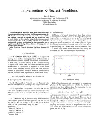
III. RESULT ANALYSIS
When we use k=3 we found 5 points belongs to class 1 and
4 points belongs to class 2. Then again when we use k=5 we
found 5 points belongs to class 2 and 4 points belongs to class
1. If we use higher number of k the variance will be lower
but might be biased.But most the time the optimal value of k
is odd value of
√
n where n is number of sample data.
Fig. 3. Sample point Plotting
IV. CONCLUSION
The purpose of the k Nearest Neighbors (K-NN) algorithm
is to use a database in which the data points are separated into
several separate classes to predict the classification of a new
sample point. This sort of situation is best motivated through
examples. The limitation of this algorithm is it is significantly
slower as the number of examples increases
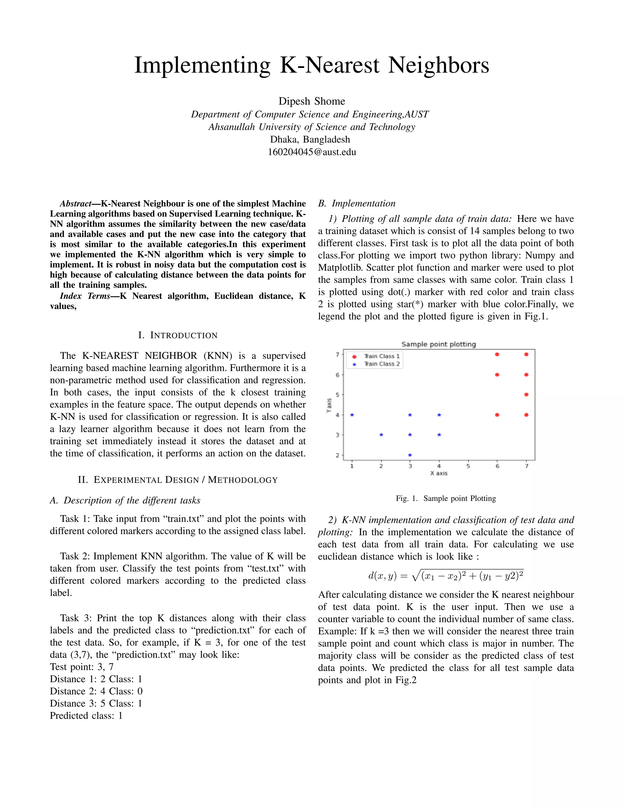
V. ALGORITHM IMPLEMENTATION / CODE
1 import pandas as pd
2 import numpy as np
3 import random
4 import matplotlib.pyplot as plt
5 import math
6
7 p_train = pd.read_csv(’train4.txt’, header=None, sep
=’,’, dtype=’float64’)
8 p_train=np.array(p_train)
9 #print(’Train Dataset:’,p_train)
10
11 p_test = pd.read_csv(’test4.txt’, header=None, sep=’
,’, dtype=’float64’)
12 p_test=np.array(p_test)
13 #print(’Test Dataset:’,p_test)
14
15 shape = p_train.shape
16 row , col = shape[0], shape[1]
17 class_1 = []
18 class_2 = []
19 for i in range(row):
20 if(p_train[i][2] == 1):
21 _list = []
22 _list.append(p_train[i][0])
23 _list.append(p_train[i][1])
24 class_1.append(_list)
25 else:
26 _list = []
27 _list.append(p_train[i][0])
28 _list.append(p_train[i][1])
29 class_2.append(_list)
30
31 w1=np.array(class_1)
32 w2=np.array(class_2)
33
34 fig = plt.figure(figsize=(10,7))
35 ax=plt.subplot()
36 plt.scatter(w1[:,0],w1[:,1],color=’r’,marker=’o’,
alpha=0.8,label=’Train Class 1’)
37 plt.scatter(w2[:,0],w2[:,1],color=’b’,marker=’*’,
alpha=0.8,label=’Train Class 2’)
38 ax.set_ylabel(’Y axis’)
39 ax.set_xlabel(’X axis’)
40 ax.set_title(’Sample point plotting’)
41
42 ax.legend()
43
44
45 k = int(input())
46
47 m = p_train.shape[0]
48 n = p_test.shape[0]
49 classified_testdata = []
50 testing_point=[]
51
52
53 file = open("prediction.txt", "w")
54
55
56
57 for i in range(n):
58 l = []
59 t = []
60 z = []
61 for j in range(m):
62 distance = math.sqrt((p_test[i][0] - p_train
[j][0])**2 + (p_test[i][1] - p_train[j][1])**2)
63 temp = []
64 temp.append(p_train[j][0])
65 temp.append(p_train[j][1])
66 temp.append(p_train[j][2])
67 temp.append(distance)
68 l.append(temp)
69
70
71 l = sorted(l, key=lambda a: a[3])
72 #print(l)
73 count1 = 0
74 count2 = 0

3. 75 for neighbor in range(k):
76 if l[neighbor][2] == 1.0:
77 count1 = count1 + 1
78 elif l[neighbor][2] == 2.0:
79 count2 = count2 + 1
80 if count1>count2:
81 t.append(p_test[i][0])
82 t.append(p_test[i][1])
83 t.append(1)
84 classified_testdata.append(t)
85 else:
86 t.append(p_test[i][0])
87 t.append(p_test[i][1])
88 t.append(2)
89 classified_testdata.append(t)
90
91
92 testing_point=p_test.tolist()
93 print(’Testing point ’,testing_point[i])
94 file.write(’Testing point ’ + repr(testing_point
[i]) + ’n’)
95 for r in range(k):
96 print(’Distance ’,r+1 ,’:’,l[r][3],’class’,l
[r][2])
97 file.write(’Distance ’+ repr(r+1) + ’:’ +
repr(l[r][3]) + ’ ’ + ’class’+ repr(l[r][2]) +
’n’)
98 print(’Predicted_class ’ + repr(
classified_testdata[i][2]) + ’n’)
99 file.write(’Predicted_class: ’ + repr(
classified_testdata[i][2]) + ’nn’)
100
101 file.close()
102
103
104
105 classified_testdata
106 p_classified=np.array(classified_testdata)
107 #print(’Classified data:’,p_classified)
108
109
110 shape = p_classified.shape
111 row , col = shape[0], shape[1]
112 class_1 = []
113 class_2 = []
114 for i in range(row):
115 if(p_classified[i][2] == 1):
116 _list = []
117 _list.append(p_classified[i][0])
118 _list.append(p_classified[i][1])
119 class_1.append(_list)
120 else:
121 _list = []
122 _list.append(p_classified[i][0])
123 _list.append(p_classified[i][1])
124 class_2.append(_list)
125
126 w1=np.array(class_1)
127 w2=np.array(class_2)
128 ax=plt.subplot()
129 plt.scatter(w1[:,0],w1[:,1],color=’g’,marker=’+’,
alpha=0.8,label=’Test Class 1’)
130 plt.scatter(w2[:,0],w2[:,1],color=’k’,marker=’s’,
alpha=0.8,label=’Test Class 2’)
131 ax.set_ylabel(’Y axis’)
132 ax.set_xlabel(’X axis’)
133 ax.set_title(’Sample points plotting’)
134
135 ax.legend()
136 plt.show()
REFERENCES
[1] K Nearest Neighbor: K Nearest Neighbor Algorithm
[2] G. Eason, B. Noble, and I. N. Sneddon, “On certain integrals of
Lipschitz-Hankel type involving products of Bessel functions,” Phil.
Trans. Roy. Soc. London, vol. A247, pp. 529–551, April 1955.