Downloaded 14 times


![33
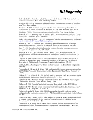
Categorical Principal Components Analysis (CATPCA)
Supplementary Objects. Specify the case number of the object, or the first and last case numbers
of a range of objects, that you want to make supplementary and then click Add. Continue until
you have specified all of your supplementary objects. If an object is specified as supplementary,
then case weights are ignored for that object.
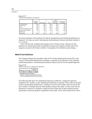
Normalization Method. You can specify one of five options for normalizing the object scores and
the variables. Only one normalization method can be used in a given analysis.
Variable Principal. This option optimizes the association between variables. The coordinates
of the variables in the object space are the component loadings (correlations with principal
components, such as dimensions and object scores). This is useful when you are primarily
interested in the correlation between the variables.
Object Principal. This option optimizes distances between objects. This is useful when you are
primarily interested in differences or similarities between the objects.
Symmetrical. Use this normalization option if you are primarily interested in the relation
between objects and variables.
Independent. Use this normalization option if you want to examine distances between objects
and correlations between variables separately.
Custom. You can specify any real value in the closed interval [–1, 1]. A value of 1 is equal to
the Object Principal method, a value of 0 is equal to the Symmetrical method, and a value of
–1 is equal to the Variable Principal method. By specifying a value greater than –1 and less
than 1, you can spread the eigenvalue over both objects and variables. This method is useful
for making a tailor-made biplot or triplot.
Criteria. You can specify the maximum number of iterations the procedure can go through in its
computations. You can also select a convergence criterion value. The algorithm stops iterating if
the difference in total fit between the last two iterations is less than the convergence value or if
the maximum number of iterations is reached.
Label Plots By. Allows you to specify whether variables and value labels or variable names and
values will be used in the plots. You can also specify a maximum length for labels.
Plot Dimensions. Allows you to control the dimensions displayed in the output.
Display all dimensions in the solution. All dimensions in the solution are displayed in a
scatterplot matrix.
Restrict the number of dimensions. The displayed dimensions are restricted to plotted pairs. If
you restrict the dimensions, you must select the lowest and highest dimensions to be plotted.
The lowest dimension can range from 1 to the number of dimensions in the solution minus 1
and is plotted against higher dimensions. The highest dimension value can range from 2 to the
number of dimensions in the solution and indicates the highest dimension to be used in plotting
the dimension pairs. This specification applies to all requested multidimensional plots.
Configuration. You can read data from a file containing the coordinates of a configuration. The
first variable in the file should contain the coordinates for the first dimension, the second variable
should contain the coordinates for the second dimension, and so on.](https://image.slidesharecdn.com/ibmspsscategories-140731223507-phpapp02/85/Ibm-spss-categories-47-320.jpg)


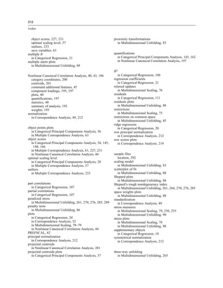
![61
Multiple Correspondence Analysis
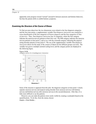
Independent. Use this normalization option if you want to examine distances between objects
and correlations between variables separately.
Custom. You can specify any real value in the closed interval [–1, 1]. A value of 1 is equal to
the Object Principal method, a value of 0 is equal to the Symmetrical method, and a value of
–1 is equal to the Variable Principal method. By specifying a value greater than –1 and less
than 1, you can spread the eigenvalue over both objects and variables. This method is useful
for making a tailor-made biplot or triplot.
Criteria. You can specify the maximum number of iterations the procedure can go through in its
computations. You can also select a convergence criterion value. The algorithm stops iterating if
the difference in total fit between the last two iterations is less than the convergence value or if
the maximum number of iterations is reached.
Label Plots By. Allows you to specify whether variables and value labels or variable names and
values will be used in the plots. You can also specify a maximum length for labels.
Plot Dimensions. Allows you to control the dimensions displayed in the output.
Display all dimensions in the solution. All dimensions in the solution are displayed in a
scatterplot matrix.
Restrict the number of dimensions. The displayed dimensions are restricted to plotted pairs. If
you restrict the dimensions, you must select the lowest and highest dimensions to be plotted.
The lowest dimension can range from 1 to the number of dimensions in the solution minus 1
and is plotted against higher dimensions. The highest dimension value can range from 2 to the
number of dimensions in the solution and indicates the highest dimension to be used in plotting
the dimension pairs. This specification applies to all requested multidimensional plots.
Configuration. You can read data from a file containing the coordinates of a configuration. The
first variable in the file should contain the coordinates for the first dimension, the second variable
should contain the coordinates for the second dimension, and so on.
Initial. The configuration in the file specified will be used as the starting point of the analysis.
Fixed. The configuration in the file specified will be used to fit in the variables. The variables
that are fitted in must be selected as analysis variables, but, because the configuration is
fixed, they are treated as supplementary variables (so they do not need to be selected as
supplementary variables).
Multiple Correspondence Analysis Output
The Output dialog box allows you to produce tables for object scores, discrimination measures,
iteration history, correlations of original and transformed variables, category quantifications for
selected variables, and descriptive statistics for selected variables.](https://image.slidesharecdn.com/ibmspsscategories-140731223507-phpapp02/85/Ibm-spss-categories-75-320.jpg)


![134
Chapter 9
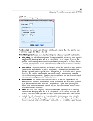
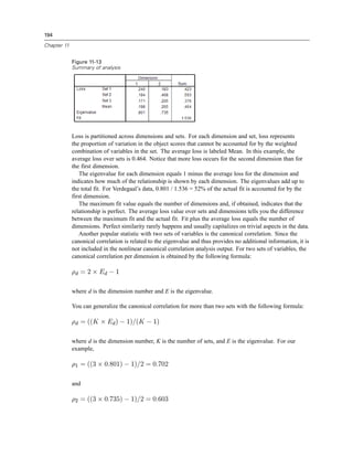
Figure 9-56
Chart Builder
To see a scatterplot of the transformed variables, recall the Chart Builder, and click Reset to
clear your previous selections.
E Select the Scatter/Dot gallery and choose Simple Scatter.
E Select Daily ozone level Quantification [TRA1_3] as the y-axis variable and Day of the year
Quantification [TRA2_3] as the x-axis variable.
E Click OK.](https://image.slidesharecdn.com/ibmspsscategories-140731223507-phpapp02/85/Ibm-spss-categories-148-320.jpg)


This document provides an overview and user guide for IBM SPSS Categories 20, which provides optimal scaling procedures for analyzing categorical data. It introduces key concepts of optimal scaling and discusses the appropriate uses of six procedures: categorical regression, categorical principal components analysis, nonlinear canonical correlation analysis, correspondence analysis, multiple correspondence analysis, and multidimensional scaling. The document also provides details on executing each procedure and interpreting their outputs.